The eWaterCycle platform for open and FAIR hydrological collaboration

Hutton et al. (2016) argued that computational hydrology can only be a proper science if the hydrological community makes sure that hydrological model studies are executed and presented in a reproducible manner. Hut, Drost and van de Giesen replied that to achieve this hydrologists should not “re-invent the water wheel” but rather use existing technology from other fields (such as containers and ESMValTool) and open interfaces (such as the Basic Model Interface, BMI) to do their computational science (Hut et al., 2017). With this paper and the associated release of the eWaterCycle platform and software package (available on Zenodo: https://doi.org/10.5281/zenodo.5119389, Verhoeven et al., 2022), we are putting our money where our mouth is and providing the hydrological community with a “FAIR by design” (FAIR meaning findable, accessible, interoperable, and reproducible) platform to do science.

The eWaterCycle platform separates the experiments done on the model from the model code. In eWaterCycle, hydrological models are accessed through a common interface (BMI) in Python and run inside of software containers. In this way all models are accessed in a similar manner facilitating easy switching of models, model comparison and model coupling. Currently the following models and model suites are available through eWaterCycle: PCR-GLOBWB 2.0, wflow, Hype, LISFLOOD, MARRMoT, and WALRUS While these models are written in different programming languages they can all be run and interacted with from the Jupyter notebook environment within eWaterCycle. Furthermore, the pre-processing of input data for these models has been streamlined by making use of ESMValTool. Forcing for the models available in eWaterCycle from well-known datasets such as ERA5 can be generated with a single line of code. To illustrate the type of research that eWaterCycle facilitates, this paper includes five case studies: from a simple “hello world” where only a hydrograph is generated to a complex coupling of models in different languages.

In this paper we stipulate the design choices made in building eWaterCycle and provide all the technical details to understand and work with the platform. For system administrators who want to install eWaterCycle on their infrastructure we offer a separate installation guide. For computational hydrologists that want to work with eWaterCycle we also provide a video explaining the platform from a user point of view (https://youtu.be/eE75dtIJ1lk, last access: 28 June 2022)​​​​​​​.

With the eWaterCycle platform we are providing the hydrological community with a platform to conduct their research that is fully compatible with the principles of both Open Science and FAIR science.

1 Introduction

In hydrology, scientists try to better quantify the movement of water in, out of, and through the land surface and rivers in order to better predict droughts, floods, navigation hazards, and reservoir operations (Wood et al., 2011). In addition, better understanding of hydrological processes will allow determination of anthropogenic and climate change impacts on the hydrological cycle (McMillan et al., 2020).

From a hydrological point of view, every field, every street, and every part of the world is different. We may have adequate descriptions of how water moves through plants and soils at small scales, but the medium is never the same from one spot to the next. This is the curse of locality (Bierkens, 2015). Nonlinear processes need to be integrated over time and space in the presence of tremendous natural and human-made heterogeneity.

Traditionally, the hydrological community has dealt with this curse by building custom models for small natural watersheds (Beven, 2001). Hydrologists often work with “effective parameters” (Kirchner, 2006; Bárdossy and Singh, 2008), parameters that cannot be measured directly but describe aggregated movement of water through the environment. Typical models are partially based on first-principle physics (mass, momentum, and energy balances) and partially on (statistical or heuristic) assumptions that simplify the complex reality.

Local process knowledge is used to conceptualize many local models by hydrologists from all over the world. This leads to a plethora of local models exhibiting great diversity in the exact methodologies applied, competing hypotheses of hydrologic behavior, technology stacks and programming languages used in these models (Hutton et al., 2016; Hut et al., 2017). Although a wealth of knowledge is encoded in these models, this knowledge is hardly shared due to the technical difficulties of working with models created by other researchers. As a result, models are often chosen based on availability and familiarity, rather than suitability for the research performed (Addor and Melsen, 2019), severely hindering scientific progress in the hydrological community.

Fortunately, the problem of lack of sharing scientific results has recently been picked up as an important topic by the wider academic community. Open Science, where data, publications and software are shared publicly, is deemed more and more important both by researchers and funders (Hall et al., 2022). In addition, the FAIR principles (Wilkinson et al., 2016) describe that all data resulting from research must be made Findable, Accessible, Interoperable, and Reproducible (FAIR). Recently, FAIR has also been extended to software (https://fair-software.eu/, last access: 28 June 2022​​​​​​​) and other academic output.

To enable significant progress in the sharing of hydrological knowledge, we introduce the concept of FAIR hydrological models. FAIR hydrological models make it possible for other researchers to use a model to generate novel scientific results without needing extensive support from the original authors. Any preexisting hydrological model can be made FAIR by adding open interfaces and documentation. With a model that has been made FAIR, it is not only possible to re-create the experiments done by the authors of that model but also to perform novel research by applying the model to different locations with different settings or input data. For a model to be FAIR, not only do the software and required data need to be available but models need to be properly documented and have well-defined interfaces. FAIR Hydrological models have a lower barrier of entry and create scientific results that are as open and FAIR as possible, thereby truly enabling researchers to build on each others results.

In this paper we introduce the eWaterCycle platform, a platform where hydrologists can work with each other or add their own FAIR models. To the best of our knowledge, eWaterCycle is the first platform for hydrological modeling that focuses on providing access to pre-existing models and data sources in a way in which the platform handles the computer and data science aspects to allow the hydrologists to focus on the hydrology. The goal of the eWaterCycle platform is to be a trailblazer for making hydrological modeling open and FAIR. The eWaterCycle platform is designed to support researchers, including graduate students (MSc and PhD levels), to run hydrological experiments with ease, focusing on the science rather than the technology. The platform is designed to enable users to run a simple experiment, such as generating a hydrograph for a certain catchment with a certain model within minutes of getting started, while also giving users the freedom to perform very advanced experiments, such as multi-model coupling and interfering in model states during runtime. With this, we aim to reduce the cycle time in going from idea to experiment (from months to days) and to support fully reproducible experiments. We embrace what has been done already by not rewriting all models from scratch but sharing, reusing, coupling, and building on existing models. The methods and technology developed within the eWaterCycle platform are reusable both inside and outside of Hydrology.

To illustrate how to use the eWaterCycle platform as a hydrologist and demonstrate the type of experiments one can do on the platform (coupling, calibrating, comparing scenarios, etc.), a series of Jupyter notebooks is provided with this paper that showcase the platform. For scientists who want to work with the platform as users, a separate video where a hands-on demonstration of the models is given is available on YouTube (https://youtu.be/eE75dtIJ1lk, last access: 28 June 2022​​​​​​​), and for archiving purposes it is also available on Zenodo (Hut, 2021). The remainder of this paper covers the rationale and the technology behind the platform.

In the eWaterCycle project, we strongly believe that the best approach for generating impact is to build on existing efforts as much as possible. We make use of container technology (specifically Docker (https://www.docker.com, last access: 28 June 2022​​​​​​​) and Singularity (https://sylabs.io/singularity/, last access: 28 June 2022​​​​​​​) that allows capture and preservation of software environments. Pre-processing of forcing data is done using the ESMValTool (Righi et al., 2020), originally developed in the climate sciences. We use Jupyter (https://jupyter.org, last access: 28 June 2022​​​​​​​) as the main user interface to our system. The Basic Model Interface (BMI) (Hutton et al., 2020) provides a stable, easy to implement interface to an existing model. For sharing software, data and results in a FAIR manner, we rely on GitHub (https://github.com, last access: 28 June 2022, HydroShare (Horsburgh et al., 2015)) and Zenodo (https://zenodo.org, last access: 28 June 2022​​​​​​​). Any software contributions that we create in the eWaterCycle project are purposely small and independent, and thus there is a high chance that our components are reusable by other projects in turn.

The eWaterCycle platform can incorporate any existing model with ease, be it conceptual, semi-distributed or distributed, in any commonly used programming language. An alternative and often-used approach to making hydrological models FAIR is to create a single model framework that incorporates as many model concepts as possible. This usually requires significant modifications to a model code, and sometimes even a complete rewrite, to fit within the model framework. The result is a coherent set of models that can be interchanged relatively easily. Examples of such model frameworks include wflow (Schellekens et al., 2020), SUMMA (Clark et al., 2015), MARRMoT (Knoben et al., 2019), and Raven (Craig et al., 2020). In a way this approach can be seen as orthogonal to the eWaterCycle platform, as both approaches can be combined. In the eWaterCycle platform, we have incorporated the wflow and MARRMoT frameworks, making it possible to use any of the models within these frameworks within eWaterCycle. Incorporating the SUMMA framework is on the long-term list of goals for the eWaterCycle platform as well but has not been finished at the time of writing.

There are several other platforms that support open and FAIR hydrology that eWaterCycle connects to. Hydroshare (Horsburgh et al., 2015) focuses on making hydrological data FAIR. It offers a service to publish and access datasets in a Jupyter notebook environment. Unlike eWaterCycle, Hydroshare offers no support when using datasets for an experiment and simply provides data as is. Hydroshare can be used to store data resulting from eWaterCycle experiments in a FAIR manner.

A more structured way of acquiring data for use in a hydrological model is used in HydroDS (Gichamo et al., 2020). HydroDS provides a web service where users can call upon the service to download data in a format suitable for their model. HydroShare and HydroDS can also be combined to generate and store data needed to run models (Gan et al., 2020).

The Community Surface Dynamics Modeling System (CSDMS) (Tucker et al., 2022) community gathers a large number of hydrological models in a model repository. This repository contains metadata on models and the source code. In addition, it is encouraged to add a BMI interface to a model to facilitate cooperation between models. BMI simplifies the use of code, but often times the installation and compilation of scientific code is non-trivial and proves a practical bottleneck. The eWaterCycle platform builds on the BMI interface using containerized models offering an easily reproducible model software environment. This includes the support for generating forcing and other needed input for each model, allowing scientists to build on all data and models eWaterCycle provides access to.

The example Jupyter notebooks provided with this paper demonstrate how hydrologists can, for example, couple two models written in different programming languages, calibrate models or run “what if?” scenarios using existing models from research groups all over the world that are forced with datasets from different data providers, all without having to install a single package on their own laptops. To make full use of the knowledge created in hydrology, we do need to be able to stand on each others' shoulders, which eWaterCycle facilitates.

The rest of this paper is organized as follows. Section 2 introduces the eWaterCycle platform and describes the different functionalities it provides. It explains how each part of the platform contributes to open and FAIR hydrological science. Section 3 presents the technical design and implementation of the platform. Section 4 presents a number of case studies that demonstrate the capabilities of the eWaterCycle platform and highlights the diverse set of supported use cases. Section 5 concludes and discusses future work.

1.1 Glossary

In this paper, we use the following terminology. We acknowledge that different fields of science and even different scientists within single fields may use different definitions of these term (Venhuizen et al., 2019), and we purely provide these definitions here to clarify how we use those terms in this paper and within the eWaterCycle platform.

• Hydrological model. A piece of software code that calculates stores and fluxes of water in, through and on the surface of the Earth. Most hydrological models need forcing (input) such as precipitation and produce outputs such as river discharge. Many hydrological models require parameters.

• Parameter. A constant input (in time, not necessarily in space) that a model needs to calculate the outputs. Parameters can either be calibrated based on (often historical) forcing and output data or parameters can be derived from third-party sources, including (but not limited to) digital elevation maps and soil maps. A parameter does not change over the runtime of the experiment.

• Forcing. A time-varying input that a model needs to calculate the outputs. In hydrological models the most common forcing is precipitation data.

• Input(s). Forcings and parameters.

• State. All variables calculated by the model that are needed to calculate the next time step.

• Output(s). Any variable calculated by the model that is stored or shared with the experimenter and can be used for analysis. Outputs can be either state variables or derived from state variables (and inputs). For example, in the PCR-GLOBWB model, “channel storage” is a state variable that is updated every time step, while “river discharge” is a value calculated using “channel storage”. Both river discharge and channel storage are outputs of the PCR-GLOBWB model.

• Observations. Any data derived from observations, direct or indirect, of the Earth system. Observations can be used as forcing, such as precipitation, as parameters, for example soil maps, or as validation for a model output, such as the often used river discharge.

• FAIR hydrological model. A hydrological model that is findable, accessible, interoperable, and reproducible; see Wilkinson et al. (2016). Note that “accessible” in this context means that it must be clear to anyone how the model can be accessed and not necessarily that it is openly available to anyone.

• Open Science. The principle of openly sharing all aspects of the scientific endeavor within ethical and legal limits; see Hall et al. (2022).

• Experiment. A set of hydrological model runs, using inputs, generating and analyzing outputs. An experiment can include actively intervening in the state of the model during runtime. Within eWaterCycle, an experiment is described in a Jupyter notebook. Experiments can be as simple as generating a single hydrograph for a single catchment or as complicated as coupling multiple global models and forcing them with different datasets. See Sect. 4 for example experiments in the eWaterCycle platform.

• The eWaterCycle platform. The combination of the core eWaterCycle software, all models contributed to eWaterCycle and all available input datasets. The platform is at the time of writing hosted at demonstration infrastructure provided by SURF at https://www.ewatercycle.org/demo (last access: 28 June 2022​​​​​​​). The platform is designed to be deployed by system administrators on any sufficiently high-performance infrastructure. Depending on future funding streams, eWaterCycle will be made available on publicly accessible infrastructure for the entire hydrological community.

2 The eWaterCycle platform

Figure 1 presents an overview of the eWaterCycle platform. The design of the eWaterCycle platform closely follows the typical workflow in running hydrological experiments. A hydrological researcher (henceforth called the user) accesses the eWaterCycle platform using only a web browser.

Figure 1 An overview of the components of the eWaterCycle platform. The design of the eWaterCycle platform closely follows the typical workflow of running hydrological experiments.

2.1 Explorer

The user starts at the data and model explorer, which shows a geographic map with datasets and associated models that can be instantiated. Once a dataset, model, parameter set, and forcing have been selected, the notebook generator generates a Jupyter notebook containing a basic hydrological experiment for the chosen selection. Jupyter notebooks combine cells where Python code can be run and cells where text can be added (in markdown). This combination makes notebooks ideally suited to execute and communicate experiments. While the experiment code is written in Python, model code in eWaterCycle can be written in most commonly used languages; see Sect. 3.5 below on how this is achieved.

2.2 Experiment

Notebooks have the advantage of being easy to access and present the user with an interface that is flexible enough to be adapted by the user to their specific experiment.

The user accesses the notebooks through a browser. The notebooks are hosted (executed) on a designated server. The model can (but need not) be executed on the same system. Since models are accessed from the notebook through remote procedure calls (see Sect. 3.5) models could be launched remotely on, for example, a dedicated high performance computing (HPC) system. At the time of writing, the eWaterCycle platform is hosted on infrastructure from SURF, the infrastructure provider of the Dutch Academic Community (http://surf.nl, last access: 28 June 2022). Anyone collaborating with a Dutch partner can access this infrastructure. This is demonstration infrastructure intended to show the capabilities of the platform. Anyone with a budget on the SURF Research Cloud can start up an instance of eWaterCycle there. Those without access to this resource can install the software of the eWaterCycle platform on their own infrastructure; see Verhoeven et al. (2021a) for details. See Sect. 5 for future plans regarding making the platform more broadly accessible to the hydrological community.

2.3 Analyze

The code in the generated notebook, when run, results in a hydrograph for the chosen combination of model, area and forcing dataset and includes discharge observation data obtained through Global Runoff Data Centre (GRDC, Koblenz, Germany, https://www.bafg.de/GRDC, last access: 28 June 2022). This notebook calculating a hydrograph is an excellent starting point for hydrologists to conduct their research without having to set up the model, preprocessing, observation, and evaluation pipeline all from scratch. Next to the generated notebooks, a list of tutorial notebooks is also available for different typical use cases, including common calibration methods. The Jupyter notebook environment provides an excellent platform for data analysis, and there are many different libraries and tools available, including, for example, hydrostats (Roberts et al., 2018).

2.4 Share

Once a user is ready to share the results created within the platform, in order for it to be completely FAIR and open, the experiment, data and results should be published in a data repository such as Zenodo, HydroShare, Figshare or ESGF. Currently, this is done by manually uploading the notebook and outputs to those services. In a future version of eWaterCycle this process will be automated. Finally, to allow even greater reuse of models and datasets within the eWaterCycle platform, after curation models and datasets can be added to the set of available items in the platform and the associated software package by users making pull requests on the GitHub repository of the eWaterCycle platform.

2.5 Pre-processing

For pre-processing of forcing data, the ESMValTool (Righi et al., 2020), a community diagnostic and performance metrics tool for evaluation of Earth system models, has been adapted (see Sect. 3 below). Any dataset can be made available to the hydrological community by making the dataset compatible with the CMOR format, a de facto standard from the climate science community natively supported by ESMValTool (see Sect. 4.2 of Righi et al., 2020). Any dataset already made ready for ESMValTool (“CMOR-ized”) can be added to eWaterCycle by having the eWaterCycle installation point to the location of those data sources upon installation of the platform, as explained in Verhoeven et al. (2021b). Currently, both ERA-Interim (Dee et al., 2011) and ERA-5 (Hersbach et al., 2020) are available as forcing datasets within eWaterCycle.

2.6 Available models

Any pre-existing hydrological model can be made more interoperable (part of FAIR (Wilkinson et al., 2016)) by adding the BMI Interface, as explained in Sect. 3.5. The following hydrological models or model suites are currently integrated (or are being integrated) into the online eWaterCycle platform for use by all hydrologists:

• PCR-GLOBWB 2.0 (Sutanudjaja et al., 2018),

• wflow (Schellekens et al., 2020),

• Hype (Lindström et al., 2010),

• LISFLOOD (Van Der Knijff et al., 2010),

• TopoFlex HBV (Gao et al., 2014),

• MARRMoT (Knoben et al., 2019),

• WALRUS (Brauer et al., 2014).

Future models and frameworks that will be added by the eWaterCycle project team include GlobWat (Hoogeveen et al., 2015), SUMMA (Clark et al., 2015) and mHM (Samaniego et al., 2021). The models already in eWaterCycle and those still to be added differ greatly in underlying hypotheses of hydrological processes and methodologies applied and are implemented by different communities using different programming languages. The eWaterCycle platform removes technological barriers for these communities to work together more easily.

3 Technical design of the eWaterCycle platform

The eWaterCycle platform uses the following design philosophy for building its software stack. Our first choice is to build upon existing software. When we cannot reuse existing software directly for our needs we try to contribute new features to existing projects, and only as a last resort we develop new reusable standalone tools.

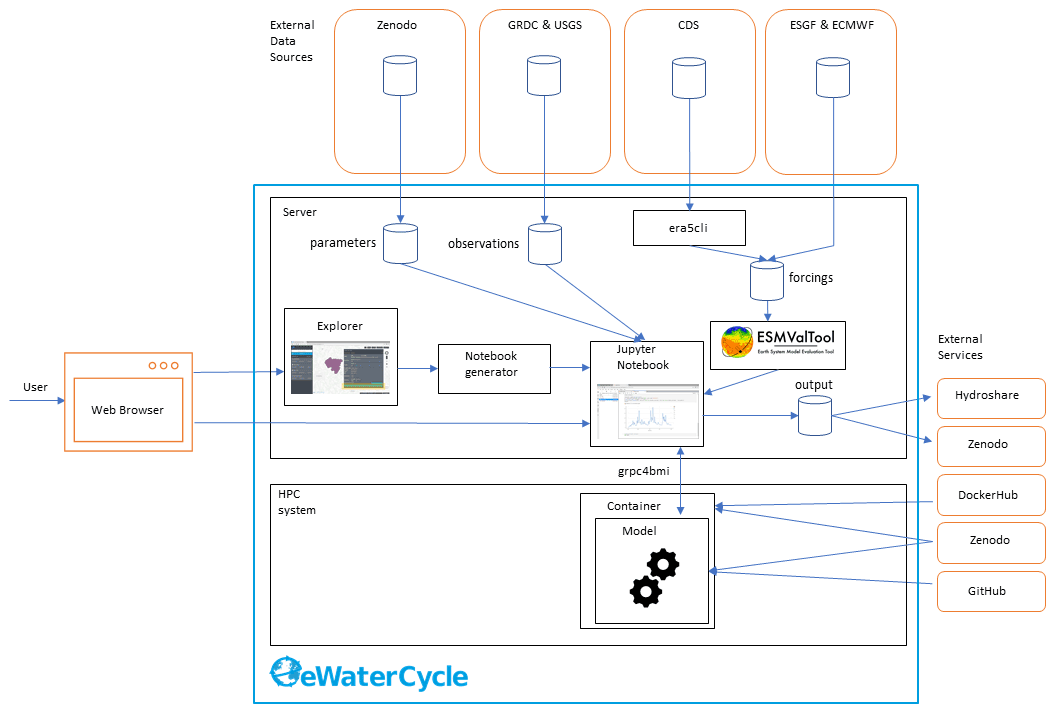
Figure 2 The technological design of the eWaterCycle platform, including external services. This overview shows the different components that are, on purpose, built as separate entities to facilitate reuse in other projects. The different components of this technical overview are discussed in detail in the main text of this publication.

Figure 2 shows the technical design of the eWaterCycle platform. The interface to the system is through a web interface. As the user only needs a web browser to access the eWaterCycle platform, there is no need to install any other software locally, which ensures a low barrier of entry to the system.

The core of the eWaterCycle platform is a collection of services. These are generally deployed on a dedicated server, with ample storage for datasets required to run hydrological models, and to store output. A guide for system administrators on how to install the platform is available in the documentation Verhoeven et al. (2021b). To ensure all data are FAIR, all data in the eWaterCycle platform are downloaded from stable repositories such as Zenodo (general datasets and parameters), the GRDC (runoff observations), ECMWF (ERA-5 and ERA-Interim forcing), and ESGF (Climate Model Data). In addition, required (model) software is downloaded from external sources such as Docker Hub, GitHub and Zenodo.

In turn, the results of experiments done on the eWaterCycle platform can be exported to FAIR data repositories such as Hydroshare and Zenodo. This, together with the FAIR input data, ensures that results generated using the eWaterCycle platform do not depend on the specific server to be sustained indefinitely.

The rest of this section discusses the individual components of the eWaterCycle platform that required significant development effort from the eWaterCycle team. The core of the software stack that runs the eWaterCycle platform has been released as a Python package. Information on how to install this packages and all dependencies is provided in the documentation.

3.1 The explorer

The explorer is a web-based geospatial data explorer for hydrological models and datasets. Using this graphical user interface, users get an overview of the hydrological models available for various regions or catchments and the available datasets at various resolutions. The user can select a combination of models and datasets and configure the experiment they want to set up through this interface.

Figure 3 Screenshots of the explorer, which allows users to explore and select models available based on regions for which they are available (i.e., suitable forcing and parameter sets are available). Background maps are © Microsoft Bing Maps 2018 screenshot(s) reprinted with permission from the Microsoft Corporation.

3.2 The notebook generator

Notebook environments are increasingly popular. They are applied to conduct research, to teach the next generation of hydrologists, for data analysis, and for providing advanced access to large datasets and HPC resources. The notebook generator creates a notebook specifically for the settings chosen by the user, as shown in Fig. 4. The notebook can subsequently be run by the user to perform the requested computation or analysis. In the default use case, the notebook contains the code for running a hydrological model and creating a first hydrograph. Because it is a notebook and not a ready-made user interface with limited options, the user is free to modify the notebook. This method thus allows novice users to get going quickly, while allowing advanced users all the freedom they require. The notebook also forms the perfect basis for a user to start tinkering with the experiment.

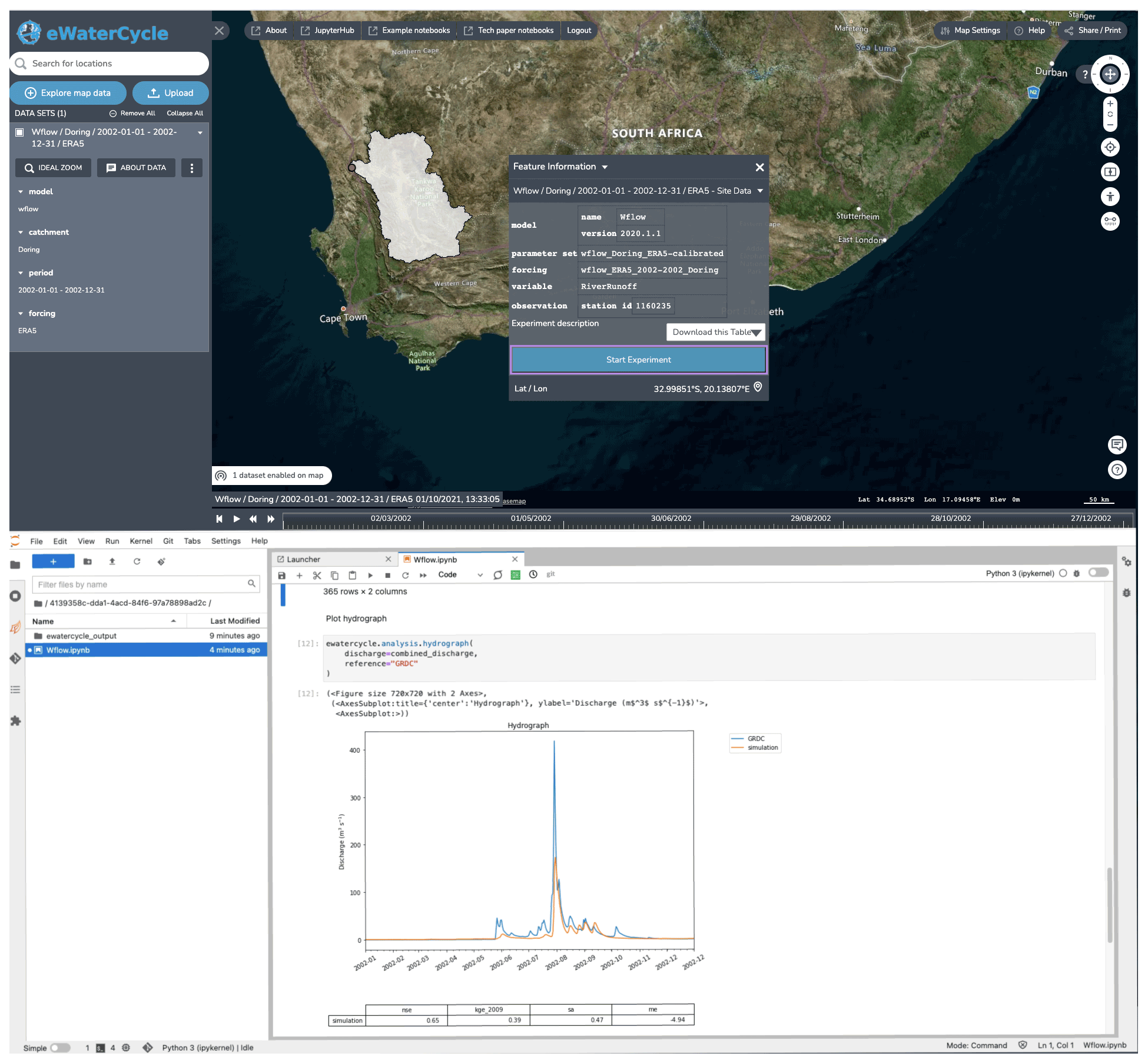
Figure 4 The notebook generator, which generates a notebook based on the experimental setup configured in the explorer. After selecting a model and clicking “start experiment”, a Jupyter notebook is generated and started up that has all the code to, when run, generate a hydrograph for the selected model in the selected region. By providing this working notebook, researchers have a good starting point to change the notebook to answer their own research questions. Background maps are © Microsoft Bing Maps 2018 screen shot(s) reprinted with permission from the Microsoft Corporation.

3.3 Downloading ERA5 with era5cli

With the release of the ERA5 dataset (Hersbach et al., 2020), worldwide high-resolution reanalysis data became available with open access for public use. The Copernicus CDS (Climate Data Store) offers two options for accessing the data: a web interface and a Python API. Consequently, automated downloading of the data requires advanced knowledge of Python. Following our design philosophy of building reusable standalone tools, we have created era5cli to simplify the process of downloading ERA5 data (van Haren et al., 2019). The command line interface tool era5cli enables automated downloading of ERA5 using a single command. All variables and options available in the CDS web form are now available for download in an efficient way. Both the monthly and hourly dataset of ERA-5 are supported. Besides automation, era5cli adds several useful functionalities to the download pipeline, such as spreading a single download over multiple CDS requests and saving files in either GRIB or netCDF. Within the eWaterCycle platform ERA5CLI is used by administrators to download relevant selections from ERA5. Users working in the notebook environment need not work with this command line tool to be able to use eWaterCycle for their research.

Source code is available through van Haren et al. (2019).

3.4 ESMValTool-based model input pre-processor

A large barrier in using a new model or a new dataset for any hydrologist is preparing model input data. In general, this is different for every model as data requirements and data preparations in general differ for most models. The preparation steps are often performed by various sets of scripts that may or may not be included with the model code, which hamper reproducible science. However, there generally is a lot of overlap between the data preparation steps for different models, and as such it would be a valuable asset to the hydrological community if the pre-processing of the input data is done in an open and FAIR manner.

Figure 5 A first hydrograph generated with eWaterCycle. This shows the output of the MARRMoT M01 model (a single bucket representing the entire Merrimack basin) when ERA5 is used as forcing data. While the oversimplification of representing the entire basin with a single bucket is clear, the timing of high-flow periods is still rather well represented. This figure is generated using the hydrograph() function, a standard method within the eWaterCycle package. Next to plotting a hydrograph of the provided time series, it calculates often-used metrics like the Nash–Sutcliffe and Kling–Gupta efficiency values. This example is used as a first “hello world” use case, illustrating with a simple model how the eWaterCycle platform supports standard workflows often used in computational hydrological research.

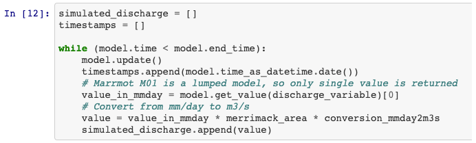
Figure 6 Snippet from the code that generated the hydrograph in Fig. 5. Each time model.update() is called, the eWaterCycle platform instructs the hydrological model running in a container to run for one time step. After each update the user can interact with the state of the model, which in this simple example allows them to extract the calculated discharge at every time step.

To that end, we decided to extend ESMValTool (Righi et al., 2020), a community diagnostic and performance metrics tool for evaluation of Earth system models in CMIP (Eyring et al., 2016), instead of writing model-specific preprocessing scripts. The ESMValTool pre-processing functions cover a broad range of operations on data before diagnostics or metrics are applied, for example, vertical interpolation, land–sea masking, re-gridding, multi-model statistics, temporal and spatial manipulations, variable derivation, and unit conversion. The pre-processor performs these operations in a centralized, documented and efficient way. The current pre-processing pipeline of the eWaterCycle using ESMValTool consists of hydrological model-specific recipes and supports ERA5 and ERA-Interim data provided by the ECMWF (European Centre for Medium-Range Weather Forecasts) through the Climate Data Source (CDS). The pipeline starts with the downloading and CMORization (Climate Model Output Rewriter) of input data. CMORization standardizes the data to make sure that the data are CF-compliant data and follow the CMOR tables. See the ESMValTool documentation for more information on CMORization (https://docs.esmvaltool.org/en/latest/develop/dataset.html, last access: 28 June 2022). Following CMORization, a recipe is prepared to find the data and run the preprocessors. An ESMValTool recipe contains model-specific code to derive forcing variables required by the model, and it will store provenance information to ensure transparency and reproducibility. CMORization is dataset specific and recipes are model specific. This means that after CMORization a dataset is available for all models and a model-specific recipe does not have to be adjusted for a different forcing dataset. Most recipes take a shape file as input, and thus once created it can derive forcing data for any region where data are available in the dataset.

ESMValTool can also be used to pre-process datasets other than ERA5 and ERA-Interim. Examples include climate model results created as part of the Coupled Model Intercomparison Project (CMIP (Eyring et al., 2016)) and distributed through the ESGF platform (Petrie et al., 2021). Our recipes and other additions to the ESMValTool have been merged with the ESMValTool main version. This approach ensures that data preprocessing routines are openly available, documented, and reused.

If hydrologists want to work with their own data sources as forcing for their models within the eWaterCycle platform they can follow the steps on the ESMValTool documentation (https://docs.esmvaltool.org/en/latest/input.html, last access: 28 June 2022) to make their data available. Making their data available for one model, given the way ESMValTool is set up, makes it immediately available for other models as well.

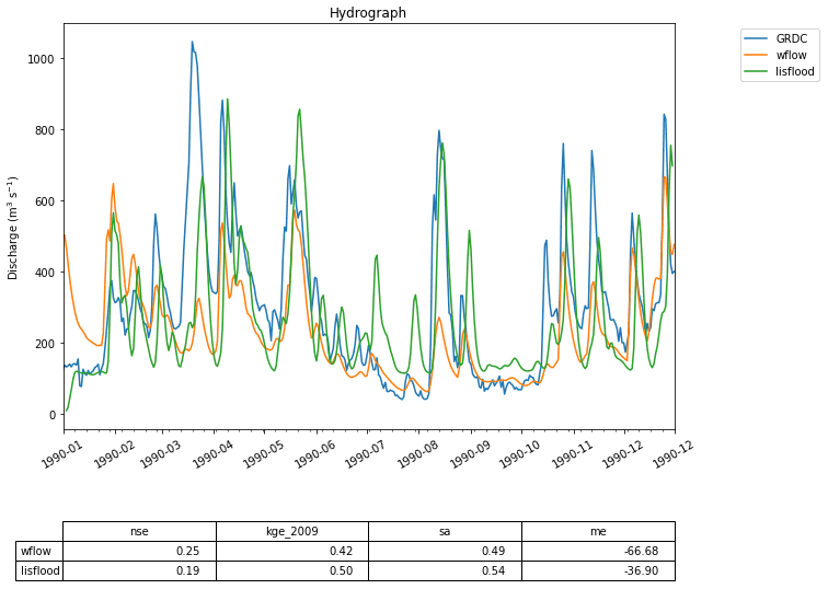
Figure 7 Two hydrographs generated by the Wflow and the LISFLOOD models compared to GRDC observations for the Merrimack basin. While the code used to run these two models given in Fig. 8 is similar to that in the first use case, the models are far more complex and generate better predictions of streamflow.

Figure 8 Snippet from the code that generated the hydrographs of Fig. 7 showing how much this looks like the code of Fig. 6 despite the models involved being far more complex. This shows that the user of the eWaterCycle platform can work with different and complex models from the same environment.

3.5 Interfacing models through grpc4bmi

Hydrological models are written in many different programming languages and often require specific versions of supporting software packages to function as intended by the original model developer. To give hydrologists access to these models without having to learn different programming languages, a common interface to the models is needed. We use the Basic Model Interface (BMI) (Hutton et al., 2020) as our main API for models, which exposes functions for controlling the model time stepping and retrieving and manipulating the model's state at any given moment. BMI is designed specifically to make it easy to implement the interface in any given model. BMI is very forgiving for model structure and is defined for many languages; see https://csdms.colorado.edu/wiki/BMI (last access: 28 June 2022​​​​​​​) for more details. By using GRPC4BMI we can call any model that has implemented BMI from the eWaterCycle platform. We are currently supporting C/C++, Fortran, Octave (open-source version of MATLAB) and R but can add support for any language that has a gRPC library.

To make sure that models are always run using the correct additional libraries and other dependencies, in eWaterCycle models are run inside software containers. A software container is a standard unit of software that packages up code and all its dependencies so that the application runs quickly and reliably on any compute environment. Where model code might break down if a dependency it relies on is no longer supported, packaging a model with its dependencies guarantees that the model can be run on any infrastructure that supports running of containers, thus prolonging the lifetime of the models code base. Communication with a container, for example to instruct a model to run for one time step, happens through well-defined channels that can pass procedure calls. The containers are openly available on Docker Hub or Zenodo to promote reuse by others. In eWaterCycle models written in different programming languages can be added to the platform inside a container, while the Jupyter notebook environment that runs the experiments runs Python. There is, therefore, a need for a tool to translate BMI calls from Python to other programming languages.

To “translate” different BMI versions we have used Google's protocol buffer framework (gRPC) and developed grpc4bmi as standalone software package that allows us to interface codes written in any programming language from our Jupyter notebook environment. Grpc4bmi wraps a BMI-enabled model into a server process, possibly executed within a container and/or on a remote system, and transfers client-side BMI calls to the running model instance. Using gRPC, grpc4bmi establishes the communication between the Jupyter notebook and the hydrological model.

Grpc4bmi allows the user to address model via a standard Python BMI, irrespective of the model's programming language and installation requirements and allows coupling of models and running of multiple instances of the same model. Thus, grpc4bmi serves as a key component of the eWaterCycle platform and is a valuable tool for reproducible analysis and online coupling of BMI-enabled models.

A complete overview of the interface built in eWaterCycle can be found in the documentation at Verhoeven et al. (2021b).

4 Use cases (case studies, application examples)

In this section, we present a number of case studies that illustrate the capabilities of the eWaterCycle platform and the use cases it supports. These illustrate the application of the explorer and notebook generator (Sect. 4.1), how the use of GRPC4BMI allows to switch between different models (Sect. 4.2), coupling models in different programming languages (Sect. 4.3), performing experiments on a model's internal state while the model is running (Sect. 4.4), and calibrating a model using a remotely executed ensemble (Sect. 4.5).

The case studies presented here are chosen to demonstrate the features of the platform in a clear way. They all feature only a single catchment. Current hydrological modeling studies often include many catchments in their analysis. The platform fully supports those more complex studies, as is shown in Aerts et al. (2021), where the impact of different spatial resolutions of the same model are studied for 454 catchments from the CAMELS dataset.

All figures presented with these use cases are generated with the eWaterCycle platform and have not been optimized for printing to show what the output of experiments done with eWaterCycle looks like. The Jupyter notebooks for these use cases are provided in a separate GitHub repository to facilitate adding additional notebooks at later stages. For the exact notebooks used in this study, a release with associated DOI has been made (Hut et al., 2021).

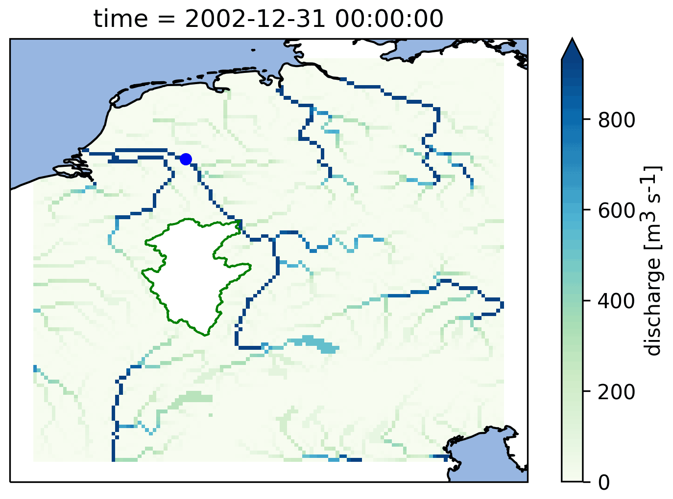
Figure 9 Calculated discharge in the Rhine basin at the end of the model run using the PCR-GlobWB 2.0 model for the Rhine coupled with the simplest one-bucket model from the MARRMoT suite of models for the Moselle subcatchment. The Moselle subcatchment has been cut out of the PCR-GlobWB 2.0 model (by altering its “landmask” setting). MARRMoT calculates the discharge for the Moselle, and at each time step this is added to the “channel storage” parameter of PCR-GlobWB 2.0 at the location where the Moselle flows into the Rhine (at Koblenz). The blue dot on the map indicates the location of the observation station at Lobith, which is used for the hydrographs shown in Fig. 11.

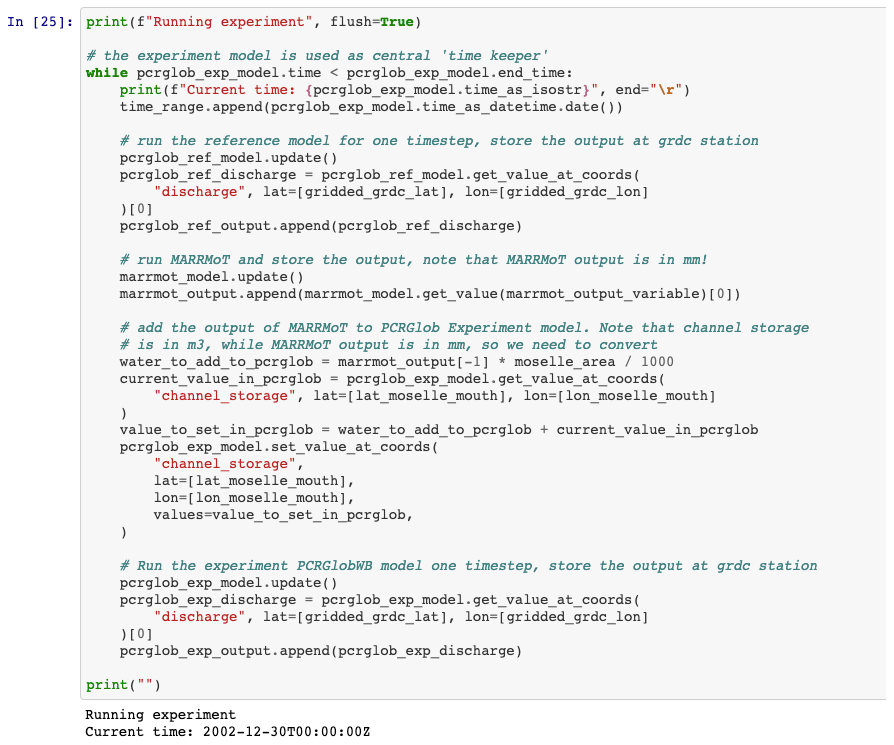
Figure 10 The central loop of the experiment presented in Sect. 4.3. Within the loop three models are run: MARRMoT for the Moselle sub-basin and two instances of PCR-GlobWB 2.0. The first, called “reference”, runs the entire Rhine basin without alteration. The second, called “experiment”, runs the Rhine basin with the Moselle subcatchment cut out (by altering the landmask file). At every time step the discharge calculated by MARRMoT for the Moselle is added to the “channel storage” variable of PCR-GlobWB 2.0 at the mouth where the Moselle enters the Rhine (at Koblenz). This code snippet shows how the eWaterCycle platform supports model coupling without having to interfere with the code of the models being coupled.

4.1 Hello world: one model, one catchment, one forcing

Our first application is the most basic notebook that is produced by the notebook generator after configuring the experiment in the explorer. This notebook includes all the code and configurations needed to download and pre-process model input data and forcing data from ERA5. After pre-processing is finished, the code to set up, initialize and run the model while capturing discharge estimates is given. Finally, there is code to download observation data from GRDC for the corresponding GRDC station and plot a hydrograph of both the modeled and observed discharge over the simulated period, as shown in Fig. 5.

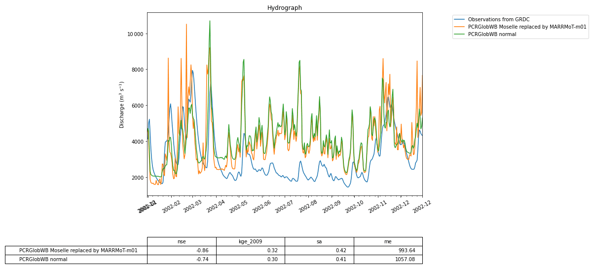
Figure 11 The calculated discharge for the Rhine basin from PCR-GlobWB 2.0 when run normally (i.e., the reference) and when coupled with MARRMoT for the Moselle subcatchment. The calculated discharge is compared to GRDC observations of discharge.

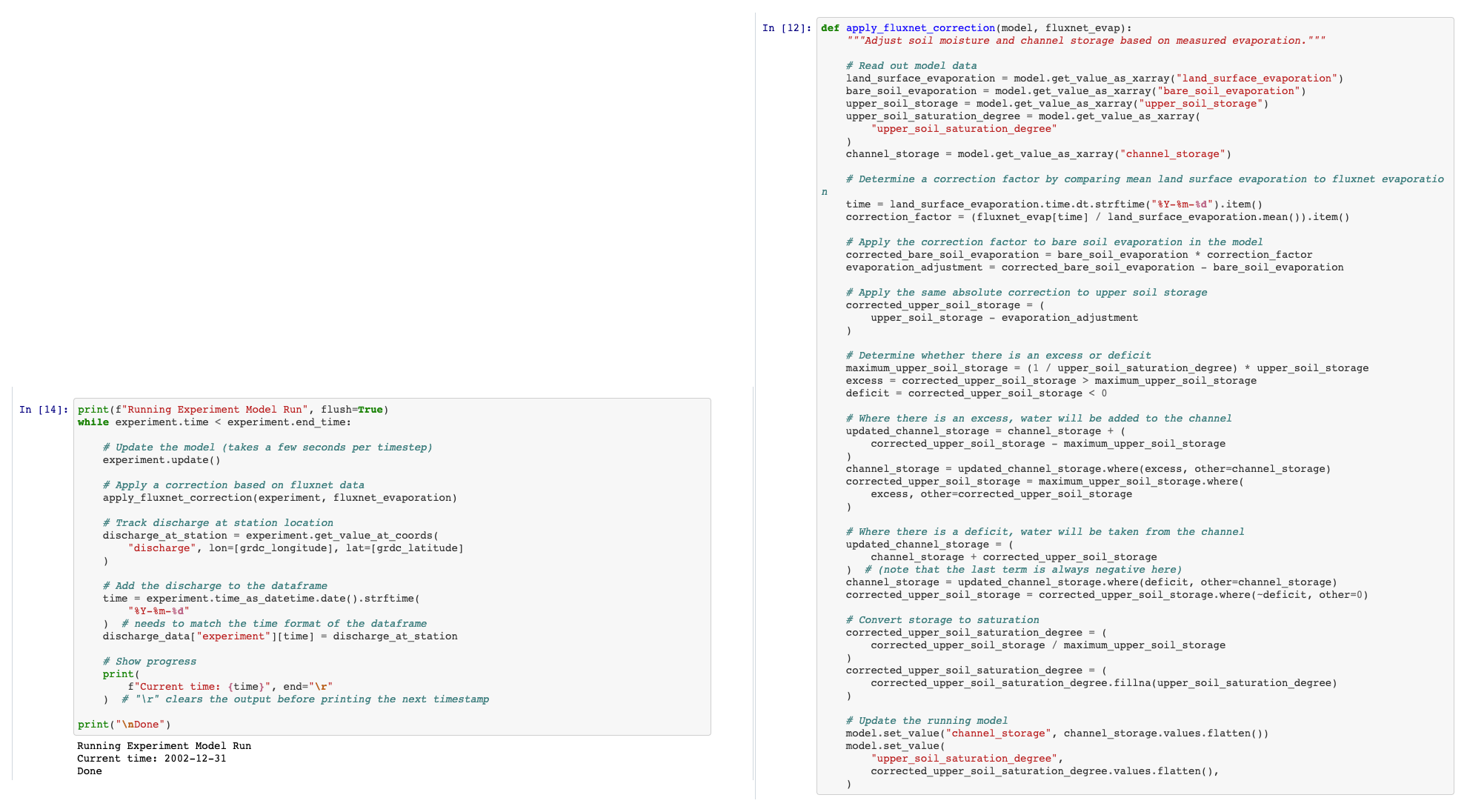
Figure 12 The code used to interfere with the state of PCR-GlobWB 2.0 during runtime. This code is available through Hut et al. (2021) (https://doi.org/10.5281/zenodo.5543899). Each time step the function apply_fluxnet_correction() is called. The right-hand side of this figure shows the code of that function. The model.get_value_as_xarray() called at the start of the function extracts information on the state from the model. The model.set_value() called at the end of the function updates the state with the newly calculated information. This example shows that numerical hydrologists can interact and experiment with the state of a hydrological model without having to interact with the code of the model. In this way a clear separation between model and experiment is achieved.

For this specific example, we have chosen to use the MARRMoT (Knoben et al., 2019) model suite. MARRMoT is a suite of conceptual catchment models written in the MATLAB programming language where the user can specify the model structure through setting files. In eWaterCycle, these setting files are generated when the model instance is created. Specific settings, such as the maximum soil moisture storage in this case, can be set by the user in the notebook. Here we have chosen the most basic model available: a single bucket. Figure 6 shows the central part of the notebook where the model is run. As catchment, the Merrimack basin is chosen and ERA5 is used as forcing dataset. While the Merrimack is too large and complex of a basin to be represented by such a simple model, this “hello world” example shows that in eWaterCycle any model, whether lumped or distributed, can be run using any available forcing dataset for any region. To run this model for any other region the only change a user needs to make is to provide another shapefile and select another GRDC observation station.

This first use case shows that a model written in a completely different programming language can be run in eWaterCycle without having to understand, install, or even be aware of the model code. In this example, the parameters for the single bucket model in MARRMoT were chosen by the user. Normally, conceptual models, such as MARRMoT, need to be calibrated; see Sect. 4.5 below for a use case demonstrating how to calibrate a hydrological model within eWaterCycle.

Figure 13 This graph shows the effect of interfering with the state of the PCR-GlobWB 2.0 model. The calculated discharge for the Merrimack basin from two model runs is shown: one reference where the model is run without interfering and one experiment where at every time step the state of the model is changed to incorporate evaporation observation data from Fluxnet (Pastorello et al., 2020). The calculated discharge for both model runs is compared to GRDC observations of discharge.

4.2 Model comparison: two models, one catchment, one forcing

In hydrological modeling, an important decision is which model to use for answering a specific research question¹. To this end, hydrologists want to compare two or more models with identical forcing to evaluate the differences in model behavior and performance.

Figure 7 shows the result of such an experiment, where simulated discharge estimates produced by wflow and LISFLOOD are evaluated against GRDC observations at the Merrimack basin outlet. As Fig. 8 shows, the code used in the notebook to run the two models is nearly identical to that of the first use case from Sect. 4.1 thanks to the uniform way in which models are interfaced within the eWaterCycle platform. This significantly reduces the effort involved in comparing different models and stimulates objective model selection based on adequacy for answering a particular research question.

The code in this notebook can be adapted to run a selection of available models by changing which container is started on any region supported by those models, using any input forcing dataset available on the platform. Changing a forcing dataset is done by passing another forcing object to the model upon creation of the model instance. In practice this means as little as changing a string in the Jupyter notebook describing the experiment from for example “ERA-Interim” to “ERA5”. Hydrologists use this to determine which model to use to answer their research question. Consultants and policy makers can use this to, for example, determine which model to use for future projections of the impact of climate change on local hydrology. Operational water managers can use this to determine which model to use in their operational forecasting systems.

4.3 Model coupling: add output of one model as input for downstream model

As a consequence of the curse of locality mentioned in Sect. 1, different regions often have a different model that behaves best for a particular research goal. However, technological differences between the implementations of these models currently prevent researchers from coupling different models for different regions into a larger patchwork of multi-models. The eWaterCycle platform removes such technological barriers and enables users to couple models written in entirely different programming languages.

As an example, we demonstrate how discharge calculated by the simplest one-bucket model from the MARRMoT suite of models for the Moselle River (a subsidiary of the Rhine) is inserted into the PCR-GLOBWB 2.0 model, which is simulating the rest of the Rhine basin. Figure 9 shows a map of the calculated discharge in the Rhine basin with the Moselle subcatchment on top of it. We have cut out the Moselle subcatchment from the PCR-GLOBWB 2.0 model, and at every time step the discharge as calculated by MARRMoT is added to the channel storage variable where the Moselle enters the Rhine. As a reference, we also run the PCR-GLOBWB 2.0 model for the whole Rhine basin without coupling to MARRMoT.

Figure 14 A snippet of the code used to run the calibration experiment described in Sect. 4.5. The entire workflow of the first use case presented in Sect. 4.1 is wrapped into the function run_model() (left part of the figure). This function runs the model for a given set of parameters. This function is called in objective_function(), which is passed as an argument to the calibration scheme of the CMA-ES/pycma package. This package, based on settings provided, runs multiple instances of the objective_function() (and thus of the hydrological model) in parallel to find the optimum set of parameters that optimize the objective function.

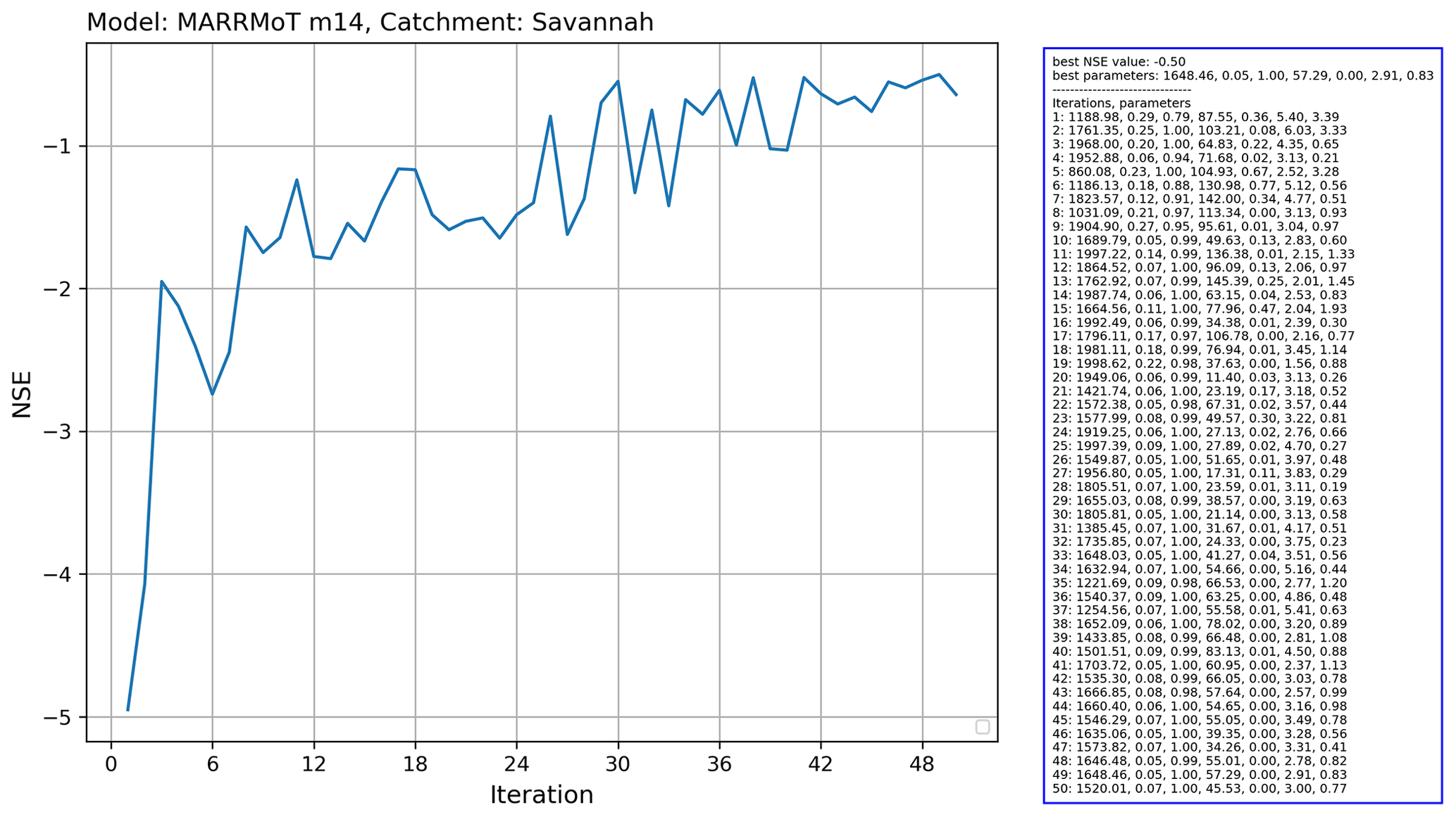
Figure 15 Output of the running the Covariance Matrix Adaptation Evolution Strategy (CMA-ES) calibration scheme from the CMA-ES/pycma software package on the MARRMoT m14 model (an implementation of TOPMODEL) for the Savannah basin.

Figure 10 shows the central loop of this coupling experiment. Within the loop, the following three models are run: MARRMoT for the Moselle sub-basin and two instances of PCR-GlobWB 2.0. The first, called “reference”, runs the entire Rhine basin without alteration. The second, called “experiment”, runs the Rhine basin with the Moselle subcatchment cut out (by altering the landmask file). During every time step the discharge calculated by MARRMoT for the Moselle is added to the “channel storage” variable of PCR-GlobWB 2.0 at the mouth where the Moselle enters the Rhine (at Koblenz). This code snippet shows how the eWaterCycle platform supports model coupling without having to interfere in the code of the models being coupled. While this example shows the coupling of two hydrological models, the eWaterCycle platform facilitates coupling of any models that incorporate a Basic Model Interface (BMI), including those not describing hydrology. Work where hydrological models are connected to, for example, models describing human behavior (Elshafei et al., 2015) or geomorphological processes (Hancock and Willgoose, 2001) can be done using the eWaterCycle platform.

Figure 11 shows the discharge computed by the coupled models and the reference model. The impact of using a conceptual model can clearly be seen in the different model outputs. Note that in this example the two models are written in different programming languages (MATLAB for MARRMoT and Python for PCR-GLOBWB 2.0). While the experiment formulated in the Jupyter notebook is also written in Python, it does not interact directly with the code of the models, meaning that all interaction happens through grpc4bmi.

4.4 Model interaction: change state of model during runtime

Hydrological models are great tools for “what if” type research questions such as “What is the impact on river discharge downstream if the land use upstream is changed?”. These types of research questions often require direct interfering in the state of the model (with “state” as defined in the glossary). Previously, this meant having to adapt the model code to reflect the required research question, leading to a new version of the model. Using the eWaterCycle platform, model variables are exposed through BMI and can be queried or set without changing the model source code itself. This separates the “experiment” from the hydrological model used to conduct the experiment with.

In this example use case, we answer the following research question: “What would happen to the prediction of discharge when we, instead of calculating evaporation, use observations for evaporation?”. At every time step the soil storage variables in the PCR-GLOBWB 2.0 model are changed based on Fluxnet (Pastorello et al., 2020) observations. Hydrologically relevant choices for this experiment, such as “what to do if the observations state that more water is evaporated than is available in the soil storage” are now implemented as part of the experiment and not as changes to the model source code, as shown in Fig. 12. This increased transparency and separation of experiment and model makes it easier to repeat the experiment with different models and to understand and build upon each other's work.

Figure 13 shows the calculated river discharge at the basin outlet for both the reference run (with no interference in the model) and the experiment run. The impact is clearly visible; the discharge estimates of PCR-GLOBWB 2.0 become worse when the model is constrained with observations of evaporation. This leads to a host of follow-up questions. Is the evaporation measurement used representative for the (entire) catchment? Does the calculated evaporation compensate for missing fluxes in other parts of the model? Finally, this experiment is part of the thesis work of BSc student Thomas Albers (Albers, 2020), illustrating that by using the eWaterCycle platform students can focus on hydrologically interesting research questions without having to invest a large amount of time to learn and modify a particular model's source code.

4.5 Calibrating a model using an ensemble of model runs

Many hydrological models have parameters that need to be calibrated before a model can be used. A whole subfield of hydrology has formed around the research question of what the best, most efficient or robust way is to calibrate a model (Bárdossy, 2007; Bárdossy and Singh, 2008). These calibration methods typically require an ensemble of models as part of the optimization process. The eWaterCycle platform supports transparent and efficient calibration of hydrological models through the separation of model and experiment, as well as the ability to run models in containers on remote machines.

In this example, we calibrate the MARRMoT m14 model (an implementation of TOPMODEL), which has seven free parameters for the Savannah basin. We used the Covariance Matrix Adaptation Evolution Strategy (CMA-ES) calibration scheme, which is provided by the CMA-ES/pycma software package (Hansen et al., 2021). The model runs were done on the Cartesius supercomputer. Figure 14 shows a snippet of the code that shows the clear separation between model and calibration routine.

The results for this calibration experiment are shown in Fig. 15. The increase in objective function shows the convergence of the algorithm. This use case shows that separation of model and experiment makes calibration of hydrological models easier to set up with eWaterCycle.

5 Conclusions

We have introduced the eWaterCycle platform for FAIR and open hydrological modeling. Using eWaterCycle, hydrologists can easily build on each other's work by using each other's models, data and experiments in a manner that is “FAIR by design”. Using the online eWaterCycle platform, hydrologists do not have to install, download or pre-process anything before they can start computational hydrological experiments.

The eWaterCycle platform implements the “FAIR” principles as follows.

• Findable. The data and models must be findable. Through the explorer, all available models and datasets are exposed in an easily findable manner. The documentation (Verhoeven et al., 2021b) further specifies all available models, datasets and their properties.

• Accessible. The data and models must be accessible. By making the entire software-stack of the eWaterCycle platform open source and by only including models and datasets that are also openly available, it is possible for anyone with sufficient computational infrastructure to install and run an instance of the eWaterCycle platform. For those without these resources, the eWaterCycle team (i.e., the authors of this paper) currently hosts an instance of the eWaterCycle platform on demonstration hardware provided by SURF. Access to this version can be obtained through contact with the authors. In the near future, the eWaterCycle team is hoping to acquire funds to more sustainably offer an instance of eWaterCycle to the entire hydrological community.

• Interoperable. The data and models must be interoperable. The eWaterCycle platform uses open interfaces between the different parts of the platform (e.g., grpc4bmi) to communicate between experiments in Jupyter notebooks and the hydrological models in containers. The use of open interfaces and containers makes it easy to connect to a dataset or a model and use it for a different study.

• Reusable. The data and models must be reusable. The experiments in eWaterCycle, as contained in Jupyter notebooks, are separate entities from the models and datasets. Because of this separation and the open interfaces between components, reuse of data, models or (parts of) experiments is facilitated.

As laid out in Sect. 1, currently an ecosystem of services is emerging that makes it easier for hydrologists to do computational research, with each service focusing on different parts of the hydrological research cycle (Tucker et al., 2022; Tarboton et al., 2014). In this ecosystem, eWaterCycle is developed as a platform on which hydrologists can execute their computational hydrological experiments. In this paper, we have presented the core components of the eWaterCycle platform, the explorer, the notebook environment, and the underlying technology to deal with models and datasets in a FAIR manner. The hydrological community can install the openly and freely available eWaterCycle platform on their own infrastructure. The eWaterCycle team (i.e., the authors of this paper) are attracting sustainable funding to provide an online place where more researchers will be able to execute their computational hydrological research and education.

For future development, integration with other platforms that facilitate hydrological research is foreseen, most notably coupling to models from CSDMS, sharing and retrieving data from Hydroshare, integrating higher-level interfaces to models, such as PyMT, and giving access to libraries that facilitate additional types of research such as the data assimilation software OpenDA.

The use cases presented in this paper give an overview of the type of research that the eWaterCycle platform can facilitate, from model selection to coupling and calibration. The eWaterCycle platform is set up as a modular collection of services that together form a complete platform. By making sure that the individual modules contain as few assumptions about hydrology as possible (those are represented in the models and experiments), we are working towards the goal of making the technologies developed for the eWaterCycle platform portable to other domains of (geo)science where researchers work with each other's models and datasets.

Hutton et al. (2016) argued that computational hydrology can only be a proper science if the hydrological community makes sure that hydrological model studies are executed and presented in a reproducible manner. We replied that to improve current practices for hydrologists using hydrological models in their work, hydrologists should not “re-invent the water wheel” but instead use existing technology from other fields, such as containers and the ESMValTool, and open interfaces, such as BMI, to do their computational science (Hut et al., 2017). With this paper and the release of the eWaterCycle platform, we are putting our money where our mouth is and providing the hydrological community with a “FAIR by design” platform to do science.