the Creative Commons Attribution 4.0 License.
the Creative Commons Attribution 4.0 License.
 | 07 Jul 2022
Evaluating the Atibaia River hydrology using JULES6.1
Ana Maria Heuminski de Avila
Michaela Bray
Land surface models such as the Joint UK Land Environment Simulator (JULES) are increasingly used for hydrological assessments because of their state-of-the-art representation of physical processes and versatility. Unlike statistical models and AI models, the JULES model simulates the physical water flux under given meteorological conditions, allowing us to understand and investigate the cause and effect of environmental changes. Here we explore the possibility of this approach using a case study in the Atibaia River basin, which serves as a major water supply for metropolitan regions of Campinas and São Paulo, Brazil. The watershed is suffering increasing hydrological risks, which could be attributed to environmental changes, such as urbanization and agricultural activity. The increasing risks highlight the importance of evaluating the land surface processes of the watershed systematically. We explore the use of local precipitation collection in conjunction with data from a global meteorological reanalysis to simulate the basin hydrology. Our results show that key hydrological fluxes in the basin can be represented by the JULES model simulations.
- Article
(913 KB) - Full-text XML
- BibTeX
- EndNote


The Atibaia River basin serves as a major water supply for Campinas and São Paulo (Demanboro et al., 2013; Nobre et al., 2016). The basin is subjected to human impacts such as urbanization and agricultural activities. Increasing hydrological risks have emerged with historic floods in 2009 and 2010 (Campos and Carneiro, 2013), and drought in 2014 and 2015 (Marengo et al., 2015; Nobre et al., 2016), which highlight the importance of evaluating the hydrology systematically. Hydrological models are an essential tool in hydrological science and catchment management for evaluating the hydrological impacts of climate change or land-use and land-cover change (Buytaert and Beven, 2011). There have been several recent research activities centered on the Atibaia River basin (dos Santos et al., 2020; Prochmann, 2022) due to its importance in the water supply.
Physically based hydrological models are often used to simulate the physical water flux under given meteorological conditions, allowing us to understand and investigate the cause and effect of environmental changes. One such physically based model, commonly used, is the Soil Water Assessment Tool (SWAT), which has been used for flow and sediment estimation for the Atibaia River basin (dos Santos et al., 2020). However, the accuracy of the model highly depends on the model structure as well as the availability and quality of input data. Also, local calibration is usually required due to the few empirical approximations in each model.
The JULES model was developed from the Met Office Surface Exchange Scheme (MOSES) by the UK Met Office (Cox et al., 1999). It can be coupled to an atmospheric global circulation model but is also used as a standalone land surface model that simulates the carbon fluxes (Clark et al., 2011), water, energy, and momentum (Best et al., 2011) between the land surface and the atmosphere. The model is driven by a large dataset of meteorological variables using a physically based approach and has been increasingly used for hydrological assessment (Le Vine et al., 2016; Martínez-de la Torre et al., 2019; Zulkafli et al., 2013). Therefore, we examine the model's ability to simulate the land surface processes of the Atibaia watershed.
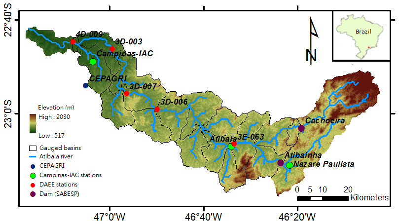
Figure 1Atibaia River basin and the location of the weather stations, flow monitoring stations, and dams.
2.1 Study region and data
This study explores the hydrology of the Atibaia River basin. The altitude of the catchment ranges between 517 and 2030 m; it is located between the coordinates 22∘40′ and 23∘30′ S and 47∘30′ and 46∘00′ W in southeastern Brazil, covering an area of 2816.4 km2 (Fig. 1). For 18 sub-basins, the surface (Qsurface) and sub-surface (Qsubsurface) runoff fluxes are simulated with rainfall data from the monitoring station (Campinas, Atibaia, and Nazare Paulista) of Campinas Agronomic Institute (Campinas-IAC) and from the station of the Department of Water and Electricity (DAEE, 2022). The modeling results cover 1999.2 km2 effectively since the Cachoeira Dam and the Atibainha Dam intercept the upstream flow, and the monitoring station does not cover part of the lower basin. The released data of the dams are used as the upstream flow, which is obtained from the Sao Paulo State Sanitation Company (SABESP, 2022). River flow observations from three stations (4D-009, 3D-006, 3E-063) measured by DAEE (2022) are used for model calibration and validation.
The primary soil types in this area are Ferralsols, Acrisols, Leptosols, and Cambisols (FAO/IIASA/ISRIC/ISSCAS/JRC, 2012; Ottoni et al., 2018; Rossi, 2017). The required soil parameters are obtained by using the pedotransfer functions (PTFs) of Hodnett and Tomasella (2002), which generate parameters from physical and chemical properties of soil obtained from a large-scale soil database at 0.083∘ resolution (FAO/IIASA/ISRIC/ISSCAS/JRC, 2012). The primary land cover is rural (53.0 %), followed by forest (27.6 %), and then urban (12.0 %). Higher percentages of forest are found in the upper basin, whereas urban areas concentrate in the lower basin. We classified the land cover into five vegetated plant functional types (Harper et al., 2018), including tropical broadleaf evergreen trees (BET-Tr), needle-leaf evergreen trees (NET), C3 grasses (C3), C4 grasses (C4), evergreen shrubs (ESH), and two non-vegetated types: bare soil (BS) and urban (U) using MODIS data (Friedl and Sulla-Menashe, 2015) and reclassified by Houldcroft et al. (2009).
The study region's rainfall presents a seasonal pattern with rainy summers and dry winters (Cavalcanti et al., 2017; Dias et al., 2013). The rainfall regimes are influenced by the passage and frontal systems' intensity (Maddox, 1983; Silveira et al., 2016). The maximum precipitation occurs during the austral summer associated with the South Atlantic Convergence Zone (SACZ) and in the winter the high pressing system of the South Atlantic is predominant (Jones and Carvalho, 2013). For this study, rainfall time series from 2009 to 2019 are provided by three stations from Campinas-IAC and five stations from DAEE (Fig. 1). The missing rainfall records are completed with the records from a neighbor using multi-regression. The temperature, specific humidity, and surface pressure are observed by the Center for Meteorological and Climate Research Applied to Agriculture (CEPAGRI). The air temperature is elevation-adjusted with the lapse rate (γ) 1.4 ∘C per 100 m obtained from Campinas-IAC and CEPAGRI data during the study period.
Table 1Sensitivity analysis of hydrological parameters using (1) PDM and (2) TOPMODEL. Default parameter values are in bold.
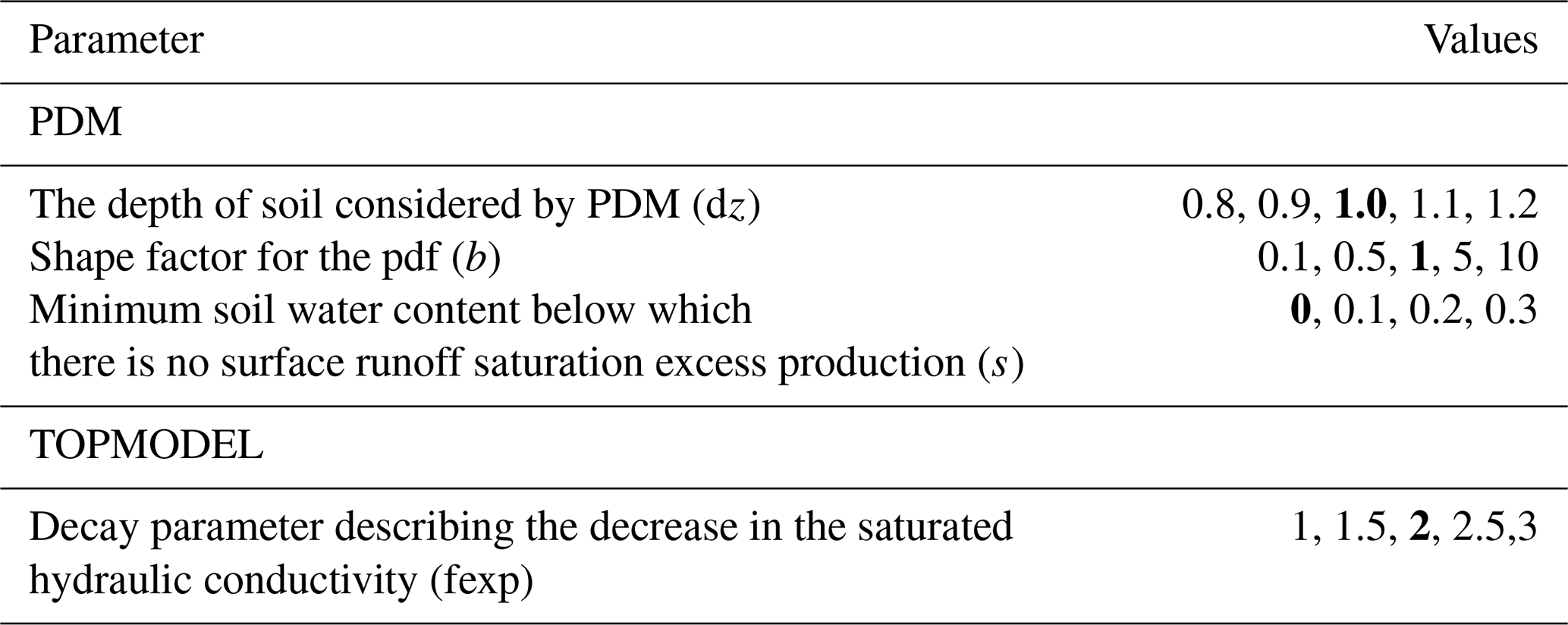
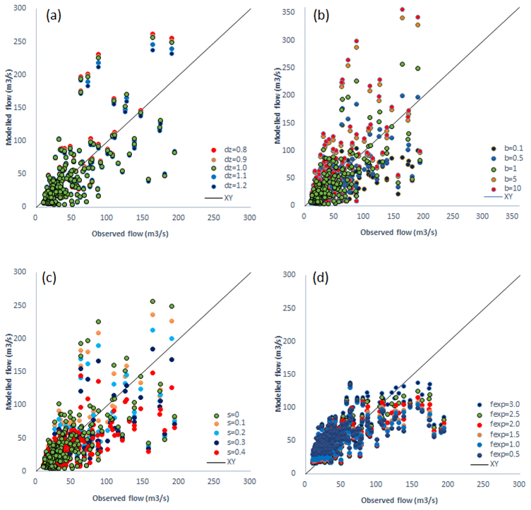
Figure 2Sensitivity analysis of daily mean flow in the lower basin with (a) soil depth, (b) shape factor, and (c) threshold of minimum soil water content, using PDM, and (d) decay parameters, using TOPMODEL.
Other meteorological data required include downward short-wave radiation, long-wave radiation, and wind speed, all of which are extracted from the NCEP-DOE Reanalysis II dataset (Kanamitsu et al., 2002). The dataset is available on a T62 Gaussian grid with 192×94 points (approximately 2∘ scale) and provides a 6-hourly temporal resolution from January 1979 up to the present. The 6-hourly resolution was disaggregated into hourly data using linear interpolation.
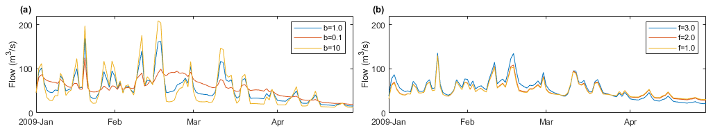
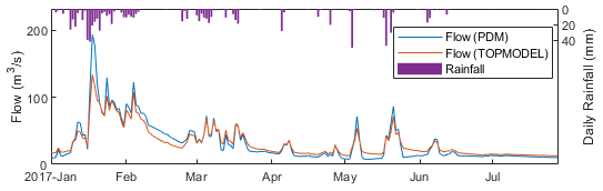
Figure 3Daily modeled flow in the lower basin using different (a) shape factors (PDM), (b) decay parameters (TOPMODEL).
2.1.1 The JULES model
JULES simulates the energy exchange between different land surface processes described by Best et al. (2011) and Clark et al. (2011). For each sub-basin, distinct parameters are used to calculate the energy balance of surface temperatures, short-wave and long-wave radiative fluxes, sensible and latent heat fluxes, ground heat fluxes, canopy moisture contents, snow masses, and snow melting rates for each surface type in a grid box. The sub-grid surface heterogeneity is described using a tiled model upon a shared four-layer soil column with a thickness of 0.1, 0.25, 0.65, and 2.0 m from top to bottom. In JULES, precipitation is intercepted by the canopy storage, and then throughfall is then partitioned into surface flow and infiltration into the soil based on the Hortonian infiltration excess mechanism. JULES incorporates one of two different hydrologic models: (1) Probability Distributed Model (PDM) described by Moore (1985) and (2) TOPMODEL described by Beven and Kirkby (1979). In our model setup, we have calculated saturation excess flow by first using the PDM, with the sub-grid distribution of soil moisture (θ) described by a probability function (Clark and Gedney, 2008). The saturated fraction (fsat) is described as follows:
S is the areal fraction of grid-box soil water storage. S0 is the minimum soil water content below which there is no surface runoff saturation excess production by PDM. Smax is the maximum grid-box storage, which is equal to the volumetric soil water content (θs) multiplied by the soil depth (Zpdm). The shape parameter (B) is initially set as 1, whereas an alternative value of 0.1 or 0.5 can be used to better represent a more subsurface-flow-dominated hydrology, and a value of 10 to represent a more flash hydrological response. For the TOPMODEL approach, the saturated fraction (fsat) is found by integrating the probability distribution function (pdf) of the topographic index (λ). Numerical integration using a two-parameter gamma distribution can be found in Gedney and Cox (2003) as follows:
in which as and cs are fitted parameters for each sub-basin, λic is the critical value of the topographic index at which the water table reaches the surface, and f is a decay parameter describing the decrease in the saturated hydraulic conductivity. The mean value and standard deviation of the topographic index data are obtained from Marthews et al. (2015).
For both PDM and TOPMODEL, precipitation over the saturated fraction of the grid generates surface runoff. An instantaneous redistribution of soil moisture is assumed for the infiltration following the Darcy–Richards diffusion equation. The gravity drainage generates the subsurface flow at the lower boundaries.
We evaluated the sensitivity of modeled streamflow to the hydrological parameters shown in Table 1 and calibrated the model to select the most suitable approach for the study region. Soil hydraulic characteristics are estimated using the relationship of Van Genuchten (1980).
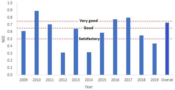
Figure 5NSE score of modeling daily flow in the lower basin using TOPMODEL summarized by year.
2.2 Model evaluation
The runoff fluxes simulated by the JULES model require an external river routing model for a reasonable comparison to observed river flows (Best et al., 2011). In this study, we applied a simple delayed function to account for the routing delay in the modeled flow (Qsim) in each time step (t). Following the routing process, the flow (Qrout) aggregated from each sub-basin (n) in the outlet is as follows:
The delay time (ti) for each sub-basin is given by dividing the distance from the sub-basin to the outlet (di) by flow speed (C), which is set constantly as the average flow speed of 0.40 m s−1 (from 2009 to 2019).
We evaluated the sensitivity of hydrological parameters of PDM and TOPMODEL to determine the most suitable model in the upper (3E-063), middle (3D-006), and lower basin (4D-009) using the simulated results from the first year. Soil depth (dz_pdm), shape factor (b_pdm), and the fraction of maximum storage (s_pdm) are evaluated for PDM, and a decay parameter describing the decrease in the saturated hydraulic conductivity (f) for the TOPMODEL. Following the sensitivity analysis, the full model is run with the parameter combination with the highest Nash–Sutcliffe efficiency (NSE) performance. We evaluated the overall model performance over the modeling period (N) using the NSE, RMSE-observation standard deviation ratio (RSR), and percent bias (PBIAS), following Moriasi et al. (2007), where Qobs, mean is the mean of observed flow, and Qobs,t and Qmod,t are the observed flow and modeled flow at a daily time step (t).
3.1 Sensitivity analysis
We evaluated the sensitivity of hydrological parameters in PDM and TOPMODEL. For PDM, we found lower flow simulated with increasing soil depth (Fig. 2a). However, the average flow only reduced by 2.5 % when soil depth was increased from 0.8 to 2.0. In contrast, we found that the shape factor (Fig. 2b) and minimum soil water content (Fig. 2c) had a higher impact on the simulated flow. When we increased the minimum soil water content, the simulated flow was reduced with more water held in the soil. The average flow was reduced by 17.5 % when the minimum soil water content increased from 0 to 0.4, whereas gradual changes were found in the flow regime. For the shape factor, a lower value simulates a more gradual flow regime (Clark and Gedney, 2008), which in turn lowers the peak level flow estimation and hence increases baseflow generation (Fig. 2b). In this case, the shape factor (b=0.1) can change the flow into a subsurface-flow-dominated regime (Fig. 3a). We found that the shape factor of 0.5 best describes the flow in the study basin.
We examined the model performance with a combination of soil depth, shape factor, and the minimum soil water content and found the highest performance with the combination dz=1.0, b=0.5, and s=0 in the lower basin, which altered the shape factor alone from the default setup. In the middle and upper basin, an increased value of the minimum soil water content simulated higher performance (dz=1.0, b=0.5, s=0.1). Therefore, we run the full-time series of modeling with these parameter combinations.
For the TOPMODEL, we found that the lower decay parameter increases the baseflow (Figs. 2d, 3b) and reduces the magnitude of peak flows. In terms of model performance, we found a value of f=3.0 simulates the flow in the lower and middle basin well, whereas a lower value of f=2.0 is more suitable in the upper basin. These values were then selected to be used for the full model simulation.
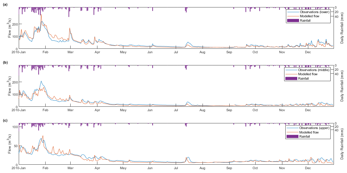
Figure 6Daily modeled flow, observed flow, and rainfall in the (a) lower, (b) middle, and (c) upper basin in the year 2010 using TOPMODEL.
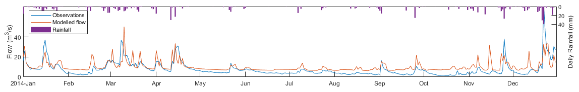
Figure 7Daily modeled flow, observed flow, and rainfall in the lower basin in the year 2014 using TOPMODEL.
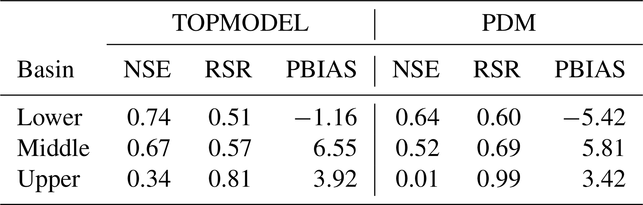
Table 2Modeling performance as calculated from the observed and modeled flow time series in lower, middle, and upper basins, using (1) TOPMODEL and (2) PDM. NSE: Nash–Sutcliffe efficiency. RSR: RMSE-observation standard deviation ratio. PBIAS: percentage of bias.
3.2 Hydrological modeling using the JULES model
Table 2 summarizes the evaluation of the JULES model in the upper, middle, and lower basin. For the entire basin (lower), the TOPMODEL shows “good” modeling performance (0.75 > NSE > 0.65, 0.6 > RSR > 0.5), and the PDM shows “satisfactory” modeling performance (0.65 > NSE > 0.50, 0.7 > RSR > 0.6) (Moriasi et al., 2007). Figure 4 shows that lower peak flow and higher baseflow is simulated using TOPMODEL, which is more suitable for our study basin. In the middle basin, both models are marked as having “good” performance. “Unsatisfactory” is marked for both TOPMODEL and PDM in the upper basin. We attributed one possibility to the rainfall data recorded in the upper basin. Although the difference in the average annual rainfall is below 4 % in the whole basin, the variation might be not well represented in the upper basin. However, TOPMODEL still simulates an acceptable result (NSE > 0.15) for daily flow simulation considering the difficulty and high variation at daily time step (dos Santos et al., 2020). In terms of average flow, the bias is marked as “very good” (PBIAS<10) for all the simulations.
Figure 5 shows the modeling performance of daily flow in the lower basin yearly using TOPMODEL. The modeling performance is marked as “very good” in 3 years, “good” in 1 year, and “satisfactory” in 4 years, with the overall performance marked as “good”. The highest modeling performance is simulated in 2010 (NSE = 0.89), whereas a lower score is simulated in 2014 (NSE = 0.32). In the lower basin, most of the peak events and the level of baseflow are well simulated in 2010 (Fig. 6a). The flow regimes are also present in the middle (Fig. 6b) and upper basin (Fig. 6c). In contrast, lower model performance is simulated in the lower basin in 2014. One possibility is that the rainfall in 2014 (858 mm) is considerably lower than the average level (1302 mm). The soil moisture could be lower than the level simulated by the model, which leads to lower evapotranspiration. We found most of the peak events are still detected (Fig. 7), but the level of peak flow and baseflow is generally higher than the observed values.
Our results show that it is possible to use the JULES model for hydrological simulation in the Atibaia River basin. The model performance for daily flow in our study (NSE = 0.74) is higher than the SWAT model's estimation (NSE = 0.61 in the validation period) (dos Santos et al., 2020). However, both research pieces have pointed out that rainfall uncertainty could be one possible reason for the reduction in the model performance. We both found lower modeling performance in the upper basin, since the effects of the under- and overestimated rainfall in a single site could be amplified. Nevertheless, the simulation shows that these rainfall data are still representative during most of the modeling period.
We implemented the JULES6.1 model in the Atibaia River basin for hydrological estimation to evaluate the model performance. We evaluated the sensitivity of hydrological parameters to select the most suitable approach for the study region. We find that both TOPMODEL and PDM can reasonably estimate the flow with appropriate parameter sets. Our results show that the JULES setup can detect most peak events and reasonably estimate baseflow. The uncertainty of rainfall data could reduce the model performance in some periods with higher spatial rainfall variation. Nevertheless, our results show that the model performance is high in terms of daily flow estimation over the modeling period. The JULES model could thus be considered as an available and appropriate option for hydrological evaluation.
This work was based on a version of JULES6.1. The instruction and configurations to run JULES is available from the JULES FCM repository: https://code.metoffice.gov.uk/trac/jules/wiki/WaysToRunJules (last access: 20 May 2022). The configuration, code, and datasets for this research are available from https://doi.org/10.5281/zenodo.5646468 (Chou et al., 2021).
HKC and MB led the writing and development of the manuscript. AMHdA processed the data and description of the study area. HKC developed the model and performed the simulations. All the authors contributed to the development of ideas and the reflection process.
The contact author has declared that none of the authors has any competing interests.
Publisher’s note: Copernicus Publications remains neutral with regard to jurisdictional claims in published maps and institutional affiliations.
This research has been supported by the Higher Education Funding Council for Wales (grant no. GCRF Small Project: SP93).
This paper was edited by Wolfgang Kurtz and reviewed by two anonymous referees.
Best, M. J., Pryor, M., Clark, D. B., Rooney, G. G., Essery, R. L. H., Ménard, C. B., Edwards, J. M., Hendry, M. A., Porson, A., Gedney, N., Mercado, L. M., Sitch, S., Blyth, E., Boucher, O., Cox, P. M., Grimmond, C. S. B., and Harding, R. J.: The Joint UK Land Environment Simulator (JULES), model description – Part 1: Energy and water fluxes, Geosci. Model Dev., 4, 677–699, https://doi.org/10.5194/gmd-4-677-2011, 2011.
Beven, K. J. and Kirkby, M. J.: A physically based, variable contributing area model of basin hydrology/Un modèle à base physique de zone d'appel variable de l'hydrologie du bassin versant, Hydrol. Sci. J., 24, 43–69, https://doi.org/10.1080/02626667909491834, 1979.
Buytaert, W. and Beven, K.: Models as multiple working hypotheses: hydrological simulation of tropical alpine wetlands, Hydrol. Process., 25, 1784–1799, 2011.
Campos, R. S. and de Carneiro, C. D. R.: Geologia da região de Atibaia e possíveis causas das inundações de 2009 e 2010, Terræ, 10, 21–35, 2013.
Cavalcanti, I. F., Nunes, L. H., Marengo, J. A., Gomes, J. L., Silveira, V. P., and Castellano, M. S.: Projections of precipitation changes in two vulnerable regions of São Paulo State, Brazil, Am. J. Clim. Change, 6, 268–293, 2017.
Chou, H. K., de Avila, A. M. H., and Bray, M.: Evaluating the Atibaia River Hydrology using JULES6.1, Zenodo, [data set], https://doi.org/10.5281/zenodo.5147878, 2021.
Clark, D. B. and Gedney, N.: Representing the effects of subgrid variability of soil moisture on runoff generation in a land surface model, J. Geophys. Res. Atmos., 113, https://doi.org/10.1029/2007JD008940, 2008.
Clark, D. B., Mercado, L. M., Sitch, S., Jones, C. D., Gedney, N., Best, M. J., Pryor, M., Rooney, G. G., Essery, R. L. H., Blyth, E., Boucher, O., Harding, R. J., Huntingford, C., and Cox, P. M.: The Joint UK Land Environment Simulator (JULES), model description – Part 2: Carbon fluxes and vegetation dynamics, Geosci. Model Dev., 4, 701–722, https://doi.org/10.5194/gmd-4-701-2011, 2011.
Cox, P. M., Betts, R. A., Bunton, C. B., Essery, R., Rowntree, P. R., and Smith, J.: The impact of new land surface physics on the GCM simulation of climate and climate sensitivity, Clim. Dynam, 15, 183–203, 1999.
DAEE: http://www.hidrologia.daee.sp.gov.br/, last access: 20 May 2022.
Demanboro, A. C., Laurentis, G. L., and Bettine, S. C.: Cenários ambientais na bacia do rio Atibaia, Eng. Sanit. e Ambient., 18, 27–37, 2013.
Dias, M. A. S., Dias, J., Carvalho, L. M., Freitas, E. D., and Dias, P. L. S.: Changes in extreme daily rainfall for São Paulo, Brazil, Clim. Change, 116, 705–722, 2013.
dos Santos, F. M., de Oliveira, R. P., and Mauad, F. F.: Evaluating a parsimonious watershed model versus SWAT to estimate streamflow, soil loss and river contamination in two case studies in Tietê river basin, São Paulo, Brazil, J. Hydrol. Reg. Stud., 29, 100685, https://doi.org/10.1016/j.ejrh.2020.100685, 2020.
FAO/IIASA/ISRIC/ISSCAS/JRC: Harmonized world soil database (version 1.2), FAO, Rome, Italy and IIASA, Laxenburg, Austria, https://www.fao.org/soils-portal/soil-survey/soil-maps-and-databases/harmonized-world-soil-database-v12/ru/ (last access: 20 May 2022), 2012.
Friedl, M. A. and Sulla-Menashe, D.: MCD12Q1 MODIS/Terra+Aqua Land Cover Type Yearly L3 Global 500 m SIN Grid V006, NASA EOSDIS Land Processes DAAC, https://doi.org/10.5067/MODIS/MCD12Q1.006, 2015.
Gedney, N. and Cox, P. M.: The sensitivity of global climate model simulations to the representation of soil moisture heterogeneity, J. Hydrometeorol., 4, 1265–1275, 2003.
Harper, A. B., Wiltshire, A. J., Cox, P. M., Friedlingstein, P., Jones, C. D., Mercado, L. M., Sitch, S., Williams, K., and Duran-Rojas, C.: Vegetation distribution and terrestrial carbon cycle in a carbon cycle configuration of JULES4.6 with new plant functional types, Geosci. Model Dev., 11, 2857–2873, https://doi.org/10.5194/gmd-11-2857-2018, 2018.
Hodnett, M. G. and Tomasella, J.: Marked differences between van Genuchten soil water-retention parameters for temperate and tropical soils: a new water-retention pedo-transfer functions developed for tropical soils, Geoderma, 108, 155–180, 2002.
Houldcroft, C. J., Grey, W. M., Barnsley, M., Taylor, C. M., Los, S. O., and North, P. R.: New vegetation albedo parameters and global fields of soil background albedo derived from MODIS for use in a climate model, J. Hydrometeorol., 10, 183–198, 2009.
Jones, C. and Carvalho, L. M.: Climate change in the South American monsoon system: present climate and CMIP5 projections, J. Climate, 26, 6660–6678, 2013.
Kanamitsu, M., Ebisuzaki, W., Woollen, J., Yang, S.-K., Hnilo, J. J., Fiorino, M., and Potter, G. L.: NCEP–DOE AMIP-II Reanalysis (R-2), B. Am. Meteorol. Soc., 83, 1631–1643, 2002.
Le Vine, N., Butler, A., McIntyre, N., and Jackson, C.: Diagnosing hydrological limitations of a land surface model: application of JULES to a deep-groundwater chalk basin, Hydrol. Earth Syst. Sci., 20, 143–159, https://doi.org/10.5194/hess-20-143-2016, 2016.
Maddox, R. A.: Large-scale meteorological conditions associated with midlatitude, mesoscale convective complexes, Mon. Weather Rev., 111, 1475–1493, 1983.
Marengo, J. A., Nobre, C. A., Seluchi, M. E., Cuartas, A., Alves, L. M., Mendiondo, E. M., Obregón, G., and Sampaio, G.: A seca e a crise hídrica de 2014–2015 em São Paulo, Rev. USP, 106, 31–44, 2015.
Marthews, T. R., Dadson, S. J., Lehner, B., Abele, S., and Gedney, N.: High-resolution global topographic index values for use in large-scale hydrological modelling, Hydrol. Earth Syst. Sci., 19, 91–104, https://doi.org/10.5194/hess-19-91-2015, 2015.
Martínez-de la Torre, A., Blyth, E. M., and Weedon, G. P.: Using observed river flow data to improve the hydrological functioning of the JULES land surface model (vn4.3) used for regional coupled modelling in Great Britain (UKC2), Geosci. Model Dev., 12, 765–784, https://doi.org/10.5194/gmd-12-765-2019, 2019.
Moore, R. J.: The probability-distributed principle and runoff production at point and basin scales, Hydrol. Sci. J., 30, 273–297, 1985.
Moriasi, D. N., Arnold, J. G., Van Liew, M. W., Bingner, R. L., Harmel, R. D., and Veith, T. L.: Model evaluation guidelines for systematic quantification of accuracy in watershed simulations, Trans. ASABE, 50, 885–900, 2007.
Nobre, C. A., Marengo, J. A., Seluchi, M. E., Cuartas, L. A., and Alves, L. M.: Some characteristics and impacts of the drought and water crisis in Southeastern Brazil during 2014 and 2015, J. Water Resour. Prot., 8, 252–262, 2016.
Ottoni, M. V., Ottoni Filho, T. B., Schaap, M. G., Lopes-Assad, M. L. R., and Rotunno Filho, O. C.: Hydrophysical database for Brazilian soils (HYBRAS) and pedotransfer functions for water retention, Vadose Zone J., 17, 1–17, https://doi.org/10.2136/vzj2017.05.0095, 2018.
Prochmann, V.: Tecnologia desenvolvida pelo Simepar subsidia a gestão de bacias do Sistema Cantareira: https://www.ufpr.br/portalufpr/noticias/tecnologia-desenvolvida-pelo-simepar-subsidia-a-gestao-de-bacias-do-sistema-cantareira/, last access: 20 May 2022.
Rossi, M.: Mapa pedológico do Estado de São Paulo: revisado e ampliado, São Paulo: Instituto Florestal, https://www.infraestruturameioambiente.sp.gov.br/institutoflorestal/2017/09/mapa-pedologico-do-estado-de-sao-paulo-revisado-e-ampliado (last access: 20 May 2022), 2017.
SABESP: http://mananciais.sabesp.com.br/HistoricoSistemas, last access: 20 May 2022.
Silveira, C. S., Souza Filho, F. A. de Martins, E. S. P. R., Oliveira, J. L., Costa, A. C., Nobrega, M. T., Souza, S. A., and de Silva, R. F. V.: Mudanças climáticas na bacia do rio São Francisco: Uma análise para precipitação e temperatura, Brazilian Journal of Water Resources, 21, 416–428, https://doi.org/10.21168/rbrh.v21n2.p416-428, 2016.
Van Genuchten, M. T.: A closed-form equation for predicting the hydraulic conductivity of unsaturated soils 1, Soil Sci. Soc. Am. J., 44, 892–898, 1980.
Zulkafli, Z., Buytaert, W., Onof, C., Lavado, W., and Guyot, J. L.: A critical assessment of the JULES land surface model hydrology for humid tropical environments, Hydrol. Earth Syst. Sci., 17, 1113–1132, https://doi.org/10.5194/hess-17-1113-2013, 2013.