Evaluation of a forest parameterization to improve boundary layer flow simulations over complex terrain. A case study using WRF-LES V4.0.1

We evaluate the influence of a forest parametrization on the simulation of the boundary layer flow over moderate complex terrain in the context of the Perdigão 2017 field campaign. The numerical simulations are performed using the Weather Research and Forecasting model in large eddy simulation mode (WRF-LES). The short-term, high-resolution (40 m horizontal grid spacing) and long-term (200 m horizontal grid spacing) WRF-LES are evaluated for an integration time of 12 h and 1.5 months, respectively, with and without forest parameterization. The short-term simulations focus on low-level jet events over the valley, while the long-term simulations cover the whole intensive observation period (IOP) of the field campaign. The results are validated using lidar and meteorological tower observations. The mean diurnal cycle during the IOP shows a significant improvement of the along-valley wind speed and the wind direction when using the forest parametrization. However, the drag imposed by the parametrization results in an underestimation of the cross-valley wind speed, which can be attributed to a poor representation of the land surface characteristics. The evaluation of the high-resolution WRF-LES shows a positive influence of the forest parametrization on the simulated winds in the first 500 m above the surface.

1 Introduction

In recent years, the rising computational power allowed numerical weather prediction models to run with higher spatial resolutions in real case mode. The finer numerical grids help to better resolve the turbulent processes in the atmosphere with techniques such as large eddy simulation (LES). LES explicitly simulate the resolved dominant turbulent scales in a three-dimensional computer domain (Shaw and Schumann, 1992). LES makes it possible to describe the interaction of a turbulent flow with obstacles affecting the development of the boundary layer such as hills, forest, urban canopies, etc. (Dupont and Brunet, 2008).

Moreover, when the model vertical and horizontal resolution decrease to tens (or hundreds) of metres, the representation of the surface obstacles becomes critical (Aumond et al., 2013). The classical representation of such obstacles is normally introduced into mesoscale models using a bulk approach such as a characteristic roughness length (Z_o) in each grid cell. However, the effect of the ground obstacles should be taken into account not only through surface schemes, but also within the dynamic equations of the numerical model such as in the drag force approach (Zaïdi et al., 2013).

Several works have successfully implemented the drag force approach in LES to deal with the impact of vegetation canopies on the flow development over both flat and complex terrain. In an early attempt, Shaw and Schumann (1992) investigated the flow interaction with an idealized canopy layer expressed as vertical distributions of drag and heat sources. Results agree qualitatively with the main characteristics of experimental data specific to tall canopies. The main features of the turbulence patterns observed match well with those typically found in the atmosphere near forest sites. In a following work, using a similar setup, Dwyer et al. (1997) evaluated all terms of the resolved-scale turbulent kinetic energy budget for airflow within and above a forest canopy. A key finding was that pressure driven transport is the major source of turbulent kinetic energy in the lower levels of the canopy (in particular under convective atmospheric conditions). The latter indicates that pressure transport may be important in the turbulent kinetic energy balance of a plant canopy, especially in the lower part, where it drives the turbulent movements.

Shaw and Patton (2003) explored the contributions of wake-scale effects to canopy turbulence using a high-resolution numerical model. A new variable was introduced to represent the unresolved kinetic energy associated with the wakes behind canopy elements. Results suggest that the wake effects on the dissipation process can be ignored when calculated from wake-scale kinetic energy, meaning that it is unnecessary to carry a wake energy variable in the simulation. However, it is worth noting that the process of conversion of SGS energy to wake-scale energy needs to be included in the simulation because the action of wakes is to enhance the dissipation of SGS energy. Dupont et al. (2008) implemented the drag-force approach by adding a pressure and a viscous drag term in the momentum equation to account for vegetation in the numerical domain (using the Advanced Regional Prediction System, ARPS). Results from the LES of turbulent flow within and above a forested canopy, in a controlled environment, were validated against pressure and velocity data from a wind tunnel experiment.

Mazoyer et al. (2017) used LES to simulate a radiation fog event observed during the ParisFog experiment. The model included the drag effect of a tree barrier by introducing an additional term into the momentum and turbulent kinetic energy (TKE) equations (using the Meso-NH model). The model performance was satisfactory, as it produced a reasonably good agreement with the near-surface measurements and liquid water path.

Liu et al. (2016) studied the drag effects from vegetation in airflow over real terrain. The vegetation canopy was modelled by adding a friction term in the momentum equation. Results from the LES showed satisfactory agreement with the experiments. The model predicted well the non-isotropic characteristics of turbulence in the wake region.

In addition, different authors found a significant improvement in the performance of numerical simulations when using a canopy drag scheme (even if LES is not used). Ross and Vosper (2005) found that simulations using a forest canopy (within moderately complex terrain) performs better than simulations using the roughness-length parameterization when coupled with experimental wind tunnel data. The roughness-length parameterization generally leads to a significant underprediction of the pressure drag compared to an explicit representation of the canopy using a canopy drag scheme. Finnigan et al. (2020) highlight the fact that mechanisms of “separated sheltering” in flow over low hills, which is the dominant mechanism for drag over low hills and is increased with a canopy, may double the topographic drag if a roughness-length scheme is replaced by a forest canopy scheme. Wagner et al. (2019a) explored a set of long-term numerical simulations using a forest parametrization base on the drag-force approach. The results agree with observations, although the authors did not present model results without forest parameterization. An evaluation of model performance with and without forest parameterization is still needed to measure its impact on model performance.

In the present work, we evaluate the performance of high-resolution mesoscale numerical simulations using an LES-type turbulence closure along with a forest canopy parameterization. We acknowledge that to resolve the turbulent motions in the inertial subrange of the flow, fine grids in the order of 5 m would be required, especially for the nocturnal stable boundary layer (Cuxart, 2015). Nevertheless, we refer to the simulations as LES, because an LES-type turbulence closure is used, and during daytime, the large eddies are well resolved on the finest grid used. The simulations are designed to run in the context of the Perdigão 2017 field campaign (Fernando et al., 2019). For this purpose, a configuration similar to that presented in Wagner et al. (2019a) is used with the addition of a subsequent inner domain with a horizontal resolution of 40 m. Numerical simulations with and without the forest parametrization using the Weather Forecast and Research model (WRF) version 4.0.1 (Skamarock et al., 2019) are presented. Results are validated and tested against observational data retrieved during the campaign's intensive observational period (IOP) comprised between May and June 2017. Here, we take up the work of Wagner et al. (2019b) and further explore the effect of the forest parametrization in the WRF-LES long/short-term simulations.

The paper is organized as follows. A brief description of the instrumentation used to validate the model is given in Sect. 2 along with a description of the model and the forest parameterization. The results are presented and discussed in Sect. 3. The conclusions are drawn in Sect. 4.

2 Materials and methods

2.1 The Perdigão field campaign

The Perdigão 2017 field experiment was an international effort with the goal of studying the microscale flow over two nearly parallel mountain ridges located in central Portugal (see Fig. 1a). The campaign is part of the New European Wind Atlas (NEWA) project (Mann et al., 2017). The two mountain ridges are oriented approximately 35^∘ from north in the counterclockwise direction, separated from each other by about 1400 m. Both ridges are located at about 460 m above sea level (a.s.l.), while the near surrounding terrain is at 260 m a.s.l. Based on the long-term measurements performed before the field campaign, the wind direction is observed to be primary from the southwest, perpendicular to the ridge orientation. A secondary pattern, mainly occurring during the nighttime, is wind from northeast, which is also perpendicular to the ridges (Fernando et al., 2019). The campaign included an intensive observation period (IOP) between 1 May and 15 June 2017.

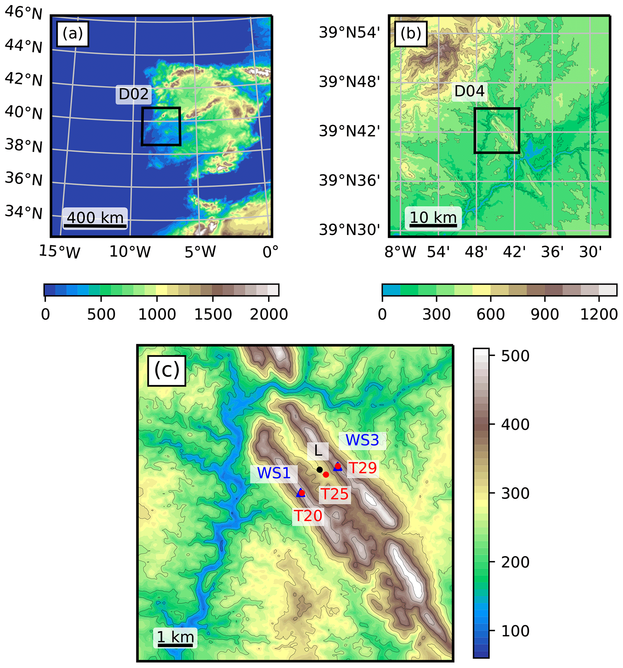
Figure 1 Topographic map of the WRF domains (colour contours). (a) Mesoscale domain D01 using a horizontal grid spacing of 5 km. The extent of D02 is indicated by the black line box. (b) LES Domain D03 using a horizontal grid spacing of 200 m. The extent of D02 is indicated by the black line box. (c) LES Domain D04 using a horizontal grid spacing of 40 m. The locations of the meteorological towers T20, T25 and T29, and the VAD Lidar are marked with dots. The DTU wind scanners WS1 and WS3 are indicated with blue triangles located at the side of towers T20 and T29 (see text for a detailed description). WS2 and WS4 are located at the site of WS1 and WS3, respectively (not shown).

A large amount of instrumentation was deployed in the area near the parallel mountain ridges. The instrumentation included meteorological towers, lidars, microwave radiometers, radiosondes, wind profilers, radio acoustic sounding systems, and microphones providing a unique data pool of meteorological observations in complex terrain (Fernando et al., 2019). In the present work, we use data from the meteorological towers and the lidars to evaluate the numerical model. All the instruments used in the present work are listed in Table 1, and their location is shown in Fig. 1c. Further information on all instrumentation available during the field campaign can be found at the campaign's official web page https://perdigao.fe.up.pt/ (last access: 5 July 2022) (re3data.org, 2019).

Table 1 List of the instrumentation used in the present work along with its location (WSG84 coordinates). The location of each instrument is showed in Fig. 1c.

Data from the 100 m meteorological towers along the southeast transect (TSE; equal to transect 2 in Fernando et al., 2019) are used to evaluate the numerical simulations with and without forest parameterization. The towers were equipped with sonic anemometers at 20, 40 ,60, 80, and 100 m above ground level (a.g.l.).

Four of the wind scanners (WS1–WS4) were performing range-height indicator (RHI) scans across the double ridge parallel to a wind direction of 234.68^∘, which defines TSE. The scanning strategy was such that WS1 and WS3 were scanning towards the southwest using an azimuth angle of 234.68^∘, while WS2 and WS4 were scanning towards the northeast with an azimuth angle of 54.68^∘. Note that WS2 and WS4 are not shown in Fig. 1c, as they are located close to WS1 and WS3, respectively. The combination of the four lidars enables us to produce lidar composites of radial velocities perpendicular to the double ridge (Menke et al., 2019). The latter is called the “cross-valley” direction, and the direction parallel to the double-ridge is called “along-valley” in the present study.

The University of Oklahoma deployed a Halo Photonics Stream Line scanning lidar as part of the Collaborative Lower Atmospheric Mobile Profiling System (CLAMPS, see Wagner et al., 2019c). The instrument was set to different scanning scenarios, but in the present study, we use the data from a regular sequence of velocity azimuth display (VAD) scans every 2 min (see Fig. 1c).

2.2 Numerical simulation setup

The numerical simulations were performed using the WRF model version 4.0.1 (Skamarock et al., 2019). Two sets of LES have been conducted, which differ from each other in the horizontal grid spacing of the innermost domain and the total integration time. The first set consists of long-term simulations ran for 49 d using the same setup as in Wagner et al. (2019a) with three nested domains D01, D02, and D03 with a horizontal grid spacing of 5 km, 1 km and 200 m, respectively (see Fig. 1a and b).

The second set was identical to the first, but it included a fourth nested domain D04 with a horizontal grid spacing of 40 m (see Fig. 1c). The second set, however, was run for selected periods (below described). Domains D01 and D02 were run in RANS (Reynolds Averaged Navier Stokes) mode, while domains D03 and D04 were run in LES mode. The high-resolution of D04 was chosen to better resolve the double ridge. As in Wagner et al. (2019a), vertical nesting was applied to define individual levels in the vertical for each model domain. For the domains D01 to D04, 36, 57, 70, and 82, vertically stretched levels were used, and the respective lowest mass point was set at 80, 50, 15, and 10 m a.g.l.

Previous work has shown that a first model level at 20 m is adequate to represent near-surface flow features in this kind of resolution mesoscale simulations (Quimbayo-Duarte et al., 2021a; Umek et al., 2021).

The model top was set at 200 hPa (about 12 km height). In the RANS domains (D01 and D02), the Mellor–Yamada–Janjic turbulent kinetic energy (TKE) scheme was used (Mellor and Yamada, 1982). In contrast, the simulations in Wagner et al. (2019a) used the YSU scheme (Hong and Kim, 2008). The Eta Similarity (Monin–Obukhov–Janjic) scheme was used to couple the atmosphere and the land surface. The scheme provides the lower boundary conditions for the Level 2.5 model (Janjic, 1996). The Beljaars (1995) correction is applied in order to avoid singularities in the case of free convection and vanishing wind speed (and consequently u). The other physics parameterizations were the same as in Wagner et al. (2019a).

Initial and boundary conditions were provided by the ECMWF operational analyses on 137 model levels with a horizontal grid spacing of 9 km and a temporal resolution of 6 h. The Global 30 Arc-Second Elevation (GTOPO30) digital elevation model and the US Geological Survey (USGS) land use data set were used for D01 and D02, while for D03 and D04, we used the Advanced Spaceborne Thermal Emission and Reflection Radiometer (ASTER) topography data set (Schmugge et al., 2003) with a horizontal grid spacing of 30 m and the Coordination of Information on the Environment (CORINE) land cover data provided in 2012 with a horizontal grid spacing of 100 m. A 10 and 10 min output interval was set for both LES domains (D03 and D04), respectively. To improve the boundary layer flow, a forest parameterization was implemented in the model, which will be described in more detail in the following section.

Both LES were run with the forest parameterization (WRF_d03F, WRF_d04F) and without (WRF_d03NF, WRF_d04NF). Both WRF_d03F and WRF_d03NF were run for 49 d and provided the initial and boundary conditions for the innermost domain simulations WRF_d04F and WRF_d04NF. The high-resolution D04 LES WRF_d04F and WRF_d04NF were run for three selected low-level jet (LLJ) episodes observed during the IOP. Each of the simulations ran for 12 h starting at 18:00 UTC on 6, 7, and 22 May 2017, respectively. From now on, all times will be given in UTC.

2.3 Forest parameterization implementation

The total drag can be modelled by adding the contribution of the orographic pressure (form) drag, the canopy drag, and the (surface) frictional drag. In the standard WRF-LES model, three-dimensional roughness elements like trees are not explicitly considered and are only characterized by the roughness length Z_o (directly obtained from the land use data set), implying that mainly the frictional drag is considered. The explicit treatment of forest drag in numerical models is of special importance for the realistic development of wind profiles, including inflexion points over forested areas.

In the present work, the forest parameterization proposed by Shaw and Schumann (1992) is implemented in the WRF model to study its impact on boundary layer flows over forested and complex terrain. The additional forest drag term F_i (direct sink term in the momentum equation), acting on the lowermost model levels is defined as

$$\begin{array}{}\text{(1)}& F_i=-C_{\mathrm{dLAD}}\left|\mathit{V}\right|u_i,\end{array}$$

where $\left|\mathit{V}\right|$ is the magnitude of the three-dimensional wind vector, u_i is one of the three wind components, C_d=0.15 is a constant drag coefficient, and LAD is the leaf area density profile characterising the trees. The LAD depends on the tree type and the height of the trees, meaning that the strength of F_i varies as one moves in the vertical inside the canopy. The tree type is defined by means of the leaf area index (LAI). Standard similarity expressions hold for the first model level, as the parameterization only introduces a momentum sink; it still needs to couple the atmosphere and the surface. It is worth noting that the momentum is mostly absorbed by the canopy, meaning that the details of the lower boundary condition becomes less important in this case (Ross and Vosper, 2005). The LAD profile is computed according to Lalic and Mihailovic (2004) at all grid cells where trees are present as

$$\begin{array}{}\text{(2)}& \mathrm{LAD}\left(z\right)=L_{\mathrm{m}}{\left({\displaystyle \frac{h-z_{\mathrm{m}}}{h-z}}\right)}^n\exp \left[n\left(\mathrm{1}-{\displaystyle \frac{h-z_{\mathrm{m}}}{h-z}}\right)\right],\end{array}$$

with

$$\begin{array}{}\text{(3)}& n=\left\{\begin{array}{ll}\mathrm{6}& \mathrm{0}\le z<z_{\mathrm{m}}\\ \mathrm{0.5}& z_{\mathrm{m}}\le z\le \end{array}\right.,\end{array}$$

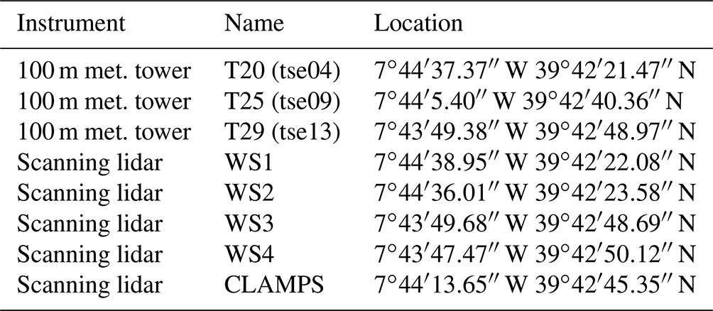
where h is the tree height, and L_m = $(\mathrm{LAI}/h)\cdot \mathrm{1.69}$ is the maximum LAD at height z_m=0.6h following (Mohr et al., 2014). Example LAD-profiles are plotted in Fig. 2 for several LAI using a tree height of 30 m. With increasing LAI, the LAD of the treetop becomes more dominant. The LAI is retrieved from the CORINE land use data set for the present WRF simulations.

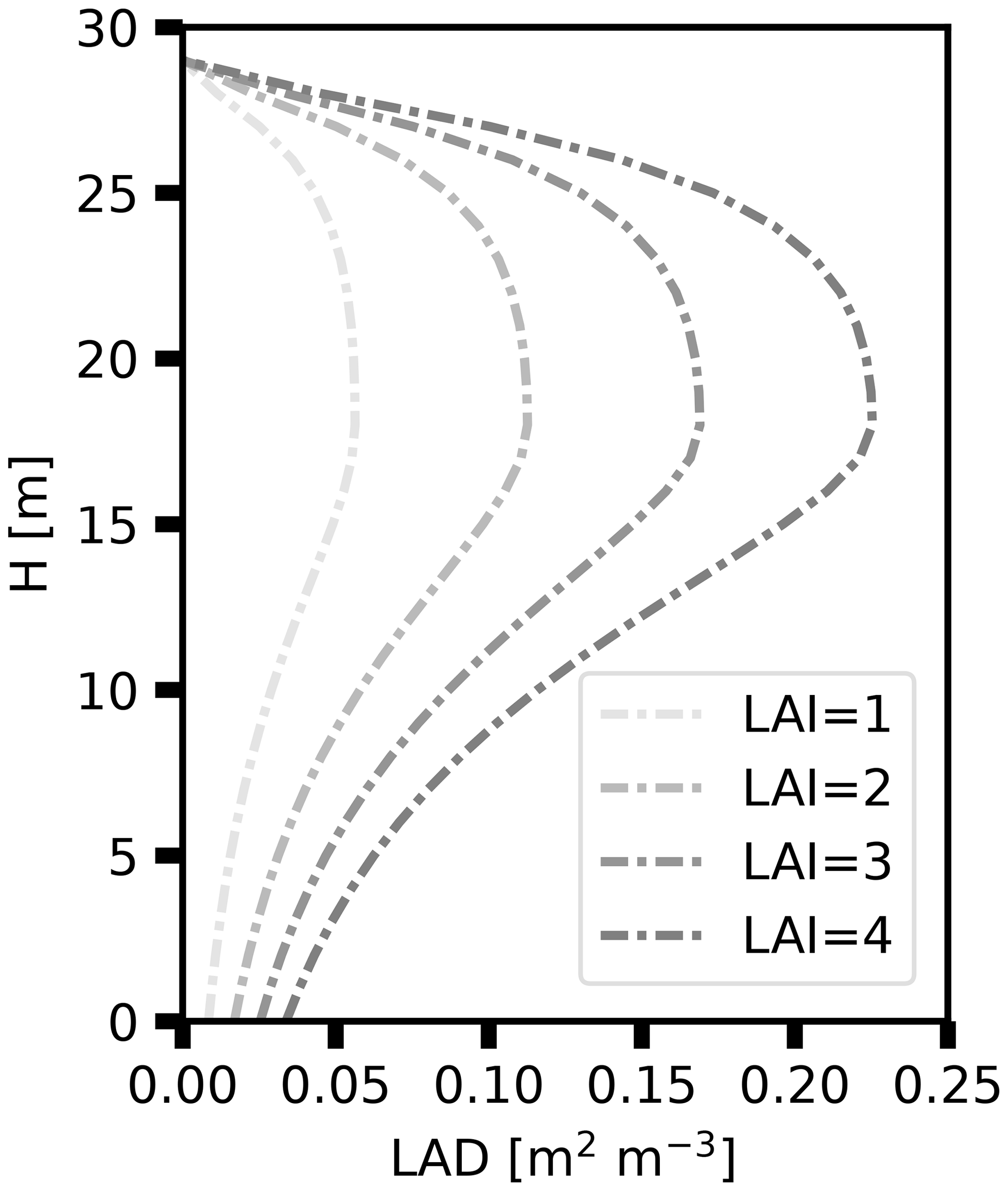
Figure 2 Leaf area density profiles (LAD) for four example values of the leaf area index (LAI) used to parameterize the forest drag. The LAD profiles represent a pine tree canopy.

The LAD profile is computed according to Eq. (1) in regions classified as forest. The forest height is an unknown, as it is not included in the land use data. We used a randomly uniformly distributed tree height of 30±5 m. The tree height used is slightly higher than the trees covering the area, which is about 15–20 m, but it ensures that the lowermost two to three model levels remain within the canopy layer. The profile proposed by Lalic and Mihailovic (2004) is chosen due to its flexibility to represent a broad range of forest canopies by only choosing the appropriated value for the z_m parameter. The Kolic (1978) forest classification, based on z_m and h parameters, lets us divide forest canopies into three groups: (1) z_m=0.2h (oak and silver birch), (2) $\mathrm{0.2}h<z_{\mathrm{m}}<\mathrm{0.4}h$ (common maple), and (3) z_m=0.4h (pine). The parameterization is adaptable for several cases. Following the latter two studies, the empirical relation for the LAD can be applied for a broad range of forest canopies. The site at Perdigão presents an irregular vegetation coverage, made of no or low-height vegetation and patches of eucalyptus and pine trees (Vasiljević et al., 2017). The selection of z_m, consistent with Mohr et al. (2014), is based on the idea of a forest canopy combination between pines and taller eucalyptus threes. We set the LAD to zero in regions not classified as forest. Figure 3a shows the distribution of the LAI for forested regions in the domain D03 as given by the CORINE data set. Figure 3b shows the randomly distributed forest height. White regions mark areas without forest. In the model, the double ridge is completely covered with trees according to the CORINE dataset, which does not fully match the observed forest distribution in the area during the campaign.

Figure 3 Distribution of (a) leaf area index (LAI) and (b) forest height for domain D03. White areas show regions that are not covered by a forest. The topographical height is indicated with contour lines. The extent of D04 is indicated by the black box.

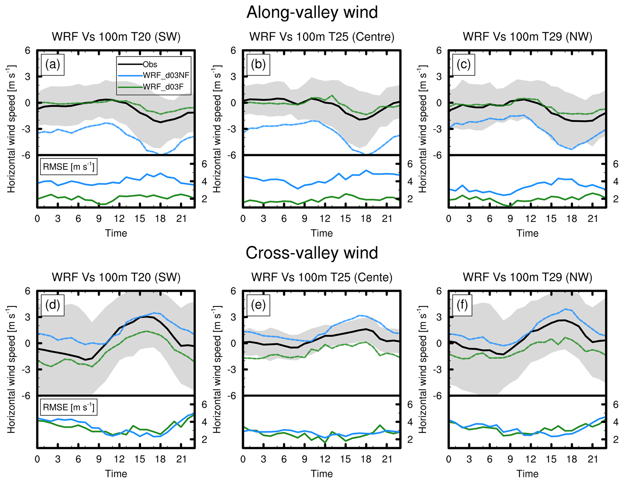
Figure 4 Average diurnal cycle of the along (a–c) and cross-valley (d–f) wind speed for the 49 d IOP for WRF D03 simulation (left axes) (with and without forest parameterization) and the RMSE for the WRF D03 simulations (right axes) at the three tower locations (T20, T25, and T29, see Fig. 1). The black lines represent values for observations (100 m level), the blue lines represent the simulation WRF_d03NF, and the green lines represent the WRF_d03F. The shaded area corresponds to the standard deviation range from observations.

3 Results

In the following, we present an evaluation of the WRF-LES simulations (D03 and D04) with and without the forest parameterization in the context of the Perdigão 2017 field campaign. The analysis is divided into two subsections. First, we evaluate the performance of the long-term simulations (D03). Second, a set of LLJ events is analyzed through the short-term simulations (D04) to investigate the impact of the forest parameterization on the LLJ structure over the double ridge. The analysis and evaluation of the model focus on the performance of the model in simulating the wind field. The simulations showed only small differences in the thermal structure of the atmosphere (not shown).

3.1 Evaluation of the long-term simulations

Figure 4 shows the observed and simulated mean diurnal cycle of both the along and the cross-valley wind speeds averaged over the 49 d period covering the IOP for towers T20, T25, and T29. The root mean square error (RMSE) is shown in the bottom panel for each frame. In the observations, the along-valley wind tends to be very weak in the morning hours. In the afternoon, the wind accelerates to a maximum mean of about 2 m s⁻¹ at 18:00 UTC in all three locations. A significant improvement in the along-valley wind speed is visible when the forest parameterization is used (WRF_d03F). At all three towers, the RMSE is typically less than half of its original value for the simulation without the forest parameterization (WRF_d03NF).

In the cross-valley direction, the wind observed in the early morning is weak at all three locations. At around 18:00 UTC, at the crest towers (T20 and T29), the mean cross-valley wind speed reaches its maximum at about 3 m s⁻¹. In the valley bottom, the maximum wind speed reaches out about 1.5 m s⁻¹. After the evening transition, the flow slows down, and at midnight it is nearly zero. As noted by Wagner et al. (2019a), the observations showed the presence of a clear daily cycle due to the dominant synoptically calm conditions enhancing the evolution of thermally driven flow systems during the second part of the IOP.

The cross-valley wind speed in the WRF_d03NF simulation is overestimated throughout the day (see Fig. 4d–f). The introduction of the forest parameterization in the WRF_d03F simulation addresses this problem. However, the effect is too strong, and the wind speed is underestimated at all three towers. In terms of the RMSE, there is no significant difference between the two simulations. Both simulations remain in the range of the standard deviation of observations (shaded areas).

Figure 5 As in Fig. 4 but for the diurnal cycle of the vector-averaged wind direction.

Figure 5 shows the mean diurnal cycle of the wind direction, vector-averaged through the 49 d simulation (and observations) covering the IOP for towers T20, T25, and T29. It is important to note that this is a cyclic measure, both top and bottom ends of the figures represent wind coming from the north. In both crest towers, the wind blows from the northeast in the morning hours. Around noon, it changes the direction to become northwest at the end of the day. In the valley, tower (T25), the flow is channelled in the up-valley direction (southeast) through the early morning until 08:00 UTC. In the following hours, the wind slowly turns to become down-valley (northwest) in the afternoon until late at night (about 22:00 UTC).

In the WRF_d03NF simulation, the model cannot accurately represent the wind direction in the morning hours. The flow is always northwesterly throughout the day. This issue is corrected in the WRF_d03F simulation, where the flow follows the trend in the observations during the morning and afternoon hours at all three towers.

The underestimation of the wind speed in the cross-valley direction in WRF_d03F simulation may indicate that the use of tree heights of 30±5 m is too high, and an improvement in the land use data with a more realistic LAI and forest height distribution is necessary. Menke et al. (2020) used data from two pairs of scanning lidars operated in a dual-Doppler mode during the Perdigão 2017 field campaign to evaluate the performance of WRF-LES along the ridges (using a similar configuration to WRF_d03F). Their results evidence a high sensitivity to the parameterization of surface friction. The model fails to reproduce the correct signal for the wind amplitude along the ridges both with and without the forest parameterization, although an improvement in the results is observed for the simulation using the forest parameterization. The authors suggested that the model performance can be improved with a more realistic description of the horizontal distribution of forested areas and tree heights in the numerical domain.

3.2 Evaluation short-term simulations

LLJ events, which are mostly a night-time phenomena, are frequently observed above the double ridge. During the IOP, LLJs are mainly the product of thermally driven flows generated by the surrounding mountainous area under synoptically calm atmospheric conditions. Jets from the northeast occurred more frequently than jets from the southwest (Wagner et al., 2019a).

Short-term, high-resolution numerical simulations with the forest parameterization (WRF_d04F) and without (WRF_d04NF) are evaluated for three LLJ events observed during the IOP and highlighted in Wagner et al. (2019a). Northeast LLJ events during the nights of 7 and 8 May 2017 and a southwest LLJ event on the night of 22 May 2017 were selected to be analyzed in the present work. These events were selected, as the jets observed are very stationary.

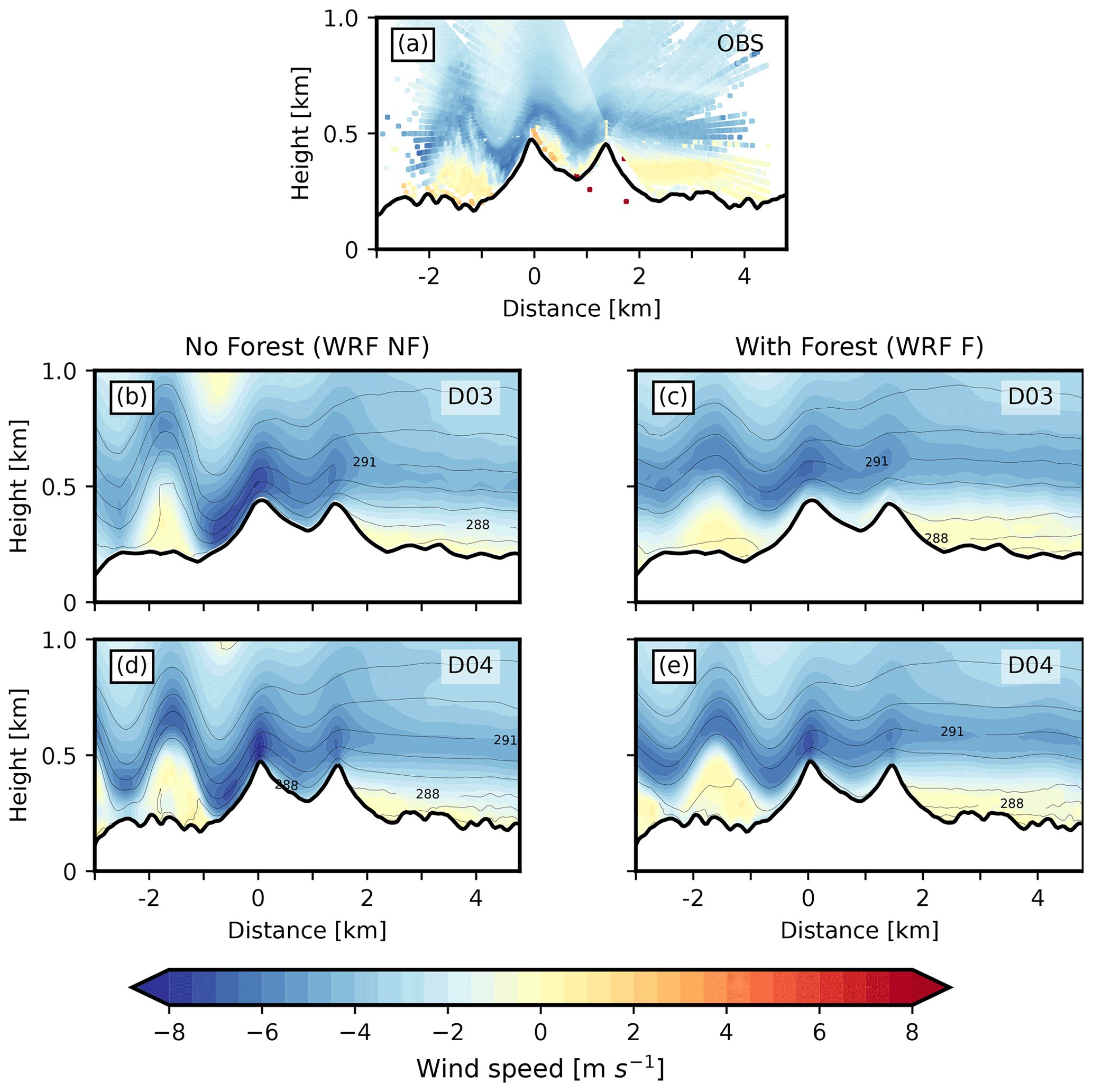
Figure 6 Cross-sections of cross-valley wind speed (horizontal wind component across the double ridge) for the low-level jet (LLJ) event from NE on 7 May 2017 at 04:00 UTC. The x-axis is centred at the location of WS1. Negative velocities indicate flow from NE. (a) Observed winds retrieved from radial velocity composite of DTU Lidars WS1 to WS4. Colour contour interval: 0.5 m s⁻¹. The topography illustrated is identical to that used for D04. (b–e) Simulated winds and potential temperature from WRF numerical model. Model data was interpolated to the same cross-section as for the observations, which was defined by the location of WS1 and the azimuth scanning angle of 234.68^∘. WRF simulations without the forest parameterization are displayed in left column, simulations using the forest parameterization are displayed in the right column, for domain D03 (b–c) and D04 (d–e).

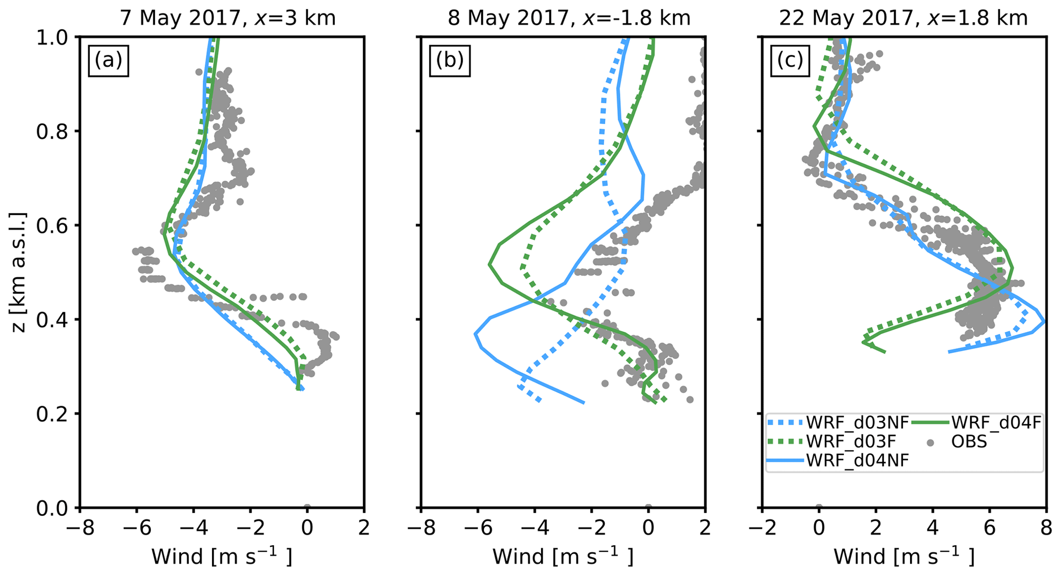
Figure 7 Vertical profiles of the wind speed parallel to the cross-sections (see Figs. 6, 8, and 9) during the low-level Jet (LLJ) events for both simulations (colour lines) and lidar observations (grey dots). Panel (a) presents the first LLJ event (7 May 2017 04:00:00 UTC) on the leeward side of the topography (x=3 km). Panel (b) presents the second LLJ event (08 May 2017 05:30:00 ) on the leeward side of the topography ($x=-\mathrm{1.8}$ km). Panel (c) presents the third LLJ event (22 May 2017 04:00:00 UTC) on the leeward side of the topography (x=1.8 km).

Figure 8 As in Fig. 6 but for the low-level jet case on 8 May 2017 05:30:00 UTC.

Figure 9 As in Fig. 6 but for low-level jet case on 22 May 2017 04:00:00 UTC.

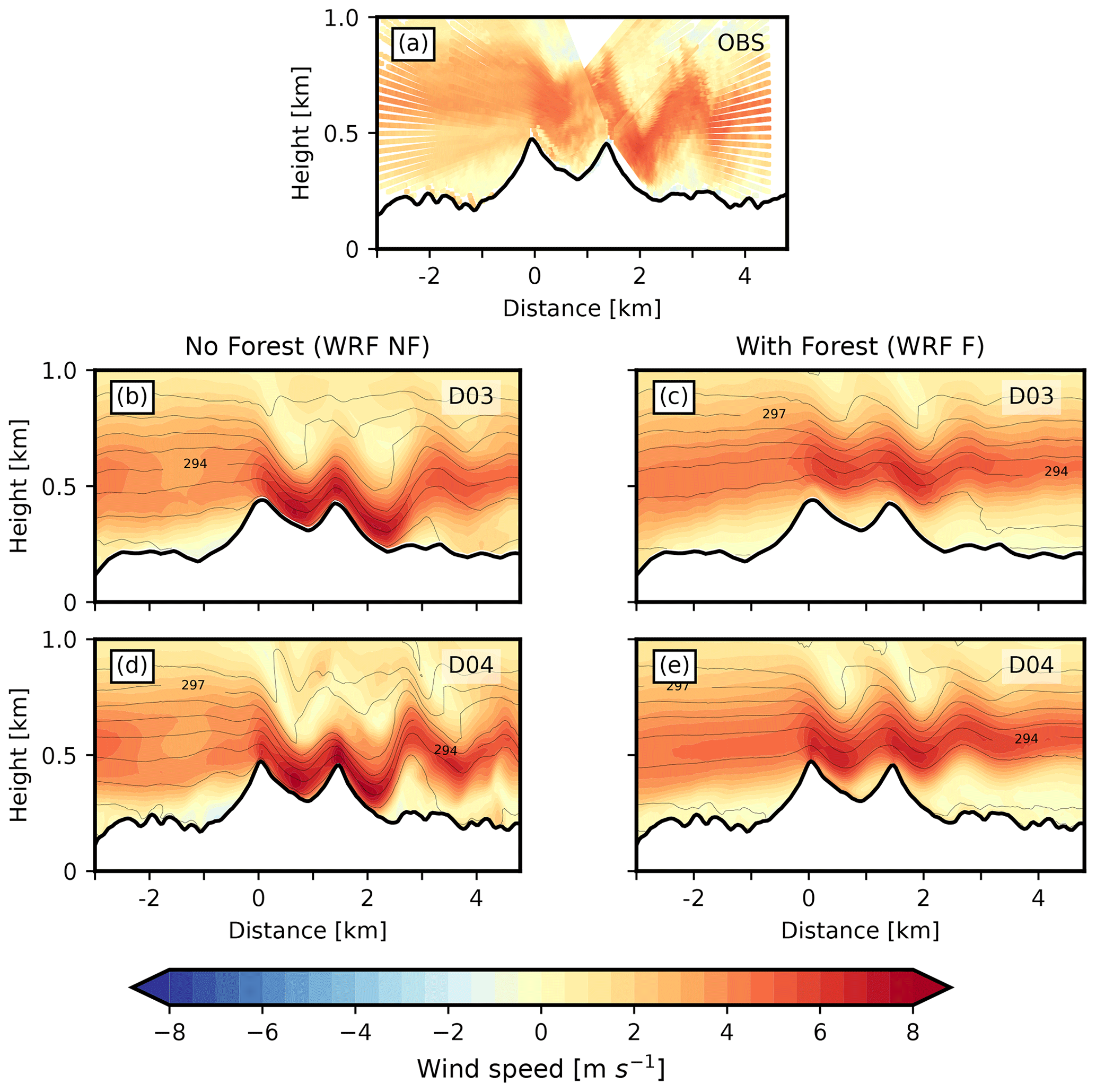
Panel (a) in Figs. 6, 8, and 9 shows lidar composites of the four DTU wind scanners WS1 to S4 to represent the valley cross-section horizontal wind structure. Panels (b) to (e) show snapshots of the cross-valley wind speed (colour contours) and potential temperature of simulations using the forest parameterization (WRF_d03F and WRF_d04F) and without (WRF_d03NF and WRF_d04NF) for the same time as the respective observed cross-valley winds.

The LLJ event on the early morning of 7 May is observed in the lidar composite (see Fig. 6a). The flow comes from the northeast with strong wind speeds (about 5 m s⁻¹) close to the topography (starting at about 0.5 km a.s.l.) and easterly winds above. In the leeward side of the topography, the signature of internal gravity waves is observed ($-\mathrm{2.5}<x<\mathrm{0}$ km). The horizontal wavelength is similar to that of the valley (about 1.4 km).

Both WRF_d03NF and WRF_d04NF capture the main features of the LLJ episode. The LLJ and the internal gravity wave structure on the leeward side of the topography (for $-\mathrm{4}<x<\mathrm{0}$ km) can be observed in the snapshots of both simulations without using the forest parameterization. However, WRF_d03NF and WRF_d04NF cannot represent the observed southwest flow near the ground, between the surface and 0.25 km a.s.l., on the leeward side of the topography (positive wind in Fig. 6). This feature is better observed in Fig. 7a, where vertical profiles for wind speed for both simulations and observations are displayed at x=3 km. The observations show a weak wind above the surface followed by a positive wind of about 1 m s⁻¹ up to 0.4 km a.s.l. The simulations without the forest parameterization (blue lines in Fig. 7) fail to capture such a feature. On the other hand, simulations using the forest parameterization (green lines in Fig. 7) capture the quiet wind close to the ground and compare better with observations in the first 0.5 km a.s.l.

On the leeward side, the wave amplitude is too large (wave crest up to 1 km a.s.l.) in simulations WRF_d03NF and WRF_d04NF when compared with observations where the wave crest only reaches 0.75 km a.s.l. Simulations using the forest parameterization better represent the wave structure, especially WRF_d04F, where the simulations nicely capture the wave structure (for $-\mathrm{2.5}<x<-\mathrm{1.5}$ km) for both wave length (about 1.4 km) and wave amplitude (0.5 km).

On the following day (8 May), another northeasterly LLJ event was observed, but with a southwesterly upper-level wind (see the orange colours above 0.7 km a.s.l.). The signature of orographically induced gravity waves is visible in the lidar observations near the topography in Fig. 8a. All simulations fail to simulate the southwesterly upper-level wind, which seems to be related to large-scale phenomena coming from the boundary conditions driving the model. The simulations using the forest parameterization better capture the near the surface atmosphere by reproducing the LLJ and the southwesterly wind between the ground and the LLJ (see Fig. 8c and e). Simulations without the forest parameterization show a deep LLJ reaching down to the ground on the lee side of the topography, which is not observed in the lidar data. Figure 7b details the wind structure on the leeward side at $x=-\mathrm{1.8}$ km. Simulations without the forest parameterization show an erroneous negative wind (which may be very strong up to 6 m s⁻¹) close to the surface. On the other hand, simulations using the forest parameterization compare well with the observations near the ground up to 0.4 km a.s.l., especially WRF_d04F.

The third LLJ event occurred in the early morning of 22 May (see Fig. 9). The event corresponds to a southwesterly LLJ. The LLJ layer is deeper (about 700 m deep) when compared to the other two episodes. Again, the signature of gravity waves is observed in the lidar data on the leeward side of the topography. In this event, all simulations reproduce the main features of the LLJ. The wind direction and magnitude seems to be appropriate in all simulations. However, the forest parameterization in WRF_d04F seems to prevent the LLJ from flowing along the leeward slope as observed in the lidar data. Figure 7c details the wind structure at the mid-leeward slope (x=1.8 km). The simulations without the forest parameterization fit better with observations in the first metres above the ground by representing a positive strong wind reaching about 6 m s⁻¹ as observed in the lidar data. Simulations using the forest parameterization worked especially well above 200 m a.s.l., where both lines (green lines) fit well with the observations. However, close to the surface, the simulations using the forest parameterization underestimate the flow where only a weak flow (less than 2 m s⁻¹) is simulated. In this case, it seems that the forest parameterization works better when the flow is from the northeast rather than from the southwest. The latter can be explained by the fact that at the northeast facing slope of the downwind ridge, the tree population is not well described in the model (which, in reality, is mainly covered by low vegetation), resulting in higher drag, which accounts for the lower wind speed simulated.

In general, the jet structure and the flow close to the surface agree better with lidar observations when the forest parameterization is switched on (with the exception of the last event in the lee slope). Surface winds are reduced, recirculation zones develop, and the amplitudes of the gravity waves agree better with lidar observations. A better representation of the surface friction has a significant impact on the formation and wavelength of trapped lee waves (Stiperski and Grubišić, 2011).

Up to this stage, the evaluation of the high-resolution LES was carried out for single time snaps to capture the main features of the atmosphere in a cross-valley section. In the following, the model performance is evaluated for the period between 7 and 8 May, which comprises the first two LLJ events at a single tower location (T25).

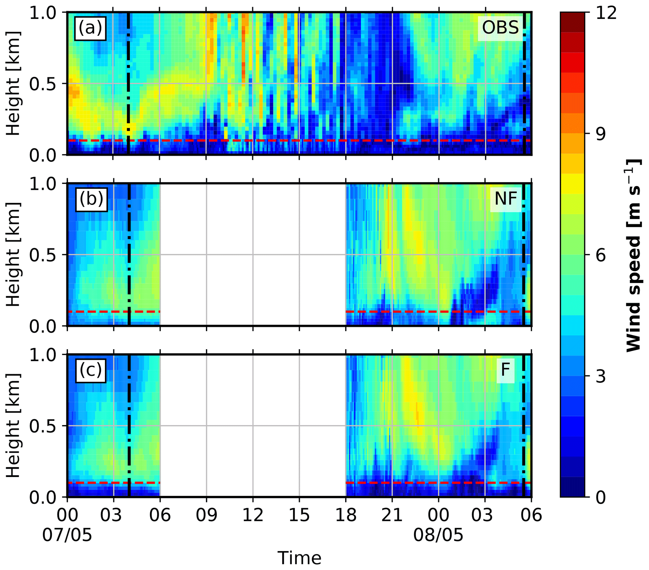
Figure 10 Vertical and temporal structure of the horizontal wind speed from observations using data from the tower T25 up to 100 m, and the University of Oklahoma's VAD wind profiling scans from 100 up to 1000 m (a). Simulation without the forest parameterization (WRF_d04NF) (b) and with the forest parameterization (WRF_d04F) (c). The results for the WRF simulations have been taken at the nearest grid point to the location where the University of Oklahoma's wind profiler scan was located during the field campaign (see Fig. 1c). Dashed red lines in the plots represent the 100 m above ground height. The vertical dash-dotted black line represents the time at which LLJ events were observed (see text for reference).

Figure 10 shows the temporal evolution of the wind speed vertical profiles at the valley centre between 00:00 UTC on 7 May and 06:00 UTC on 8 May for both the observations and the numerical simulations. Figure 10a presents the data from the tower T25 (20–100 m a.g.l.) and the VAD wind profiling scans (100–1000 m a.g.l.). The instruments are located 250 m from each other. During the early hours of 7 May (00:00–06:00 UTC), the lower atmosphere is characterized by a 100 m deep weak flow layer (below 3 m s⁻¹; see the dark blue colours near the surface in Fig. 10a). The LLJ signature is observed aloft (between 150 and 400 m a.g.l.) reaching wind speeds of about 8 m s⁻¹ between 02:00 and 06:00 UTC. After 06:00 UTC, the near-surface layer of weak wind increases to a depth of over 200 m at 09:00 UTC. During midday and afternoon (11:00–18:00 UTC), the whole layer becomes turbulent, and a convective signal is observed until 18:00 UTC when turbulence begins to vanish and the nocturnal stable boundary layer dominates after 22 h.

In the early hours of 8 May (00:00–03:00 UTC) the LLJ is hardly visible. The weak flow layer close to the ground is deeper than the day before (as deep as 200 m), and the wind close to the surface remains weak. At 03:00 UTC, the flow layer starts to deepen, reaching 500 m at 6:00 UTC while maintaining the magnitude of the wind speed.

Panels (b) and (c) in Fig. 10 present the results for WRF_d04NF and WRF_d04F, respectively, at the location of the tower T25. Both simulations ran for 12 h between 18:00 and 06:00 UTC for 6 and 7 May, respectively. The simulations capture the main features observed in the tower and the lidar data. However, important differences can be noted. The LLJ event observed in the early morning of 7 May (00:00–06:00 UTC) is reproduced by both simulations, but is weaker than observed. WRF_d04NF fails to correctly reproduce the layer of weak flow close to the ground (shallower than observations, about 50 m deep). This issue is addressed by WRF_d04F. The introduction of the forest parameterization helps in slowing down the flow close to the ground. This thus improves the representation of the near-surface winds by creating a deeper flow layer (100 m) between 00:00 and 06:00 UTC (see Fig. 10c), which is not represented in WRF_d04NF (see Fig. 10b).

In the second simulation period (18:00 UTC 7 May–06:00 UTC 8 May), both simulations overestimate the magnitude of the LLJ between 18:00 UTC and midnight by showing wind speeds as high as 8 m s⁻¹, while the observations showed a quiet wind barely reaching 3 m s⁻¹.

WRF_d04NF better represents the near-surface flow layer (200 m deep) than the previous night (00:00–06:00 UTC 7 May). Again, WRF_d04F captures the weak character of such a layer better. WRF_d04F simulated the 200 m deep flow layer above the ground between 18:00 UTC and midnight well, showing a weak 1 m s⁻¹ flow as evidenced in the observations. At about 02:00 UTC, the atmosphere becomes quiet and the ground flow layer linearly grows reaching 600 m at 05:00 UTC in both simulations and observations.

To quantify the impact of the forest parameterization on the wind profile, the RMSE, the bias and the average wind speed are calculated at the T25 tower location. The calculation is based on the two simulated periods; between 00:00 to 06:00 UTC 7 May (Fig. 11a–c) and 7 May at 18:00 UTC to 8 May at 06:00 UTC (Fig. 11d–f). Figure 11 shows the results for both WRF_d04NF and WRF_d04F simulations.

Figure 11 Vertical profiles of the root-mean-squared error (RMSE, a and d), bias (b and e), averaged vertical profiles of the of wind speed (c and f) for WRF_d04NF (blue lines), and WRF_d04F (green lines). The observations of the wind speed in panel (c) and (f) are displayed with the black line. From the ground up to 100 m, data from the tower T25 is used, while from 100 to 1000 m data from the University of Oklahoma's VAD wind profiling scans is used. The dashed grey line marks the 100 m level. The results were computed between 7 May 00:00–06:00 UTC (a, b, and c) and 7 May 18:00 UTC–8 May 06:00 UTC (d, e,and f).

The influence of the forest parameterization in the first 100 m a.g.l. is important for both simulated periods. The WRF_d04F performance is consistently better than WRF_d04NF, having the largest difference near the surface, where WRF_d04F presents 1.5 and 1 m s⁻¹ difference to WRF_d04NF in terms of the RMSE (see Fig. 11a and d) for the first and second periods, respectively. The effect of the parameterization vanishes with height; however, its effect can be observed up to 500 m a.g.l., especially during the second period.

A similar behaviour is found For the bias (see Fig. 11b and e). WRF_d04F improves the model performance for the first few hundreds metres above the ground. It is worth noting that both simulations overestimate the wind speed through the first 100 m a.g.l. The forest parameterization adds drag, which helps to slow down the near-surface wind, leading to smaller error. The latter is well summarized in Fig. 11c and f, where the average vertical profiles of the wind speed show the overestimation of the wind speed close to the ground (up to 200 m a.g.l.) in both simulations. However, the simulation using the forest parameterization fits the observations better in the first 150 m a.g.l. for the first period, and 400 m a.g.l. above the ground for the second period, improving the model performance. The effect of the forest parameterization evolve as the atmospheric conditions vary. For the first period, the effect it is as deep as 150 m a.g.l., while it is three times deeper for the second period.

Above 100 m a.g.l. both WRF_d04F and WRF_d04NF simulations tend to underestimate the wind speed maxima (see Fig. 11c). This may be a consequence of a misrepresentation of the thermally driven flow in the Serra da Estrela mountain range (NE of Perdigão) in the NWP simulation driving both high-resolution simulations. The latter negatively impacted the reproduction of the wind flow during the night hours at the Perdigão site.

Figure 12 As in Fig. 10, but for the wind direction.

Figure 12 shows the temporal evolution of the wind direction at the tower T25 location for both the observations and the numerical simulations. Observations show an upper level wind from the southeast throughout the whole period. The LLJ event observed in the early morning of 7 May 00:00 to 06:00 UTC corresponds to a northeasterly cross-valley wind. Near the ground (below 100 m a.g.l.), a wind from the north/northeast dominates (cross-valley). During the day hours (06:00 to 18:00 UTC), the up-valley wind (southeast) dominates the convective atmosphere with some turbulent burst of north/south winds. During the following night, the up-valley wind (southeast) near the ground (below 80 m a.g.l.) does not change direction and remains up-valley until the end of the simulated period at 06:00 UTC. Immediately above the ground flow layer (between 100 and 300 m a.g.l.), a cross-valley wind (northeast) is observed, which may be interpreted as the signature of the LLJ.

Both WRF_d04NF and WRF_d04F simulations capture the main features of the flow. A northeasterly wind is simulated at 100 m a.g.l. between 00:00 and 06:00 UTC 7 May. However, during this period both simulations failed to capture the southeasterly flow above 200 m a.g.l. Instead, a northeasterly wind was simulated. A constant up-valley wind near the ground was observed through out the period, which is not represented in the WRF_d04NF simulation and only partially simulated for some short periods of time (see, for instance, 8 May between 20:00 and 22:00 UTC) in WRF_d04F. During the second night (8 May), both simulations captured the southeasterly wind observed above 200 m a.g.l. between 21:00 and 06:00 UTC.

It is worth noting that the wind speed near the surface is very weak (below 3 m s⁻¹), which makes the task to capture the proper wind direction challenging. Above the near-surface flow layer, where the wind is stronger, the model displays a better performance. Since at low wind speeds, wind direction fluctuations are important, statistics of this quantity have not been calculated due to the possible large RMSE values that may lead to misinterpretation of the results (Chow et al., 2006).

4 Conclusions

The performance of high-resolution mesoscale simulations using the Weather Research and Forecasting (WRF-V4.0.1) model (Skamarock et al., 2019) with and without the implementation of a forest parameterization has been tested in the context of the Perdigão 2017 field campaign (Fernando et al., 2019). A similar configuration to that presented in Wagner et al. (2019a) is used with the addition of a subsequent inner domain with a horizontal grid spacing of 40 m. Results are validated and tested against observational data retrieved during the campaign's intensive observational period (IOP) between April and June 2017.

Long-term simulations (49 d) covering the IOP were conducted using a horizontal grid spacing of 200 m. The mean diurnal cycle during the IOP shows a significant improvement of the along-valley wind speed and wind direction when using the forest parameterization (WRF_d03F). However, the drag imposed by the parameterization results in an underestimation of the cross-valley wind speed. This may indicate that the specified tree height of 30±5 m is too high, and an improvement in the land use data with a more realistic leaf area index (LAI) and forest height distribution is necessary.

Low-level jets (LLJ) events, which are mostly night-time phenomena, are frequently observed above the double ridge (Wagner et al., 2019a). Short-term, high-resolution numerical simulations, using a 40 m horizontal grid spacing, with the forest parameterization (WRF_d04F) and without (WRF_d04NF) are evaluated for three LLJ events observed during the IOP.

The simulations using the forest parameterization capture the main features of the observed LLJ better than the simulations without it. The additional drag from the forest parameterization helps to better reproduce the near-surface flow structure with re-circulation zones near the slopes that agree better with the lidar observations.

The model performance is further evaluated for the period comprising the first two LLJ events for the valley tower site (T25). The forest parameterization systematically improves the representation of the wind near the surface, both the wind magnitude and the wind direction, throughout the LLJ events. Although the parameterization is only applied to the first three model levels (about 30 m a.g.l.), its positive impact is visible up to a height of 500 m a.g.l., in terms of a reduced RMSE and bias.

In general, the simulations using the forest parameterization capture the main features of the observed LLJ better than the simulations without it. The additional drag from the forest parameterization helps to better reproduce the near-surface flow structure with the observed re-circulation zones near the slopes. A representation of the forest as a roughness element with an increased value of z₀ seems to be inappropriate in these high-resolution mesoscale simulations. The addition of a forest parameterization can positively influence the simulation of the winds in the boundary layer over moderately complex terrain.

Further improvement might be achieved with the use of more accurate land use data with a more realistic LAI and forest height distribution. The investigation of the benefit of a forest parameterization for other atmospheric conditions and different locations is left for future work.