An aerosol classification scheme for global simulations using the K-means machine learning method

The K-means machine learning algorithm is applied to climatological data of seven aerosol properties from a global aerosol simulation using EMAC-MADE3. The aim is to partition the aerosol properties across the global atmosphere in specific aerosol regimes; this is done mainly for evaluation purposes. K-means is an unsupervised machine learning method with the advantage that an a priori definition of the aerosol classes is not required. Using K-means, we are able to quantitatively define global aerosol regimes, so-called aerosol clusters, and explain their internal properties and their location and extension. This analysis shows that aerosol regimes in the lower troposphere are strongly influenced by emissions. Key drivers of the clusters' internal properties and spatial distribution are, for instance, pollutants from biomass burning and biogenic sources, mineral dust, anthropogenic pollution, and corresponding mixtures. Several continental clusters propagate into oceanic regions as a result of long-range transport of air masses. The identified oceanic regimes show a higher degree of pollution in the Northern Hemisphere than over the southern oceans. With increasing altitude, the aerosol regimes propagate from emission-induced clusters in the lower troposphere to roughly zonally distributed regimes in the middle troposphere and in the tropopause region. Notably, three polluted clusters identified over Africa, India, and eastern China cover the whole atmospheric column from the lower troposphere to the tropopause region. The results of this analysis need to be interpreted taking the limitations and strengths of global aerosol models into consideration. On the one hand, global aerosol simulations cannot estimate small-scale and localized processes due to the coarse resolution. On the other hand, they capture the spatial pattern of aerosol properties on the global scale, implying that the clustering results could provide useful insights for aerosol research. To estimate the uncertainties inherent in the applied clustering method, two sensitivity tests have been conducted (i) to investigate how various data scaling procedures could affect the K-means classification and (ii) to compare K-means with another unsupervised classification algorithm (HAC, i.e. hierarchical agglomerative clustering). The results show that the standardization based on sample mean and standard deviation is the most appropriate standardization method for this study, as it keeps the underlying distribution of the raw data set and retains the information of outliers. The two clustering algorithms provide similar classification results, supporting the robustness of our conclusions. The classification procedures presented in this study have a markedly wide application potential for future model-based aerosol studies.

1 Introduction

Aerosols play an important role in the climate system (Boucher et al., 2013). They influence climate directly via scattering and absorption of solar and terrestrial radiation and indirectly via modifications of cloud properties. The major components of atmospheric aerosols are mineral dust, black carbon (BC), organic carbon, sulfate, nitrate, ammonium, and sea salt. Due to their relatively short residence times, the contributions of these components, their state of mixing, and the particle size distribution show a large spatial and temporal variability on the global scale (e.g. Lauer and Hendricks, 2006; Mann et al., 2010, 2014; Pringle et al., 2010; Aquila et al., 2011; Sessions et al., 2015; Kaiser et al., 2019). Additionally, their effects on clouds and radiation are highly variable due to the strong dependencies on the physical and chemical properties of the aerosols. This in combination with uncertainties in the current knowledge of key aerosol-related processes makes the quantification of aerosol–climate effects a challenge and results in comparatively large uncertainties in the existing quantifications of the climate impact of anthropogenic aerosols (e.g. Boucher et al., 2013; Myhre et al., 2017; Bellouin et al., 2020).

Global aerosol–climate models equipped with detailed representations of aerosol microphysical and chemical processes are essential tools for the quantification of aerosol–climate effects (e.g. Boucher et al., 1998; Takemura et al., 2005; Stier et al., 2005, 2006; Lauer et al., 2007; Hoose et al., 2008; Righi et al., 2013, 2020; Randles et al., 2013; Kipling et al., 2016; Myhre et al., 2017; Bellouin et al., 2020). During the last few decades, considerable attempts have been made by the global aerosol modelling community to develop improved descriptions of aerosol–climate interactions (e.g. Ghan and Schwartz, 2007; Boucher et al., 2013; Riemer et al., 2019). Early modelling approaches considered only the mass of aerosol species. However, observations imply that the number, size distribution, and mixing state of aerosols are also critical factors for an accurate representation of aerosol–climate interactions (Albrecht et al., 1989). The first attempts at representing the aerosol size distribution and mixing state in global models started at the end of the 20th century (e.g. Jacobson, 2001). Due to limited computing capacities and the huge computational expenses of global aerosol–climate models, cost-effective algorithms have been applied, for instance, the lognormal representations of the aerosol size distribution (e.g. Stier et al., 2005; Lauer et al., 2006; Aquila et al., 2011; von Salzen, 2006; Pringle et al., 2010; Kaiser et al., 2019). Recent approaches allow for tracking soluble and insoluble aerosol particle components, as well as their mixtures, and facilitate the simulation of particle number, mass concentration, and size distribution. Beyond the direct radiative impact of aerosols, aerosol–cloud interactions are key processes driving aerosol–climate effects. Hence, parameterizations of aerosol activation in liquid clouds have been established (see Ghan et al., 2011, for a review). In addition, aerosol-induced formation of ice crystals has attracted increasing attention (Kanji et al., 2017; Heymsfield et al., 2017). To represent the manifold ice formation pathways induced by a large number of different aerosol types in global aerosol–climate models, the applied microphysical cloud schemes, as well as the underlying aerosol sub-models, have been further extended (e.g. Lohmann and Kärcher, 2002; Kärcher et al., 2006; Lohmann et al., 2007; Lohmann and Hoose, 2009; Hendricks et al., 2011; Kuebbeler et al., 2014; Righi et al., 2020).

The above examples demonstrate the growing complexity of global aerosol models, which consequently results in a large number of parameters that describe the aerosol number concentration, size distribution, and composition and makes the analysis, evaluation, and interpretation of the model results a challenge. This is further complicated by the large spatial and temporal variability of the aerosol properties. Under these circumstances, analysing all relevant variables from a typical global model simulation can become unfeasible. New analysis methods are therefore required to gather information from the huge set of variables and their temporal and spatial variability. A powerful tool to facilitate the analysis of global aerosol model results is the partitioning of the model-simulated aerosol into different groups or clusters, each characterized by specific properties. In the following, these groups will be called aerosol regimes. Information about how these aerosol regimes are distributed in space could be very helpful to obtain a concise but comprehensive view of the complex system of modelled aerosol parameters. Detailed knowledge of the spatial distribution of individual aerosol regimes could be the basis for further analyses and model improvement. For instance, observations within a specific aerosol regime can be combined for evaluating simulation results with regard to this specific aerosol type. Furthermore, model evaluation results based on observations limited in space and time (e.g. aircraft-based field campaigns), could be generalized to a whole aerosol regime covering much larger areas and time periods, assuming that the systematic model biases to be corrected occur nearly homogenously throughout the whole cluster. In addition, knowledge of the properties and spatial extension of aerosol regimes could serve as supportive information for satellite retrieval and for the planning of further field campaigns for aerosol observation.

Previous aerosol classifications have been mainly conducted in the context of observational studies using measurements of aerosol microphysical and optical properties. For example, Groß et al. (2013, 2015) applied classification schemes to identify specific aerosol types and their mixtures based on lidar measurements and satellite data. Their classification procedure follows a tree structure where different aerosol microphysical and optical properties imply different classification branches. This allows the identification of complicated vertical stratifications of different aerosol types throughout the atmosphere. Bibi et al. (2016) applied multiple clustering techniques to analyse seasonal differences in prevailing aerosol types at four locations in India. Their classification was based on the analysis of pairs of aerosol optical properties gained from the Aerosol Robotic Network (AERONET) sun photometer measurements. Schmeisser et al. (2017) applied a similar multiple clustering technique to classify aerosol types based on surface-based observations of spectral aerosol optical properties from a global station network. Nicolae et al. (2018) classified six aerosol types using an artificial neural network applied to lidar measurements. The neural network was trained with predefined data from different aerosol types. Applying similar algorithms to global model results using optical aerosol properties to classify aerosol types, however, could be problematic since the optical properties are derived quantities that are calculated from primary (prognostic) quantities such as aerosol number, size, and composition. These calculations also require additional assumptions, usually retrieved from measurements of, e.g. aerosol refractive indices, possibly implying further uncertainties (Dietmüller et al., 2016). Hence, new algorithms for aerosol classification based on primary aerosol model parameters would be more appropriate.

In this study, we apply the K-means machine learning clustering algorithm (Hartigan and Wong, 1979) for identifying clusters of specific aerosol types in global aerosol simulations. This method partitions n samples into k clusters in which each sample is assigned to the cluster with the nearest distance to the clusters' centre (or cluster centroid). K-means is classified as an unsupervised machine learning algorithm. This is especially useful when the classification criteria are unknown, as in the case of aerosol classification where the specific aerosol characteristics for the predominant regimes are not known a priori. In comparison with supervised classification algorithms, which require substantial prior knowledge of classes, an unsupervised classification is relatively easy to use, but it requires the identification and labelling of the resulting clusters after the classification. The common known limitations of K-means include the presence of clusters with equal variances and its sensitivity to outliers. K-means has already been applied in atmospheric research. For instance, it has been successfully used to distinguish clouds and aerosols in CALIOP/CALIPSO observations (Zeng et al., 2019). In this study, we apply the K-means algorithm to global aerosol simulations. The main goal is to answer the following questions: (1) how can major aerosol regimes be identified in global aerosol simulations, (2) what is the spatial distribution of these regimes, and (3) which aerosol types are dominant in which parts of the world? The K-means method is applied here to identify clusters of different aerosol types in global simulations. The spatial extension of these clusters is quantified. The aerosol properties considered for the clustering process were simulated using the global chemistry–climate model system EMAC (the ECHAM/MESSy Atmospheric Chemistry general circulation model, Jöckel et al., 2010, 2016) equipped with the aerosol microphysical sub-model MADE3 (Modal Aerosol Dynamics model for Europe adapted for global applications, third generation, Kaiser et al., 2014, 2019). The aerosol properties analysed here include the mass concentrations of mineral dust; BC; particulate organic matter (POM); sea salt; the sum of aerosol sulfate, nitrate, and ammonium (SNA); and particle number concentrations in different aerosol size modes. The clustering analysis is conducted separately for the lower troposphere, the middle troposphere, and the tropopause region. To quantify potential uncertainties of the clustering procedure, the sensitivity of the results to different methods for scaling the input data is explored. We also provide a comparison of K-means clustering with another unsupervised machine learning clustering algorithm, namely hierarchical agglomerative clustering (HAC).

The paper is structured as follows. Section 2 describes the model data and the analysis methods in detail. The results of the global clustering procedure are presented in Sect. 3, including separate discussions of the three predefined atmospheric layers. Section 4 provides an uncertainty analysis by testing various sensitivities of the obtained results to methodical aspects in view of the limitation and strength of global aerosol models and potential applications of the presented clustering method. A summary of the main conclusions and an outlook are given in Sect. 5.

2 Data and methods

2.1 Model description and configuration

As a basis for aerosol classification in the present study, we analyse one of the global model simulations of Beer et al. (2020) performed with the global aerosol model EMAC-MADE3. MADE3 simulates nine different aerosol species (sulfate, ammonium, nitrate, the sea salt species sodium and chloride, BC, POM, mineral dust, and aerosol water). These nine aerosol species occur in three different internal mixtures (purely soluble particles, mixed particles consisting of an insoluble core with a soluble coating, and particles mainly composed of insoluble material and only very thin soluble coatings) within three size modes (Aitken, accumulation, and coarse mode). This results in a total of nine aerosol modes. The model considers particle transformations due to coagulation, condensation, gas–particle partitioning, and new particle formation. MADE3 was evaluated in detail in past studies and showed a generally good model performance. Kaiser et al. (2014) demonstrated the ability of MADE3 to represent the aerosol microphysical processes when compared to a more detailed particle-resolving aerosol model. Kaiser et al. (2019) further demonstrated a good agreement of BC, POM, gaseous species, and particle number concentrations simulated with EMAC-MADE3 with various observations. Beer et al. (2020) further extended the model set-up of Kaiser et al. (2019) by including an online parameterization for wind-driven dust emissions (Tegen et al., 2002) and performed five model experiments for the time period 2000–2013 in different horizontal and vertical model resolutions. The model results were evaluated by comparison against observational data from the AERONET station network (Holben et al., 1998, 2001) and aircraft-based measurements from the SALTRACE field campaign (Weinzierl et al., 2017). The comparison in Beer et al. (2020) showed that a specific configuration (T63L31Tegen) outperforms the others thanks to its higher resolution and the more detailed representation of dust emission processes. Hence, data from this simulation are used for the clustering analysis in the present study.

For the chosen simulation Beer et al. (2020) applied EMAC in nudged mode, meaning that model dynamics were constrained using ECMWF reanalysis data (Dee et al., 2011) including wind divergence and vorticity, temperature, and the logarithm of the surface pressure for the years 2000 to 2013. Transient emission data for anthropogenic sources were used to match this simulation period. Anthropogenic emissions were chosen according to the ACCMIP (Atmospheric Chemistry and Climate Model Intercomparison Project; Lamarque et al., 2010) inventory with RCP 8.5 scenario (Riahi et al., 2007, 2011). Biomass burning emissions were taken from the Global Fire Emission Database version 4 (GFED; van der Werf et al., 2017). The wind-driven emissions of mineral dust and sea salt were calculated online for every model time step following the dust parameterization developed by Tegen et al. (2002) and the parameterization of sea spray introduced by Guelle et al. (2001), respectively. As mentioned above, the model was applied at a T63L31 resolution, corresponding to a $\mathrm{1.9}{}^{\circ }\times \mathrm{1.9}{}^{\circ }$ horizontal resolution and 31 vertical hybrid pressure levels covering the vertical range from the surface up to 10 hPa. For a more detailed description of the simulation set-up, we refer to Beer et al. (2020). Some important aspects regarding the quality of the aerosol representation in this simulation, as well as the advantages and disadvantages of global aerosol models in general, are further discussed in Sect. 4.3.

2.2 Data

Seven aerosol parameters extracted from the Beer et al. (2020) simulation are considered for the clustering process: the mass concentrations of mineral dust; BC; POM; sea salt; the sum of the sulfate, nitrate, and ammonium concentration (SNA); and Aitken and accumulation mode particle number concentration N_akn and N_acc of the combined aerosol species. Using number properties in addition to mass properties is helpful since the number ratio of small to large particles can change even when the total mass stays constant. The number concentrations of coarse-mode particles are not taken into account to avoid the duplication of information, since they are strongly correlated with the mass concentration of sea salt and mineral dust, owing to a comparatively small variability in the size distributions of the modelled mineral dust and sea salt particles. Since the size distributions of the modelled Aitken and accumulation modes are more variable, the number concentrations of these particles are considered in addition to the corresponding mass concentrations. The clustering process is intended to identify model grid points with similar climatological mean aerosol parameters as a basis to classify the global aerosol distribution in different aerosol regimes.

The simulation data from years 2000 to 2013 are first reduced to multi-year (14-year) means to investigate the distribution of climatological aerosol regimes. To account for the vertical variability of aerosol properties, the model data at 31 vertical levels in the terrain-following hybrid sigma pressure level are used to calculate values for three atmospheric layers. More specifically, we integrate model level L31-22 for the lower troposphere (up to ∼700 hPa), L21-14 for the middle troposphere (∼700 to ∼300 hPa), and L13-6 for the tropopause region (∼300 to ∼100 hPa). Note that EMAC vertical levels are ordered from top to bottom. Due to the terrain-following hybrid sigma pressure level concept, these layers only approximately correspond to specific pressure levels. Deviations can occur over elevated terrain (e.g. the Tibetan Plateau) in particular, as the pressure is lower in the layer than in other areas. This layer definition in the statistical analysis, however, is more flexible and can easily be adopted to the respective applications.

2.3 Method

The K-means algorithm used in this study is an unsupervised machine learning algorithm that does not require training data based on known and established classifications. It was first introduced by MacQueen (1967), and a more efficient version of K-means was developed by Hartigan and Wong (1979). K-means is a procedure based on the calculation of the squared Euclidean distance (Spencer, 2013). The Euclidean distance describes the distance between two points in the Euclidean space that can be spanned in any integer dimensions. Assuming that p and q are two points in a j-dimensional space, the Euclidean distance d(p,q) between p and q is calculated by

$$\begin{array}{}\text{(1)}& d(p,q)=\sqrt{(p_{\mathrm{1}}-q_{\mathrm{1}}{)}^{\mathrm{2}}+(p_{\mathrm{2}}-q_{\mathrm{2}}{)}^{\mathrm{2}}+\mathrm{\dots }+(p_j-q_j{)}^{\mathrm{2}}}.\end{array}$$

The K-means method partitions a sample set into a predefined number of clusters (k) using minimization within cluster variances. The basic input of the algorithm is a sample $X=\mathit{\{}{x}^{\mathrm{1}},\mathrm{\dots },x^n\mathit{\}}$ with $x^m=(x_{\mathrm{1}}^m,x_{\mathrm{2}}^m,\mathrm{\dots }{x}_j^m)$ and $m\in \mathit{\{}\mathrm{1},\mathrm{\dots },n\mathit{\}}$, where n is the number of data points and j is the number of variable properties. The sample X is grouped into k cluster subsets ($S_{\mathrm{1}},S_{\mathrm{2}},\mathrm{\dots }{S}_k$) by minimizing the sum of the variances within each cluster $S_{i=\mathrm{1},\mathrm{\dots },k}$ as follows:

$$\begin{array}{}\text{(2)}& {\displaystyle }\begin{array}{c}\arg min\\ S\end{array}\sum _{i=\mathrm{1}}^k\sum _{X\in S_i}{∥x-{\mathit{\mu }}_i∥}^{\mathrm{2}},\end{array}$$

where μ_i is the centre of cluster S_i (also called cluster centroid) and the term $\Vert x-{\mathit{\mu }}_i\Vert$ is a simplified notation of Eq. (1) describing the Euclidean distances between all samples in x and their cluster centre ${\mathit{\mu }}_{i=\mathrm{1}}^k$ in j Euclidean dimensions. The argmin operator identifies the set of clusters $S_{i=\mathrm{1},\mathrm{\dots },k}$, which minimizes the total sum of the Euclidean distance. By applying this procedure, each member of X is assigned to a specific cluster. K-means is a stepwise forward iteration process. In the first step, the cluster centroids are assigned randomly and a prototype of the clusters is first estimated using Eq. (2). Following this, in the second step, the cluster centroids are replaced by prototype cluster means. These two steps are iterated until the cluster centroids change only marginally or even stay constant. At this point the corresponding clusters can be regarded as the optimal set of clusters.

Selecting the number of clusters k is one of the most challenging tasks in cluster analysis. Researchers developed many different approaches to select k, but there is no standard solution which can be generally applied (e.g. Rousseeuw, 1987; Sugar and James, 2011; Amorim and Hennig, 2015). In this study we use clustering evaluation metrics in combination with a plausibility check for evaluation of the obtained clusters. Two clustering evaluation metrics commonly used are the sum of squared errors (SSE) and the silhouette coefficient (SC; Rousseeuw, 1987). The SSE is the sum of squared errors calculated between all data points and their cluster centre:

$$\begin{array}{}\text{(3)}& \text{SSE}=\sum _{i=\mathrm{1}}^k\sum (X-{\mathit{\mu }}_i{)}^{\mathrm{2}}.\end{array}$$

By plotting the SSE as a function of k and looking for the elbow point on the resulting curve, it is possible to identify the level of a mathematical optimization beyond which the further decrease in the error with increasing k is no longer worth the additional computing cost.

The SC is a metric to validate the consistency and similarity within data of clusters and is defined as follows:

$$\begin{array}{}\text{(4)}& \text{SC}={\displaystyle \frac{{\sum }_{i=\mathrm{0}}^n\text{sc}\left(i\right)}{n}},\end{array}$$

with

$$\begin{array}{}\text{(5)}& \text{sc}\left(i\right)={\displaystyle \frac{b\left(i\right)-a\left(i\right)}{max\mathit{\left\{}a\right(i),b(i\left)\mathit{\right\}}}},\end{array}$$

where a(i) is the averaged distance of sample i to all other samples within a cluster and b(i) is the averaged distance of sample i to all samples of its nearest cluster that the sample i is not a part of. SC values range from −1 to +1, with a higher value indicating that samples are well matched to the cluster they were assigned to but fit poorly to other clusters (Rousseeuw, 1987).

In this study, we apply the K-means clustering algorithm and calculate cluster evaluation metrics using the Python machine learning package scikit-learn (Pedregosa et al., 2011). The individual model grid points of the global simulation ($\mathrm{192}\times \mathrm{96}=\mathrm{18}$ 432 points at the chosen T63 horizontal resolution) are assigned to k clusters based on the seven simulated aerosol properties as stated in Sect. 2.2. There is no vertical dependency here since the method is applied separately in each of the three atmosphere layers as defined in Sect. 2.2. A common requirement for the K-means algorithm is the standardization of the input data set, due to the fact that input quantities span different orders of magnitudes and can have different units. Since aerosol mass and number concentrations have different units and are characterized by very different numerical values, each of the individual aerosol properties x_l, $l\in \mathit{\{}\mathrm{1},\mathrm{\dots },j\mathit{\}}$ are standardized to $x_l^{\mathrm{s}}$ by subtracting their respective mean and dividing each value by its respective standard deviation (StandardScaler method in the scikit-learn package):

$$\begin{array}{}\text{(6)}& x_l^{\mathrm{s}}={\displaystyle \frac{x_l-\stackrel{\mathrm{‾}}{x_l}}{{\mathit{\sigma }}_l}},\end{array}$$

where $x_l^{\mathrm{s}}$ stands for standardized data, x_l is the original data, $\stackrel{\mathrm{‾}}{x_l}$ is the mean, and σ_l is the standard deviation of this specific aerosol property l calculated from the whole set of samples. The standardization ensures the comparability of the different aerosol quantities and facilitates evaluating the prominence of individual aerosol properties in the respective regimes. It also avoids clustering due to one dominant species, instead focusing on the connection between the different species.

In summary, we use a standardization method to harmonize the order of magnitude of the different aerosol quantities to ensure comparability and then apply K-means for the aerosol classification tasks. To investigate the robustness of this method, two additional sensitivity tests are conducted in this study. The first test is designed to analyse how data scaling transforms the input aerosol data and how K-means clustering is influenced by different scaling methods. In addition to the standardization method described above, we apply three further data-scaling methods for standardizing the aerosol data, namely the MaxMinScaler, the RobustScaler, and the Normalizer from the scikit-learn package (Pedregosa et al., 2011) (see Table 1 in Sect. 4.1). As a further method, we apply the StandardScaler in Eq. (6) to the (base-10) logarithm of the aerosol concentration data to change the data distribution intentionally. A detailed description of these scaling methods is presented in Sect. 4.1. In the second sensitivity test we compare the results of K-means clustering to those obtained with a different unsupervised machine learning method (HAC) using the StandardScaler standardization. This allows us to investigate whether choosing an alternative clustering algorithm might lead to fundamental differences in the obtained aerosol clusters. Details on this sensitivity test can be found in Sect. 4.2.

3 Results

In this section we present the results of K-means clustering for global aerosol properties in three atmospheric layers (as defined in Sect. 2.2). We focus on the following four aspects: (1) the spatial distribution of the seven individual aerosol properties as inputs for the K-means analyses, (2) the evaluation metrics for the K-means clustering that support the selection of a proper cluster number k, (3) the spatial distribution of classified aerosol regimes, and (4) the characteristics identified for each aerosol regime regarding the data distribution of aerosol properties within each class.

The results of the clustering analyses are visualized in this study using global geographical maps of the cluster distributions. In addition, we show so-called box plots that provide additional statistical descriptions of the data distributions for individual aerosol parameters within each cluster. By comparing the data distributions between individual aerosol parameters and regimes we explicitly analyse the characteristics of each regime.

3.1 Lower-tropospheric clusters

For identifying lower-tropospheric clusters, the aerosol mass and number concentrations from the global simulation are vertically integrated from the Earth surface to the model layer that corresponds to about 700 hPa. The resulting spatial distributions are shown in Fig. 1. High mineral dust column masses (up to 1×10⁶ µg m⁻²) are simulated over the Sahara and in other deserts, while values in other regions are mostly small (Fig. 1a). BC column masses are highest in South Asia and East Asia (up to about 3.5×10³ µg m⁻²), due to anthropogenic pollution, and over Central Africa (about 2×10³ µg m⁻²) resulting from intense biomass burning activity (Fig. 1b). Peak values of the sea salt column masses over the oceans range between 1×10⁴ and 2×10⁴ µg m⁻² (Fig. 1c). The pattern of POM columns closely follows that of BC, since the two species share similar emission sources (Fig. 1d). Enhanced total masses of sulfate, nitrate, and ammonium (SNA) are noticeable, especially over south of the Eurasian continent (up to 5×10⁴ µg m⁻²) and the Arabian Peninsula (Fig. 1e), which could be due to coal burning for energy production (Klimont et al., 2013), especially in the case of India and China. Column-integrated numbers of Aitken mode particles, in the following called Aitken mode number columns, are generally high in the Northern Hemisphere, with large values close to strongly polluted areas (Fig. 1f), while biomass burning largely contributes to the accumulation mode number column, which is particularly high in prominent biomass burning regions such as Central Africa and South America (Fig. 1g). As expected, aerosol mass and number column show a large spatial variation in the lower troposphere, closely following the geographical distribution of the main emission sources. This variability results in a complex pattern of aerosol regimes, as shown below.

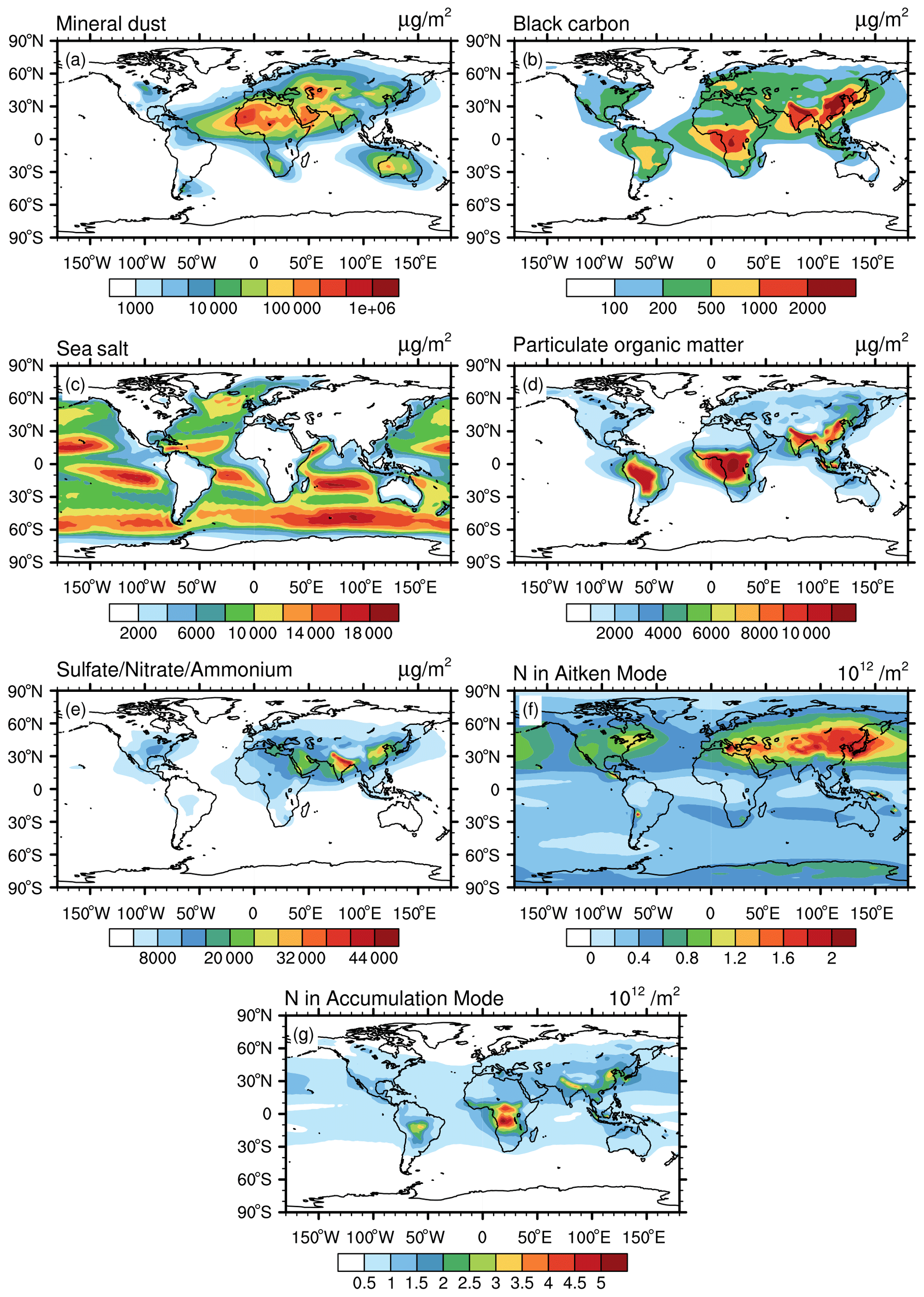
Figure 1 Simulated climatological aerosol properties for the lower troposphere (surface to ∼700 hPa), including vertically integrated mass concentration of mineral dust (a), BC (b), sea salt (c), POM (d), and SNA (e) and the vertically integrated particle number concentration of the Aitken mode N_akn (f) and accumulation mode N_acc (g).

As explained in Sect. 2.3, K-means classifications are conducted for a range of predefined cluster numbers k. The resulting classification is coarse at low k, while increasing k leads to increased complexity. At some point, however, the added complexity of the K-means classification does not add further information and therefore a further increase of k is not useful. Hence, choosing a proper cluster number for the K-means analysis is not straightforward. Here, we use 10 clusters for the lower troposphere based on the K-means evaluation metrics (SSE and SC) and expert judgement, as described above. SSE describes the sum of squared errors from each sample to the respective cluster centre (Eq. 3) and decreases with increasing k. For the lower troposphere, SSE decreases rapidly from k=2 up to about k=7 and then more slowly for larger k (Fig. 2a). The SC is highest at k=2, decreases between k=2 and k=4, and reaches a roughly constant level at k=5–11 (Fig. 2b). High SC value indicates that the data within the cluster are similar and they are distinct from other clusters. The optimal solution is obtained by minimizing SSE and maximizing the SC. Therefore, taking a balance between small SSE and large SC, we limit the selection of k to 9 to 11. The difference between the 9-cluster and the 10-cluster classification is that one oceanic aerosol regime in the 9-cluster classification is further divided into 2 clusters in the 10-cluster classification. The 11-cluster classification includes a tiny regime that adds little information with respect to the 10-cluster one (Fig. S1 in the Supplement). We therefore choose k=10 for the aerosol classification in the lower troposphere.

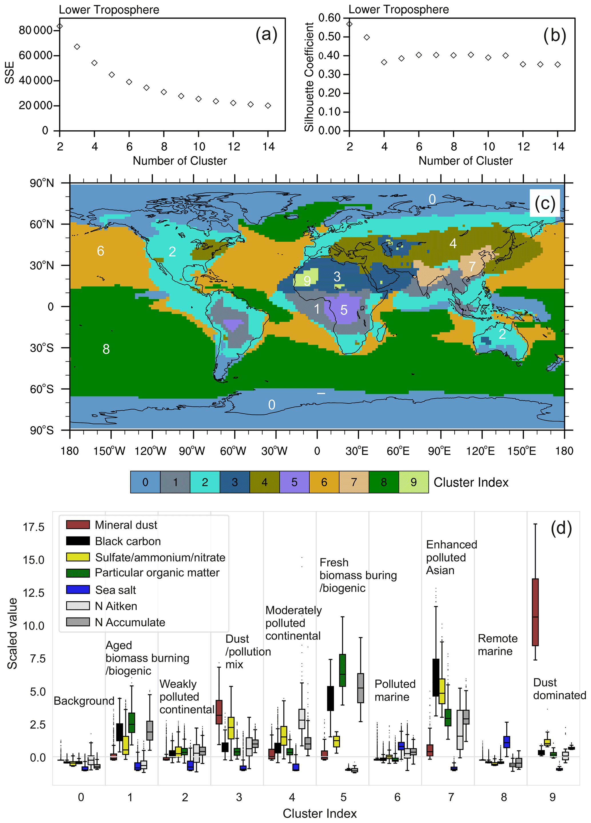
Figure 2 Lower-tropospheric clustering using K-means. The top row shows the evaluation metrics SSE (a) and SC (b) vs. a k range of 2–14. The middle row (c) highlights the spatial distribution of 10 aerosol regimes for the lower troposphere. The bottom row (d) shows the data distribution of the seven considered aerosol properties within the 10 individual aerosol regimes and cluster names assigned to each cluster based on the analysis of the aerosol data within the respective cluster. The boxplots describe the distribution of data by displaying five statistical quantities that are not outliers: the maximum value (top whisker), 75 % quantile (top of box), median (middle line in box), 25 % quantile (bottom of box), and minimum value (bottom whisker) of standardized aerosol parameters that are not outliers. The black dots are outliers, defined as the data beyond 2.67σ of a normal distribution.

The resulting 10 aerosol regimes classified by K-means for the lower troposphere are displayed in Fig. 2c. These identified major aerosol classes match well with the expected regimes in this altitude range. Polar aerosols are classified in cluster 0, while oceanic aerosols are roughly divided between Northern Hemisphere and Southern Hemisphere by clusters 6 and 8, respectively. The large forests and savannas of Africa and South America are covered by cluster 5 and cluster 1, including major biogenic and fire aerosol sources (e.g. Dentener et al., 2006). Clusters 9 and 3 cover the main desert regions over the Sahara and the Arabian Peninsula. Cluster 9 marks the strong dust emission spots, while cluster 3 represents a kind of “background desert”, which shows slight influences from aerosol transported from surrounding areas. The regions characterized by strong anthropogenic pollution (South Asia and East Asia) are assigned to cluster 7, while regions with moderate and low pollution are covered by cluster 4 and cluster 2, respectively, with the latter often extending to oceanic regions possibly affected by long-range transport of anthropogenic pollution from the continents.

The characterization of the aerosol regimes in the lower troposphere obtained with the K-means method can be further explored and interpreted using the boxplot in Fig. 2d. The figure shows the distribution of samples collected within each regime and several statistical metrics, including maximum, 75 % quantile, median, 25 % quantile, and minimum of the standardized aerosol parameters that are not outliers. We recall the use of multi-annual mean sample values and the consideration of column-integrated values in the lower-tropospheric column. The dots are outliers that can be ignored for statistical discussion. They are defined by ±1.5 times the interquartile range of the data, which corresponds to data beyond 2.67σ of a normal distribution. Note that values on the y axis are the standardized values (calculated with Eq. 5) but not the absolute value as shown in Fig. 1, in order to do a proper classification with K-means and to compare species with different units and scales. All aerosol properties within cluster 0 (polar regions) show lower values than in the other clusters, meaning that this can be considered aerosol background, as also denoted in Fig. 2d. Low values are also found in clusters 6 and 8, with the exception of sea salt, which has enhanced values. We therefore mark these two clusters as oceanic aerosol. Clusters 6 and 8 are very similar, which explains why they are merged into one cluster if a 9-cluster (instead of 10-cluster) classification is used. The difference between them is the slightly higher values of aerosol properties other than sea salt concentrations within cluster 6, which points to a more polluted marine regime than in cluster 8, which represents remote oceanic regions. Clusters 1 and 5 cover the major forests and savannas in Africa and South America and downwind areas and are characterized by enhanced POM, BC, and N_acc, which are all typical indicators of strong biomass burning and biogenic activity. The difference between the two clusters is that the enhancement of these quantities is more pronounced in cluster 5 compared to cluster 1. This difference suggests that fresh biomass burning and biogenic aerosol characterize cluster 5, while more aged particles are found in cluster 1 as a result of long-range transport and the subsequent dispersion of the affected air masses in combination with particle wet and dry deposition. Cluster 9 and cluster 3 both show enhanced mineral dust values, which agrees with their locations in large deserts or in close proximity to desert regions. Cluster 9 shows much larger mineral dust values and much lower values for the other aerosol properties (in particular SNA and N_akn) than cluster 3. This suggests that cluster 9 covers the regions of localized strong dust emissions, while cluster 3 includes dust-dominated air masses that are mixed with pollution from other regions. The dominance of BC and SNA in cluster 7 matches well with the large pollution characterizing the South Asia and East Asia regions covered by this cluster. Cluster 7 also shows enhanced POM and number concentrations in both Aitken and accumulation modes. We therefore name it the enhanced polluted Asian cluster. Clusters 2 and 4 cover large parts of the Eurasian and American continental regions. Cluster 4 is more polluted than cluster 2, but both are relatively clean compared to other continental clusters nearby (e.g. the strongly polluted Asian regions). We refer to these clusters as moderately polluted continental and weakly polluted continental, respectively. Another important aspect worth noting is that continental aerosol clusters frequently propagate into oceanic regions, showing that this method is also able to capture the long-range transport of pollutants from the emission regions to the relatively clean marine environment. For example, clusters 1, 2, and 3 also cover parts of the central Atlantic Ocean, cluster 2 also appears over the Pacific Ocean near the west coast of the American continent, and cluster 4 extends over the north-western Pacific.

3.2 Middle-tropospheric clusters

The clustering analysis for the middle-tropospheric layer uses global aerosol data from about 700 to 300 hPa. As depicted in Fig. 3, this altitude range shows lower values for the column mass and number concentrations (Fig. 1). For example, the column mass of middle-troposphere mineral dust (Fig. 3a) ranges from 2×10³ to 3.4×10⁴ µg m⁻² in areas with prominent dust impact, compared to a range of 100 to 1×10⁶ µg m⁻² in the lower troposphere (Fig. 1a). This is caused by the decrease of air density during upward transport, by the dilution of the dust load due to mixing with dust-free air masses, and by possible sinks due to wet deposition. A similar reduction is also evident in the other aerosol properties. The spatial distribution patterns, however, remain the same between the middle troposphere and the lower troposphere. However, the overall patterns, in many cases, show a larger spatial extension that is caused by long-range transport and dispersion of the respective air masses.

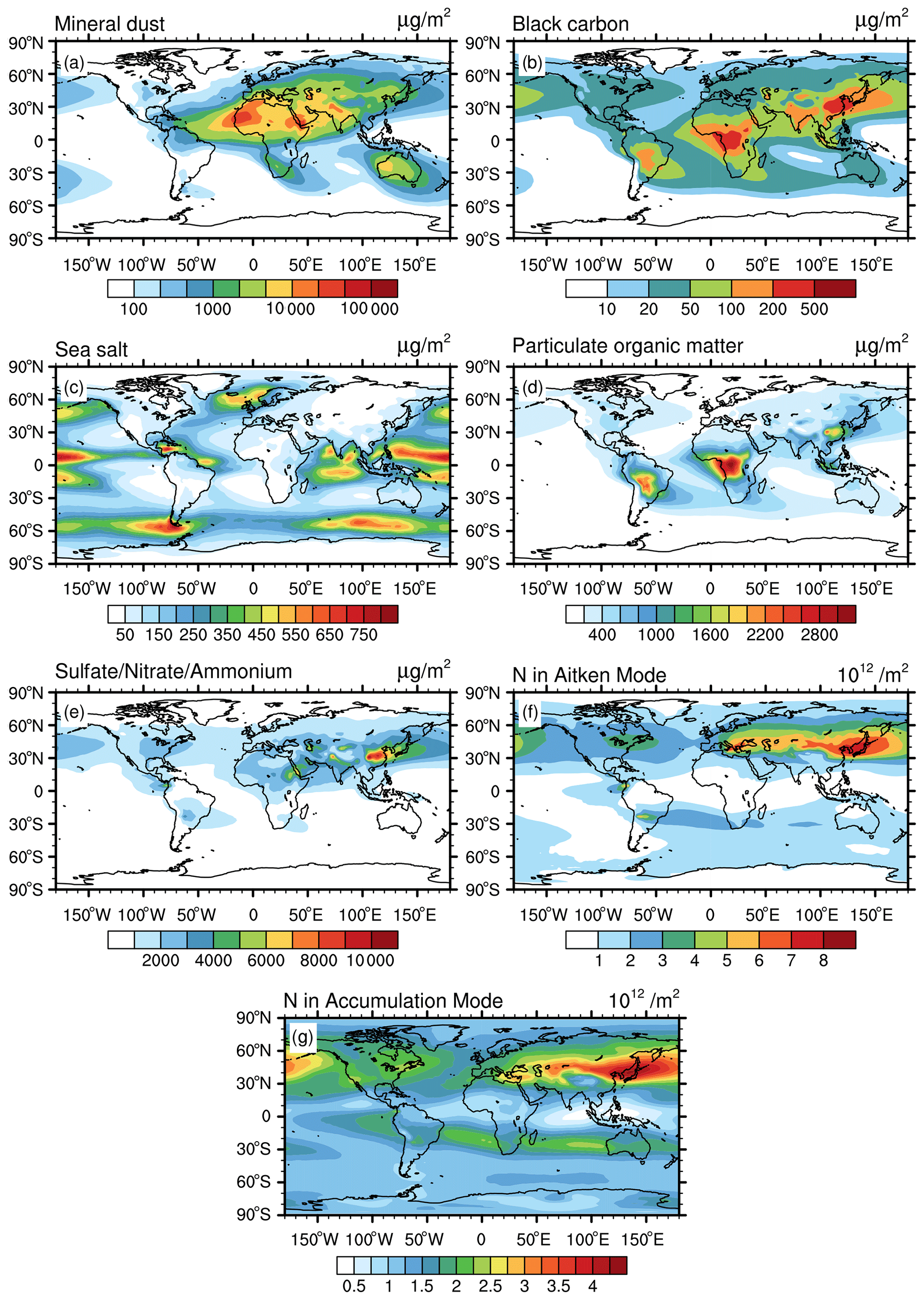
Figure 3 The same as Fig. 1 but for the middle troposphere (from ∼700 to ∼300 hPa).

Due to this dispersion, a less complex clustering is required than in the lower troposphere. In general, we can expect k to decrease with increasing altitude due to the more uniform spatial aerosol distributions in the upper-atmospheric layers. For the middle troposphere, we evaluated K-means classifications with k=2 to k=8 using the same metrics as applied above (Fig. 4a and b). As for the lower-tropospheric case, SSE decreases with increasing k but more slowly for k≥6. The SC decreases to a minimum for k=4 and increases again to a stable level between k=6 and k=8. The distribution of the major aerosol regimes becomes very robust at k=6, while only minor regimes that do not show prominent features are introduced at higher values. We therefore choose a six-cluster classification for the middle troposphere (see also Fig. S2 in the Supplement).

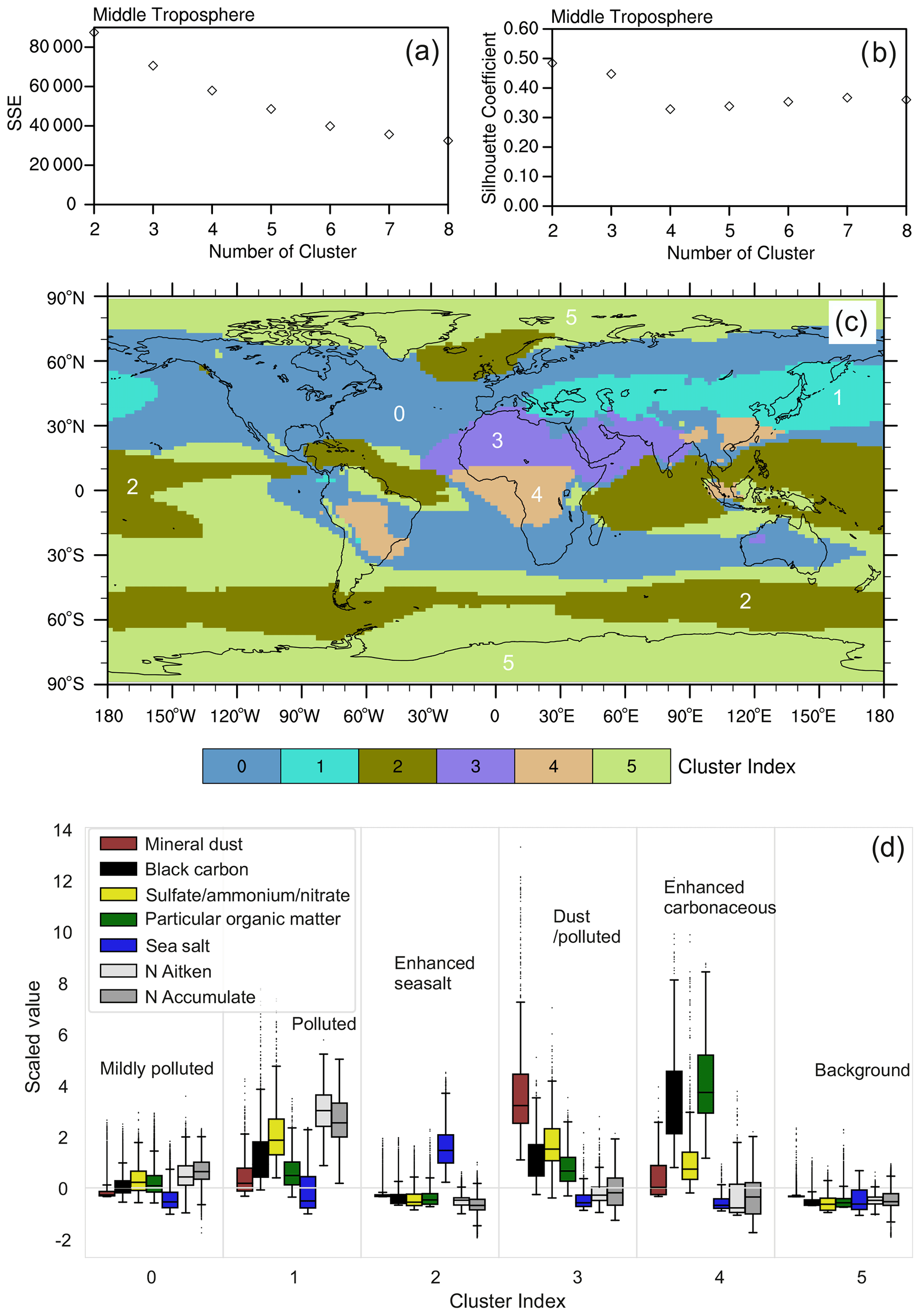
Figure 4 The same as Fig. 2 but for the middle troposphere (from ∼700 to ∼300 hPa).

In the middle troposphere, the aerosol regimes are more zonally uniform than lower down, but the lower troposphere still has a very strong influence on the pattern (Fig. 4c). The zonal uniformity particularly occurs in the case of clusters 0, 2, and 5 and appears to be related to the increasing prevalence of zonal wind patterns in the middle troposphere. Clusters 1, 3, and 4, on the other hand, show a stronger influence of the distribution of the emission sources and the transport patterns of the lower troposphere. The statistical analysis of the aerosol properties within each cluster allows the broad classification of clusters 2 and 5 as middle-tropospheric background clusters and clusters 1, 3, and 4 as middle-tropospheric polluted clusters (Fig. 4d). The lowest values of all aerosol properties are found in cluster 5, which can be classified as middle-tropospheric background (relatively clean) and covers large fractions of the Southern Hemispheric oceans and the polar regions. Cluster 2 is characterized by enhanced sea salt values, while the values of other aerosol species remain low, as in cluster 5. Hence, the cluster includes background air enriched with sea salt due to enhanced wind-driven emissions. Cluster 2 mainly covers the intertropical convergence zone (between 20^∘ S and 20^∘ N) with its strong updraughts and the Southern Hemispheric storm track area around 60^∘ S, which is also an uplift region between the mid-latitude cell and the polar cell of the main atmospheric circulation pattern. Due to the strong upward transport in these regions, sea salt is lifted from the sea surface to the middle troposphere. Cluster 0 is mainly located in the Northern Hemisphere and above the continents: it is characterized by mildly enhanced BC, SNA, POM, N_akn, and N_acc. Similar enhancements of some of these aerosol properties are evident in clusters 1, 3, and 4 but with much larger values. These clusters show similar aerosol characteristics and cover similar regions to their counterparts in the lower troposphere (note, however, that the algorithm assigns different cluster index numbers for the lower- and middle-troposphere cases). These three polluted clusters nicely identify three distinct sources: cluster 1 is mostly affected by the strong emission regions in South Asia and East Asia and Southern Europe and the Mediterranean Sea, cluster 3 presents a mixture of mineral dust and other pollution sources (with an evident prominence above large deserts), and cluster 4 is an enhanced carbonaceous and biogenic cluster with significant coverage over biomass burning and biogenic sources, e.g. in South America and Africa. It also occurs over East Asia, with its high anthropogenic emissions of carbonaceous particles. Note that the scaled values in Figs. 2d and 4d should not be compared directly among the different atmospheric layers because the input data for K-means analyses are scaled individually based on the data within each layer.

3.3 Tropopause region clusters

The clustering analysis for the tropopause region considers global aerosol data from about 300 to 100 hPa. The degree of spatial dispersion again increases when compared to the lower layers. Therefore, the distributions become more homogeneous than in the middle and lower troposphere (Fig. 5). The maximum values of the five aerosol mass columns (mineral dust, BC, sea salt, POM, SNA) are lower in the tropopause region (Fig. 5) than their background value in the lower troposphere (Fig. 1). For example, the maximum mineral dust mass column in the tropopause region amounts to about 1×10³ µg m⁻², which is close to the minimum value of mineral dust in the lower troposphere. Although aerosol mass columns in the tropopause region are generally small and a high degree of dispersion is reached, the spatial patterns for mineral dust, BC, POM, and SNA are still related to those in the lower troposphere. This demonstrates that local upward transport of aerosols from the Earth's surface to the tropopause region is efficient in areas showing enhanced dust concentrations. However, this does not fully apply to sea salt, which reaches high values only in the tropics corresponding to regions of strong convection over the oceans into the tropopause region (Fig. 5c). With regard to the aerosol number columns, the effects of vertical and zonal transport appear to be more complex. While the accumulation mode particle number shows a similar behaviour to the mass loadings, the Aitken mode particle number column appears to be strongly influenced by new particle formation in the tropopause region. Hotspots of the particle number particularly occur over regions of enhanced gaseous pollution that provides aerosol precursor gases, such as SO₂, leading to aerosol nucleation and growth favoured by the clean environment of the tropopause region.

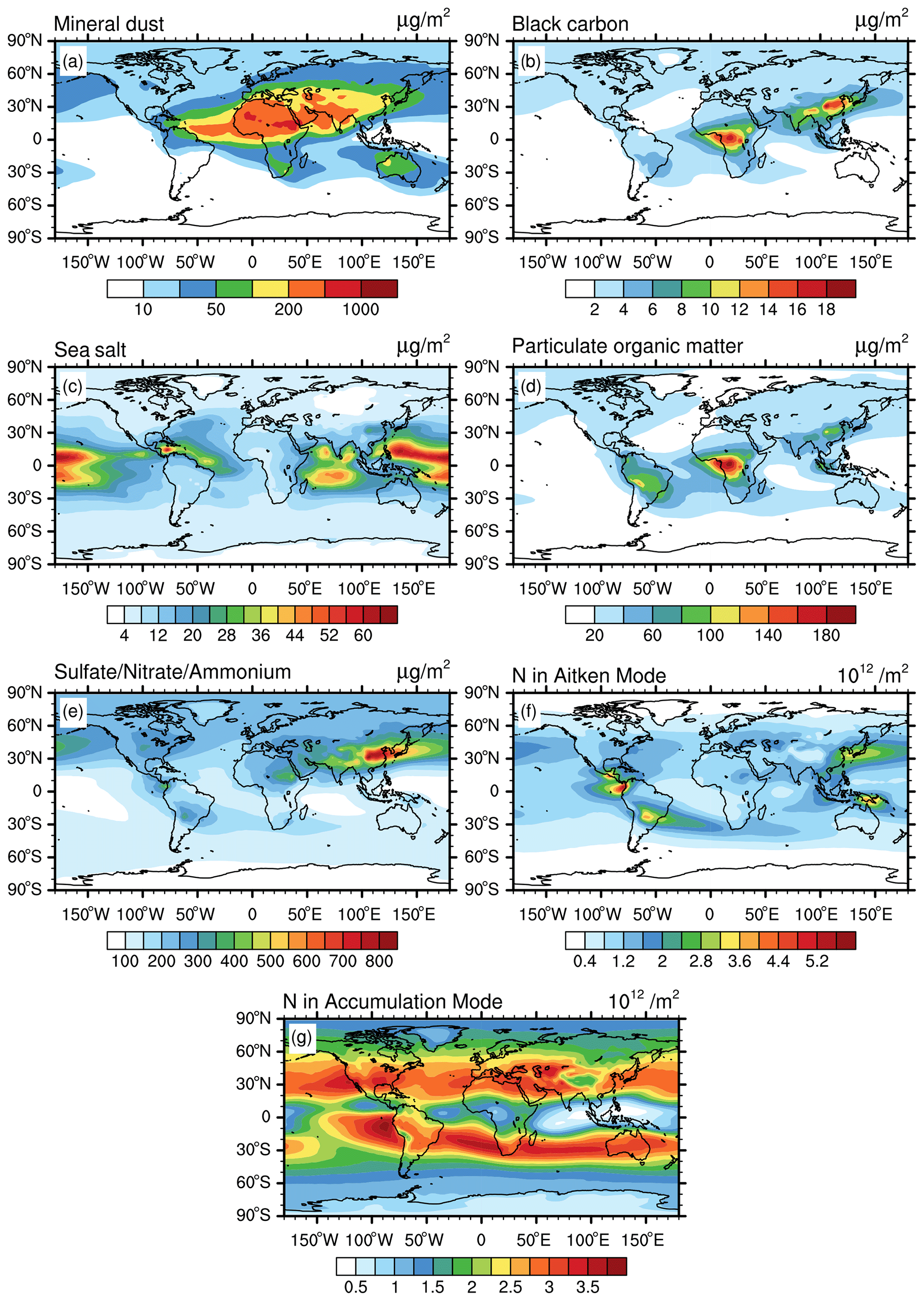
Figure 5 The same as Fig. 1 but for the tropopause region (from ∼300 to ∼100 hPa).

As mentioned above and favoured by the homogeneous characteristics of aerosol in the tropopause region shown in Fig. 5, a more simplified clustering can be applied in this layer, reducing k to less than 6. Aerosol cluster distributions for a range of different k are shown in Fig. S3 in the Supplement. The SSE of K-means clustering for the tropopause region (Fig. 6a) shows a similar structure to that in the middle troposphere (Fig. 4a), with noticeable convergence from about k=6. The SC reaches a maximum for k=4 and k=5 (Fig. 6b). The combination of these two metrics suggests k=5 is the proper choice for the K-means classification for the tropopause region. The resulting five clusters are shown in Fig. 6c. Large parts of the tropopause region belong to cluster 1, which covers both polar regions and most of the southern extra-tropics. The second largest cluster is cluster 2, which covers a large part of the northern extra-tropics and about half of the tropical ocean regions, with the other half mostly covered by cluster 3. Clusters 0 and 4 cover a small portion of the continents, including central Africa, the Saharan region, and tropical and subtropical Asia. Figure 6d highlights the aerosol characteristics for each cluster of the tropopause region. Cluster 1 shows the lowest values for all aerosol properties which suggests that it should be characterized as tropopause region background. Note that in the polar regions the pressure levels considered here are mostly located in the stratosphere and therefore contain comparably clean air. Cluster 3 shows similarly low values for all species except for sea salt, which is significantly enhanced due to upward transport in the intertropical convergence zone. Hence, we denote it as the tropopause region enhanced sea salt cluster. The slightly enhanced N_acc in cluster 3 relative to cluster 1 is probably caused by new particle formation. Cluster 2 shows slight increases for all aerosol properties relative to cluster 1 but is still lower than in the other clusters. We therefore define cluster 2 as the tropopause region mildly polluted cluster. Cluster 0 features strongly increased mineral dust accompanied by slight increases in BC and SNA. Therefore, it can be termed tropopause region dust/polluted cluster. This is also supported by its geographical location over the Sahara and the Middle East, where mixtures of desert dust with anthropogenic pollution could be expected. Cluster 4 shows strongly enhanced BC, SNA, and POM and mildly enhanced mineral dust, which suggests that this regime should be termed the tropopause region polluted/mixed cluster. On the one hand, it is strongly influenced by the biomass burning and biogenic aerosol sources over central Africa and South America. On the other hand, it also shows relevant coverage over East Asia resulting from the strong pollution sources in these regions. Note that there are many similarities between the aerosol regimes of the tropopause region and the middle troposphere (Fig. 4), especially for clusters 3 and 4, which are largely controlled by efficient updraughts. Hence, these clusters also correspond well to lower-tropospheric aerosol regimes with similar characteristics occurring in the same regions (Fig. 2).

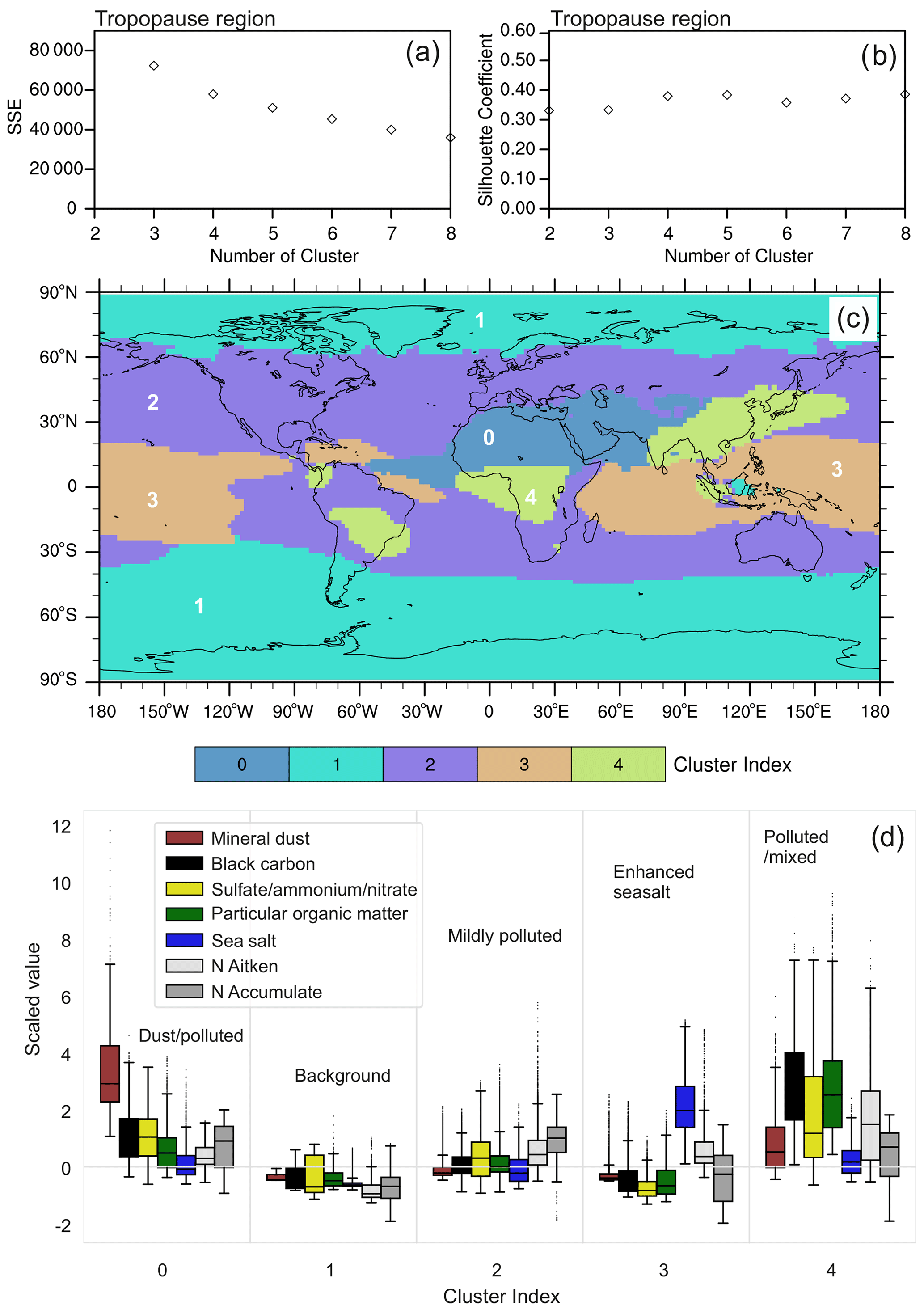
Figure 6 The same as Fig. 2 but for the tropopause region (from ∼300 to ∼100 hPa).

4 Discussion

4.1 Effects of scaling methods on K-means clustering

Since the choice of the variance applied for data scaling could potentially have an effect on the clustering, we investigate the influences of different scaling methods on our results in this section. Table 1 summarizes the five tested scaling methods: S1 is the reference standardization method chosen in this study. It is based on Eq. (6). S2 is similar to S1 but applied to the base-10 logarithm of the input data. S3–S5 are alternative methods based on different statistical metrics for standardizing the data. The sensitivity test is applied to the data from the lower troposphere, as this domain is characterized by a larger spatial variability than the middle- and upper-atmospheric layers, hence more pronounced clustering features can be expected. As an example, we use the 10-cluster distribution. The optimal selection of k could vary among the different standardization approaches, but we choose a fixed value of k to analyse the impact on the results solely due to the standardization method. The selection of an optimal value for k will be addressed again using a different approach in the next section.

Table 1 Summary of the different scaling methods applied in this work.

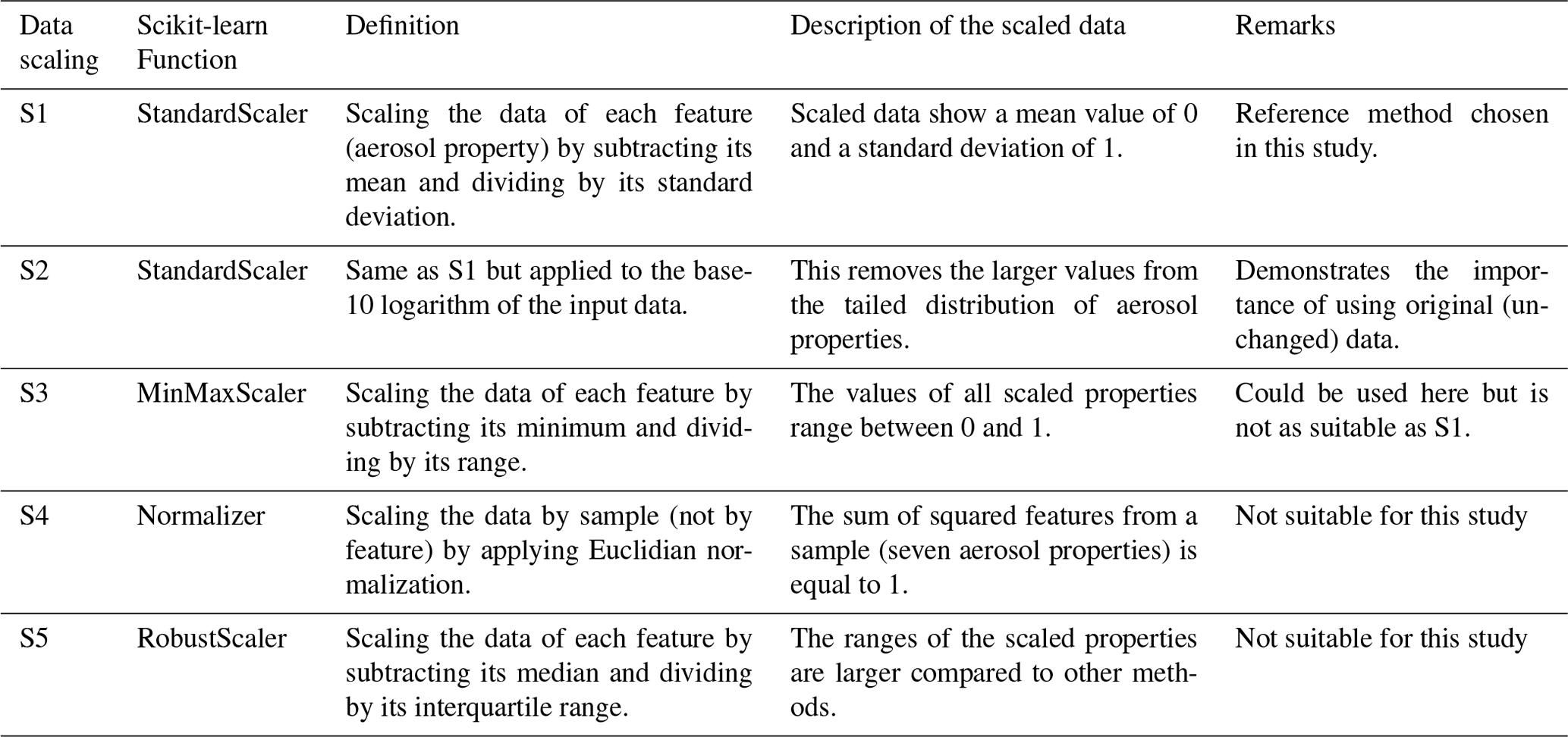
Figure 7 compares the probability density functions (PDFs) of the raw input data and the scaled data using the different standardization methods summarized in Table 1. Figure 8a–e show the distribution of clusters resulting from the differently scaled data and demonstrates how data scaling changes the results of K-means clustering. Based on these results, we can draw the following four conclusions. (1) The standardization that we use for this study (S1) simply scales the values of aerosol properties, but it does not change the underling distribution of the raw data (see the first and second column in Fig. 7). (2) The most important criterion for K-means data preprocessing is that the data of different properties should be scaled to a comparable range so that they are more or less equally weighted. This is clearly not achieved when using the standardization methods S4 and S5, leading to a large spread in the ranges of scaled data for different aerosol properties (last two columns in Fig. 7). For example, using the S4 method, the maximum scaled value of N_akn and N_acc is 1.0, while for the other five aerosol properties the maximum values are smaller than $\mathrm{6.0}\times {\mathrm{10}}^{-\mathrm{13}}$ (Fig. 7, fifth column). Similarly, using the S5 method results in much larger values for mineral dust compared to the other aerosol properties (Fig. 7, sixth column). As a consequence, the properties with larger values are weighted more strongly in the K-means clustering, leading to a classification largely dominated by these properties (compare Figs. 1a and 8e). (3) Both the S1 and the S3 methods scale the data to comparable ranges and retain the underlying distribution of the input data, but S1 is more appropriate for this study. For example, sea salt is a natural marine aerosol and its global range of concentration values is relatively narrow in comparison to the global ranges of other types of aerosols that have both anthropogenic and natural sources or pure natural sources but with locally strong emissions as mineral dust. The maximum values of global sea salt correspond to about 3 standard deviations, while the maximum values of other aerosol properties correspond to about 10–18 standard deviations (Fig. 7, second column). This difference is a true feature of the data. Therefore, scaling sea salt and other aerosol properties to the same range of values between zero and one using the S3 method is not suitable for the purpose of this study since it leads to comparably large weighting of sea salt. The difference in the resulting clusters using the S1 and S3 methods are depicted in Fig. 8: the S3 method (Fig. 8c) results in finer defined clusters over the Southern Hemispheric ocean regions compared with S1 (Fig. 8a), but this is at the expense of a less detailed clustering over the continental regions. For the purpose of this study, however, these fine-resolved oceanic clusters are less relevant than a better-defined continental clustering. Furthermore, sharply defined Southern Hemisphere clusters could also be achieved by increasing k using S1 data (Fig. S1). (4) The “outliers” in the data distribution are important for aerosol clustering. We tested this by applying the base-10 logarithm to the original (skewed) distribution, resulting in a more Gaussian-like distribution (Fig. 7, third column) and thus removing the outliers. When applying the K-means algorithm with this method, several polluted clusters vanish (compare Fig. 8a and b). Although the basic structure of clusters is still visible, some important information is not captured with the S2 method. For the purpose of the present work, these high values in the data distribution should not be interpreted as outliers in the general sense, i.e. indicating noise and incorrect information that could hinder K-means clustering, but instead as features resulting from the intrinsically large spatial differences of aerosol properties across the globe, which provides useful information about the data set. It is also important to recall that we consider climatological data averaged over a long-term period (14 years), which already excludes unrepresentative high values in the aerosol distribution.

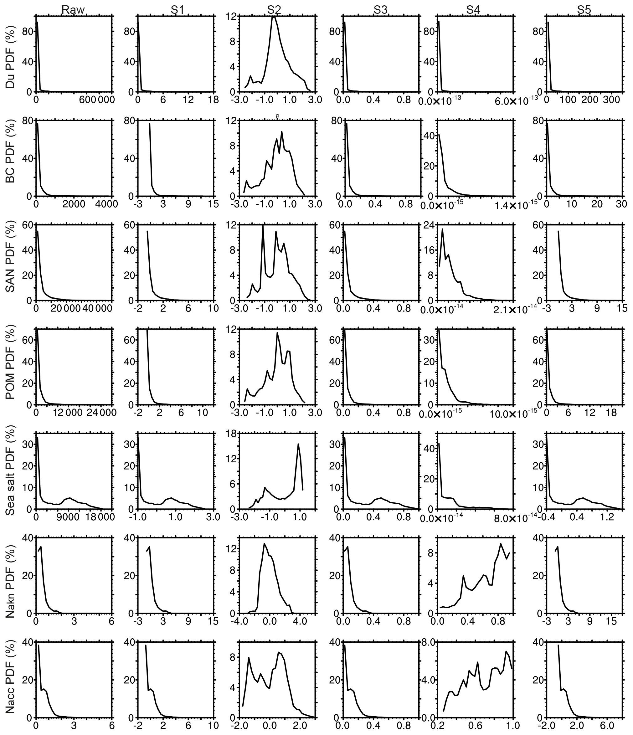
Figure 7 Probability density functions (PDFs) of the seven aerosol properties (rows) derived from their global lower-tropospheric distributions in the raw (unscaled) data (first column) and after applying the S1–S5 scaling methods (second to sixth column). The units of the raw (unscaled) values are the same as in Fig. 1.

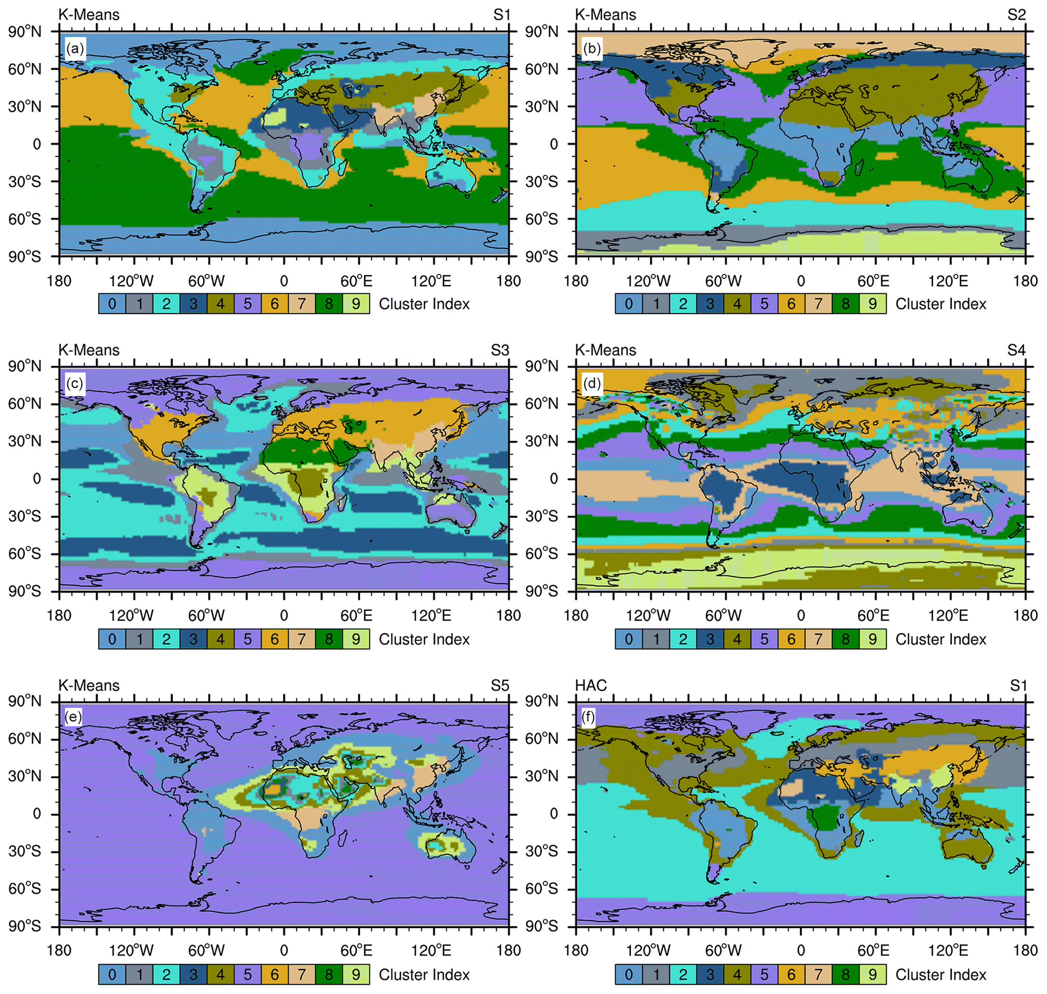
Figure 8 Comparison of K-means 10-cluster distributions based on data scaled with methods S1–S5 (a–e, respectively). Panel (f) shows the HAC clustering method combined with the S1 method.

Based on this sensitivity analysis, we conclude that the StandardScaler (S1) standardization method is the most appropriate one for the scope of this study. Although we focus in this section on the lower troposphere, this conclusion holds for the middle troposphere and tropopause region as well (see Figs. S4–S7 in the Supplement).

4.2 Comparison of K-means and HAC clustering

As with K-means, HAC clustering belongs to the family of unsupervised clustering algorithms. It works with techniques based on hierarchical clustering schemes (e.g. Müllner, 2013). More specifically, HAC treats all samples as individual clusters in the first step, and then it successively merges the pair of clusters which are closest to each other in Euclidean distance until all samples are grouped into a single cluster. In contrast to K-means, which requires a prescribed number of clusters k and separate metrics to evaluate a selection of optimal k, HAC shows the hierarchy of clustering along a workflow (the so-called dendrogram), which allows a selection of reasonable cluster numbers based on this hierarchical structure.

In this section, we compare results of aerosol clustering with HAC and K-means, using the StandardScaler (S1) standardization method and focus on the lower troposphere as an example (additional results for the middle troposphere and tropopause region are provided in the Supplement). The way HAC clustering handles the data points is called linkage. There are different linkage methods, such as “Ward”, “Single”, and “Maximum”. Here we apply the Ward linkage method for HAC clustering since it minimizes the sum of squared differences within all clusters and is therefore similar to the K-means approach. The truncated dendrogram of HAC clustering for the lower-tropospheric aerosol is shown in Fig. 9. It demonstrates the path from grouping all samples as individual clusters to one single cluster, and provides insights into the similarities and differences between individual data points or clusters. The distance between two clusters (vertical axis) on the bottom of the hierarchy structure is small but increases as the number of clusters decrease. At a certain level, the dendrogram can be cut in correspondence with the chosen number of clusters. This choice, however, is also subjective and lies in the hand of the investigator. Our selection of 10 clusters is supported by the dendrogram plot, which shows a distinct distance between clusters at this level and is also consistent with the selection of 10 clusters for K-means clustering.

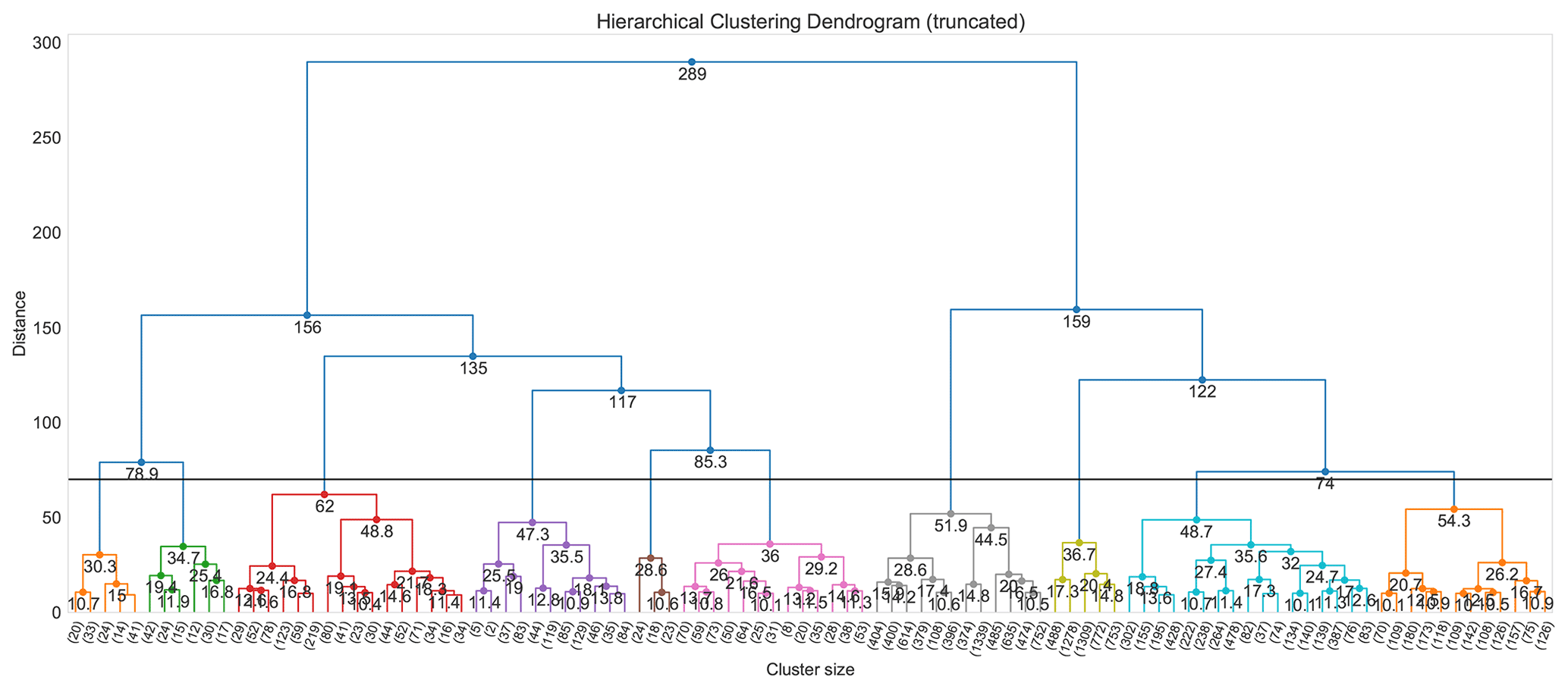
Figure 9 Dendrogram plot of HAC clustering for lower-tropospheric aerosols. Since the number of samples (96 latitude × 192 longitude points, resulting in 18 432 samples) is too large to be shown on a single plot, the dendrogram is truncated to display only the path of grouping starting from 100 clusters. The values on the horizontal axis represent the number of samples for each branch of these 100 clusters. The horizontal line marks our selection of the cluster number (i.e. k=10). The distance (y axis) measures the Euclidean distance between different clusters. The average distance of the merged clusters is highlighted below the clusters.

The cluster distribution of K-means and HAC shows a good overall agreement but also small differences (Fig. 8a and f). We see similarities in the background clusters at the polar regions, the mildly polluted oceanic cluster at northern latitudes, the clean oceanic cluster at southern latitudes, and the continental polluted clusters (dust cluster, biogenic cluster, Indian cluster, and southeastern China cluster). Differences are visible, e.g. in the size of the biogenic cluster over South America and the size of the mildly polluted continental cluster over the eastern USA. Interestingly, the extent of biogenic clusters over Africa and other continental clusters over Europe and Asia seems to be identical in the two cases. These fine differences in cluster size could be a result of K-means clustering the data by trying to separate samples in groups of equal variances, which HAC does not.

Another aspect to be considered when comparing these two clustering algorithms is the computational expenses. K-means is a fast algorithm. Its computing cost does not scale considerably with sample size or dimensions. HAC has a higher demand on computing time than K-means, especially when the sample size is large. For a sample of size n, the computing cost of HAC scales approximately as n² (Dasgupta, 2016; Roy and Chakrabarti, 2017). This is because the hierarchical clustering considers all possible merges at each step, resulting in a rapidly increasing computing time for larger samples. However, HAC features a hierarchy structure (dendrogram), which is more informative and straightforward for deciding on the number of clusters to be used. For this study, both methods provide similar results. Considering further applications of clustering in more complex situations, we chose K-means primarily due to its computational performance.

4.3 Strength and limitation of global aerosol simulation

The major goal of this study is the development of a clustering method to complement classical approaches for analysing and interpreting global aerosols model output. In order to put the demonstration results of the method presented in Sect. 3 in the right context, strengths and limitations of global aerosol simulations are discussed in the following.

Extensive evaluations have been conducted in previous studies to investigate the potential of global aerosol simulations and their limitations (e.g. Textor et al., 2006; Lauer et al., 2007; Bauer et al., 2008; Koch et al., 2009; Mann et al., 2010, 2014; Pringle et al., 2010; Aquila et al., 2011; Huneeus et al., 2011; Kirkewåg et al., 2013, 2018; He and Zhang, 2014; Koffi et al., 2015; Lee et al., 2015; Michou et al., 2015; Kaiser et al., 2019). A major deficiency of global aerosol simulations is their inability to resolve small-scale and localized processes, largely as a result of the computational challenges and the chemical complexity allowing for only coarse grid resolution in global models. Our clustering analysis is based on data from a global model simulation performed with EMAC-MADE3. The data used have a spatial resolution of about $\mathrm{1.9}{}^{\circ }\times \mathrm{1.9}{}^{\circ }$ in latitude and longitude and can therefore not reproduce smaller-scale features, such as aerosol pollution on the scale of specific cities. However, the focus of the present study is the analysis of large-scale global climatological aspects with high relevance for simulating aerosol climate effects. Investigating localized aerosol phenomena and their temporal evolution, which would be of particular relevance for air pollution aspects, is not the intention.

Global aerosol simulations mostly capture the major large-scale spatial patterns of aerosol properties well. For the EMAC-MADE3 model applied here, this was demonstrated by Kaiser et al. (2019) and Beer et al. (2020). Hence, the clustering results can also be expected to show the major large-scale features of the global aerosol distribution. One should keep in mind that for K-means clustering the distribution of data is more important than their actual value. Despite the detailed evaluation and improvement of EMAC-MADE3, some model biases and deficiencies remain and could affect the outcome of the clustering algorithm (Kaiser et al., 2014, 2019; Beer et al., 2020). However, model systematic biases are not necessarily related to incorrect data distribution. The model mostly captures the spatial patterns of the aerosol properties, and thus their actual values can be biased. Systematic biases in model parameterizations and also probably boundary conditions such as the considered emission rates (e.g. overestimation or underestimation) cause errors in the absolute values of simulation variables, but these errors mostly cancelled out when the data are standardized for the K-means analysis. However, simulation biases in the spatial patterns would change the identified regimes. The extent of such effects needs to be further investigated in future studies.

The key advantages of global aerosol simulations are the self-consistent representation of a large number of various aerosol species and properties, the possibility of generating long-term climatological information and future projections, and the global three-dimensional spatial coverage from the surface to the upper atmosphere. This provides a well-suited database for clustering algorithms. Due to model deficiencies, the clusters derived from the model output could deviate from their appearance in the real atmosphere. However, applying the same algorithm to observational data is not feasible, since no data set including all relevant chemical and microphysical aerosol properties with global coverage and vertical resolution exists. Vertically resolved data are available from in situ aircraft-based measurements, but their geographical coverage is limited, and they are often not representative for the climatological scale. Satellite data could in principle provide global coverage, but they usually comprise optical aerosol properties, such as aerosol optical depth or aerosol extinction (e.g. Popp et al., 2016). Optical aerosol quantities could be used for classification (e.g. Groß et al., 2015), but the resulting classes do not necessarily reflect the details of aerosol composition and size. In this context, using global model simulation data for classifying global aerosol regimes is an appropriate strategy.

The extensive evaluation performed in the existing global aerosol model studies, considering very large numbers of aerosol-related quantities represented in the simulations, is often difficult to interpret. This in turn suggests that new analysis methods (e.g. treating aerosols as groups, as presented in this study) are in demand. Although aerosol classification is developed in this study primarily for evaluation purposes, the results of aerosol classification from the global model output potentially provides valuable insights for aerosol research, taking the advantages and limitations of global aerosol simulation into consideration.

4.4 Limitations and potential application of K-means clustering

This study demonstrates the successful application of the K-means algorithm for the classification of global aerosol climatological regimes in model simulation output. It provides quantitative information about the aerosol regimes across the globe and at three altitude ranges from the surface to the tropopause region. The clustering analysis performed by the algorithm allows for the systematic characterization of many aerosol properties in a single index, facilitating the analysis of the output of global model simulations. This study represents a first attempt to apply the clustering method to global aerosol modelling. However, it of course has limitations and potential for improvement. These are discussed below, together with suggestions for possible applications of the presented method.

The K-means method has advantages and disadvantages in performing classification tasks. The advantage is that it does not require prior classification knowledge or training data (Hastie et al., 2009). In cases where no detailed concepts for a pre-definition of aerosol classes based on primary aerosol model parameters can be provided, using K-means is a proper approach. The disadvantage is that the K-means method is sensitive to data variability. Our calculations demonstrated, for instance, that a too high variability resulting from the consideration of temporal variation complicates the K-means clustering. Beyond the analysis of multi-annual means, we attempted to classify global climatological seasonal data that include the variability in the time dimension concerning the four seasons. This attempt resulted in complications in the classification across the four seasons, since in many cases the seasonal variations are larger than the differences between the specific clusters, which leads to large changes in the characteristics of the clusters and their spatial extent from season to season. This shows that the K-means method discussed here does not work well for analysing the data variability across time and space simultaneously, as the interpretation of the resulting classification would be challenging. To overcome this limitation, we removed the variability in the time dimension in this study by considering multi-year averages of the model output, thereby setting a focus on classifying the spatial distribution of long-term climatological aerosol regimes. Possible inter-annual and seasonal variability of aerosol properties could alternatively be discussed on the basis of the climatological regimes analysing the internal temporal changes of aerosol properties within the climatological clusters obtained by K-means.

Despite its limitations, the K-means method presented in this study could be a very helpful tool to analyse and interpret the huge amount of aerosol data generated by global simulations, including detailed descriptions of the size-resolved aerosol composition. The method has a wide application potential. Since the algorithm identifies aerosol regimes by minimizing the variance within each cluster, the aerosol properties at different locations within a cluster are similar. This implies that aerosols can be treated cluster-wise instead of grid-point-wise, thus reducing the amount of data required to describe the global aerosol population. Possible applications of this method include (but are not limited to) the following.

1. Investigating and correcting model systematic biases using observational data is an important aspect in aerosol model development. However, it is often challenging due to the limited temporal and spatial coverage of observational data. Using the K-means algorithm to identify major aerosol regimes allows for the simplification of bias-adjustment approaches, since even spatially limited observations within a given cluster can be used to adjust the biases in other regions of that regime. In this context, only systematic model biases that occur nearly homogenously throughout the whole cluster (and not purely local model discrepancies) should be addressed. The bias adjustment for global aerosols nevertheless remains difficult since it requires a systematic compilation and homogenization of observational aerosol data from different sources, instruments, and regions and requires the consideration of various observational uncertainties. This is planned for a follow-up study.

2. The identified aerosol clusters can be used as first-order criteria for satellite retrievals. Some satellite retrieval algorithms (Holzer-Popp et al., 2008; Kahn and Gaitley, 2015) first calculate aerosol optical depth for several pre-defined aerosol types and compositions with top-of-atmosphere reflectance look-up tables and then select the best spectral or multi-angular fit between calculated and observed microphysical and optical top-of-atmosphere reflectance from the different aerosol types in the atmosphere. This is a time-consuming process since a large number of different aerosol types and compositions need to be tested (e.g. 36 or 74 mixtures) without any a priori pre-selection. By applying the results of the clustering method presented here the characteristics of each aerosol regime could be used to dismiss unrealistic guesses before applying the retrieval algorithm, thus reducing the computing time.

3. Our results could provide data for training other supervised machine learning algorithms. K-means is chosen in this study because a priori definition of aerosol classes is not straightforward since it would require a thorough analysis of the prevailing aerosol regimes in the model output. This is, however, intended to be achieved with K-means. But if the prevailing aerosol regimes are known from the K-means results, it is possible to prepare training data sets for other supervised machine learning algorithms for further, more detailed classifications, e.g. using random forest or neural network approaches.

4. The planning of future observational campaigns could benefit from model-based cluster analyses, as they provide useful information about aerosol characteristics in different regimes. Based on this information, campaign planners could easily identify regions of interest regarding specific aerosol properties or types, for example focusing on aerosol from specific sources (e.g. mineral dust from deserts or particles from biomass burning regions).

5. Possible long-term aerosol trends could be analysed by comparing the distribution of clusters calculated for different periods (e.g. pre-industrial conditions, present-day conditions, and future scenarios), which would also provide insights for the validation of climate and air quality measures.

5 Summary and outlook

In this study, we apply the K-means algorithm to classify climatological aerosol regimes across the atmosphere, primarily for evaluation purposes, based on seven primary aerosol properties simulated with the EMAC-MADE3 global aerosol model. These properties include mass concentrations of black carbon, mineral dust, sea salt, particulate organic matter, and the sulfate–nitrate–ammonium system and the aerosol number concentrations of the Aitken and accumulation modes. K-means classifies the model data by means of a cluster analysis based on a minimization of the variances, and thus data within a respective cluster are similar to each other but different to those in other clusters. K-means is especially useful when prior classification knowledge is not available. We apply K-means to quantitatively identify global aerosol regimes and explain the characteristics of the classified regimes regarding their location, extent, and specific aerosol properties. This study represents the first application of this algorithm for aerosol classification in global model output. The results show that the lower-tropospheric aerosol regimes are largely controlled by emissions. Different aerosol clusters are identified and are characterized by biomass burning or biogenic activity, mineral dust, anthropogenic pollution, background conditions, and a mixture of these different types. Several continental clusters propagate over the oceans due to long-range transport of the affected air masses. The algorithm classifies the oceanic regions into two major clusters: a moderately polluted Northern Hemisphere and a cleaner Southern Hemisphere. In the middle troposphere and the tropopause region the aerosol regimes are more zonally uniform than near the surface, but the lower troposphere has still a very strong influence on the pattern, especially in the case of the three polluted clusters occurring over Africa, South Asia, and East Asia. Due to efficient vertical dispersion, these clusters are present at all altitude levels and show similar characteristics from the surface to the tropopause region.

The above results need to be interpreted keeping the limitation and strength of global aerosol models in mind. Due to the complexity of the processes they simulate in combination with the global, long-term coverage, these models are operable only with a relatively coarse grid resolution (on the order of 100 km). Hence, they cannot explicitly represent smaller-scale processes but need to rely on parameterized representations instead. They are, however, a valuable tool to capture the large-scale spatial pattern of aerosol properties, which supports the idea that our results could provide useful insights for aerosol studies.

Two sensitivity tests have been conducted in this study to investigate the robustness of the presented method. Firstly, we investigate how data scaling influences the K-means classification. By comparing five different data-scaling approaches, StandardScaler (S1) standardization proved to be an appropriate data pre-processing method for this study. Secondly, we explored the differences in classifications purely due to applying an alternative classification algorithm. To this end, the K-means results are compared to the output of another unsupervised classification algorithm (HAC). The results of the classification from both algorithms show good agreement, with only small differences in cluster sizes, but the higher computational efficiency of K-means makes it the preferred algorithm for clustering the large data samples resulting from global aerosol model output.

The classification of global aerosol has a wide spectrum of potential applications. We have suggested several possible future applications that could benefit from this classification scheme. These include identifying model biases, conducting bias adjustments, preparing training data for other supervised classification algorithms, simplifying satellite retrieval processes, and supporting campaign planning.