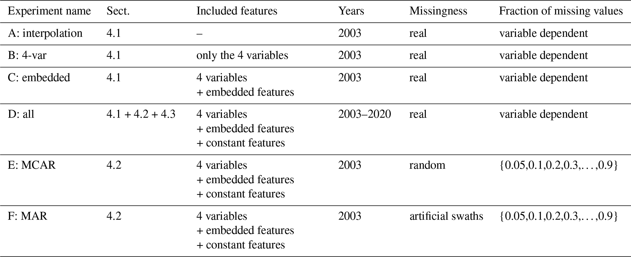
the Creative Commons Attribution 4.0 License.
the Creative Commons Attribution 4.0 License.
 | 14 Jun 2022
CLIMFILL v0.9: a framework for intelligently gap filling Earth observations
Verena Bessenbacher
Sonia Isabelle Seneviratne
Lukas Gudmundsson
Remotely sensed Earth observations have many missing values. The abundance and often complex patterns of these missing values can be a barrier for combining different observational datasets and may cause biased estimates of derived statistics. To overcome this, missing values in geoscientific data are regularly infilled with estimates through univariate gap-filling techniques such as spatial or temporal interpolation or by upscaling approaches in which complete donor variables are used to infer missing values. However, these approaches typically do not account for information that may be present in other observed variables that also have missing values. Here we propose CLIMFILL (CLIMate data gap-FILL), a multivariate gap-filling procedure that combines kriging interpolation with a statistical gap-filling method designed to account for the dependence across multiple gappy variables. In a first stage, an initial gap fill is constructed for each variable separately using state-of-the-art spatial interpolation. Subsequently, the initial gap fill for each variable is updated to recover the dependence across variables using an iterative procedure. Estimates for missing values are thus informed by knowledge of neighbouring observations, temporal processes, and dependent observations of other relevant variables. CLIMFILL is tested using gap-free ERA-5 reanalysis data of ground temperature, surface-layer soil moisture, precipitation, and terrestrial water storage to represent central interactions between soil moisture and climate. These variables were matched with corresponding remote sensing observations and masked where the observations have missing values. In this “perfect dataset approach” CLIMFILL can be evaluated against the original, usually not observed part of the data. We show that CLIMFILL successfully recovers the dependence structure among the variables across all land cover types and altitudes, thereby enabling subsequent mechanistic interpretations in the gap-filled dataset. Correlation between original ERA-5 data and gap-filled ERA-5 data is high in many regions, although it shows artefacts of the interpolation procedure in large gaps in high-latitude regions during winter. Bias and noise in gappy satellite-observable data is reduced in most regions. A case study of the European 2003 heatwave shows how CLIMFILL reduces biases in ground temperature and surface-layer soil moisture induced by the missing values. Furthermore, in idealized experiments we see the impact of fraction of missing values and the complexity of missing value patterns to the performance of CLIMFILL, showing that CLIMFILL for most variables operates at the upper limit of what is possible given the high fraction of missing values and the complexity of missingness patterns. Thus, the framework can be a tool for gap filling a large range of remote sensing observations commonly used in climate and environmental research.
- Article
(19046 KB) - Full-text XML
- BibTeX
- EndNote


1.1 Missing observations in Earth system science
Observing the Earth surface from space is an endeavour that has significantly contributed to advance our understanding of the Earth system and has played a vital role in the fields of data assimilation (Bauer et al., 2015), Earth surface modelling (Balsamo et al., 2018), global freshwater hydrology (Lettenmaier et al., 2015), global carbon cycle processes (Humphrey et al., 2018), and the study of climate extremes in the land–atmosphere system (Dorigo et al., 2017; Nicolai-Shaw et al., 2017; Teuling et al., 2010). A plethora of instruments observes variables relevant for determining the state of the Earth remotely at any given time. However, this observational record is highly fragmented: remote sensing observations have a extensive spatial coverage but differ in their spatial and temporal resolution and their frequency and temporal extent or suffer from inhomogeneities and measurement limitations (Lettenmaier et al., 2015; Shen et al., 2015; Seneviratne et al., 2010; de Jeu et al., 2008).
Moreover, the observational record suffers from complex, large-scale, and unavoidable missing values that differ among variables. These missing values can hinder further analysis and can obscure physical dependencies between observations. Therefore, gap filling is common in the Earth system sciences. It is used to fill gaps originating from sensor failure or sensor limitations (Pastorello et al., 2020; Liu et al., 2018; Shen and Zhang, 2009), to extrapolate into under-sampled regions (Ghiggi et al., 2019; Gudmundsson and Seneviratne, 2015; Cowtan and Way, 2014; Jung et al., 2011, 2009) or to get estimates for regions obscured to the sensor by clouds, dense vegetation, flight geometry or other influences (Huffmann et al., 2019; Zeng et al., 2015; Brooks et al., 2012; Shen and Zhang, 2009).
In the geoscientific literature, among the most commonly used approaches for estimating unobserved points are spatial and temporal interpolation methods, including nearest neighbour regression, kriging, and derivatives thereof (Liu et al., 2018; Cowtan and Way, 2014; Haylock et al., 2008; Cressie et al., 2006; for an overview, see Cressie and Wikle, 2015; Chiles and Delfiner, 2012). Spectral methods are also used (Zhang et al., 2018; von Buttlar et al., 2014; Brooks et al., 2012). Shen et al. (2015) gives an overview over univariate spatial, temporal, spatiotemporal, and spectral methods often used for gap filling remote sensing observations. In recent years, machine-learning-based approaches have become more common to fill gaps in univariate, gappy satellite data or to upscale sparse station networks (Kadow et al., 2020; Gerber et al., 2018; Zeng et al., 2015; Shen and Zhang, 2009). These methods are by default univariate but can be extended into multivariate settings (Bhattacharjee and Chen, 2020; von Buttlar et al., 2014).
In the multivariate context, several data products exist that gap fill one or more observations to a spatially or temporally complete dataset using auxiliary variables (Huffmann et al., 2019; Brocca et al., 2014) or estimate variables that are only observed through sparse station networks via statistical upscaling (O. and Orth, 2021; Zhang et al., 2021; Ghiggi et al., 2019; Jung et al., 2019; Martens et al., 2017; Gudmundsson and Seneviratne, 2015; Jung et al., 2011, 2009). Those approaches rely on a gap-free “donor” dataset to infer values of incomplete variables, meaning that only one of the variables in the multivariate setting is allowed to have missing values. In multivariate cases where more than one variable has missing values, ad hoc gap fills are usually applied in the preprocessing (Pastorello et al., 2020; Jung et al., 2019; Martens et al., 2017; Tramontana et al., 2016). To our knowledge only a few notable exceptions (e.g. Mariethoz et al., 2012) to the common practice of focusing on single gappy variables exist in the geoscientific literature.
In summary, geoscientific approaches often centre around exploiting the spatial, temporal, or spectral neighbourhood of gaps to infer missing values. Furthermore, available methods mostly focus on estimating missing values in one single variable and typically cannot be applied in multivariate settings where missing values are observed in all considered datasets and a coherent, gap-free multivariate dataset is the aim. This implies that gap-filling estimates of different variables may not be physically consistent and that available information may not be used efficiently if there are observations from more than one variable with missing values.
Nevertheless, combining observations from several, possibly gappy variables into a coherent “view” of the state of the Earth system is crucial for many applications. These include, but are not limited to, the analysis of local and regional land surface dynamics (Humphrey et al., 2018; Vogel et al., 2017), tracing of compound extreme events (Ridder et al., 2020; Wehrli et al., 2019) or observational water and energy budget closures (Alemohammad et al., 2017; Martens et al., 2017). The necessity of creating a global, physically coherent observational dataset of the Earth's state is also highlighted through international initiatives such as the Digital Twin Earth Initiative from ESA (Bauer et al., 2021b).
Atmospheric reanalyses can be viewed as another class of gap-free reconstruction of the state of the Earth system. They typically assimilate a wide range of observations into global weather models and are often the default dataset for a range of applications (Hersbach et al., 2020; Gelaro et al., 2017; Dee et al., 2011). However, since reanalysis products are model driven by construction, they are subject to model biases (Bocquet et al., 2019), and issues with model independence can arise if reanalysis products are used for model validation. Moreover, the observational record of the Earths' surface is generally underutilized in state-of-the-art reanalysis products, and the large fraction of missing values is one of the major constraints (Dorigo et al., 2017). For example, in the state-of-the-art atmospheric reanalysis product ERA-5, the fragmented observational record of soil moisture is used only sparsely (Hersbach et al., 2020), although the added value of assimilating remote sensing soil moisture has been shown for weather forecast models (Zhan et al., 2016) and flood forecasting (Brocca et al., 2014; Sahoo et al., 2013).
Given the current status of research in this field, Balsamo et al. (2018) note the need for more multivariate Earth observation datasets apart from reanalysis. At the same time, Bauer et al. (2021b) mention an ongoing trend to reshape classical reanalysis such that physical modelling and fragmented observation can be harmonized into a combined product by the use of machine learning techniques wherever processes are unknown or difficult to parameterize. In the following, we present an approach to consolidate fragmented Earth observations into a coherent, multivariate, gap-free dataset by tackling the problem of missing values in multivariate remotely sensed Earth observations. Distinguishing the approach from reanalysis, we do not aim to assimilate observations with a pre-defined physical model but to leverage the power of modern statistical techniques to produce dependable and physically consistent estimates of essential Earth system observations. The newly developed methodology is tested for variables relevant for the study of land–atmosphere dynamics.
1.2 Statistical concepts for treating missing values
The methodological literature offers a overarching framework for the problem of missing values (Rubin, 1976). Typically, the simplest form of gap management is referred to as list-wise deletion, where data points are only considered if all variables are observed. However, this approach can lead to large data loss. Furthermore, statistics derived from incomplete data can be biased if the data are missing not at random (Rubin, 1976). Consequently, the pattern in which the data are missing (i.e. the “missingness”) is one of the most important factors when estimating the impact of missing values (Little and Rubin, 2014). In particular, Rubin (1976) categorizes three ways in which data can be missing: missing completely at random (MCAR), missing at random (MAR) and missing not at random (MNAR). In the following these categories of missingness are described in the context of Earth observations.

Figure 1Examples of the three patterns in which values can be missing: (a) missing completely at random (MCAR), (b) missing at random (MAR), and (c) missing not at random (MNAR). The MCAR missingness is created by setting randomly drawn grid points to be missing. For MAR missingness, a patch of the data was removed to mimic satellite swaths. In MNAR missingness, all values below a certain threshold are missing.
-
If the probability that a data point is missing is not dependent on any process, the missingness is described as missing completely at random (MCAR, Fig. 1a). In the context of Earth observations this might be caused by random sensor failure, but it is rarely the dominant pattern of missingness.
-
Satellite data are often missing because of satellite swaths. For example, orbiting satellites that are measuring soil moisture with a microwave sensor do not pass certain regions at certain times (Fig. 1b). Here, the fact that we cannot measure the soil moisture at a certain space–time point is not dependent on the actual soil moisture at this point. In other words, the soil moisture is not significantly lower or higher in the locations where the satellite does not pass through. Therefore, the probability of a data point missing is not dependent on the value of the missing data point. Such patterns are referred to as missing at random (MAR).
-
The most complex missingness pattern is missing not at random (MNAR). Here, the mechanism that obscures data points depends on the data that are missing. This mechanism can be a function of the observed variables, for example when values above or below a certain threshold are not observable (Fig. 1c). Moreover, missingness might be controlled by a different but related variable. In the case of a satellite measuring soil moisture via microwave retrievals, the measurement over dense vegetation represents the water content of the canopy rather than the one of the soil. Hence, the data at such points are masked during post-processing, leading to large patches of missing values especially in tropical forests. Here, we cannot safely assume that soil moisture below dense vegetation is not significantly different from observed soil moisture. Therefore, we cannot assume statistical independence between the fact that a point is missing and the unobserved value of the missing point.
Geoscientific data are in a large part missing not at random (MNAR), making statistical measures of the data biased (van Buuren, 2018; Rubin, 1976) and gap filling challenging (see for example Cowtan and Way, 2014). Ghahramani and Jordan (1994) show that statistically motivated gap filling of missing data is possible for MCAR and MAR cases in both a Bayesian and a maximum likelihood setting, but they note that MNAR data cannot be tackled with the same methods. However, gap filling can still be successful if a high degree of dependence between MNAR variables increases their mutual information. We argue that this is especially the case for geoscientific observations, since the variables are often directly linked through a number of processes.
In statistical literature, a wide range of algorithms exist that make use of cross-variable dependence to estimate missing values. These centre around low-rank matrix recovery, eigenvalue analysis, or regression for estimating missing values (Davenport and Romberg, 2016; Mazumder et al., 2010). Here, in contrast to common geoscientific approaches, missing values in all variables are allowed. In the following, we highlight two common approaches. On the one hand, Gaussian processes are a natural choice for gap-filling problems (Gelfand and Schliep, 2016) and are mathematically identical to kriging if the predictors are latitude and longitude. Gaussian processes, however, have limitations when moving to large data (Heaton et al., 2019), as is the case in Earth observation data. In recent years, some applications of Gaussian processes have been shown to work in settings with too much data to estimate the co-variance matrix between all data points precisely. They estimate the co-variance matrix via sophisticated sampling techniques (Wang and Chaib-draa, 2017; Das et al., 2018), pre-process the data via dimension-reduction methods (Banerjee et al., 2008), or apply the Gaussian process to local subsets of the data (Gramacy and Apley, 2015; Datta et al., 2016). On the other hand, iterative procedures like the MICE algorithm (“multiple imputation by chained equation”, van Buuren, 2018) are well suited for multivariate imputation and scaling to large data but cannot account for neighbourhood relations. Regression-based multivariate gap-filling algorithms like MICE have, to the best of our knowledge, not yet been applied in the geoscientific context.
In Sect. 2, we propose the multivariate gap-filling framework CLIMFILL (CLIMate data gap-FILL) that aims to overcome the mentioned issues and combines the two approaches highlighted above and thus also takes advantage of univariate interpolation techniques (Cressie et al., 2006) and approaches for improving cross-variable coherence (Stekhoven and Bühlmann, 2012). In Sect. 3, we describe the data that have been used to evaluate the skill of the framework, and in Sect. 4 we show the results of evaluating and benchmarking the framework. Finally, Sect. 5 discusses the results and provides a conclusion and an outlook for possible future work.
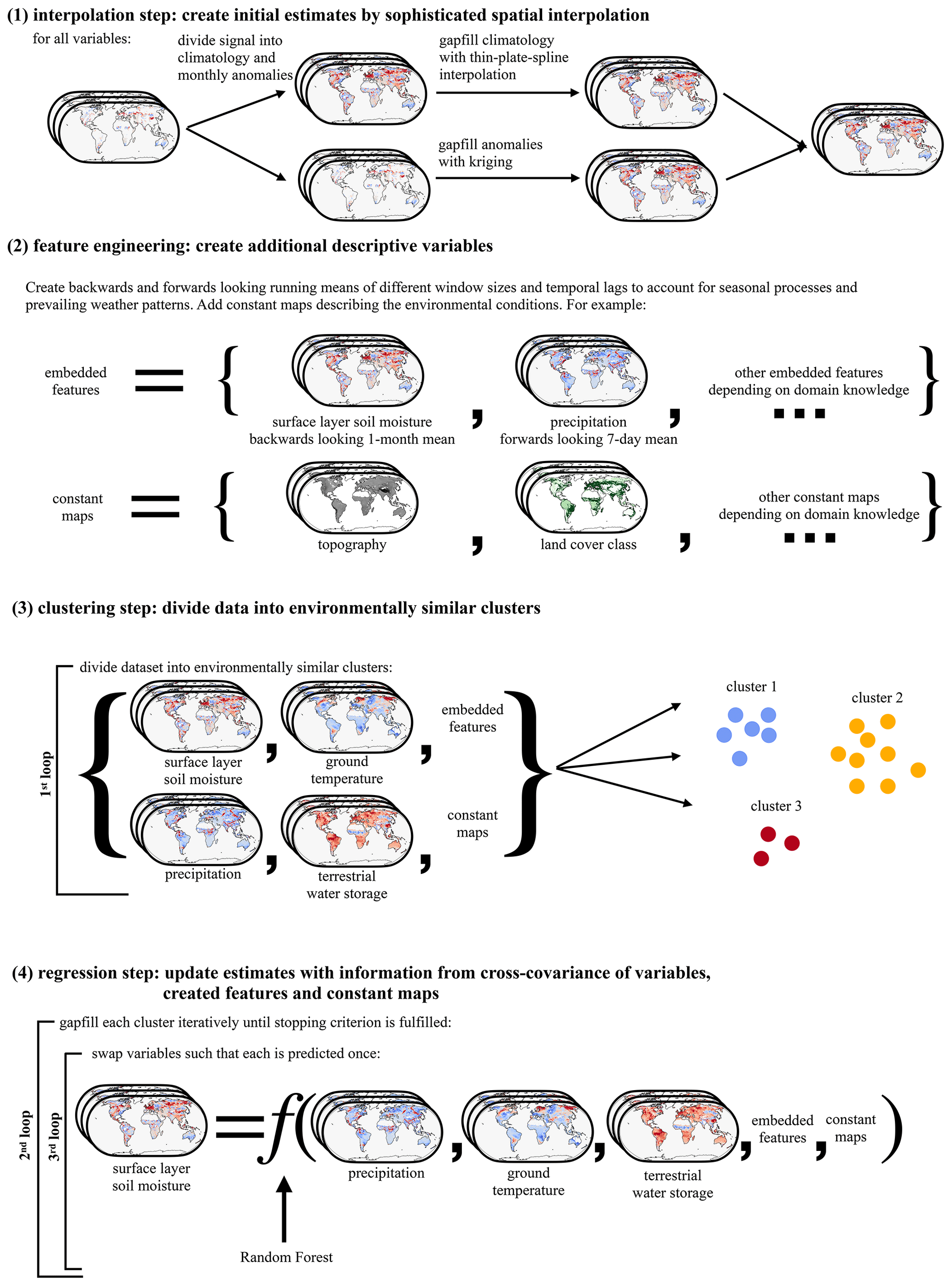
Figure 2Overview of the structure of the gap-filling framework. The framework is divided into four steps. In the first step (Sect. 2.1), any missing value is gap filled by an initial estimate from the spatiotemporal context. This step is called interpolation step. Here the spatiotemporal mean of observed values surrounding the missing value is used for each variable individually. In the second step (Sect. 2.2), embedded features are created to inform about time-dependent processes. In the third step, the data are divided into environmentally similar clusters (Sect. 2.3, Algorithm 1). In the fourth step (Sect. 2.4, Algorithm 1), the initial estimates from step 1 are updated while accounting for the dependence structure among all considered variables. This is achieved by first grouping available data points into environmentally similar clusters and then iteratively updating the initial estimates using a supervised learning algorithm.
We aim to develop a multivariate gap-filling framework that exploits the spatial, temporal, and cross-variable dependence structure of Earth system observations to produce estimates for missing values even if they are present in all variables. To achieve this goal we build upon geo-statistical interpolation and a multivariate gap-filling approach that has been popularized in other fields, namely the MissForest algorithm (van Buuren, 2018; Stekhoven and Bühlmann, 2012). In particular, we aim to utilize (1) spatial neighbourhood information, (2) temporal correlation, and (3) and statistical dependence across all considered variables. With these design requirements we aim to recover both the marginal distributions and the dependence among variables at any location with missing values. The CLIMFILL framework works mutually for all considered variables, meaning that information available in each of the variables is used for filling the gaps of all the other variables. With this design we implicitly assume that if one variable is not observed at a certain space–time point, a subset of the other variables might be observed and can reconstruct the missing value while conserving the dependence structure among all variables.
The framework is divided into four steps (Fig. 2). In the first step, initial estimates for all missing values are produced by spatial interpolation of each variable independently, i.e. in a univariate setting. In the second step, the data are pre-processed to account for spatial and temporal dependence, which contributes to approximate physical links among different variables. In the third step, the data are divided into environmentally similar clusters. In the fourth and final step, the multivariate dependencies are taken into account. The initial estimates from the interpolation step are updated using an iterative procedure that aims to reconstruct the dependence structure between the variables with the aim of increasing the accuracy of the initial estimates.
2.1 Step 1: interpolation for integrating spatial context
The interpolation step creates initial estimates based on the spatial or spatiotemporal context of the gap using interpolation. Following the approach of Haylock et al. (2008), the data are first divided into monthly climatology maps and anomalies. The climatology maps are gap filled using thin plate spline interpolation to represent the spatial trends in the data. Subsequently, the daily anomalies from the monthly climatology are gap filled using kriging. In contrast to the E-OBS dataset created in Haylock et al. (2008) from in situ observations, satellite data has a much larger number of observed values, making a direct implementation of this approach computationally infeasible. For the interpolation of the monthly climatology maps we therefore restrict the thin plate spline interpolation to the 50 closest neighbours of each point. The interpolation of the daily anomalies follows Das et al. (2018), who suggest reducing complexity of kriging and Gaussian process regression by repeated interpolations on random sub-samples of all available data points and averaging the resulting estimates. More specifically, the missing values in the anomalies are estimated by randomly selecting 1000 observed points per month over which the interpolation is calculated. This is repeated five times, and the mean of all interpolations for each missing point is taken as the gap fill estimate. As a consequence of these adaptations, the interpolation step becomes computationally feasible, but the uncertainty of the interpolation cannot be estimated. Finally, monthly maps and anomalies are summed up to form the initial gap fill estimate from step 1.
2.2 Step 2: feature engineering informed by process knowledge
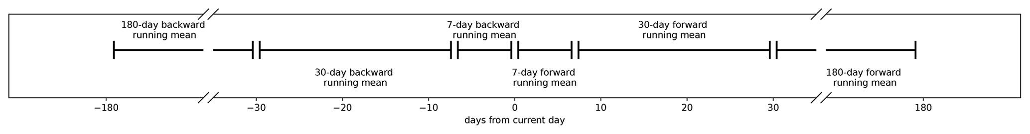
An important step in data-driven modelling is taking care that the data consist of informative variables that represent the mechanisms at work. This creation of variables or “features” guided by expert knowledge is called feature engineering. Earth observations often inform about time-dependent processes like seasonal effects, weather persistence, or soil moisture memory effects that act from daily to monthly or subseasonal timescales (Nicolai-Shaw et al., 2016). To account for such antecedent and subsequent effects, backward- and forward-looking running means of different window sizes and temporal lags are included. This is motivated by prior work on large-scale runoff estimation (Gudmundsson and Seneviratne, 2015). Given a variable at longitude i, latitude j, and time step t we define the window size s and time lag l over which a running mean of a variable v is computed:
resulting in an embedded feature v* produced from variable v. We create embedded features of 7 d (), 1-month (), and 6-month () backward and forward running means in such way that the windows are not overlapping (see Fig. 3). This way six additional features are created for each variable. Furthermore, gap-free time-independent maps describing properties of the land surface such as topography or land cover can be included. Maps of altitude, topographic complexity, land cover class, and land cover height from ERA-5, as well as latitude, longitude, and time, are added to the list of features and copied for each time step.
The above procedure thus results in a set of 35 features: the four variables and the six embedded features of each of the four variables (totalling 24 embedded features); the four maps; and latitude, longitude, and time information. All data are standardized to have zero mean and a standard deviation of 1. We perform feature selection experiments (see Sect. 2.2) to find the most descriptive subset of these 34 features, which we then use for computing the results.
2.3 Step 3: grouping the data into environmentally similar clusters
Depending on the climate regime and the season, different processes might govern the local dependence among variables. Furthermore, geoscientific datasets are very large, and the computational costs of supervised learning methods do often not scale linearly with the number of samples. We therefore split the data into K environmentally similar clusters (Algorithm 1, line 3) in which the multivariate gap filling happens (Algorithm 1, first loop, lines 4 to 16). This grouping is done in such way that grid points can be in different clusters at different time steps. For example, a grid point in the Mediterranean area can be in a different cluster in winter than in summer, accounting for seasonally varying climate phenomena such as changing soil moisture regimes (Seneviratne et al., 2010). Here a k-means algorithm is used, and the data are partitioned into 30 clusters. This value is chosen such that the number of data points per cluster is large enough to ensure that the regression model can be calibrated efficiently but not so small that no individual clusters consist of missing values entirely.
2.4 Step 4: optimizing the initial estimates by accounting for the dependence between variables
In the fourth step, the initial estimates from step 1 are updated by accounting for the dependence between variables. Within each of the clusters Xk, the algorithm repeatedly iterates over the variables until convergence is reached. This procedure builds upon the MissForest algorithm by Stekhoven and Bühlmann (2012). For each variable v, a random forest model (Breiman, 2001) is fitted to the cluster to predict originally missing values in all variables based on the remaining features. Random forests have favourable properties for gap-filling applications: they can handle mixed types of data, they are scalable to large amounts of data, and they are non-parametric, i.e. adaptive to linear and non-linear relationships (Tang and Ishwaran, 2017).
This core mechanism of CLIMFILL is detailed in the inner, third loop of Algorithm 1 (lines 6 to 14): the current variable is selected from the cluster as predictand . All other columns of Xk form the predictor table , where −v denotes the set of all variables and features except v. Subsequently, both and are divided into two sets of data points. (1) All data points where was originally observed are used to fit the supervised learning method , and (2) all data points where was missing are predicted from the fitted function to overwrite the former estimates, i.e. . Note that the training data most likely include originally missing values in the predictor variables. Here, the estimates from the interpolation step play the role of giving an initial estimate in the first iteration. Once the algorithm has iterated over all the variables, each missing value has been updated once. The algorithm is stopped (stopping criterion, Algorithm 1, second loop, lines 5 to 15) once the change in the estimates for the missing values is small between iterations (convergence) or a maximum number of iterations is reached (early stopping).
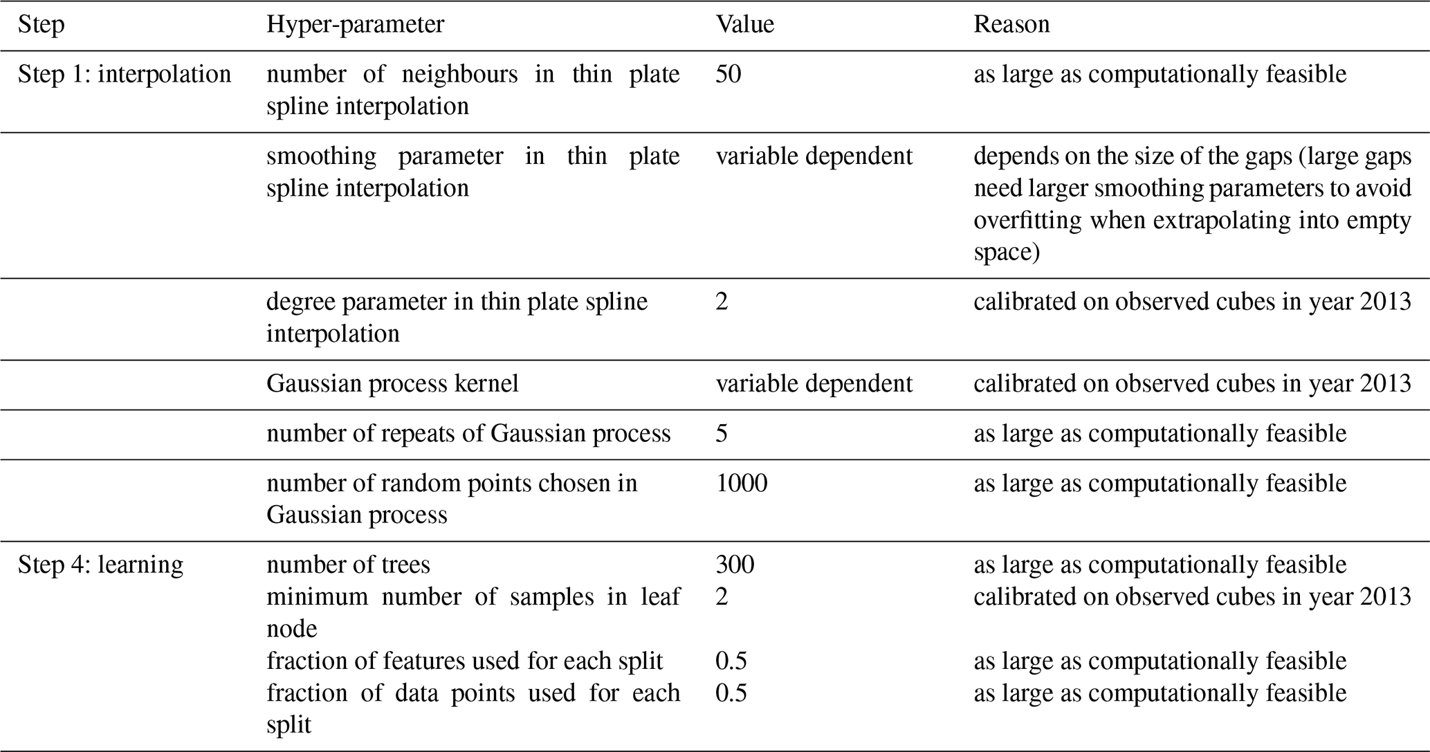
Note that the framework is set up such that each cluster learns different model parameters. With these choices the model is flexible to tailor its hyper-parameters individually to each variable and the regression parameters individually to each cluster. The hyper-parameters of the interpolation and the regression step are largely determined by computational limits of the available resources (for an overview, see Table A2). Where possible, we calibrated the remaining hyper-parameters by cutting out spatiotemporal cubes of observed data in year 2013 and compare values gap filled with CLIMFILL with the originally observed ones.
Algorithm 1Pseudo-code algorithm of the CLIMFILL clustering and learning step (steps 3 and 4), where K is the number of clusters, nv is the number of variables, and nf the number of features. X−v refers to the data table with all variables (columns) except v. Algorithm and pseudo-code are adapted from Stekhoven and Bühlmann (2012).
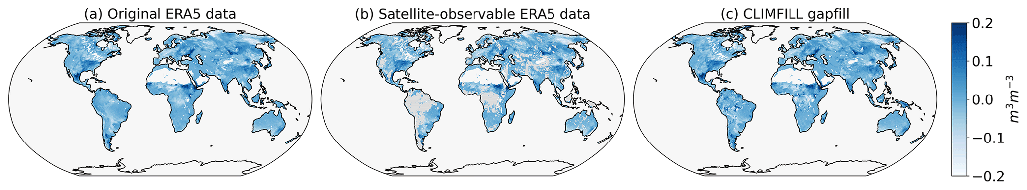
Figure 4Comparison of (a) the original naturally gap-free ERA-5 reanalysis, (b) the same data but where only satellite-observable values are shown, and (c) the gap-filled data created from CLIMFILL after starting with the gappy data in (b). The maps show an example snapshot of ERA-5 surface-layer soil moisture anomaly on 1 August 2020. CLIMFILL successfully reconstructs major anomalies in surface-layer soil moisture for this day. The anomalies are calculated by subtracting the monthly mean values.
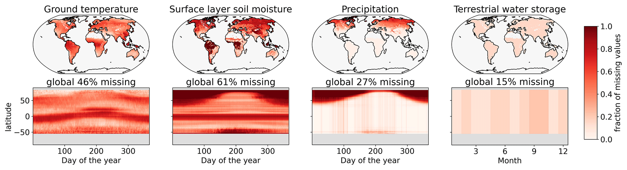
Figure 5Fraction of missing data regarding ground temperature from MODIS, ESA-CCI soil moisture, GPM precipitation, and GRACE terrestrial water storage observations in the years 2003–2020. The upper panels show the fraction of missing data per land point on the ERA-5 grid, and the lower panels show fraction of missing values per latitude and day of the year. The data are down-sampled to daily values, with the exception of GRACE, which has monthly resolution.
To illustrate the impact of fragmented observational records, we focus here on the study of land–climate dynamics. At the land–atmosphere boundary, a complex interplay between soil moisture, temperature, and precipitation governs much of the water and energy balance at the surface (Seneviratne et al., 2010). Thus, a combination of atmospheric and terrestrial processes influences local climate (Greve et al., 2014; Seneviratne et al., 2010), the development of hot and dry extreme events (Wehrli et al., 2019; Miralles et al., 2019; Mueller and Seneviratne, 2012), changes in freshwater availability (Gudmundsson et al., 2021), and the interaction of all these factors with climate change (Seneviratne et al., 2010). These interactions are inherently multivariate and act on different timescales, making it necessary to observe the variables at a fine spatial and temporal resolution. Consequently, the study of land–climate dynamics requires observations spanning several components of the Earth system, including the land water and energy balances and the atmospheric state.
Since the original values that need to be gap filled are unobserved, we fall back on naturally gap-free atmospheric reanalysis data for benchmarking the framework. We use land-only global reanalysis data from ERA-5 at 0.25∘ resolution for the years 2003–2020 (see Hersbach et al., 2020). ERA-5 is chosen as a gap-free dataset because of its advanced representation of land surface processes (Hersbach et al., 2020) and improved agreement of relevant surface variables with available observations (Martens et al., 2020; Tarek et al., 2020; Albergel et al., 2018). The missingness patterns of satellite observations in the same period are extracted, regridded to ERA-5 resolution, and applied to the corresponding ERA-5 variable. In other words, only the part of the ERA-5 data that would have been observable by satellite are retained. In this “perfect dataset approach”, the “true” values of the variables at the locations of the missing values are known and can be compared with the estimates of the gap-filling framework (see Fig. 4).
The hourly ERA-5 data are aggregated to daily resolution. The aggregation function for each variable is chosen to be consistent with the satellite products (e.g. daily sums for precipitation and daily average for soil moisture; see Table A1 in Appendix A). Since GRACE is only available in monthly resolution, we up-sample the data by linearly interpolating the monthly values to daily resolution. Permanently glaciated areas and deserts (defined as areas with less 50 mm average yearly precipitation in the years 2003–2012) are masked. We extract the missingness pattern from four satellite remote sensing datasets related to land–climate interactions and apply it to the ERA-5 dataset: ESA-CCI surface-layer soil moisture (Gruber et al., 2019; Dorigo et al., 2017; Gruber et al., 2017), MODIS ground temperature (Wan et al., 2015), GPM precipitation (Huffmann et al., 2019), and GRACE terrestrial water storage (Swenson, 2012; Landerer and Swenson, 2012; Swenson and Wahr, 2006). These variables represent central interactions between soil moisture and climate that drive land water and energy balance through the soil moisture–temperature and soil moisture–precipitation feedbacks (Seneviratne et al., 2010). Selecting both microwave remote sensing measurements of surface-layer soil moisture and total water storage of the land surface is a compromise that aims to include as much possible information about root zone soil moisture as is available via remote sensing.
There are ubiquitous missing values in the selected satellite observations (Fig. 5). Since the missingness patterns only partially overlap, the selected set of variables is a good candidate for mutual gap filling. Ground temperature is missing where there is cloud cover, with the maximum amount of missing values in the inner tropics and extratropical storm tracks and moving along latitudinal bands throughout the year. Almost half of the ground temperature values (46 %) are missing globally in the considered years. Surface-layer soil moisture is only observed in 39 % of all cases. It is missing where there is ice or snow cover or when vegetation is too dense. This is the most complicated missingness case because it exhibits the highest fraction of missing values and has considerable amount of land mass where high vegetation cover prevents retrieval at all times. For precipitation, around a quarter of the values are missing (27 %); this is only true at high latitudes during winter. In the GPM remote sensing precipitation dataset, values in the presence of surface snow or ice are masked because of poor sensor quality (Huffmann et al., 2019). In postprocessing, Huffmann et al. (2019) use a sophisticated Kalman smoother time interpolation to fill the gaps from the retrieval. From available metadata, we retrieved the originally missing maps to be able to quantify the added value of mutual gap filling for precipitation. Terrestrial water storage is missing if the global measurement is discarded due to instrument failure or during calibration missions (Landerer, 2021), leading to individual months being missing and 15 % of values being missing total.
The results section is structured as follows. Sect. 4.1 compares CLIMFILL with three different feature sets and the interpolation step (experiments A through D in Table 1). At the end of this section, we settle on a feature set of CLIMFILL for the rest of the results. In Sect. 4.2, the theoretical upper performance limits given the data described in Sect. 3 are examined using simpler, artificial missingness patterns and changing fractions of missing values (experiments D, E, and F in Table 1). Finally, in Sect. 4.3 CLIMFILL is run for the whole period (2003–2020) (experiment D) and its gap-filling results are compared to the original, gappy part of the data that is observable by satellite.
4.1 Benchmarking against univariate interpolation
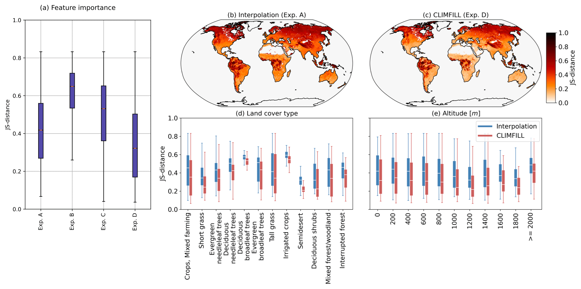
Figure 6Multivariate Jenson–Shannon (JS) distance for interpolation and CLIMFILL gap-filling processes. (a) Boxplots of JS distance between original the ERA-5 data and the interpolation, as well as all sets of features as described in Sect. 2.2. (b) Map of JS distance of univariate interpolation and (c) CLIMFILL considering the multivariate distribution of all variables. (d) JS distance per land cover type and (e) altitude for interpolation gap filling and CLIMFILL gap filling. Land cover type and altitude are extracted from ERA-5. Boxplots show the median as a white line, the box shows the upper and lower quartiles, and the whiskers are 1.5 times the quartile length over all land points with the specified land cover type or altitude.
Figure 7Bivariate and univariate histograms of surface-layer soil moisture and ground temperature in (a) the original ERA-5 data, (b) the subset of the original ERA-5 data that would have been observable by satellite, and (c) the data that has been gap filled via univariate interpolation and (d) via CLIMFILL gap filling. For bivariate distributions of other variable pairs, see Fig. A1 in Appendix A.
The objective of the CLIMFILL framework is not only to reconstruct variables separately but also to recover multivariate dependencies. In this first part of the results, we illustrate the improvement of the multivariate gap-filling framework CLIMFILL compared to the univariate interpolation that takes place in the first step of the framework (experiment A). With this analysis, we can quantify the added value of incorporating information from the other variables present, which happens in step 4 of the framework. Furthermore, within this section we examine which subset of features created in step 2 is most descriptive for the problem at hand. This is done to ensure an informed decision about the set of features is made that reflects their usefulness in the gap-filling process. We try three different sets of features: (1) only the four variables (experiment B), (2) the variables plus their embedded features as described in Sect. 2.2 (experiment C), and (3) all of the features created in step 2, including the constant features describing land properties (experiment D). The benchmarking process therefore quantifies the merit of CLIMFILL compared to univariate interpolation and explores the possible feature space for combinations that improve the results.
To allow for a quantitative assessment of the similarity of the multivariate distributions of observed and simulated variables, we apply a scalar measure of multivariate similarity. In this study, we use the Jenson–Shannon distance (JS distance) (Lin, 1991). This measure compares the distance between two multivariate distributions, where a value of zero means that both distributions are identical and a value of one indicates that the distributions are not overlapping. We apply the JS distance on four-dimensional histograms computed of the four variables using 50 bins for each variable.
Figure 6 shows the JS distance between the original ERA-5 data and the interpolation as well as the different feature sets. Overall, the JS-distance is lower for CLIMFILL than for interpolation globally (Fig. 6a) for experiment D. Including all variables shows the best results overall. For the rest of the paper we will therefore refer to experiment D when referring to CLIMFILL. Regionally, the largest improvement between CLIMFILL and the interpolation is in the tropical and subtropical regions (Fig. 6b, c), where the high fraction of missing values inhibits the performance of interpolation. Taking a closer look at the results by dividing the global map into types of vegetation and altitudes (Fig. 6d, e) shows that the JS distance improves from interpolation to CLIMFILL for all altitudes and all land cover types. This indicates an improvement regarding the multivariate features in CLIMFILL gap filling globally for a wide range of environmental conditions. Overall, CLIMFILL has a higher skill when reconstructing the multivariate dependence structure of the original ERA-5 data compared to univariate interpolation.
To illustrate the complex impacts of missing values and their alleviation in univariate and multivariate gap filling, Fig. 7 exemplary shows the bivariate distribution of surface-layer soil moisture and ground temperature globally for the whole time period (all other possible combinations of variables are shown in Fig. A1). The part of the data that is observable from space (Fig. 7b) shows a collapsed distribution and clearly fails to recover the original bivariate distribution. Results after univariate interpolation recover parts of the distributions. CLIMFILL further improves this and recovers the shape of the original distribution. Thus, it generally provides an improved estimate of the bivariate distribution of surface-layer soil moisture and ground temperature such that it is closest to the original ERA-5 data despite knowing only the satellite-observable points.
4.2 Data-constrained upper performance limits

Figure 8Comparison of artificial (a) random and (b) swath-only missingness and (c) missingness in the real data in an example snapshot of ERA-5 ground temperature from 1 August 2003. Random missingness was created by randomly sampling without replacement from the pool of all grid points on land at all time steps in the desired fraction of missing values. In the swath-only missingness data we create long ellipses centred around the Equator to simulate characteristic satellite swath missingness patterns. Note that the two missingness patterns are not exactly the same for each day and variable to allow for cross-variable learning.
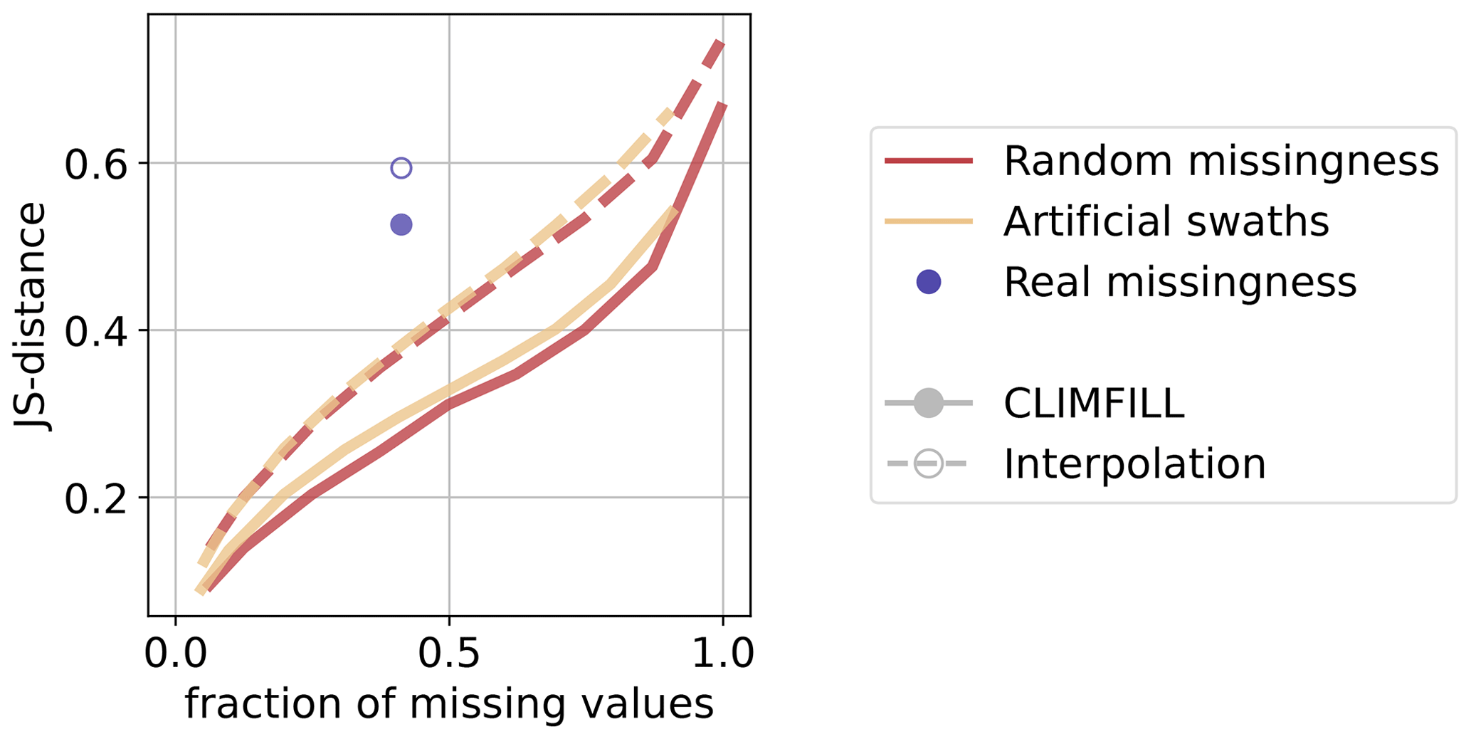
Figure 9Median performance of gap filling with CLIMFILL and univariate interpolation on different missingness patterns and fractions of missingness expressed in JS distance (for more details, see Sect. 4.2) per variable. Gap filling for random missingness and artificial swaths is executed for a range of fractions of missing values and is denoted as a line, while real missingness is only one case and is depicted as a point. The metrics are calculated over each time step for all non-satellite-observable values of grid points on land, and the median of all land points is also plotted.
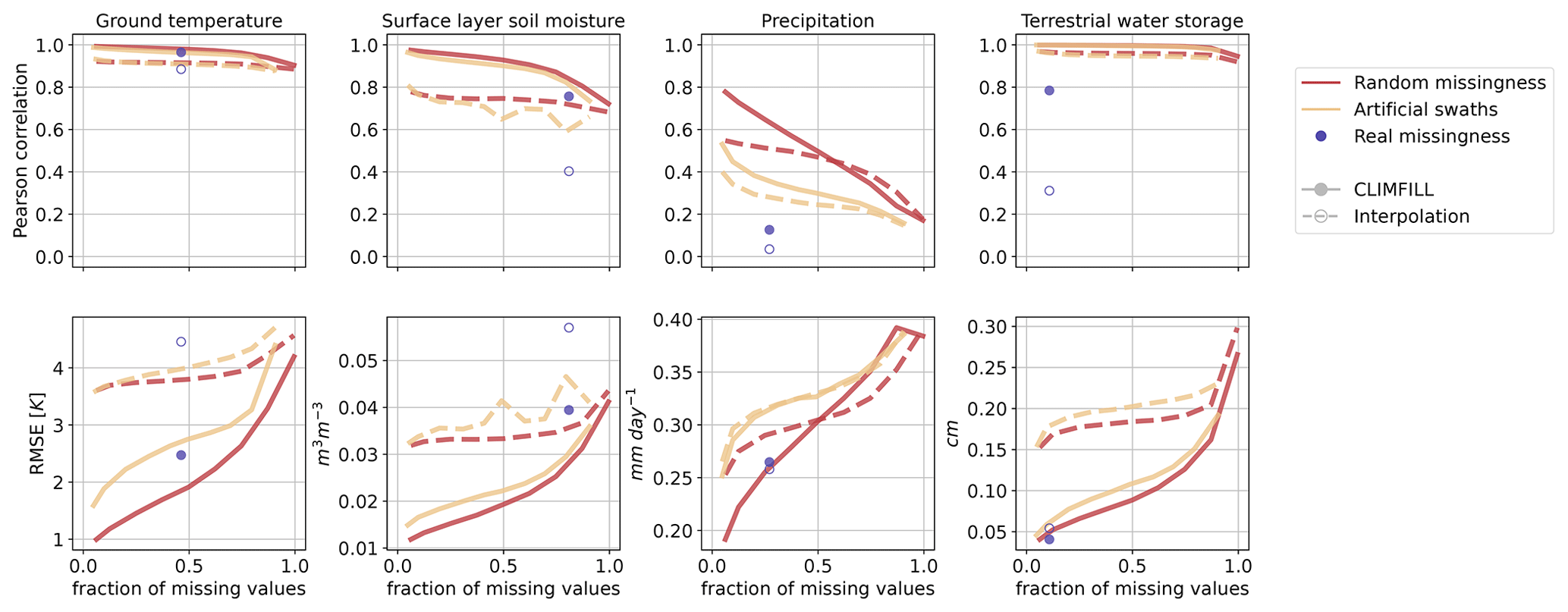
Figure 10Median performance of gap filling with CLIMFILL and univariate interpolation on different missingness patterns and fractions of missingness expressed by two metrics: Pearson correlation and root-mean-square error (RMSE) per variable. Gap filling for random missingness and artificial swaths is executed for a range of fractions of missing values and is denoted as a line, while real missingness is only one case that is depicted as point. The metrics are calculated over each time step for all non-satellite-observable values of grid points on land, and the median of all land points is also plotted.
Missing values in Earth observation data are often present in large proportions and in complex MNAR patterns. These characteristic properties of Earth observation data can hamper gap filling. We therefore are interested in exploring the envelope of data properties in which gap filling can be successful and seeing the deterioration of performance with increasing data sparsity and increasingly complex missing value patterns. In contrast to the last section, the goal is to show the upper limit of what is possible in gap filling with the complex missingness patterns exhibited by satellite observations. To this end, we rely on the four considered variables to test the impact of increasing fractions of missing data using idealized patterns. In particular, we delete (1) data according to a MCAR random missingness pattern (experiment E, Fig. 8a) and (2) by imitating satellite swaths, effectively creating MAR missingness patterns (experiment F, Fig. 8b). Both patterns are applied for fractions of missing values between 5 % and 95 % for each of the variables.
Multivariate JS distance (Fig. 9) and univariate statistical performance measures (Fig. 10) are used to compare original and gap-filled values for all performed experiments. With increasing fraction of missing values, the two artificial missingness cases increase in error, increase in their JS distance, and decrease in correlation. Once more than 80 % of the values are missing, the gap filling breaks down because not enough observed values are available for the iterative procedure to converge to a meaningful result. Random and artificial swath missingness show similar deterioration with increasing fraction of missing values, but values missing completely at random tend to be easier to estimate at all fractions of missing values. Gap filling random missingness is the easiest case, since it is likely that neighbouring or environmentally similar points are observed. MAR missingness exposes large patches of missing values, making spatiotemporal interpolation less effective and hence decreasing the gap-filling performance as compared to MCAR. Since the real (MNAR) missingness case is the most complex missingness pattern, these additional experiments serve as an upper limit on performance in the real case.
When moving from the artificial patterns of missingness to the real case (dots and circles in Figs. 9 and 10), the deterioration in performance is different for each of the variables. However, in most cases the metrics for the real missingness case are close to the artificial missingness patterns, suggesting CLIMFILL operates at the upper limit of what is possible with the complex missingness pattern of real observations. For ground temperature, a spatially and temporally smooth variable, the interpolation is already quite a good first guess, and its correlation is only slightly improved in CLIMFILL. However, the RMSE drops quite dramatically, indicating smaller biases in ground temperature for gap-filled data. In this case study, we found the biggest improvement compared to interpolation for surface-layer soil moisture despite its large fraction of missing values. This high performance could be due to the fact that surface-layer soil moisture exposes missingness in areas where other variables are observed, for example in the tropical forests, such that learning in this area is easier. Additionally, variable selection is centred around soil moisture, and soil moisture is a key variable of land hydrological processes. The most difficult case is precipitation. Precipitation estimates are only slightly improved with CLIMFILL compared to initial interpolation. Precipitation is influenced by several processes that are not captured within the four selected variables. For example, frontal rain patterns are mostly not explained by land surface properties but are governed by large-scale circulation. This is a challenging case and could still be further improved, for example by adding wind patterns to capture more synoptic features. Terrestrial water storage contains only a small fraction of missing values (15 %). Since the interpolation is only applied spatially, it fails for full months of missing data and therefore the difference in correlation between interpolation and CLIMFILL is particularly high.
4.3 Recovery of regional and local land–climate dynamics
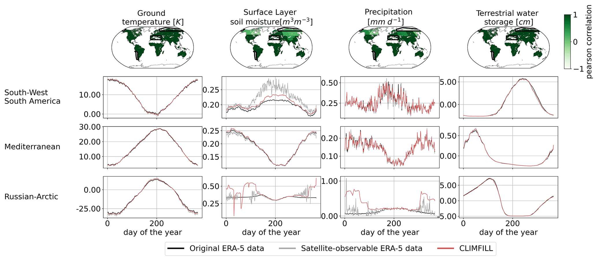
Figure 11Pearson correlation of regionally averaged mean seasonal cycles between CLIMFILL and the original ERA-5 data over IPCC reference regions (AR6 regions, Iturbide et al., 2020) (top row). Regionally averaged mean seasonal cycle of the physical values over selected regions in original ERA-5 data, satellite-observed ERA-5 data, and gap-filled CLIMFILL data (bottom three rows). The selected regions show the advantages and problems of each framework. For more information, see Sect. 4.3. For all other AR6 regions, see Fig. A2 in Appendix A.

Figure 12Pearson correlation of regionally averaged, deseasonalized monthly averages between CLIMFILL and the original ERA-5 data over IPCC reference regions (AR6 regions, Iturbide et al., 2020) (top row). Regionally averaged monthly averages of the physical values over selected regions in original ERA-5 data, satellite-observed ERA-5 data, and gap-filled CLIMFILL data (bottom three rows). The selected regions show the advantages and problems of each framework. For more information, see Sect. 4.3. For all other AR6 regions, see Fig. A5 in Appendix A.
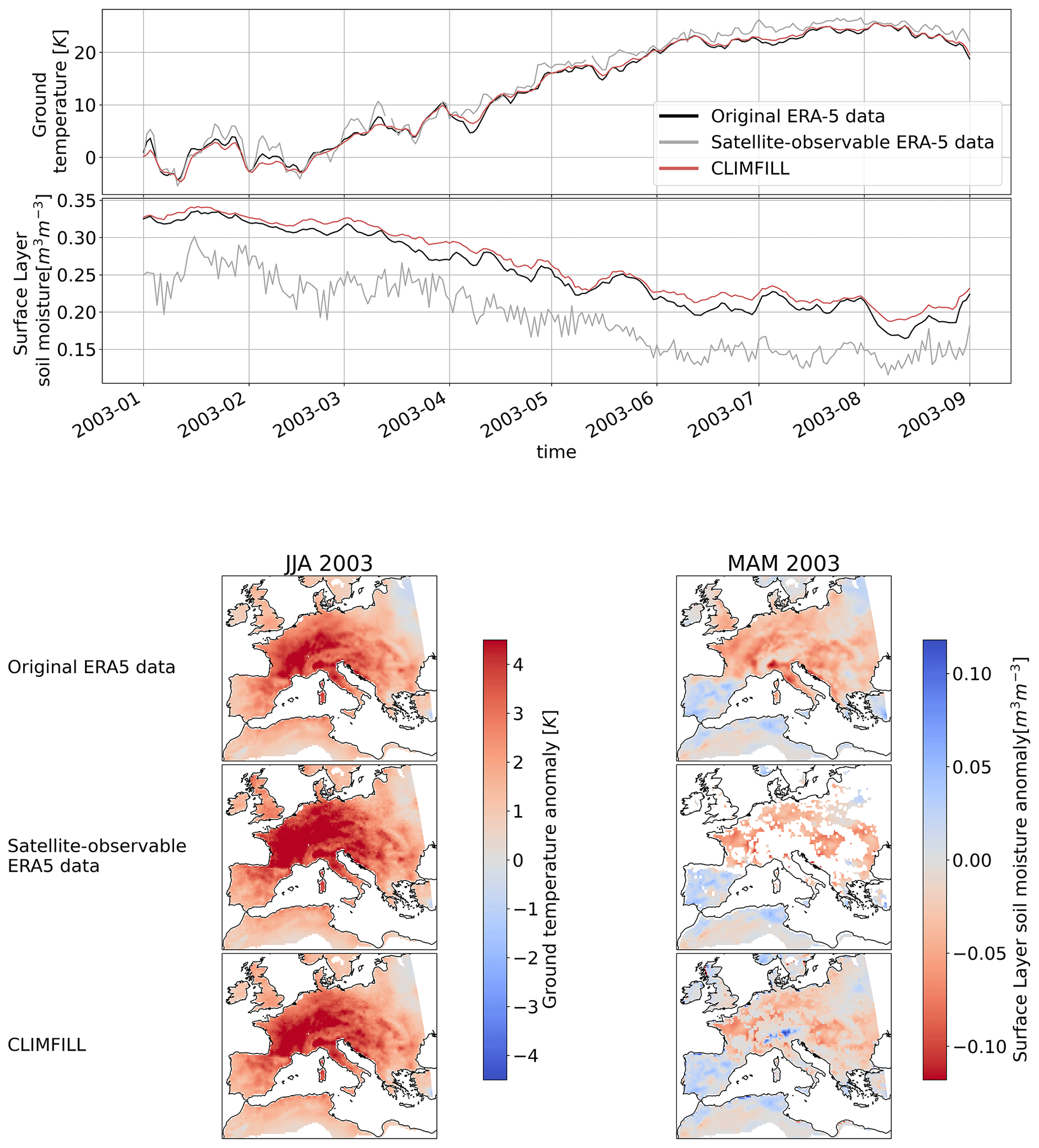
Figure 13Development of ground temperature and surface-layer soil moisture over central Europe from January to August 2003, depicting the European heatwave 2003 for ERA-5 original data, satellite-observable ERA-5-data and CLIMFILL gap fill. The maps show anomalies of ground temperature for the three cases in JJA 2003 and anomalies in surface-layer soil moisture in the 3 preceding months (MAM 2003) over Europe.
For any gap-filling framework to be useful for both scientific and practical applications it needs to be able to recover essential properties of the phenomena of interest. The coupling of energy and water between land and atmosphere at the land surface is a central, multivariate property of land–climate interactions that is currently underestimated in satellite data (Hirschi, 2014). By comparing CLIMFILL gap fill with the subset of data that can be observed from space, i.e. the gappy ERA-5 data (Fig. 4), we explore the role of missing values in this problem. This analysis is conducted over the whole available time period 2003–2020 (experiment D). More specifically, we show that leaving gaps in satellite data unfilled leads to biases and noise in estimates of regional and local climate feedbacks, and we also show how the CLIMFILL framework can contribute to overcoming this issue.
Figure 11 showcases the Pearson correlation between the mean seasonal cycle in original ERA-5 data and CLIMFILL estimates, as well as spatial averages of the variables for selected IPCC reference regions (AR6 regions; see Iturbide et al., 2020). Overall, we find good agreement between them for the majority of regions in the world. The missing values in the satellite-observable ERA-5 data result in a noisy signal and biased values in regional estimates from the satellite-observable data. CLIMFILL alleviates the noise, reduces the bias, and has a high correlation to original ERA-5 data for a majority of regions (for all other regions, see Fig. A2 in Appendix A). However, surface-layer soil moisture and precipitation suffer from gap-filling artefacts in high-latitude regions.
In Fig. 12, the reconstruction of month-to-month variability by CLIMFILL is shown. Monthly, deseasonalized anomalies of the four variables for years 2003–2020 are plotted as spatial averages for selected IPCC reference regions (for all other regions, see Fig. A5 in Appendix A). CLIMFILL is able to reconstruct the overall variability throughout the years. Here the skill for surface-layer soil moisture and precipitation estimates is again region dependent. High-latitude regions show decreased correlation compared to other regions and unrealistic values in winter.
There are multiple reasons for the unrealistic performance of CLIMFILL in high-latitude regions in winter. Firstly, precipitation gap filling is a challenging case due to its non-normal distribution. Secondly, soil moisture of frozen soil is hard to define. Thirdly, both variables suffer from unrealistic estimates of the interpolation step. These estimates that are created when the thin plate spline interpolation interpolates over areas where observed values are sparse and geographically far away, for example in the Russian Arctic during winter. These unrealistic values cannot be fully dampened by the iterative procedure in step 4 of CLIMFILL. Furthermore, precipitation is a challenging case due to its non-normal distribution. In future versions of the framework, a way to reduce this problem would be to not allow thin plate spline interpolation to estimate missing values that are too distant from observations, and instead rely on regional averages as an initial guess. In summary, for most variables in most regions CLIMFILL shows high correlation with the original values and reduces the bias and noise of estimates compared to only satellite-observable data for both the seasonal cycle and interannual variability, with some difficulties arising from the missingness patterns of surface-layer soil moisture and precipitation in high-latitude regions.
Soil moisture–temperature coupling plays an important role in the development of heat extremes (Wehrli et al., 2019; Vogel et al., 2017; Seneviratne et al., 2010). As a last measure, we look at the case study of the European 2003 heatwave. Figure 13 shows the regionally averaged development of ground temperature and surface-layer soil moisture for the first 8 months of 2003, as well as anomaly maps of ground temperature for JJA 2003 and surface-layer soil moisture for MAM 2003 for the three cases. With satellite-observable data only, the ground temperature is overestimated because only clear-sky values are reported and ground temperature values below clouds, usually systematically lower during daytime in summer, are missing. CLIMFILL alleviates this bias and brings absolute temperatures and anomalies close to the original ERA-5 data. A strong dry soil moisture anomaly in spring was characteristic for the 2003 heat event, which is overestimated and noisy in the satellite-observable data. CLIMFILL is able to recover the spatial distribution of the event and reduce the bias. The 2003 heatwave case showcases how CLIMFILL can alleviate biases and noise and show a more realistic heat extreme development compared to gappy satellite data.
Gaps in remotely sensed Earth observations are ubiquitous and unavoidable and lead to a fragmented record of observational data. Ignoring these gaps creates noisy and biased derived statistics and regional averages. Spatial univariate interpolations with state-of-the-art methods typically only consider one variable at a time and can therefore not fully recover the multivariate dependence structure between the variables. To bridge this gap, a framework for gap filling multivariate gridded Earth observations, CLIMFILL, is proposed. CLIMFILL estimates missing values by considering not only spatial and temporal factors but also multivariate dependence across variables. In doing so, CLIMFILL mines the highly structured nature of geoscientific datasets and combines interpolation-centred approaches common to geosciences and multivariate gap-filling methods from statistical literature. In contrast to popular upscaling approaches, CLIMFILL does not need a gap-free gridded “donor” variable for estimating missing values. Thus, the algorithm can digest complex patterns of missingness in multivariate Earth observations. CLIMFILL fills gaps in fragmented Earth observations while recovering the physical dependence structure among the considered variables. To this end, the CLIMFILL framework contributes to decreasing the inherent fragmentation of Earth observations, enables usage of multiple gappy satellite observations simultaneously, and is a helpful tool when working towards a coherent digital representation of the Earth.
This study illustrates the need for gap-filling approaches and the merit of CLIMFILL with a set of variables relevant for the study of land–climate dynamics. CLIMFILL is benchmarked in an exemplary setting of reanalysis data with a focus on variables relevant for the study of land–climate dynamics. To this end, reanalysis data have been deleted to match missing values in satellite observations in a “perfect dataset approach”. The multivariate JS distance shows that CLIMFILL recovers the dependence structure in the considered variables. Furthermore, univariate metrics show that CLIMFILL estimates have better agreement with original ERA-5 data compared to gappy data for many variables and regions. In summary, CLIMFILL is able to recover the dependence structure among several variables, in contrast to results obtained when missing values are not gap filled.
Although in this case study only four variables are considered, all of which are high in their respective fraction of missing values (up to more than two-thirds of the values missing) and complex in their pattern of missing values (always missing not at random), the multivariate gap filling with CLIMFILL improves estimates compared to univariate spatial interpolation. This is likely explained by the high correlation among the variables, which can to some degree counteract the complex missingness. This highlights that information from other available physically relevant variables can be beneficial for gap filling, indicating that the power of the framework might increase if even more dependent variables are included. Idealized experiments with simpler missingness patterns and different fractions of missing values within these four variables show that CLIMFILL improves upon univariate interpolation in all cases for all considered metrics, and the performance is close to easier cases with less complex missingness patterns for most variables.
In short, we have presented CLIMFILL, a multivariate gap-filling framework that exploits spatial, temporal, and multivariate information to create estimates for missing values in Earth observations. The fidelity of the framework has been successfully demonstrated in a case study centred around remote sensing observations relevant for the study of land–climate dynamics, which highlighted the merits of the approach compared to univariate interpolation. It is nevertheless important to stress that the “perfect dataset” approach employed here for benchmarking might not be fully representative for real observations. Therefore, we stress that the fidelity of the suggested algorithm has to be evaluated for real satellite observations and new applications. A natural next step could be to apply this gap-filling mechanism to a larger number of relevant observed variables and create a consistent, gap-free reconstruction of land hydrology.
Missing values in Earth observations are ubiquitous. Our efforts should centre around reducing these gaps in observations by, e.g. enhancing sensors, developing new measurement techniques, or closing gaps in observational networks. Looking at the problem from the other end, another approach could be to optimize the current observational capacities for information completeness, for example utilizing methods from information theory (Bauer et al., 2021a) and first tackle the gaps that are the largest or most severe for data analysis (both in natural and physical space). However, missing values will still remain unavoidable in many observations. Where they are present, it is imperative to develop dependable estimates that also consider links among variables. To this end, the CLIMFILL framework is developed to not only produce dependable estimates of individual variables but also to recover multivariate dependencies, eventually facilitating the creation of gap-free observational data products for environmental monitoring that also enable the study of Earth system processes, allow observation-only process analysis, or help to assimilate relevant but gappy observations into physical models.
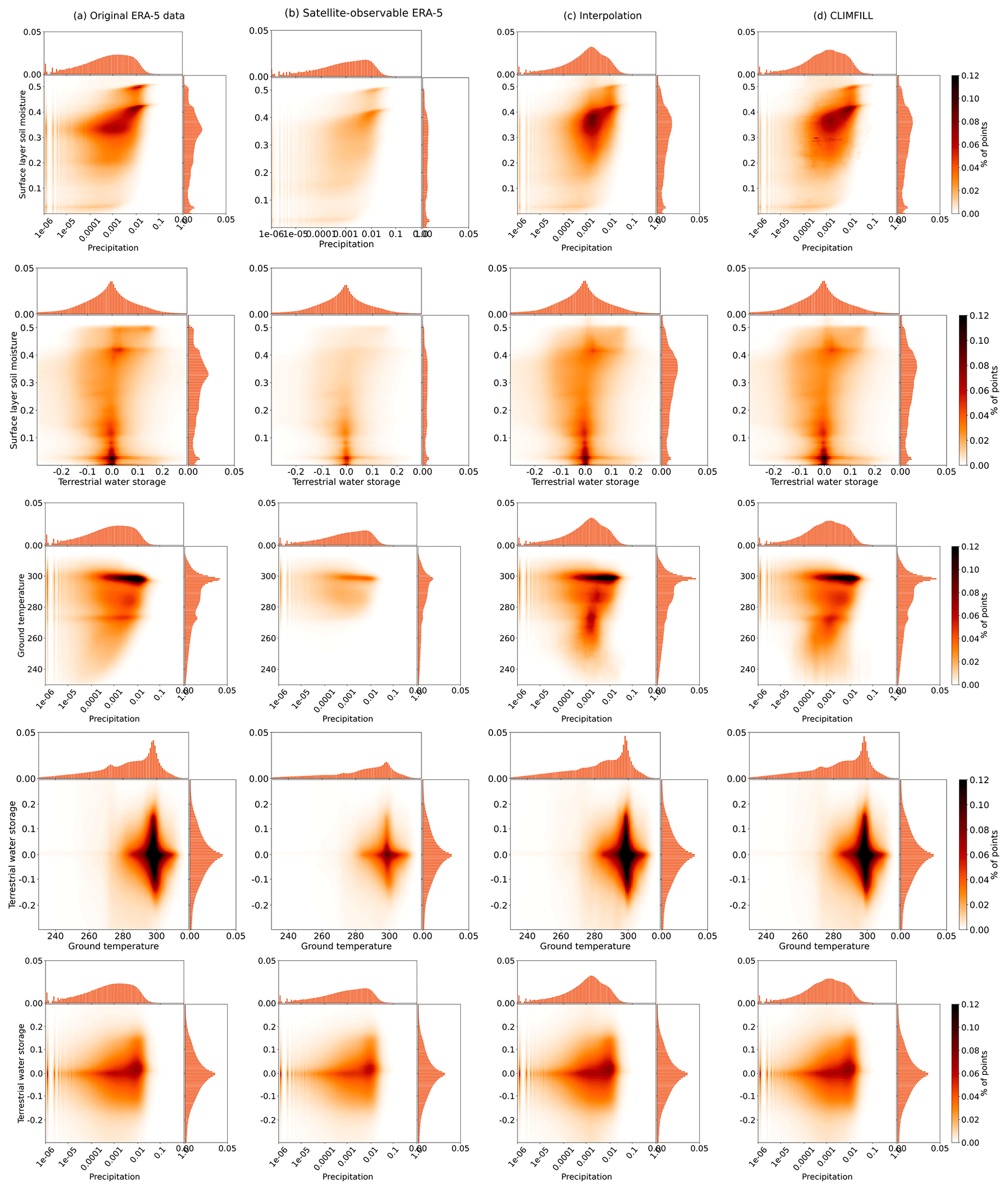
Figure A1Improvement of multivariate distribution with CLIMFILL gap filling: 2D histogram for all other combinations of variables (apart from the one already shown in Fig. 7) for the original ERA-5 data, satellite-observable ERA-5 data, the interpolation gap-filled data and CLIMFILL gap-filled data.

Figure A2Mean seasonal cycle over all IPCC reference regions on land except Antarctica (AR6 regions, as described in Iturbide et al., 2020) for the original ERA-5 data, satellite-observed ERA-5 data, and data gap filled with CLIMFILL.
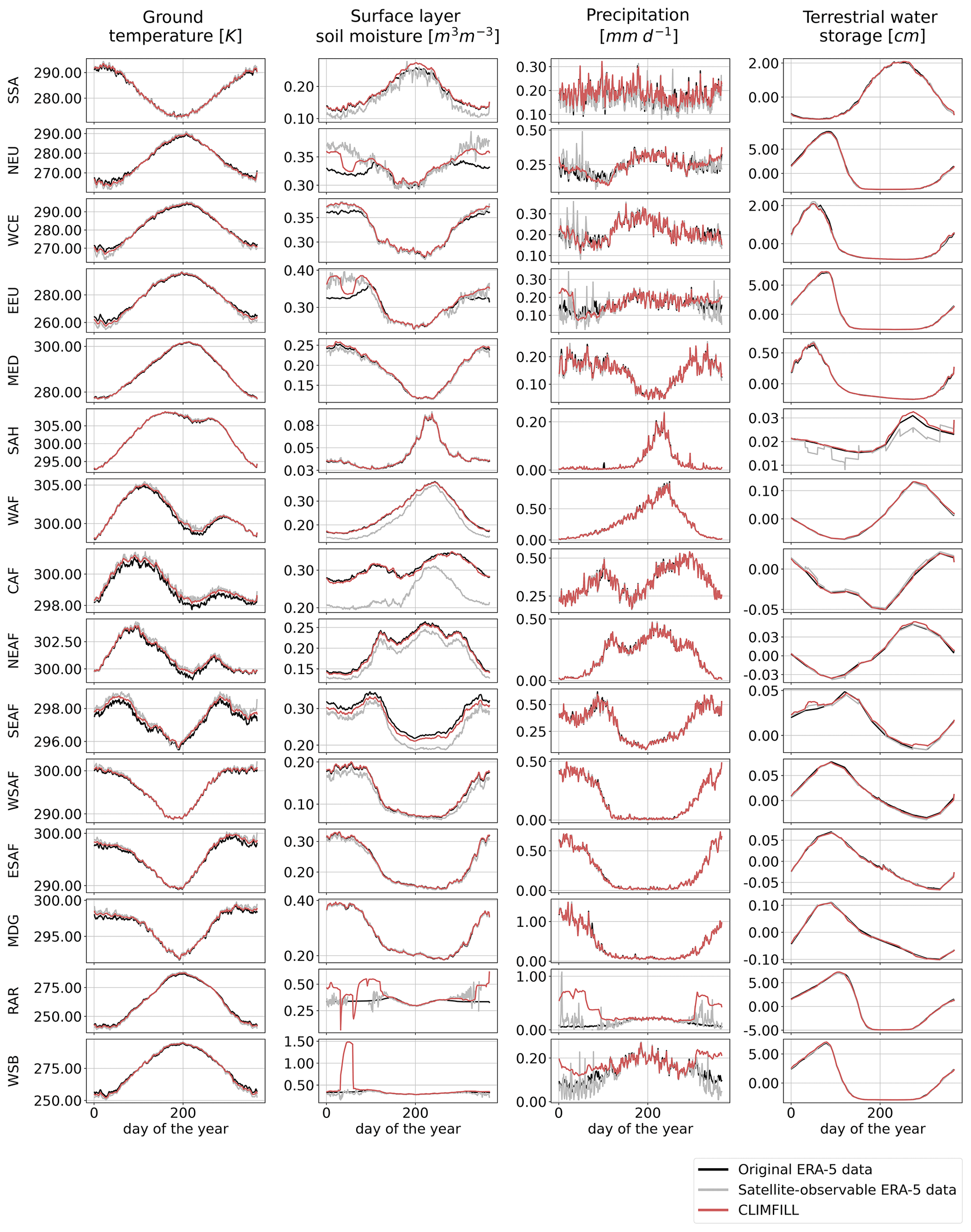

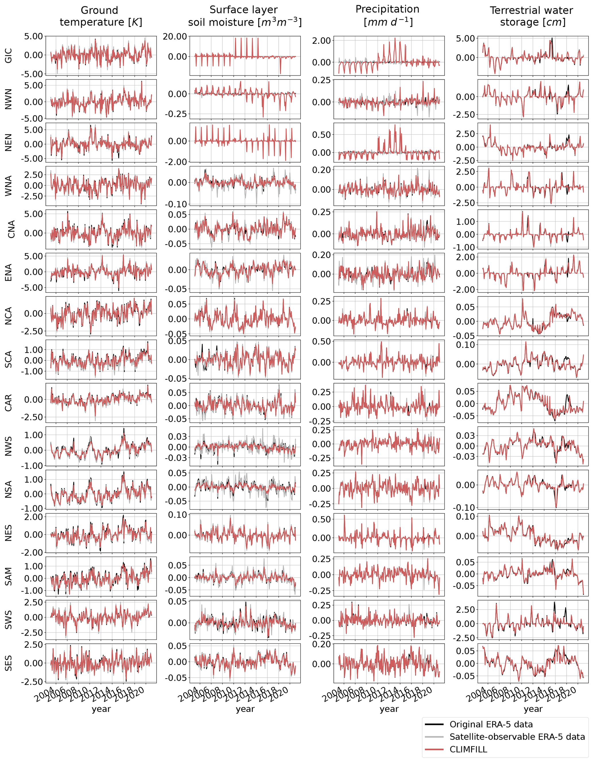
Figure A5Interannual variability over all IPCC reference regions on land except Antarctica (AR6 regions, as described in Iturbide et al., 2020) for the original ERA-5 data, satellite-observed ERA-5 data, and data gap filled with CLIMFILL.

Table A1Mapping of ERA-5 variables (in bold) with satellite observations.

Table A2Hyper-parameters of each step, their respective values, and how they were determined.
The current version of CLIMFILL is available from the project website (https://github.com/climachine/climfill, last access: 7 June 2022) under the Apache 2.0 License. The exact version of the model used to produce the results used in this paper is archived on Zenodo (https://doi.org/10.5281/zenodo.4773663, Bessenbacher et al., 2021), as are scripts to run the model and produce the plots for all the simulations presented in this paper. CLIMFILL was written in Python (Python Software Foundation, https://www.python.org/, last access: 7 June 2022) with core packages including xarray (Hoyer et al., 2020), NumPy (Harris et al., 2020), Matplotlib (Hunter, 2007), scikit-learn (Pedregosa et al., 2011), regionmask (Hauser, 2021), and scipy (Virtanen et al., 2020). The used ERA-5 data are publicly available at https://www.ecmwf.int/en/forecasts/datasets/reanalysis-datasets/era5 (last access: 16 February 2021).
VB, LG, and SIS designed the study based on an initial idea from LG. VB and LG developed the framework and the evaluation. VB carried out the analysis and drafted the text. All authors contributed to reviewing and editing the article.
The contact author has declared that neither they nor their co-authors have any competing interests.
Publisher's note: Copernicus Publications remains neutral with regard to jurisdictional claims in published maps and institutional affiliations.
The authors would like to thank Nicolai Meinshausen for input on the initial idea, Mathias Hauser for help in publishing the accompanying Python package, and Martin Hirschi for post-processing the ERA-5 data. Some of the calculations were performed using the Euler cluster at ETH Zurich. We would like to thank the ECMWF for creating and providing the ERA-5 reanalysis product. We would like to thank Johannes Senn, Joel Zeder, Jonas Jucker, and Roberto Villalobos for feedback on the draft. Lastly, we thank the reviewers for their very useful feedback, which greatly helped to improve this study.
This research has been supported by the Eidgenössische Technische Hochschule Zürich (grant no. ETH-08 19-1) and the European Space Agency (grant no. 4000126684/19/I-NB).
This paper was edited by Tomomichi Kato and reviewed by Rene Orth and two anonymous referees.
Albergel, C., Dutra, E., Munier, S., Calvet, J.-C., Munoz-Sabater, J., de Rosnay, P., and Balsamo, G.: ERA-5 and ERA-Interim driven ISBA land surface model simulations: which one performs better?, Hydrol. Earth Syst. Sci., 22, 3515–3532, https://doi.org/10.5194/hess-22-3515-2018, 2018. a
Alemohammad, S. H., Fang, B., Konings, A. G., Aires, F., Green, J. K., Kolassa, J., Miralles, D., Prigent, C., and Gentine, P.: Water, Energy, and Carbon with Artificial Neural Networks (WECANN): a statistically based estimate of global surface turbulent fluxes and gross primary productivity using solar-induced fluorescence, Biogeosciences, 14, 4101–4124, https://doi.org/10.5194/bg-14-4101-2017, 2017. a
Balsamo, G., Agusti-Panareda, A., Albergel, C., Arduini, G., Beljaars, A., Bidlot, J., Blyth, E., Bousserez, N., Boussetta, S., Brown, A., Buizza, R., Buontempo, C., Chevallier, F., Choulga, M., Cloke, H., Cronin, M. F., Dahoui, M., De Rosnay, P., Dirmeyer, P. A., Drusch, M., Dutra, E., Ek, M. B., Gentine, P., Hewitt, H., Keeley, S. P., Kerr, Y., Kumar, S., Lupu, C., Mahfouf, J.-F., McNorton, J., Mecklenburg, S., Mogensen, K., Muñoz-Sabater, J., Orth, R., Rabier, F., Reichle, R., Ruston, B., Pappenberger, F., Sandu, I., Seneviratne, S. I., Tietsche, S., Trigo, I. F., Uijlenhoet, R., Wedi, N., Woolway, R. I., and Zeng, X.: Satellite and In Situ Observations for Advancing Global Earth Surface Modelling: A Review, Remote Sens., 10, 2038, https://doi.org/10.3390/rs10122038, 2018. a, b
Banerjee, S., Gelfand, A. E., Finley, A. O., and Sang, H.: Gaussian predictive process models for large spatial data sets, J. Roy. Stat. Soc.-B, 70, 825–848, https://doi.org/10.1111/j.1467-9868.2008.00663.x, 2008. a
Bauer, P., Thorpe, A., and Brunet, G.: The quiet revolution of numerical weather prediction, Nature, 525, 47–55, https://doi.org/10.1038/nature14956, 2015. a
Bauer, P., Dueben, P. D., Hoefler, T., Quintino, T., Schulthess, T. C., and Wedi, N. P.: The digital revolution of Earth-system science, Nature Computational Science, 1, 104–113, https://doi.org/10.1038/s43588-021-00023-0, 2021a. a
Bauer, P., Stevens, B., and Hazeleger, W.: A digital twin of Earth for the green transition, Nat. Clim. Change, 11, 80–83, https://doi.org/10.1038/s41558-021-00986-y, 2021b. a, b
Bessenbacher, V., Seneviratne, S. I., and Gudmundsson, L.: CLIMFILL (v0.9), Zenodo [code], https://doi.org/10.5281/zenodo.6475578, 2021. a
Bhattacharjee, S. and Chen, J.: Prediction of Satellite-Based Column CO2 Concentration by Combining Emission Inventory and LULC Information, IEEE T. Geosci. Remote, 58, 8285–8300, https://doi.org/10.1109/TGRS.2020.2985047, 2020. a
Bocquet, M., Brajard, J., Carrassi, A., and Bertino, L.: Data assimilation as a learning tool to infer ordinary differential equation representations of dynamical models, Nonlinear Proc. Geoph., 26, 143–162, https://doi.org/10.5194/npg-26-143-2019, 2019. a
Breiman, L.: Random Forests, Mach. Learn., 45, 5–32, https://doi.org/10.1023/A:1010933404324, 2001. a
Brocca, L., Ciabatta, L., Massari, C., Moramarco, T., Hahn, S., Hasenauer, S., Kidd, R., Dorigo, W., Wagner, W., and Levizzani, V.: Soil as a natural rain gauge: Estimating global rainfall from satellite soil moisture data, J. Geophys. Res.-Atmos., 119, 5128–5141, https://doi.org/10.1002/2014JD021489, 2014. a, b
Brooks, E. B., Thomas, V. A., Wynne, R. H., and Coulston, J. W.: Fitting the Multitemporal Curve: A Fourier Series Approach to the Missing Data Problem in Remote Sensing Analysis, IEEE T. Geosci. Remote, 50, 3340–3353, https://doi.org/10.1109/TGRS.2012.2183137, 2012. a, b
Chiles, J.-P. and Delfiner, P.: Geostatistics: modeling spatial uncertainty, Wiley series in probability and statistics, Wiley, Hoboken, N. J., 2nd edn., ISBN 9780470183151, 2012. a
Cowtan, K. and Way, R. G.: Coverage bias in the HadCRUT4 temperature series and its impact on recent temperature trends, Q. J. Roy. Meteor. Soc., 140, 1935–1944, https://doi.org/10.1002/qj.2297, 2014. a, b, c
Cressie, N. and Wikle, C. K.: Statistics for spatio-temporal data, John Wiley & Sons, ISBN 0471692743, 2015. a
Cressie, N., Frey, J., Harch, B., and Smith, M.: Spatial prediction on a river network, J. Agr. Biol. Envir. St., 11, 127–150, https://doi.org/10.1198/108571106X110649, 2006. a, b
Das, S., Roy, S., and Sambasivan, R.: Fast Gaussian Process Regression for Big Data, Big Data Research, 14, 12–26, https://doi.org/10.1016/j.bdr.2018.06.002, 2018. a, b
Datta, A., Banerjee, S., Finley, A. O., and Gelfand, A. E.: Hierarchical Nearest-Neighbor Gaussian Process Models for Large Geostatistical Datasets, J. Am. Stat. Assoc., 111, 800–812, https://doi.org/10.1080/01621459.2015.1044091, 2016. a
Davenport, M. A. and Romberg, J.: An Overview of Low-Rank Matrix Recovery From Incomplete Observations, IEEE J. Sel. Top. Signa., 10, 608–622, https://doi.org/10.1109/JSTSP.2016.2539100, 2016. a
Dee, D. P., Uppala, S. M., Simmons, A. J., Berrisford, P., Poli, P., Kobayashi, S., Andrae, U., Balmaseda, M. A., Balsamo, G., Bauer, P., Bechtold, P., Beljaars, A. C. M., van de Berg, L., Bidlot, J., Bormann, N., Delsol, C., Dragani, R., Fuentes, M., Geer, A. J., Haimberger, L., Healy, S. B., Hersbach, H., Hólm, E. V., Isaksen, L., Kållberg, P., Köhler, M., Matricardi, M., McNally, A. P., Monge-Sanz, B. M., Morcrette, J.-J., Park, B.-K., Peubey, C., de Rosnay, P., Tavolato, C., Thépaut, J.-N., and Vitart, F.: The ERA-Interim reanalysis: configuration and performance of the data assimilation system, Q. J. Roy. Meteor. Soc., 137, 553–597, https://doi.org/10.1002/qj.828, 2011. a
de Jeu, R. A. M., Wagner, W., Holmes, T. R. H., Dolman, A. J., van de Giesen, N. C., and Friesen, J.: Global Soil Moisture Patterns Observed by Space Borne Microwave Radiometers and Scatterometers, Surv. Geophys., 29, 399–420, https://doi.org/10.1007/s10712-008-9044-0, 2008. a
Dorigo, W., Wagner, W., Albergel, C., Albrecht, F., Balsamo, G., Brocca, L., Chung, D., Ertl, M., Forkel, M., Gruber, A., Haas, E., Hamer, P. D., Hirschi, M., Ikonen, J., de Jeu, R., Kidd, R., Lahoz, W., Liu, Y. Y., Miralles, D., Mistelbauer, T., Nicolai-Shaw, N., Parinussa, R., Pratola, C., Reimer, C., van der Schalie, R., Seneviratne, S. I., Smolander, T., and Lecomte, P.: ESA CCI Soil Moisture for improved Earth system understanding: State-of-the art and future directions, Remote Sens. Environ., 203, 185–215, https://doi.org/10.1016/j.rse.2017.07.001, 2017. a, b, c
Gelaro, R., McCarty, W., Suárez, M. J., Todling, R., Molod, A., Takacs, L., Randles, C. A., Darmenov, A., Bosilovich, M. G., Reichle, R., Wargan, K., Coy, L., Cullather, R., Draper, C., Akella, S., Buchard, V., Conaty, A., da Silva, A. M., Gu, W., Kim, G.-K., Koster, R., Lucchesi, R., Merkova, D., Nielsen, J. E., Partyka, G., Pawson, S., Putman, W., Rienecker, M., Schubert, S. D., Sienkiewicz, M., and Zhao, B.: The Modern-Era Retrospective Analysis for Research and Applications, Version 2 (MERRA-2), J. Climate, 30, 5419–5454, https://doi.org/10.1175/JCLI-D-16-0758.1, 2017. a
Gelfand, A. E. and Schliep, E. M.: Spatial statistics and Gaussian processes: A beautiful marriage, Spat. Stat., 18, 86–104, https://doi.org/10.1016/j.spasta.2016.03.006, 2016. a
Gerber, F., Jong, R. d., Schaepman, M. E., Schaepman-Strub, G., and Furrer, R.: Predicting Missing Values in Spatio-Temporal Remote Sensing Data, IEEE T. Geosci. Remote, 56, 2841–2853, https://doi.org/10.1109/TGRS.2017.2785240, 2018. a
Ghahramani, Z. and Jordan, M. I.: Learning from Incomplete Data, Tech. rep., Defense Technical Information Center, https://doi.org/10.21236/ADA295618, 1994. a
Ghiggi, G., Humphrey, V., Seneviratne, S. I., and Gudmundsson, L.: GRUN: an observation-based global gridded runoff dataset from 1902 to 2014, Earth Syst. Sci. Data, 11, 1655–1674, https://doi.org/10.5194/essd-11-1655-2019, 2019. a, b
Gramacy, R. B. and Apley, D. W.: Local Gaussian Process Approximation for Large Computer Experiments, J. Comput. Graph. Stat., 24, 561–578, https://doi.org/10.1080/10618600.2014.914442, 2015. a
Greve, P., Orlowsky, B., Mueller, B., Sheffield, J., Reichstein, M., and Seneviratne, S. I.: Global assessment of trends in wetting and drying over land, Nat. Geosci., 7, 716–721, https://doi.org/10.1038/ngeo2247, 2014. a
Gruber, A., Dorigo, W. A., Crow, W., and Wagner, W.: Triple Collocation-Based Merging of Satellite Soil Moisture Retrievals, IEEE T. Geosci. Remote, 55, 6780–6792, https://doi.org/10.1109/TGRS.2017.2734070, 2017. a
Gruber, A., Scanlon, T., van der Schalie, R., Wagner, W., and Dorigo, W.: Evolution of the ESA CCI Soil Moisture climate data records and their underlying merging methodology, Earth Syst. Sci. Data, 11, 717–739, https://doi.org/10.5194/essd-11-717-2019, 2019. a
Gudmundsson, L. and Seneviratne, S. I.: Towards observation-based gridded runoff estimates for Europe, Hydrol. Earth Syst. Sci., 19, 2859–2879, https://doi.org/10.5194/hess-19-2859-2015, 2015. a, b, c
Gudmundsson, L., Boulange, J., Do, H. X., Gosling, S. N., Grillakis, M. G., Koutroulis, A. G., Leonard, M., Liu, J., Müller Schmied, H., Papadimitriou, L., Pokhrel, Y., Seneviratne, S. I., Satoh, Y., Thiery, W., Westra, S., Zhang, X., and Zhao, F.: Globally observed trends in mean and extreme river flow attributed to climate change, Science, 371, 1159–1162, https://doi.org/10.1126/science.aba3996, 2021. a
Harris, C. R., Millman, K. J., van der Walt, S. J., Gommers, R., Virtanen, P., Cournapeau, D., Wieser, E., Taylor, J., Berg, S., Smith, N. J., Kern, R., Picus, M., Hoyer, S., van Kerkwijk, M. H., Brett, M., Haldane, A., del Río, J. F., Wiebe, M., Peterson, P., Gérard-Marchant, P., Sheppard, K., Reddy, T., Weckesser, W., Abbasi, H., Gohlke, C., and Oliphant, T. E.: Array programming with NumPy, Nature, 585, 357–362, https://doi.org/10.1038/s41586-020-2649-2, 2020. a
Hauser, M.: Regionmask, https://regionmask.readthedocs.io/en/stable/ (last access: 7 June 2022), 2021. a
Haylock, M. R., Hofstra, N., Klein Tank, A. M. G., Klok, E. J., Jones, P. D., and New, M.: A European daily high-resolution gridded data set of surface temperature and precipitation for 1950–2006, J. Geophys. Res.-Atmos., 113, D20119, https://doi.org/10.1029/2008JD010201, 2008. a, b, c
Heaton, M. J., Datta, A., Finley, A. O., Furrer, R., Guinness, J., Guhaniyogi, R., Gerber, F., Gramacy, R. B., Hammerling, D., Katzfuss, M., Lindgren, F., Nychka, D. W., Sun, F., and Zammit-Mangion, A.: A Case Study Competition Among Methods for Analyzing Large Spatial Data, J. Agr. Biol. Envir. St., 24, 398–425, https://doi.org/10.1007/s13253-018-00348-w, 2019. a
Hersbach, H., Bell, B., Berrisford, P., Hirahara, S., Horányi, A., Muñoz‐Sabater, J., Nicolas, J., Peubey, C., Radu, R., Schepers, D., Simmons, A., Soci, C., Abdalla, S., Abellan, X., Balsamo, G., Bechtold, P., Biavati, G., Bidlot, J., Bonavita, M., Chiara, G., Dahlgren, P., Dee, D., Diamantakis, M., Dragani, R., Flemming, J., Forbes, R., Fuentes, M., Geer, A., Haimberger, L., Healy, S., Hogan, R. J., Hólm, E., Janisková, M., Keeley, S., Laloyaux, P., Lopez, P., Lupu, C., Radnoti, G., Rosnay, P., Rozum, I., Vamborg, F., Villaume, S., and Thépaut, J.: The ERA5 global reanalysis, Q. J. Roy. Meteor. Soc., 146, 1999–2049, https://doi.org/10.1002/qj.3803, 2020. a, b, c, d
Hirschi, M.: Using remotely sensed soil moisture for land–atmosphere coupling diagnostics: The role of surface vs. root-zone soil moisture variability, Remote Sens. Environ., 154, 246–252, https://doi.org/10.1016/j.rse.2014.08.030, 2014. a
Hoyer, S., Hamman, J., Roos, M., Cherian, D., Fitzgerald, C., Keewis, Fujii, K., Maussion, F., Crusaderky, Kleeman, A., Clark, S., Kluyver, T., Hauser, M., Munroe, J., Nicholas, T., Hatfield-Dodds, Z., Abernathey, R., MaximilianR, Wolfram, P. J., Alexamici, Signell, J., Sinai, Y. B., Helmus, J. J., Mühlbauer, K., Markel, Rivera, G., Cable, P., Augspurger, T., Johnomotani, and Bovy, B.: pydata/xarray: v0.16.2, https://doi.org/10.5281/ZENODO.598201, 2020. a
Huffmann, G., Bolvin, D., Braithwaite, D., Hsu, K., Joyce, R., and Xie, P.: Integrated Multi-satellite Retrievals for GPM (IMERG) version 4.4, NASA's Precipitation Processing Center, https://gpm.nasa.gov/data/imerg (last access: 7 June 2022), 2019. a, b, c, d, e
Humphrey, V., Zscheischler, J., Ciais, P., Gudmundsson, L., Sitch, S., and Seneviratne, S. I.: Sensitivity of atmospheric CO2 growth rate to observed changes in terrestrial water storage, Nature, 560, 628, https://doi.org/10.1038/s41586-018-0424-4, 2018. a, b
Hunter, J. D.: Matplotlib: A 2D Graphics Environment, Computing in Science & Engineering, 9, 90–95, https://doi.org/10.1109/MCSE.2007.55, 2007. a
Iturbide, M., Gutiérrez, J. M., Alves, L. M., Bedia, J., Cerezo-Mota, R., Cimadevilla, E., Cofiño, A. S., Di Luca, A., Faria, S. H., Gorodetskaya, I. V., Hauser, M., Herrera, S., Hennessy, K., Hewitt, H. T., Jones, R. G., Krakovska, S., Manzanas, R., Martínez-Castro, D., Narisma, G. T., Nurhati, I. S., Pinto, I., Seneviratne, S. I., van den Hurk, B., and Vera, C. S.: An update of IPCC climate reference regions for subcontinental analysis of climate model data: definition and aggregated datasets, Earth Syst. Sci. Data, 12, 2959–2970, https://doi.org/10.5194/essd-12-2959-2020, 2020. a, b, c, d, e
Jung, M., Reichstein, M., and Bondeau, A.: Towards global empirical upscaling of FLUXNET eddy covariance observations: validation of a model tree ensemble approach using a biosphere model, Biogeosciences, 6, 2001–2013, https://doi.org/10.5194/bg-6-2001-2009, 2009. a, b
Jung, M., Reichstein, M., Margolis, H. A., Cescatti, A., Richardson, A. D., Arain, M. A., Arneth, A., Bernhofer, C., Bonal, D., Chen, J., Gianelle, D., Gobron, N., Kiely, G., Kutsch, W., Lasslop, G., Law, B. E., Lindroth, A., Merbold, L., Montagnani, L., Moors, E. J., Papale, D., Sottocornola, M., Vaccari, F., and Williams, C.: Global patterns of land-atmosphere fluxes of carbon dioxide, latent heat, and sensible heat derived from eddy covariance, satellite, and meteorological observations, J. Geophys. Res., 116, G00J07, https://doi.org/10.1029/2010JG001566, 2011. a, b
Jung, M., Koirala, S., Weber, U., Ichii, K., Gans, F., Camps-Valls, G., Papale, D., Schwalm, C., Tramontana, G., and Reichstein, M.: The FLUXCOM ensemble of global land-atmosphere energy fluxes, Sci. Data, 6, 74, https://doi.org/10.1038/s41597-019-0076-8, 2019. a, b
Kadow, C., Hall, D. M., and Ulbrich, U.: Artificial intelligence reconstructs missing climate information, Nat. Geosci., 13, 408–413, https://doi.org/10.1038/s41561-020-0582-5, 2020. a
Landerer, F.: GRACE & GRACE-FO – Data Months/Days, JPL [data set], https://grace.jpl.nasa.gov/data/grace-months/ (last access: 7 June 2022), 2021. a
Landerer, F. W. and Swenson, S. C.: Accuracy of scaled GRACE terrestrial water storage estimates, Water Resour. Res., 48, W04531, https://doi.org/10.1029/2011WR011453, 2012. a
Lettenmaier, D. P., Alsdorf, D., Dozier, J., Huffman, G. J., Pan, M., and Wood, E. F.: Inroads of remote sensing into hydrologic science during the WRR era, Water Resour. Res., 51, 7309–7342, https://doi.org/10.1002/2015WR017616, 2015. a, b
Lin, J.: Divergence measures based on the Shannon entropy, IEEE T. Inform. Theory, 37, 145–151, https://doi.org/10.1109/18.61115, 1991. a
Little, R. J. A. and Rubin, D. B.: Missing Data in Experiments, in: Statistical Analysis with Missing Data, John Wiley & Sons Ltd, 24–40, https://doi.org/10.1002/9781119013563.ch2, 2014. a
Liu, T., Wei, H., and Zhang, K.: Wind power prediction with missing data using Gaussian process regression and multiple imputation, Appl. Soft Comput., 71, 905–916, https://doi.org/10.1016/j.asoc.2018.07.027, 2018. a, b
Mariethoz, G., McCabe, M. F., and Renard, P.: Spatiotemporal reconstruction of gaps in multivariate fields using the direct sampling approach: Reconstruction of gaps using direct sampling, Water Resour. Res., 48, W10507, https://doi.org/10.1029/2012WR012115, 2012. a
Martens, B., Miralles, D. G., Lievens, H., van der Schalie, R., de Jeu, R. A. M., Fernández-Prieto, D., Beck, H. E., Dorigo, W. A., and Verhoest, N. E. C.: GLEAM v3: satellite-based land evaporation and root-zone soil moisture, Geosci. Model Dev., 10, 1903–1925, https://doi.org/10.5194/gmd-10-1903-2017, 2017. a, b, c
Martens, B., Schumacher, D. L., Wouters, H., Muñoz-Sabater, J., Verhoest, N. E. C., and Miralles, D. G.: Evaluating the land-surface energy partitioning in ERA5, Geosci. Model Dev., 13, 4159–4181, https://doi.org/10.5194/gmd-13-4159-2020, 2020. a
Mazumder, R., Hastie, T., and Tibshirani, R.: Spectral Regularization Algorithms for Learning Large Incomplete Matrices, J. Mach. Learn. Res., 1, 2287–2322, PMID: 21552465, 2010. a
Miralles, D. G., Gentine, P., Seneviratne, S., and Teuling, A. J.: Land-atmospheric feedbacks during droughts and heatwaves: state of the science and current challenges, An. NY Acad. Sci., 1436, 19–35, https://doi.org/10.1111/nyas.13912, 2019. a
Mueller, B. and Seneviratne, S. I.: Hot days induced by precipitation deficits at the global scale, Proc. Natl. Acad. Sci., 109, 12398–12403, https://doi.org/10.1073/pnas.1204330109, 2012. a
Nicolai-Shaw, N., Gudmundsson, L., Hirschi, M., and Seneviratne, S. I.: Long-term predictability of soil moisture dynamics at the global scale: Persistence versus large-scale drivers, Geophys. Res. Lett., 43, 8554–8562, https://doi.org/10.1002/2016GL069847, 2016. a
Nicolai-Shaw, N., Zscheischler, J., Hirschi, M., Gudmundsson, L., and Seneviratne, S. I.: A drought event composite analysis using satellite remote-sensing based soil moisture, Remote Sens. Environ., 203, 216–225, https://doi.org/10.1016/j.rse.2017.06.014, 2017. a
O., S. and Orth, R.: Global soil moisture data derived through machine learning trained with in-situ measurements, Sci. Data, 8, 170, https://doi.org/10.1038/s41597-021-00964-1, 2021. a
Pastorello, G., Trotta, C., Canfora, E., Chu, H., Christianson, D., Cheah, Y.-W., Poindexter, C., Chen, J., Elbashandy, A., Humphrey, M., Isaac, P., Polidori, D., Reichstein, M., Ribeca, A., van Ingen, C., Vuichard, N., Zhang, L., Amiro, B., Ammann, C., Arain, M. A., Ardö, J., Arkebauer, T., Arndt, S. K., Arriga, N., Aubinet, M., Aurela, M., Baldocchi, D., Barr, A., Beamesderfer, E., Marchesini, L. B., Bergeron, O., Beringer, J., Bernhofer, C., Berveiller, D., Billesbach, D., Black, T. A., Blanken, P. D., Bohrer, G., Boike, J., Bolstad, P. V., Bonal, D., Bonnefond, J.-M., Bowling, D. R., Bracho, R., Brodeur, J., Brümmer, C., Buchmann, N., Burban, B., Burns, S. P., Buysse, P., Cale, P., Cavagna, M., Cellier, P., Chen, S., Chini, I., Christensen, T. R., Cleverly, J., Collalti, A., Consalvo, C., Cook, B. D., Cook, D., Coursolle, C., Cremonese, E., Curtis, P. S., D’Andrea, E., da Rocha, H., Dai, X., Davis, K. J., Cinti, B. D., Grandcourt, A. d., Ligne, A. D., De Oliveira, R. C., Delpierre, N., Desai, A. R., Di Bella, C. M., Tommasi, P. d., Dolman, H., Domingo, F., Dong, G., Dore, S., Duce, P., Dufrêne, E., Dunn, A., Dušek, J., Eamus, D., Eichelmann, U., ElKhidir, H. A. M., Eugster, W., Ewenz, C. M., Ewers, B., Famulari, D., Fares, S., Feigenwinter, I., Feitz, A., Fensholt, R., Filippa, G., Fischer, M., Frank, J., Galvagno, M., Gharun, M., Gianelle, D., Gielen, B., Gioli, B., Gitelson, A., Goded, I., Goeckede, M., Goldstein, A. H., Gough, C. M., Goulden, M. L., Graf, A., Griebel, A., Gruening, C., Grünwald, T., Hammerle, A., Han, S., Han, X., Hansen, B. U., Hanson, C., Hatakka, J., He, Y., Hehn, M., Heinesch, B., Hinko-Najera, N., Hörtnagl, L., Hutley, L., Ibrom, A., Ikawa, H., Jackowicz-Korczynski, M., Janouš, D., Jans, W., Jassal, R., Jiang, S., Kato, T., Khomik, M., Klatt, J., Knohl, A., Knox, S., Kobayashi, H., Koerber, G., Kolle, O., Kosugi, Y., Kotani, A., Kowalski, A., Kruijt, B., Kurbatova, J., Kutsch, W. L., Kwon, H., Launiainen, S., Laurila, T., Law, B., Leuning, R., Li, Y., Liddell, M., Limousin, J.-M., Lion, M., Liska, A. J., Lohila, A., López-Ballesteros, A., López-Blanco, E., Loubet, B., Loustau, D., Lucas-Moffat, A., Lüers, J., Ma, S., Macfarlane, C., Magliulo, V., Maier, R., Mammarella, I., Manca, G., Marcolla, B., Margolis, H. A., Marras, S., Massman, W., Mastepanov, M., Matamala, R., Matthes, J. H., Mazzenga, F., McCaughey, H., McHugh, I., McMillan, A. M. S., Merbold, L., Meyer, W., Meyers, T., Miller, S. D., Minerbi, S., Moderow, U., Monson, R. K., Montagnani, L., Moore, C. E., Moors, E., Moreaux, V., Moureaux, C., Munger, J. W., Nakai, T., Neirynck, J., Nesic, Z., Nicolini, G., Noormets, A., Northwood, M., Nosetto, M., Nouvellon, Y., Novick, K., Oechel, W., Olesen, J. E., Ourcival, J.-M., Papuga, S. A., Parmentier, F.-J., Paul-Limoges, E., Pavelka, M., Peichl, M., Pendall, E., Phillips, R. P., Pilegaard, K., Pirk, N., Posse, G., Powell, T., Prasse, H., Prober, S. M., Rambal, S., Rannik, , Raz-Yaseef, N., Rebmann, C., Reed, D., Dios, V. R. d., Restrepo- Coupe, N., Reverter, B. R., Roland, M., Sabbatini, S., Sachs, T., Saleska, S. R., Sánchez-Cañete, E. P., Sanchez-Mejia, Z. M., Schmid, H. P., Schmidt, M., Schneider, K., Schrader, F., Schroder, I., Scott, R. L., Sedlák, P., Serrano-Ortíz, P., Shao, C., Shi, P., Shironya, I., Siebicke, L., Šigut, L., Silberstein, R., Sirca, C., Spano, D., Steinbrecher, R., Stevens, R. M., Sturtevant, C., Suyker, A., Tagesson, T., Takanashi, S., Tang, Y., Tapper, N., Thom, J., Tomassucci, M., Tuovinen, J.-P., Urbanski, S., Valentini, R., van der Molen, M., van Gorsel, E., van Huissteden, K., Varlagin, A., Verfaillie, J., Vesala, T., Vincke, C., Vitale, D., Vygodskaya, N., Walker, J. P., Walter-Shea, E., Wang, H., Weber, R., Westermann, S., Wille, C., Wofsy, S., Wohlfahrt, G., Wolf, S., Woodgate, W., Li, Y., Zampedri, R., Zhang, J., Zhou, G., Zona, D., Agarwal, D., Biraud, S., Torn, M., and Papale, D.: The FLUXNET2015 dataset and the ONEFlux processing pipeline for eddy covariance data, Scientific Data, 7, 27, https://doi.org/10.1038/s41597-020-0534-3, 2020. a, b
Pedregosa, F., Varoquaux, G., Gramfort, A., Michel, V., Thirion, B., Grisel, O., Blondel, M., Prettenhofer, P., Weiss, R., Dubourg, V., Vanderplas, J., Passos, A., Cournapeau, D., Brucher, M., Perrot, M., and Duchesnay, E.: Scikit-learn: Machine Learning in Python, Journal of Mach. Learn. Research, 12, 2825–2830, http://jmlr.org/papers/v12/pedregosa11a.html (last access: 7 June 2022), 2011. a
Ridder, N. N., Pitman, A. J., Westra, S., Ukkola, A., Do, H. X., Bador, M., Hirsch, A. L., Evans, J. P., Di Luca, A., and Zscheischler, J.: Global hotspots for the occurrence of compound events, Nat. Commun., 11, 5956, https://doi.org/10.1038/s41467-020-19639-3, 2020. a
Rubin, D. B.: Inference and missing data, Biometrika, 63, 581–592, 1976. a, b, c, d
Sahoo, A. K., De Lannoy, G. J., Reichle, R. H., and Houser, P. R.: Assimilation and downscaling of satellite observed soil moisture over the Little River ExperimentalWatershed in Georgia, USA, Adv. Water Resour., 52, 19–33, https://doi.org/10.1016/j.advwatres.2012.08.007, 2013. a
Seneviratne, S. I., Corti, T., Davin, E. L., Hirschi, M., Jaeger, E. B., Lehner, I., Orlowsky, B., and Teuling, A. J.: Investigating soil moisture–climate interactions in a changing climate: A review, Earth-Sci. Rev., 99, 125–161, https://doi.org/10.1016/j.earscirev.2010.02.004, 2010. a, b, c, d, e, f, g
Shen, H. and Zhang, L.: A MAP-Based Algorithm for Destriping and Inpainting of Remotely Sensed Images, IEEE T. Geosci. Remote S., 47, 1492–1502, https://doi.org/10.1109/TGRS.2008.2005780, 2009. a, b, c
Shen, H., Li, X., Cheng, Q., Zeng, C., Yang, G., Li, H., and Zhang, L.: Missing Information Reconstruction of Remote Sensing Data: A Technical Review, IEEE Geosci. Remote S. Mag., 3, 61–85, https://doi.org/10.1109/MGRS.2015.2441912, 2015. a, b
Stekhoven, D. J. and Bühlmann, P.: MissForest–non-parametric missing value imputation for mixed-type data, Bioinformatics (Oxford, England), 28, 112–118, https://doi.org/10.1093/bioinformatics/btr597, 2012. a, b, c, d
Swenson, S. and Wahr, J.: Post-processing removal of correlated errors in GRACE data, Geophys. Res. Lett., 33, L08402, https://doi.org/10.1029/2005GL025285, 2006. a
Swenson, S. C.: GRACE Montly Land and Water Mass Grids NetCDF Release 5.0. Ver. 5.0. PO.DAAC, CA, USA., NASA JPL, https://doi.org/10.5067/TELND-NC005, 2012. a
Tang, F. and Ishwaran, H.: Random forest missing data algorithms, Statistical Analysis and Data Mining: The ASA Data Science Journal, 10, 363–377, https://doi.org/10.1002/sam.11348, 2017. a
Tarek, M., Brissette, F. P., and Arsenault, R.: Evaluation of the ERA5 reanalysis as a potential reference dataset for hydrological modelling over North America, Hydrol. Earth Syst. Sci., 24, 2527–2544, https://doi.org/10.5194/hess-24-2527-2020, 2020. a
Teuling, A. J., Seneviratne, S. I., Stockli, R., Reichstein, M., Moors, E., Ciais, P., Luyssaert, S., van den Hurk, B., Ammann, C., Bernhofer, C., Dellwik, E., Gianelle, D., Gielen, B., Grunwald, T., Klumpp, K., Montagnani, L., Moureaux, C., Sottocornola, M., and Wohlfahrt, G.: Contrasting response of European forest and grassland energy exchange to heatwaves, Nature Geosci., 3, 722–727, https://doi.org/10.1038/ngeo950, 2010. a
Tramontana, G., Jung, M., Schwalm, C. R., Ichii, K., Camps-Valls, G., Ráduly, B., Reichstein, M., Arain, M. A., Cescatti, A., Kiely, G., Merbold, L., Serrano-Ortiz, P., Sickert, S., Wolf, S., and Papale, D.: Predicting carbon dioxide and energy fluxes across global FLUXNET sites with regression algorithms, Biogeosciences, 13, 4291–4313, https://doi.org/10.5194/bg-13-4291-2016, 2016. a
van Buuren, S.: Flexible Imputation of Missing Data, Second Edition, Chapman and Hall/CRC, Boca Raton, 2 edn., 2018. a, b, c
Virtanen, P., Gommers, R., Oliphant, T. E., Haberland, M., Reddy, T., Cournapeau, D., Burovski, E., Peterson, P., Weckesser, W., Bright, J., van der Walt, S. J., Brett, M., Wilson, J., Millman, K. J., Mayorov, N., Nelson, A. R. J., Jones, E., Kern, R., Larson, E., Carey, C. J., Polat, I., Feng, Y., Moore, E. W., VanderPlas, J., Laxalde, D., Perktold, J., Cimrman, R., Henriksen, I., Quintero, E. A., Harris, C. R., Archibald, A. M., Ribeiro, A. H., Pedregosa, F., van Mulbregt, P., and SciPy 1.0 Contributors: SciPy 1.0: Fundamental Algorithms for Scientific Computing in Python, Nature Methods, 17, 261–272, https://doi.org/10.1038/s41592-019-0686-2, 2020. a
Vogel, M. M., Orth, R., Cheruy, F., Hagemann, S., Lorenz, R., Hurk, B. J. J. M., and Seneviratne, S. I.: Regional amplification of projected changes in extreme temperatures strongly controlled by soil moisture‐temperature feedbacks, Geophys. Res. Lett., 44, 1511–1519, https://doi.org/10.1002/2016GL071235, 2017. a, b
von Buttlar, J., Zscheischler, J., and Mahecha, M. D.: An extended approach for spatiotemporal gapfilling: dealing with large and systematic gaps in geoscientific datasets, Nonlinear Proc. Geoph., 21, 203–215, https://doi.org/10.5194/npg-21-203-2014, 2014. a, b
Wan, Z., Hook, S., and Hulley, G.: MYD11C1 MODIS/Aqua Land Surface Temperature/Emissivity Daily L3 Global 0.05Deg CMG V006, MODIS [data set], https://doi.org/10.5067/MODIS/MYD11C1.006, 2015. a
Wang, Y. and Chaib-draa, B.: An online Bayesian filtering framework for Gaussian process regression: Application to global surface temperature analysis, Expert Syst. Appl., 67, 285–295, https://doi.org/10.1016/j.eswa.2016.09.018, 2017. a
Wehrli, K., Guillod, B. P., Hauser, M., Leclair, M., and Seneviratne, S.: Identifying Key Driving Processes of Major Recent Heat Waves, J. Geophys. Res.-Atmos., 124, 11746–11765, https://doi.org/10.1029/2019JD030635, 2019. a, b, c
Zeng, C., Shen, H., Zhong, M., Zhang, L., and Wu, P.: Reconstructing MODIS LST Based on Multitemporal Classification and Robust Regression, IEEE Geosci. Remote S. Lett., 12, 512–516, https://doi.org/10.1109/LGRS.2014.2348651, 2015. a, b
Zhan, X., Zheng, W., Fang, L., Liu, J., Hain, C., Yin, J., and Ek, M.: A preliminary assessment of the impact of SMAP Soil Moisture on numerical weather Forecasts from GFS and NUWRF models, 2016 IEEE International Geoscience and Remote Sensing Symposium (IGARSS), p. 4, ISSN 2153–7003, https://doi.org/10.1109/IGARSS.2016.7730362, 2016. a
Zhang, L., Liu, Y., Ren, L., Teuling, A. J., Zhang, X., Jiang, S., Yang, X., Wei, L., Zhong, F., and Zheng, L.: Reconstruction of ESA CCI satellite-derived soil moisture using an artificial neural network technology, Sci. Total Environ., 782, 146602, https://doi.org/10.1016/j.scitotenv.2021.146602, 2021. a
Zhang, Q., Yuan, Q., Zeng, C., Li, X., and Wei, Y.: Missing Data Reconstruction in Remote Sensing Image With a Unified Spatial-Temporal-Spectral Deep Convolutional Neural Network, IEEE T. Geosci. Remote, 56, 4274–4288, https://doi.org/10.1109/TGRS.2018.2810208, 2018. a
- Abstract
- Introduction
- CLIMFILL v0.9: a framework for infilling missing values in multivariate spatiotemporal geoscientific data
- Data
- Testing and benchmarking the CLIMFILL algorithm
- Discussion and conclusions
- Appendix A
- Code and data availability
- Author contributions
- Competing interests
- Disclaimer
- Acknowledgements
- Financial support
- Review statement
- References