ROMSPath v1.0: offline particle tracking for the Regional Ocean Modeling System (ROMS)

Offline particle tracking (OPT) is a widely used tool for the analysis of data in oceanographic research. Given the output of a hydrodynamic model, OPT can provide answers to a wide variety of research questions involving fluid kinematics, zooplankton transport, the dispersion of pollutants, and the fate of chemical tracers, among others. In this paper, we introduce ROMSPath, an OPT model designed to complement the Regional Ocean Modeling System (ROMS). Based on the Lagrangian TRANSport (LTRANS) model (North et al., 2008), ROMSPath is written in Fortran 90 and provides advancements in functionality and efficiency compared to LTRANS. First, ROMSPath calculates particle trajectories using the ROMS native grid, which provides advantages in interpolation, masking, and boundary interaction while improving accuracy. Second, ROMSPath enables simulated particles to pass between nested ROMS grids, which is an increasingly popular scheme to simulate the ocean over multiple scales. Third, the ROMSPath vertical turbulence module enables the turbulent (diffusion) time step and advection time step to be specified separately, adding flexibility and improving computational efficiency. Lastly, ROMSPath includes new infrastructure which enables inputting of auxiliary parameters for added functionality. In particular, Stokes drift can be input and added to particle advection. Here we describe the details of these updates and performance improvements.

1 Introduction

The investigation of oceanic processes using particle tracking models is widespread, and applications span several disciplines, including hydrodynamics (Beron-Vera and LaCasce, 2016; Chu et al., 2004), biological/chemical processes (North et al., 2008), pollution transport (Liubartseva et al., 2018) and turbulence (Yeung, 2002), to name a few. Particle tracking provides insight into ocean circulation from turbulent to global scales (van Sebille et al., 2018), the fate/dispersal of larvae and chemical tracers (North et al., 2008; Banas et al., 2009), and the complex kinematics of the ocean (Shadden et al., 2005; Pratt et al., 2010). Operationally, particle track forecasting informs search and rescue and oil spill mitigation (Beegle-Krause, 2001; Ai et al., 2021; Révelard et al., 2021). Despite these widespread uses, particle tracking models have shortcomings that limit their uses. Here we describe improvements to one such model that make it more widely applicable.

Particle tracking models use a velocity field to estimate the trajectories of simulated particles through space and time. For the purpose of this paper, we focus our discussion on a 4-D hydrodynamic model output (three spatial dimensions plus time), although trajectories can be calculated from observations and on a variety of dimensions, with or without time (van Sebille et al., 2018; Dagestad et al., 2018; Rypina et al., 2011). Many hydrodynamic ocean models have the ability to calculate particle trajectories “online”, i.e., at a model run time. Here we discuss the generation of particle trajectories using the saved output of a previously run model, referred to as offline particle tracking (hereafter designated as OPT for readability). Examples of existing OPT models are TRACMASS (Döös et al., 2017), PARCELS (Lange and van Sebille, 2017), OpenDrift (Dagestad et al., 2018), and OceanTracker (Vennell et al., 2021). OPT models are often designed to simulate forcing and behavior beyond the scope of the hydrodynamic model, such as random motion associated with subgrid-scale processes, larval swimming speed, windage forces on disabled vessels, or sediment settling velocity. Thus, OPT models offer flexibility and efficiency to address scientific questions that may not have been at the forefront when the hydrodynamic model was run, or that demand experimentation with conditions or parameters that are independent of the ocean model itself. It is common for users to modify OPT models to add novel processes for individual studies. Here, we describe alterations and additions to an existing OPT code, the Lagrangian TRANSport (LTRANS) model (North et al., 2008), to improve the model's efficiency, accuracy and generality.

LTRANS is a well-documented tool that is widely used in the study of larval transport processes (North et al., 2008). In order to address the scientific objectives of our research project, we started with the LTRANS framework and added support for nested hydrodynamic model grids, Stokes drift velocities which are absent from the hydrodynamic model, novel larval behavior dependent on turbulent and wave motions, and a larval growth model. In addition to these features, we modified the LTRANS kernel to improve the accuracy and speed of the computed particle trajectories. This paper describes these updates and upgrades focusing on hydrodynamics and user options. Details of new larval behavior algorithms are described elsewhere (Garwood et al., 2022). Our changes to the internal numerics of LTRANS were substantial enough that we refer to this new model as ROMSPath, to clearly distinguish it from LTRANS.

ROMSPath is written specifically for output from the Regional Ocean Modeling System (ROMS) which is managed via the https://myroms.org (last access: 25 May 2022​​​​​​​) user portal. In principle, however, it could be used with output from any model using a curvilinear Arakawa C-grid and terrain-following vertical coordinates with minimal alteration. The algorithm and updates to ROMSPath are described in Sect. 2. To illustrate the ROMSPath features, we use a hydrodynamic model output generated for the larval transport study mentioned above (Garwood et al., 2022). A set of example configurations are described in Sect. 3, and results of several tests are shown in Sect. 4. A brief discussion is presented in Sect. 5.

2 ROMSPath description

ROMSPath is written in Fortran 90, a language widely used in hydrodynamic modeling, using a modular design to ease the addition of new features by other users. The core function of ROMSPath is the advection of passive particles through space and time using the 4-D hydrodynamic model output from ROMS and, optionally, Stokes drift computed from a wave model. ROMSPath solves the system of ordinary differential equations (ODE) that describe the particle position vector X

$$\begin{array}{}\text{(1)}& \begin{array}{rl}\mathit{X}\left(t+\mathrm{\Delta }t\right)& =\mathit{X}\left(t\right)+\mathrm{\Delta }{\mathit{X}}_{\mathrm{hydro}}+\mathrm{\Delta }{\mathit{X}}_{\mathrm{vturb}}+\mathrm{\Delta }{\mathit{X}}_{\mathrm{hturb}}\\ & +\mathrm{\Delta }{\mathit{X}}_{\mathrm{behavior}}\end{array},\end{array}$$

where t is time and Δt is the duration of the discrete time step. The initial position of each particle is ${\mathit{X}}_o=\mathit{X}\left(t=t_o\right)$ at time t_o. ΔX_hydro is the particle displacement associated with the 4-D velocity field output by ROMS, calculated using a fourth-order Runge–Kutta ODE solver. ΔX_vturb is a vertical random displacement calculated as a modified random walk (Visser, 1997; Hunter et al., 1993), using the vertical turbulent diffusivity calculated by the ROMS turbulence closure scheme and saved as part of the time-varying model output. ΔX_hturb is a horizontal random displacement associated with horizontal dispersion, calculated as a random walk using a constant horizontal diffusion coefficient (Visser, 1997; Hunter et al., 1993) set by the user. ΔX_behavior is the displacement associated with non-hydrodynamic motions such as swimming or sinking of each particle.

2.1 Coordinate system and interpolation

Integration of Eq. (1) requires interpolation of hydrodynamic model information to the time-varying location of each particle at each time step. Interpolation carries a computational cost and can be facilitated by a well-chosen coordinate system. LTRANS structures this process by transforming the ROMS curvilinear grid to an intermediate Cartesian coordinate system defined using great circle distances to convert geographic spherical coordinates. Hydrodynamic parameters are interpolated to particle locations on this grid, then the velocity components defined in the local ROMS curvilinear grid directions are rotated to match the intermediate coordinate system (east–north coordinates). Integration of Eq. (1) then proceeds on the intermediate Cartesian grid, after which particle locations are interpolated to geographic coordinates. This intermediate interpolation is sensitive to the choice of reference (latitude/longitude) and is a source of error in solving Eq. (1) (see Sects. 3 and 4). These errors can be minimized with careful consideration of reference coordinates, domain size, study objectives, and particle initialization.

ROMSPath eliminates the intermediate interpolation and its associated errors by instead operating entirely in the native curvilinear coordinate system of ROMS (Supplement Fig. S1). These coordinates denote horizontal positioning in fractional non-dimensional coordinates (ξη) (Haidvogel et al., 2000), and the orthogonal curvilinear coordinates are transformed using local Lamé metrics that represent the arc length associated with unit increments in ξ and η. This approach has two benefits: (1) the grid cell in which a particle is located is known simply by rounding its fractional ξη position, making it trivial to identify interactions with open boundaries and land masks, and (2) the unit cell size greatly simplifies bi-linear interpolation of the state variables. The kinematic boundary condition of no flow across the discrete coastline is also enforced, reducing the number of particles that run aground. Using the native coordinates in this way mirrors the online particle tracking algorithm within ROMS.

The horizontal bi-linear interpolation is immediately followed by the vertical interpolation of hydrodynamic parameters at each time step. The vertical interpolation for most parameters is linear. The exception is the vertical tracer (salinity/temperature) diffusivity, which is input to the vertical turbulence module. This diffusivity is interpolated using a cubic spline. ROMSPath includes additional changes to the vertical interpolation described below in Sect. 2.3.

2.2 Nesting

Coastal ocean hydrodynamic modeling sometimes demands that a range of scales be resolved across the region of interest to properly simulate key physical processes. For example, an estuary model might need finer resolution than a model of the adjacent coastal region to resolve exchange flow. While high resolution can be used throughout the domain, the computational cost can be problematic or even prohibitive. Ocean models address this problem in various ways, including the use of unstructured grids with resolution adapted to subregions, or nested model grids. ROMS includes the facility for a nested grid approach, where a small, finely resolved grid (a “refinement grid”) is nested inside a larger, more coarsely resolved grid, with the option of a one-way (i.e., downscaling) or two-way (i.e., coupling) exchange of information between the grids. The footprints of the grids used in this study's examples (described in Sect. 3) are shown in Fig. 1.

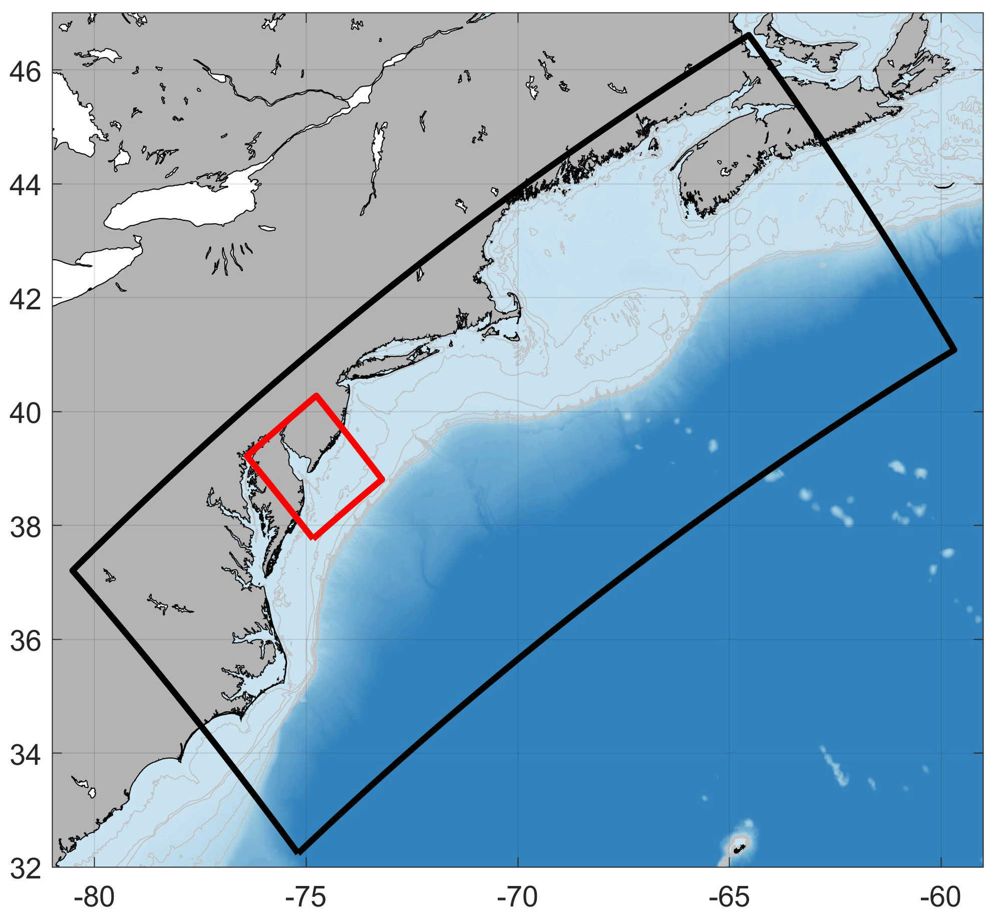
Figure 1 Map of the test domains. Black outlines the Doppio grid with ∼ 7 km resolution. Red outlines the SnailDel domain with ∼ 1 km resolution.

LTRANS can use a nested model output for particle tracking in principle but presently lacks the infrastructure to simultaneously process ROMS outputs from multiple grids in a nested grid hierarchy and seamlessly follow particles as they traverse the boundaries between parent and refinement grids. ROMSPath includes this functionality and draws hydrodynamic information from the most appropriate grid in the simulation. A representation of the grid decision tree is shown in Fig. 2. If the particle is inside a refinement grid, then ROMSPath uses velocities from that grid. Otherwise, it uses velocities from the parent grid. The grid that a particle is associated with is checked at every time step, starting with the highest resolution (smallest footprint) refinement grid. If the particle crosses a grid boundary its current grid is updated, its location is calculated in the new grid coordinate system, and advection continues on the new grid. Although the example shown here only uses one refinement grid, ROMSPath is capable of handling any number of refinement grids.

Open boundaries and coasts are handled in ROMSPath as they are in LTRANS. When a particle contacts an open boundary of the outermost domain, it is considered to have left the domain and its position is no longer tracked. When a particle encounters a closed boundary (surface, bottom, or coastline), it is reflected back into the domain by a distance equal to the distance it would have traveled past that closed boundary.

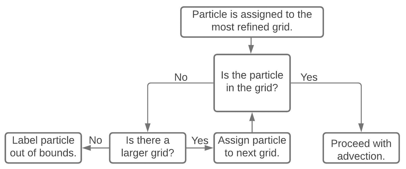
Figure 2 Flow diagram of the grid assignment process. At each time step particles are assigned to the most refined grid first. If the particle is determined to be within that grid domain, advection continues. If the particle is outside the domain, the next refined grid is checked. If the particle is not found to be within the domain of any grid, advection for that particle stops.

2.3 Vertical turbulent transport parameterization with split time stepping

The vertical component of velocity in the advection term (ΔX_hydro in Eq. 1) implicitly averages the timescales of displacements associated with subgrid-scale vertical turbulence that is unresolved by the hydrodynamic model. These motions are typically introduced in OPT models through the use of a “random walk” model applied to an ensemble of particles to represent the net dispersion that results. A vertical diffusion coefficient is required for such models to define the diffusive scales, and therefore ROMSPath requires that vertical tracer diffusivity be included in the ROMS output.

ROMSPath uses the same conceptual approach as LTRANS for implementing the vertical random walk, but it includes some changes. The vertical random walk algorithm is that of Hunter et al. (1993) and Visser (1997), which is designed for systems with spatially varying diffusivities. Specifically, for a simple random walk model, numerical imprecision inevitably leads to a clustering of particles in regions of low diffusivity (see Sect. 4.2). The modified vertical random walk, developed from consideration of the moments of the particle distribution, prevents such unrealistic particle clustering (Visser, 1997). The random walk is implemented in ROMSPath as

$$\begin{array}{}\text{(2)}& \mathrm{\Delta }{z}_{\mathrm{turb}}={\displaystyle \frac{\mathit{\delta }K}{\mathit{\delta }z}}\mathrm{\Delta }t+R{\left\{{\displaystyle \frac{\mathrm{2}}{r}}K\left[z_t+{\displaystyle \frac{\mathit{\delta }K}{\mathrm{2}\mathit{\delta }z}}\mathrm{\Delta }t\right]\right\}}^{\mathrm{1}/\mathrm{2}},\end{array}$$

where z is the particle's vertical location and K is the diffusivity reported by ROMS. R represents a random process with zero mean and a standard deviation equal to r. The vertical gradient of the diffusivity is extracted from the cubic spline interpolation of the diffusivity profile. This approach is common in other OPT models (Lett et al., 2008; Xue et al., 2008; van Sebille et al., 2018).

The algorithm described above reduces the clustering problem but requires a relatively short time step which can be computationally costly. In ROMSPath, we decouple the time steps for the random walk and advection, enabling the vertical diffusion model to run with a smaller time step than the advection model, thus reducing the computational cost without sacrificing a realistic distribution of particles due to vertical random processes. During the process of updating LTRANS to ROMSPath, we also noted an error in the implementation of the vertical random walk model, which resulted in an increase in unrealistic clustering when running LTRANS (see Sect. 3.3.2). Specifically, a sign error in the last term of Eq. (2) as it is implemented in the latest version of LTRANS led to increased particle clustering (see Sect. 4.2). This error is corrected in ROMSPath.

2.4 Wetting and drying

ROMSPath adds the capability to correctly handle particle transport when the ROMS option for wetting and drying (Warner et al., 2013) is activated. This option is useful in shallow, tidal, estuarine environments where mudflats can be above or below the waterline, depending on the phase of the tide. Wetting and drying in ROMS is implemented using a time-varying land mask to identify areas that transition from “wet” to “dry” when the depth of water above the seabed falls below a user-defined critical value. If ROMS has been run with wetting and drying (and the appropriate user flags are set), the time-varying mask is saved in the output. ROMSPath uses this mask to establish boundaries to advection that prevent a particle from entering a “dry” cell, which would lead to an ungraceful failure during execution. A particle encountering a “dry” cell will behave as if the cell is a land point, reflecting back into the “wet” cell. Particles occupying a cell that becomes dry will not move until the cell becomes wet again. Reading the wet–dry mask from the ROMS output at every time step increases the input/output (I/O) load slightly, but the increase in run time is minimal.

2.5 Stokes drift

Stokes drift can contribute to particle transport, particularly in nearshore, shallow-water environments (Feng et al., 2011; Monismith and Fong, 2004; Röhrs et al., 2012; Fuchs et al., 2018). However, few OPT models include a Stokes drift term in the advection scheme, presumably because the necessary wave information is not readily available. Some models, such as OpenDrift, allow for parameterizing Stokes drift based on the wind velocity. ROMS includes options to use wave information provided as external forcing data in the calculation of wave–current interaction effects on bottom drag and turbulent kinetic energy input at the sea surface due to wave breaking. In such configurations, the wave information is exported to the output and could be available to ROMSPath. In the event that these options are not active, including Stokes drift in ROMSPath requires an additional input that contains Stokes drift velocities stored on the ROMS grid and at ROMS output times. These velocities are calculated separately using output from a wave model, and read at the same time as the ROMS model output to calculate a Lagrangian velocity field as

$$\begin{array}{}\text{(3)}& {\mathit{V}}_{\mathrm{mean}}\left(\mathit{x},t\right)={\mathit{V}}_{\mathrm{hydro}}\left(\mathit{x},t\right)+{\mathit{V}}_{\mathrm{stokes}}\left(\mathit{x},t\right),\end{array}$$

where V_mean is the 4-D velocity field used by ROMSPath to determine ΔX_hydro in Eq. (1) for advection, V_hydro are velocities from the ROMS hydrodynamic files, and V_stokes are velocities from the Stokes drift files.

2.6 Behavioral inputs

LTRANS allows particle behaviors to vary as functions of the ROMS hydrodynamic variables (temperature or salinity). ROMSPath was developed for studies in which larval swimming behavior can also depend on flow vorticity and acceleration. These added behavioral inputs are incorporated in much the same way as Stokes drift, by reading files prepared offline with parameters stored on the ROMS grid, in both space and time. These parameters are interpolated to instantaneous particle positions and then used in ROMSPath to compute behavioral velocity, just as LTRANS does for temperature and salinity. This framework can be modified easily to allow other inputs for behavioral cues (e.g., irradiance). ROMSPath retains the LTRANS option for a simple vertical swimming behavior, where a constant vertical swimming velocity is specified and added to the particle's velocity vector V.

3 Test cases

3.1 ROMS model setup

We formulated test cases using 4-D hydrodynamic output from an existing implementation of ROMS in the northeast United States known as “Doppio” (López et al., 2020; Levin et al., 2019; Wilkin et al., 2018). The domain (shown in black in Fig. 1) has a horizontal resolution of ∼ 7 km and extends from the south of Cape Hatteras to Nova Scotia.

Forcing and boundary conditions are described by López et al. (2020). In short, meteorological forcing is provided by the North American Regional Reanalysis (NARR) (Mesinger et al., 2006) and the North American Mesoscale (NAM) forecast model (Janjic, 2005). River runoff is obtained from the United States Geological Survey (USGS) (http://waterdata.usgs.gov, last access: 24 May 2022) and the Water Survey of Canada (WSC) (https://wateroffice.ec.gc.ca/, last access: 24 May 2022​​​​​​​) and introduced as point sources of freshwater along the coastline. Open boundary conditions are daily mean data from the Mercator Océan system (Drévillon et al., 2014; Lellouche et al., 2018) with tidal constituents of sea level and velocity added from the Oregon State University Tidal Predication Software (Egbert and Erofeeva, 2002). Vertical mixing is parameterized using the generic length scale parameterization of Umlauf and Burchard (2003), configured to the closure described by Mellor and Yamada (1982). Horizontal mixing is parameterized as harmonic horizontal mixing along sigma surfaces for momentum, and geopotential surfaces for tracers.

The Doppio model setup in this study differs from López et al. (2020) in two ways. First, we took advantage of a previously developed data-assimilative Doppio implementation (Levin et al., 2019; Wilkin and Levin, 2021) by nudging temperature and salinity to the data-assimilative result with a 3 d timescale in waters with a bottom depth greater than 10 m. This nudging constrains the density field and mesoscale geostrophic velocity to remain close to the data-assimilative analysis without the added cost of re-running the data assimilation itself.

Second, the study that motivated ROMSPath investigated particle exchange between Delaware Bay and the adjacent shelf, so inside the Doppio domain we nested a fine-resolution grid named “SnailDel”. SnailDel (shown in red in Fig. 1) is a seven-fold refinement of the Doppio grid and has a horizontal resolution of ∼ 1 km. We implemented a coupled (two-way) nesting paradigm where the “parent” grid (Doppio) provides open boundary conditions to the “refinement” grid (SnailDel). Information feeds back to the Doppio domain by replacing the state variables at Doppio grid points within the SnailDel domain with spatially averaged SnailDel state variables. The seven-fold refinement used in this study reflects previous work investigating nested model configurations (Spall and Holland, 1991) and recent applications using the Doppio model (Warner et al., 2017). Meteorological forcing is the same as Doppio. River forcing is also from the USGS, although more river sources are in the SnailDel domain than the equivalent domain in Doppio.

For the examples shown here, hydrodynamic output was saved every 12 min of simulation for both model grids to meet specific scientific goals, such as resolving tidal variation in estuarine turbulence.

3.2 Wave model

Wave conditions were simulated for three uses: (1) to estimate whitecapping energy inputs to the ROMS turbulence model, (2) to determine Stokes drift for particle transport, and (3) to determine accelerations felt by particles for behavioral responses. We modeled waves using Simulating WAves Nearshore (SWAN), a third-generation spectral wave model (Booij et al., 1999; Ris et al., 1999). SWAN was run independently from the Doppio/SnailDel nested hydrodynamic run, and ROMS and SWAN were not directly coupled. The SWAN model grids for SnailDel and Doppio are colocated with the ROMS grids and use the same bathymetry. The SWAN grids were nested one-way, with the SnailDel grid receiving wave open boundary conditions from the SWAN–Doppio grid, while Doppio used wave open boundary conditions from NOAA Wavewatch III (Tolman, 2009). Meteorological forcings for the SWAN model runs are the same as for the ROMS hydrodynamic runs, and output is saved at the same frequency.

The turbulence surface boundary condition for ROMS was determined using methods similar to those described in Gerbi et al. (2015) and Thomson et al. (2016). Stokes drift was calculated from the directional wave spectrum following Eq. (3.3.5) in Phillips (1966), and saved in separate files for use in ROMSPath.

3.3 Configurations

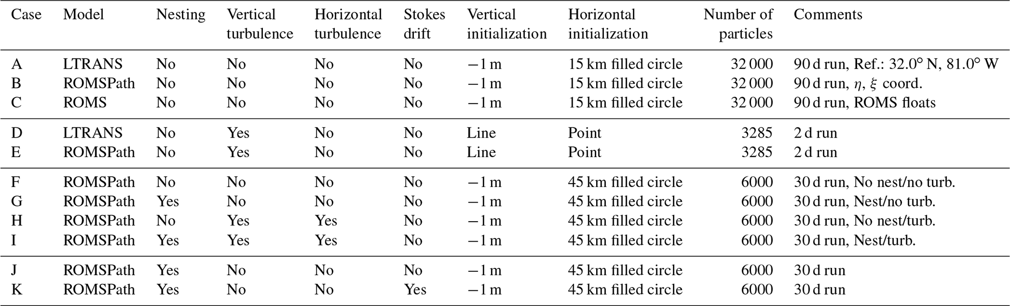
One motivation for the development of ROMSPath was to enable the use of a nested grid output from ROMS, which led to a number of useful changes to the underlying code (ROMS grid coordinates, turbulence, wetting and drying). We performed 11 simulations (designated A–K​​​​​​​) to evaluate many of these changes. The configurations for each of these tests are described here, and summarized in Table 1. Results are described in Sect. 4.

Table 1 Particle tracking model simulation configurations for cases A–K. All cases use either LTRANS, ROMSPath, or the ROMS online float subroutine as an advection model. Cases with nesting use data from both SnailDel and Doppio for advection while cases without nesting include Doppio data only. The vertical turbulence parameterization is used in cases D, E, H, and I only, and horizontal turbulence is used in cases H and I. Stokes drift was active in case K only. Particles in all cases except D and E are initialized at −1 m depth and randomly distributed in a circle. In cases D and E particles are evenly spaced vertically (∼ 34 m depth) at a single horizontal location.

3.3.1 Coordinate system

We evaluated the simulation of particle trajectories on the ROMS native coordinate system using ROMSPath in comparison to the intermediate coordinate system used in LTRANS. The results are compared, further, to the ROMS online particle tracking system referred to here as ROMS floats. ROMS float particle trajectories are integrated using a fourth-order Milne predictor and a fourth-order Hamming corrector, which are arguably less accurate than ROMSPath, but the calculation is made on every model time step; hence we believe the ROMS floats results represent the most accurate trajectories possible.

We compare three simulations: one via LTRANS which simulates trajectories on an intermediate coordinate system defined using the recommended reference position for the projection (Schlag and North, 2012) (case A); one via ROMSPath which operates on the ROMS native coordinate system (Supplement Fig. S1) (case B); and one using ROMS floats (case C). All three simulations used the same initial particle positions and omitted horizontal and vertical turbulence components. For each case, 32 000 particles were randomly distributed throughout a circle 20 km in diameter at 1 m below the sea surface and released. A Doppio simulation (without nesting) that also activated ROMS floats is run for 90 d and a hydrodynamic output is saved every 12 min. These hydrodynamic outputs are used as input to the LTRANS and ROMSPath simulations. A 90 d run time is chosen as it allows sufficient time for particles to exit the Mid-Atlantic Bight shelf and 32 000 particles are necessary to maintain coherent patches for comparison.

3.3.2 Turbulence parameterization

In order to illustrate the impact of an error in the LTRANS vertical turbulence parameterization, we configured two similar runs for LTRANS (case D) and ROMSPath (case F). Both runs are initialized at the same location with 3285 points evenly distributed in the vertical dimension (∼ 34 m depth), similar to Visser (1997). For this test, LTRANS was coded to include a short time step for turbulence and a longer time step for advection. Note that this capability is not native to LTRANS. The turbulent time step is set to 1 s and the advection time step was set to 60 s for both ROMSPath and LTRANS. Both simulations are run for 2 d, long enough to observe significant differences in turbulent mixing.

Figure 3 Comparison of particle positions from LTRANS (case A, green), ROMSPath (case B, blue) and ROMS floats (case C, yellow). ROMS floats represents the most accurate available estimates. For clarity, we show separate comparison of LTRANS versus ROMS floats (a, c, e) and ROMSPath versus ROMS floats (b, d, f). Dots are particle positions at day 5 (a–b), 35 (c–d), and 90 (e–f), and solid lines in (a) and (b) are the centers of mass of particle trajectories over the 90 d simulation. The ROMSPath simulations are more consistent with ROMS floats simulations in dispersion, offshore transport, and trajectory of the center of mass.

3.3.3 Nesting and vertical/horizontal turbulence

Most numerical models include schemes for vertical and horizontal mixing by unresolved (turbulent) processes, and the magnitude of the mixing coefficients generally vary with the resolution of the grid. Finer grids allow more direct simulation, rather than parameterized simulation, of dynamics and particle trajectories. Because finer grids resolve more processes, the mixing coefficients represent fewer unresolved processes and are therefore smaller. We examined the effect of grid resolution (via the inclusion of nesting) and vertical/horizontal turbulence on particle trajectories using a set of four simulations with the same initial conditions (Table 1, cases F–I). The velocity fields used for particle tracking all came from the same hydrodynamic simulations but were used in different ways. All of the hydrodynamic simulations included horizontal mixing (see Sect. 3.1), but in the particle tracking models, horizontal mixing coefficients were not always used. Case F does not use nested output in the OPT model and thus only uses velocities from the Doppio grid (∼ 7 km resolution). Furthermore, no horizontal or vertical turbulent parameterizations are supplied during this OPT run. Case G uses a nested hydrodynamic output; i.e., velocities were from both Doppio (∼ 7 km resolution) and SnailDel (∼ 1 km resolution) outputs, but did not include horizontal or vertical turbulent parameterizations. The third (case H) and fourth (case I) cases are similar to the first two, except that horizontal and vertical mixing were turned on.

In each simulation, 6000 neutrally buoyant particles are initially distributed randomly in a circle (45 km diameter) at 1 m below the sea surface. The initial condition is located off the central New Jersey coast, just north of the SnailDel domain. Particles were tracked for 30 d after release, and 100 % of the released particles entered the boundaries of the SnailDel domain at some point during the simulation. A run time of 30 d with 6000 particles provided enough time for particles to leave the SnailDel domain while maintaining a coherent patch of particles.

3.3.4 Stokes drift

We compare two OPT runs (case J and case K, Table 1) to test how adding Stokes velocities to the hydrodynamic velocities impacted particle trajectories. Case J is identical to case G from Sect. 3.3.3, while case K adds Stokes drift from surface gravity waves according to Eq. (3).

4 Results and discussion

Here we examine the results of the exploratory simulations described in Sect. 3.3. This examination does not cover all the differences between LTRANS and ROMSPath, but instead focuses on demonstrating the utility of the most important changes.

4.1 Coordinate system

The ROMSPath output is always closest to the ROMS floats output when we compare cases A–C. Particle trajectories from three simulations, using LTRANS (case A), ROMSPath (case B), and ROMS floats (case C), are compared in Fig. 3. Although all results are similar after 5 d, the discrepancy in LTRANS outputs grows large by 35 d. Compared to LTRANS, the ROMSPath data more accurately reflect the variability of the particles' center of mass seen in the ROMS floats data (Fig. 3a). Although the center of mass of LTRANS and ROMS floats data appear to nearly intersect in space, they reach that point at different times. The center of mass becomes a less useful metric over time as the distributions become non-Gaussian when particles begin to leave the shelf. In particular, the LTRANS fails to reproduce the off-shelf transport and entrainment of particles into the Gulf Stream seen in the ROMS floats output. This off-shelf transport leads to a large dispersal of particles between the Gulf Stream and the Mid-Atlantic Bight shelf break, which is well represented in the ROMSPath output.

Following Simons et al. (2013), we calculate particle density distributions for cases A–C at every time step. A spatial correlation between cases is then calculated at each model time and shown in Fig. 4. The case B to case A correlation remains at or above 0.9​​​​​​​ for the first 25 d of the run time and remains above 0.7 for the rest of the simulation. By comparison, the case A to case C correlations drop below 0.7​​​​​​​ in the first 10 d, and drop to <0.5 afterwards. It is interesting to note that there are few examples of direct comparisons between an online and offline Lagrangian model output such as this. In most cases it is a comparison of the online solution for a tracer advection–diffusion equation to offline particle tracking, both in the atmosphere (Cassiani et al., 2016) and the ocean (Wagner et al., 2019). In the ocean (Wagner et al., 2019) it is used to validate offline particle tracking as a proxy for tracer advection, with success in simulating tracer horizontal dispersion and mean tracer pathways. This suggests that simulating tracer fields at a regional scale is a potential use for ROMSPath, although more investigation is required.

In this comparison, we also found that ROMSPath (case B) was more successful than LTRANS (case A) at keeping particles from running aground. ROMSPath enforces a kinematic boundary condition of no flow across the discrete coastline, which is absent in LTRANS. In LTRANS, approximately 34 % of particles pass through a “land” grid cell during the simulation. Less than 0.01 % of particles pass through land cells in ROMSPath. This added boundary condition reduces the number of particles lost to unrealistic running aground.

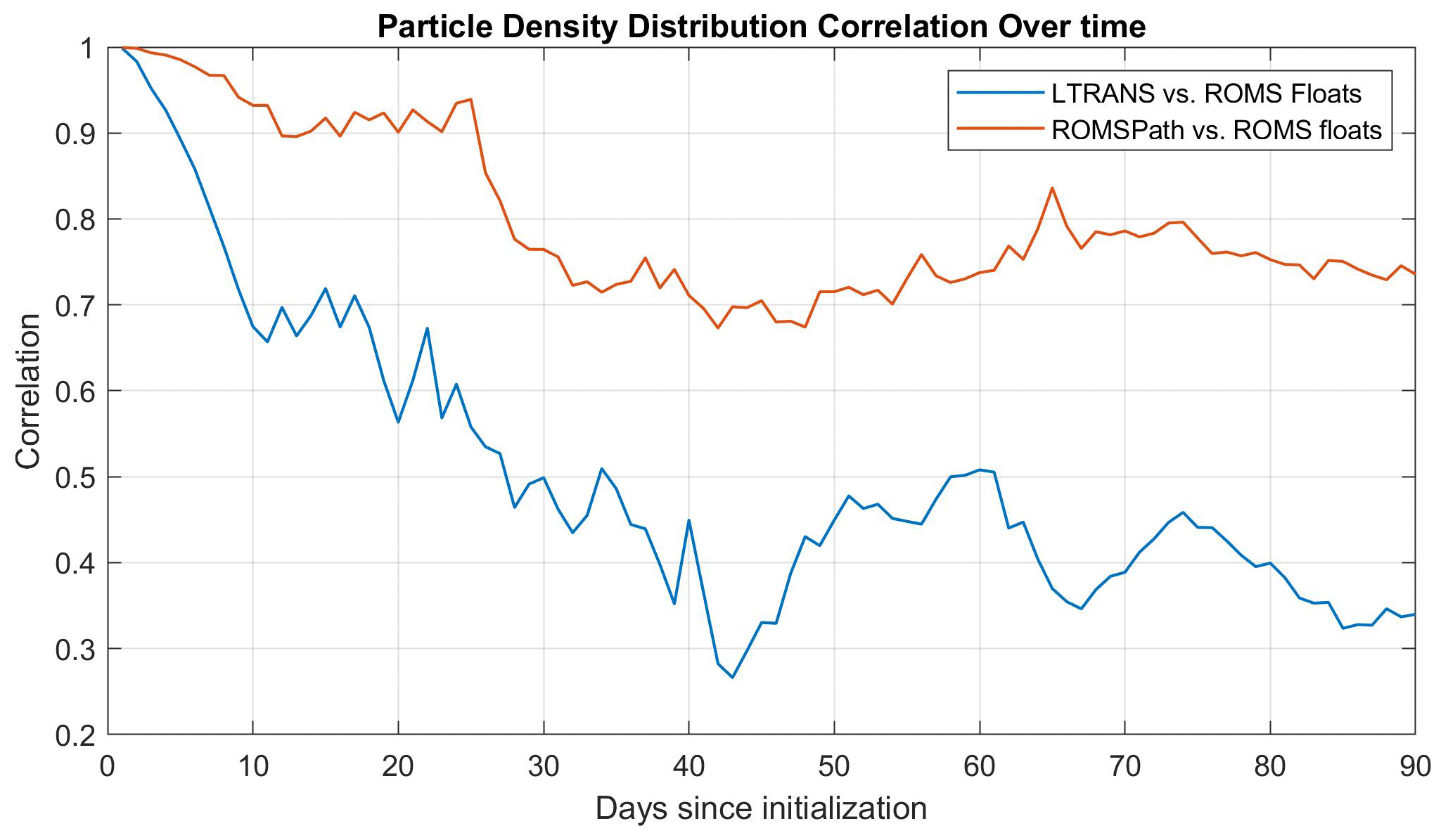
Figure 4 Comparison of particle density distributions over time (Simons et al., 2013). Spatial correlations between ROMSPath (case B) and ROMS floats (case C) are greater than 0.7​​​​​​​ for most of the run time. The LTRANS (case A) correlations (with case C) drop below 0.7 within 10 d.

4.2 Vertical interpolation, split time stepping, and turbulence

The LTRANS vertical turbulence parameterization leads to clustering in areas of low diffusivity. Figure 5 shows a comparison of the vertical distribution for LTRANS (case D) versus ROMSPath (case E) (Table 1). Figure 5a and b both show particle density distributions in the vertical dimension over the 2 d period of the simulations. A representative tracer diffusivity profile is overlaid for context. The LTRANS data show a particle density maximum at the tracer diffusivity minimum. We note from previous work (Supplement Fig. S2) that the clustering problem would be mitigated by using a small enough advective time step in LTRANS, similar to the scale of the turbulent time step. However, the small time step required has severe consequences for computation speed, particularly for OPT runs with tens of thousands of particles.

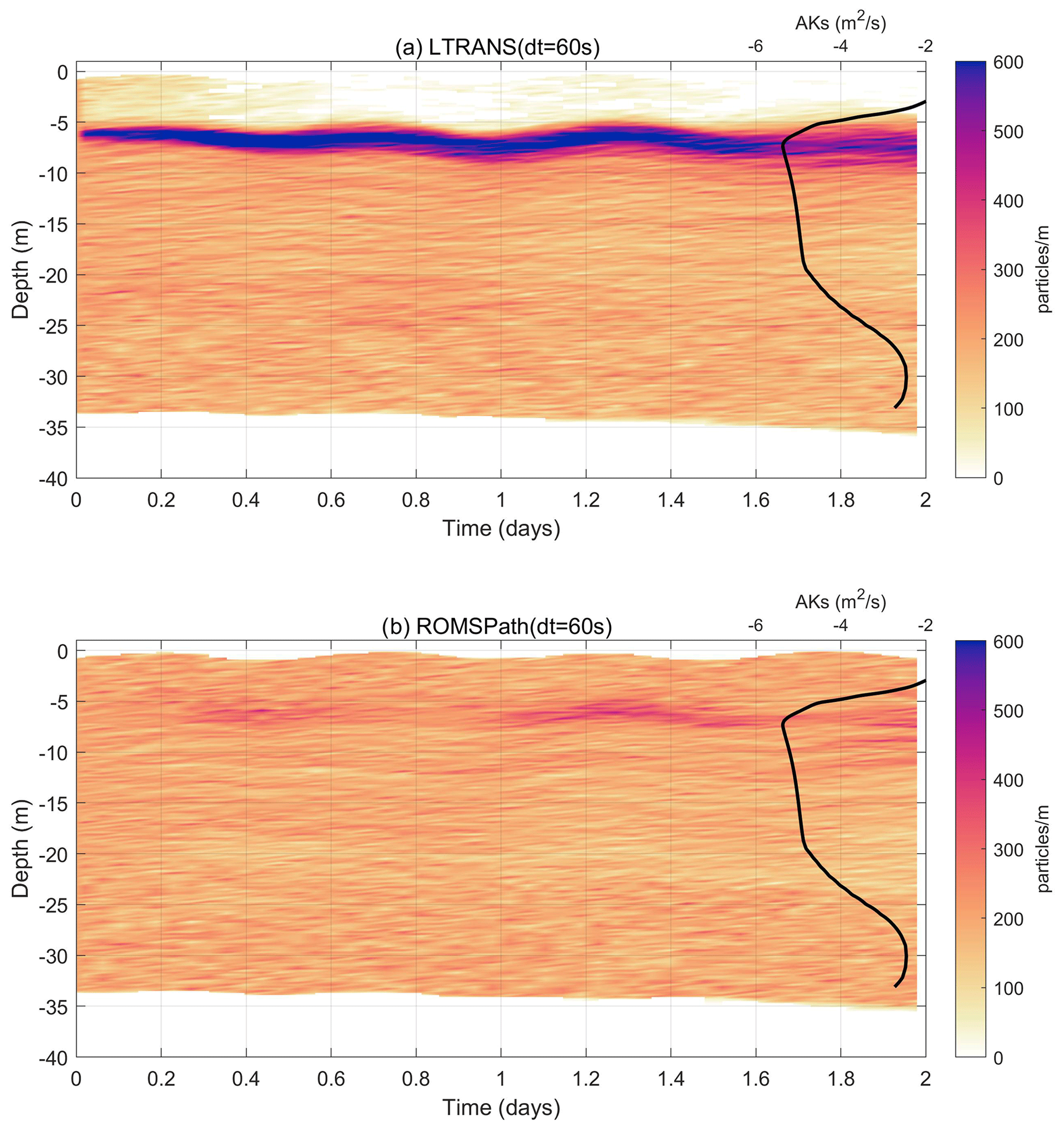
Figure 5 Vertical density of particles over time for the (a) LTRANS run (case D) and the ROMSPath run (case E). Both runs used a 60 s time step and were initialized at the same horizontal location and time, with 3285 particles evenly. A representative vertical tracer diffusivity (log10(AKs)) is overlaid in black. The LTRANS run has particle clustering at the vertical diffusivity minimum due to a sign error in the vertical turbulence module.

4.3 Nesting and horizontal mixing

The nesting and mixing comparisons (Fig. 6) showed that particle dispersion is enhanced by the use of nested grid outputs even when there is no horizontal mixing. We first compare the unnested (case F) and nested (case G) runs with no turbulence. The addition of a nested grid increased the horizontal diffusivities of particles (LaCasce, 2008) from 345 to 452 m² s⁻¹ (Fig. 6a, c, e, g). With no nesting or turbulence (case F), particle trajectories showed coherent structures over time, with some horizontal deformation and little or no vertical dispersion (Fig. 6a, b). The addition of the nested SnailDel grid (case G) reveals the importance of small-scale hydrodynamic features. Outside of the SnailDel domain (Fig. 6c, d), the particle transport/dispersion was similar to the unnested case, but inside SnailDel, there was more horizontal dispersion when the nested grid was included (Fig. 6c), enabling some particles to enter Delaware Bay. The vertical distribution of particles in Fig. 6d suggests particles were more likely to disperse to deeper waters. The time-averaged, near-bottom currents at the mouth of Delaware Bay are directed into the estuary (Garvine, 1991), providing a pathway for particles on the shelf to enter the bay. There is no vertical or horizontal mixing parameterized in these two cases, suggesting that smaller-scale features, such as fronts, jets, or subduction, resolved by the SnailDel grid (and accessed via nested OPT) allow for enhanced dispersion in the horizontal and vertical dimension relative to the Doppio grid alone.

Particle dispersion is further enhanced with the addition of horizontal and vertical mixing (Fig. 6e–h). Here we compare the unnested (case H) and nested (case I) runs with turbulence. When horizontal and vertical mixing are parameterized, dispersion increased in all directions relative to the runs with no turbulence. However, in the two runs with turbulence, there are also greater vertical and horizontal dispersion in the nested run compared to the unnested run (Fig. 6e, f compared to Fig. 6g, h). With turbulence, the horizontal particle diffusivities were 525 and 570 m² s⁻¹ for the unnested and nested cases, respectively. Nesting and turbulence parameterizations improve resolution of small-scale hydrodynamics, and including both in ROMSPath simulations provides the most dispersion and, for this example, the largest transport of particles into Delaware Bay.

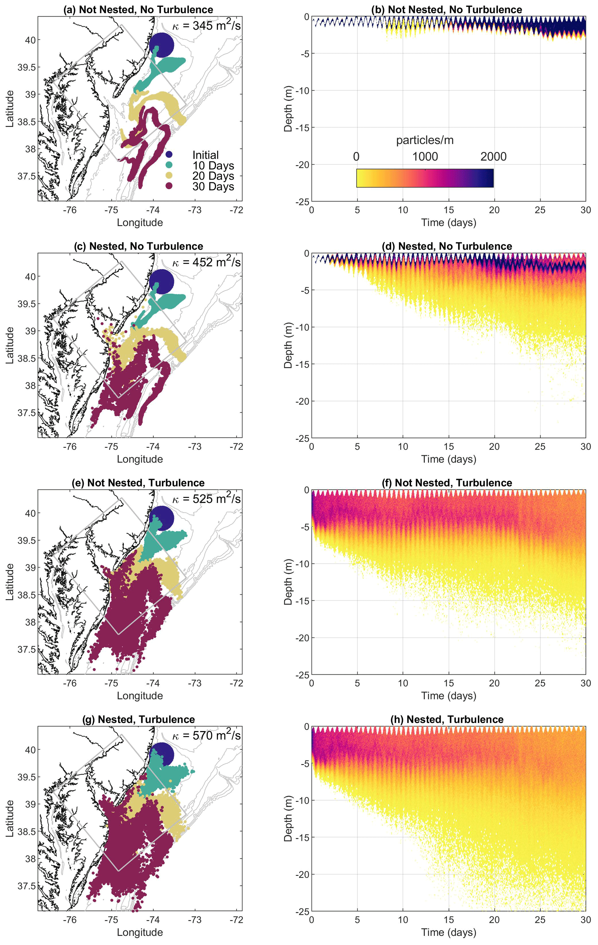
Figure 6 ROMSPath simulations showing particle locations (a, c, e, and g) after 10, 20, and 30 d and vertical particle distributions (b, d, f, and h) over time. Panels (a)–(h) show ROMSPath runs with and without a nested grid and turbulence. The grey box in (a), (c), (e), (g) is the boundary of the SnailDel domain. Diffusivity (κ) for each case is shown in the upper right of panels (a), (c), (e), and (g).

4.4 Stokes drift

The addition of Stokes drift modified trajectories and increased particles' movement onshore. Here we compare two runs without (case J) and with (case K) Stokes drift (Table 1, Fig. 7a and b, respectively). The wave field associated with the Stokes velocities was generally swell (6–10 s period) to the north/west (Fig. 7c). Given the orientation of the coastline (southwest to northeast), wave swell was onshore during this time period. Results from the two runs showed a tendency for particles to go farther into Delaware Bay and move closer to the coastline when Stokes drift was included. For example, the particles' ending center of mass was 9 km closer to shore with Stokes drift than without, and after 30 d, more particles were in water depths <50 m with Stokes drift (57 %) than without (38 %) (Fig. 8).

These runs used neutrally buoyant particles, and we would expect a greater impact of Stokes drift on the transport of particles with positive buoyancy or upward swimming. Stokes velocities are on the order of Eulerian velocities at times and are largest near the surface (Monismith and Fong, 2004). This additional transport has implications for tracer transport (Monismith and Fong, 2004; van den Bremer and Breivik, 2018), estuary–shelf exchange (Pareja-Roman et al., 2019; Fuchs et al., 2018), larval transport/recruitment (Feng et al., 2011), and nearshore processes (Kumar and Feddersen, 2017a, b). The option to include Stokes velocities expands opportunities for ROMSPath users to investigate these processes.

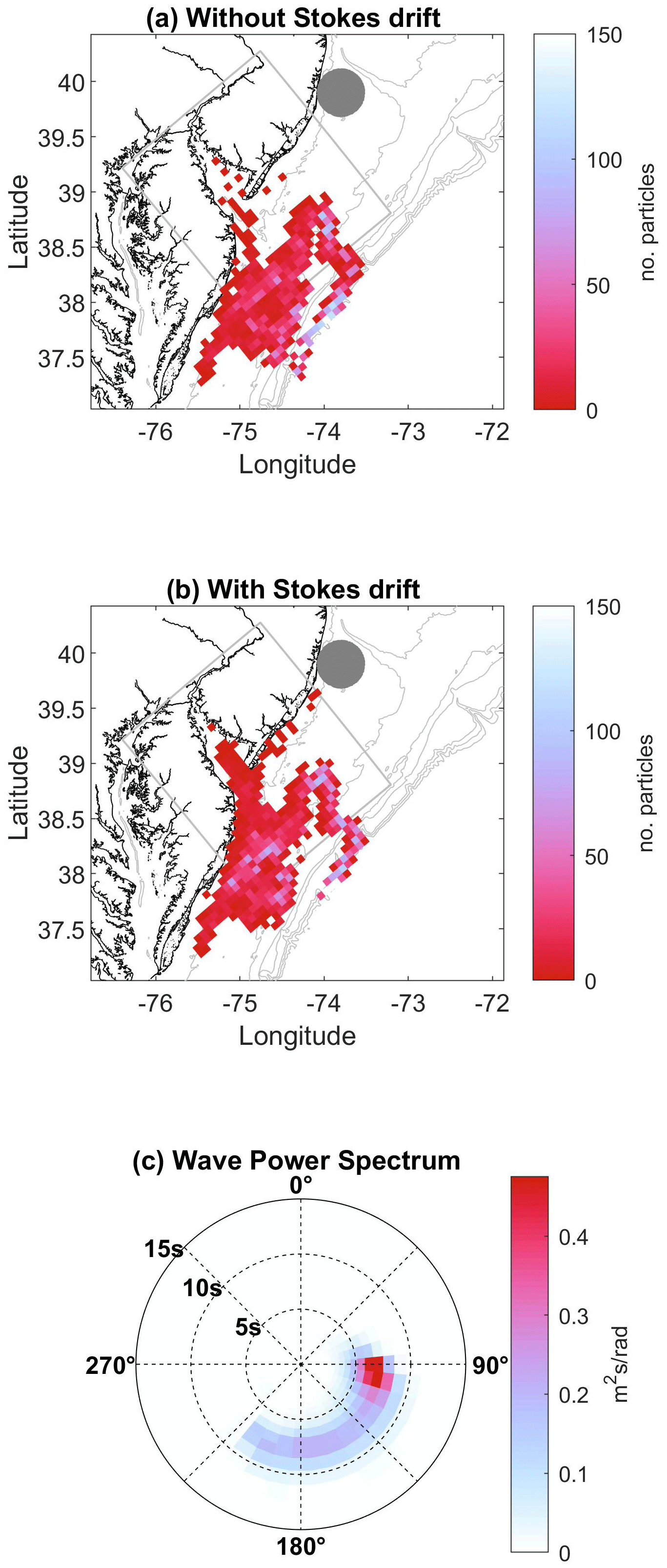
Figure 7 ROMSPath simulations showing particle distributions after 30 d (a) without Stokes drift (case J), and (b) with Stokes drift (case K). The mean directional wave spectrum (c) is shown from the SWAN model output in the SnailDel domain over the 30 d release period (direction is the direction waves come from). Particle initial locations are designated by the dark grey circle. In this example, more particles enter the bay when Stokes drift is included than when it is omitted, consistent with waves entering the domain from the southwest.

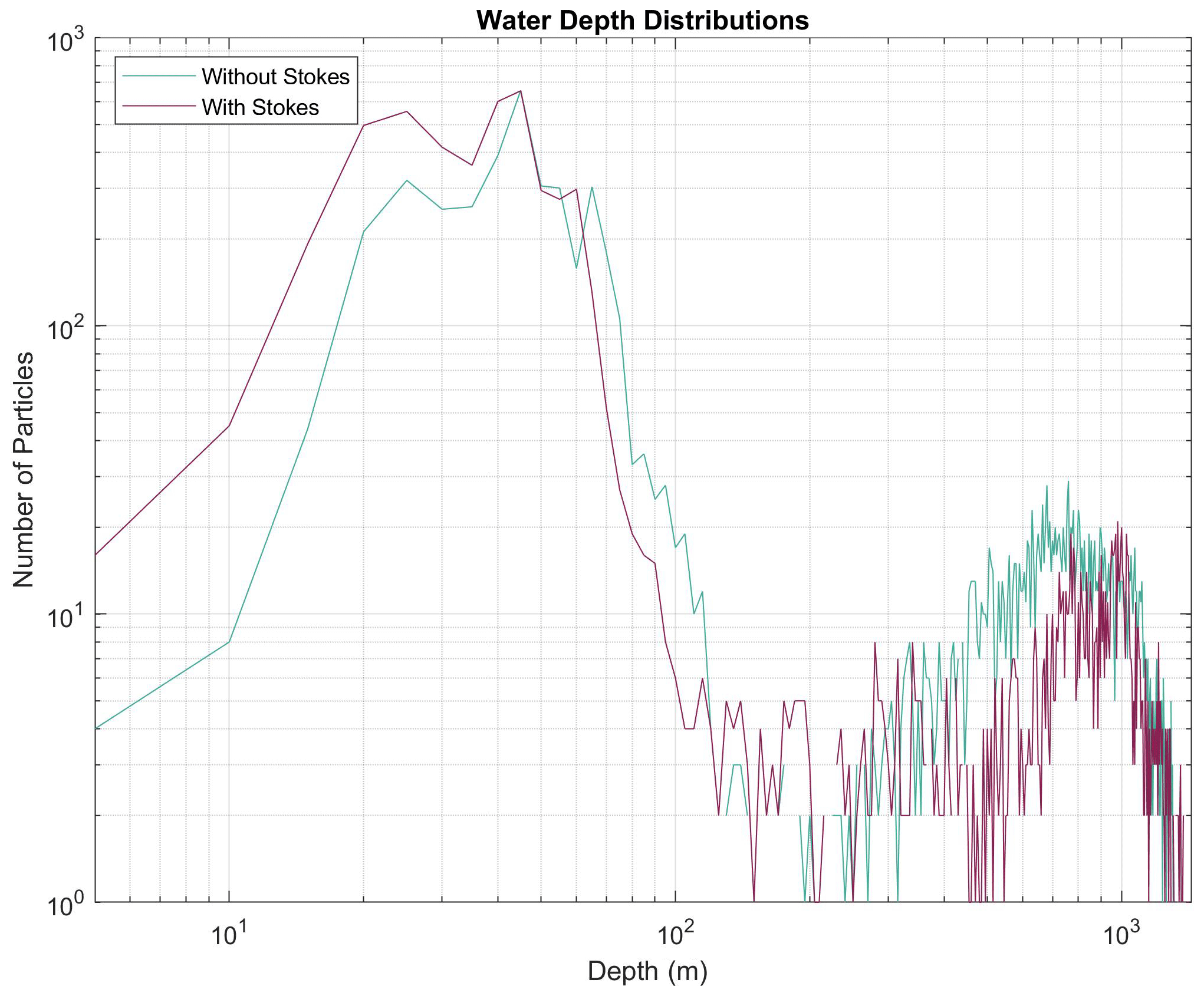
Figure 8 Total water depth at particle locations for cases without Stokes drift (J) and with Stokes drift (K). The histograms show depths after 30 d of simulation. More particles ended in water depths less than 50 m when Stokes drift was included (57 %) than when it was omitted (38 %).

5 New feature summary

OPT models are a useful tool for investigating a wide range of physical, chemical and biological processes in the world's oceans. As such, these models are continuously improved. Here we introduced updates to a widely used and successful OPT model (LTRANS), which we release under the name of ROMSPath. The base coordinate system used for advection in ROMSPath is now ROMS' ξ ,η coordinates, improving accuracy and efficiency. ROMSPath also has the flexibility to use output from multiple ROMS nested grids, enabling particle tracking across grid resolutions at execution time. A correction to the vertical mixing parameterization helps to reduce clustering in regions where diffusivity gradients are large, while the ability to split the advective and diffusive time steps increases numerical efficiency and speed to make the use of appropriate time steps more practical. Finally, functionality for the addition of Stokes and/or behavioral velocities to the hydrodynamic velocity output from ROMS is included. These features proved valuable in recent investigations of harmful algal blooms in the Gulf of Maine (Clark et al., 2021) and the retention of larvae in Delaware Bay (Garwood et al., 2022).

These changes improve the computational performance of ROMSPath compared to LTRANS. It is difficult to quantify separately the improvements in numerical efficiency and computing speed. Speed depends partly on specifics of the computational system, and detailed performance tests were outside the scope of this work. However, speed typically increased by 20 % to 30 % for the simulations shown here and up to 4000 % for simulations in our scientific study (Garwood et al., 2022). These ROMSPath improvements create opportunities to conduct more extensive numerical experiments with the finite computing resources that researchers have available.