the Creative Commons Attribution 4.0 License.
the Creative Commons Attribution 4.0 License.
 | 01 Jun 2022
Evaluating a reservoir parametrization in the vector-based global routing model mizuRoute (v2.0.1) for Earth system model coupling
Shervan Gharari
Naoki Mizukami
Martyn P. Clark
David M. Lawrence
Sean Swenson
Yadu Pokhrel
Naota Hanasaki
Ann van Griensven
Wim Thiery
Human-controlled reservoirs have a large influence on the global water cycle. While global hydrological models use generic parameterizations to model dam operations, the representation of reservoir regulation is still lacking in many Earth system models. Here we implement and evaluate a widely used reservoir parametrization in the global river-routing model mizuRoute, which operates on a vector-based river network resolving individual lakes and reservoirs and is currently being coupled to an Earth system model. We develop an approach to determine the downstream area over which to aggregate irrigation water demand per reservoir. The implementation of managed reservoirs is evaluated by comparing them to simulations ignoring inland waters and simulations with reservoirs represented as natural lakes using (i) local simulations for 26 individual reservoirs driven by observed inflows and (ii) global-domain simulations driven by runoff from the Community Land Model. The local simulations show the clear added value of the reservoir parametrization, especially for simulating storage for large reservoirs with a multi-year storage capacity. In the global-domain application, the implementation of reservoirs shows an improvement in outflow and storage compared to the no-reservoir simulation, but a similar performance is found compared to the natural lake parametrization. The limited impact of reservoirs on skill statistics could be attributed to biases in simulated river discharge, mainly originating from biases in simulated runoff from the Community Land Model. Finally, the comparison of modelled monthly streamflow indices against observations highlights that including dam operations improves the streamflow simulation compared to ignoring lakes and reservoirs. This study overall underlines the need to further develop and test runoff simulations and water management parameterizations in order to improve the representation of anthropogenic interference of the terrestrial water cycle in Earth system models.
- Article
(6365 KB) - Full-text XML
- BibTeX
- EndNote


The terrestrial global water cycle is fundamentally altered by human activities like groundwater pumping, river water abstraction for irrigation, and the construction of large dams (Oki and Kanae, 2006; Rockström et al., 2009; Wada et al., 2014). Worldwide, more than 45 000 large dams have been built to create reservoirs that provide hydropower, irrigation, or drinking water supply or are used for flood control (Lehner et al., 2011; Sterl et al., 2020). Reservoir expansion since the 20th century impounded at least 8300 km3 of water (Chao et al., 2008), counteracting global sea level rise by around 30 mm (Chao et al., 2008; Frederikse et al., 2020) and redistributing heat contained within the world's water resources, increasing anthropogenic heat uptake by inland waters (Vanderkelen et al., 2020). By buffering seasonal river flow, reservoirs control more than half of the variability in global surface water storage (Cooley et al., 2021) and can substantially alter the timing and volume of natural streamflow (Döll et al., 2009). Today, more than 77 % of global rivers are human regulated or are interrupted by dams, reservoirs, or other infrastructure (Grill et al., 2019). Therefore, accounting for reservoirs and dam operations is important when assessing the seasonality of global streamflow and water availability (Nazemi and Wheater, 2015a; Pokhrel et al., 2016).
Despite the clear human imprint on the terrestrial water cycle, Earth system models generally do not yet account for human alterations to flow by dam operations in their component land models (Pokhrel et al., 2016). However, to adequately understand human alterations to flow it is key to represent dam management in holistic modelling frameworks covering all Earth system components (Nazemi and Wheater, 2015b; Pokhrel et al., 2016). Recent efforts are beginning to address this limitation. For example, Zhou et al. (2020) coupled the MOSART-WM, a river-routing and water management model including reservoir operation, to the land model of E3SM. Also in MIROC-INTEG-LAND, water management modules have recently been incorporated in the land component of the MIROC Earth system model, together with crop production, land ecosystem, and land use modules (Yokohata et al., 2020). Overall, these developments suggest that reservoir management could potentially be considered in upcoming rounds of the Coupled Model Intercomparison Project (CMIP; Eyring et al., 2016) or other multi-model assessments.
Due to their importance for water resource assessments, reservoir operations have long since been represented in large-scale hydrological models, including catchment models (e.g. Chawanda et al., 2020; Shin et al., 2019), water management models (e.g. Voisin et al., 2013b, a), and global hydrological models (GHMs; see Sood and Smakhtin, 2015, and Telteu et al., 2021, for a comprehensive overview). However, substantial variations in operating rules and the lack of operational knowledge of reservoirs worldwide necessitate the use of generic parameterizations to describe reservoir operations (Pokhrel et al., 2016). Such generic schemes are typically not designed to reproduce the daily operations of individual reservoirs, but they provide simple, yet widely applicable rules, mimicking human decisions in regulating dams to the greatest extent possible. A wide range of approaches exist, which can broadly be categorized into optimization-based methods (e.g. Haddeland et al., 2006), methods based on target storage and release (e.g. Burek et al., 2013; Yassin et al., 2019), and inflow-and-demand-based methods (e.g. Wisser et al., 2010; Hanasaki et al., 2006). In addition to these approaches, which do not require prior information on historical reservoir operations, there are also a wide variety of reservoir models that use operational data for specific reservoirs to develop general operational rules (e.g. Coerver et al., 2018; Zhao et al., 2016; Ehsani et al., 2016) and extrapolate these empirical operating rules to data-scarce reservoirs with similar operating purposes and hydrologic conditions (Turner et al., 2021). For a comprehensive overview of the range of existing reservoir parameterizations, their characteristics, advantages, and disadvantages, the reader is referred to Pokhrel et al. (2016); Yassin et al. (2019) and Gutenson et al. (2020).
Here, we evaluate the representation of reservoirs in the state-of-the art river-routing model mizuRoute (Mizukami et al., 2016, 2021), in view of its anticipated coupling in the Community Land Model (CLM), the land component of the Community Earth System Model (CESM). The CLM modelling framework already accounts for historical reservoir construction by including lake area expansion (Vanderkelen et al., 2021), but an explicit representation of lake and reservoir water balance dynamics is currently lacking. We investigate the effect of dam operations on river flow when using the parametrization of Hanasaki et al. (2006) in mizuRoute. Compared to other reservoir models, the Hanasaki parametrization has low data requirements (it only needs information on irrigation water demand and instantaneous inflow) and does not require prior knowledge (e.g. of future inflows, like the schemes derived from the Haddeland et al., 2006, parametrization) and can thus be used instantaneously during a simulation. Moreover, due to its generic nature, the Hanasaki parameterization can be applied to every reservoir across the globe. Therefore, the Hanasaki parametrization has been widely used as a basis in large-scale hydrological modelling studies (e.g. Biemans et al., 2011; Voisin et al., 2013a; Droppers et al., 2020; Döll et al., 2009; Hanasaki et al., 2008; Pokhrel et al., 2012; Shin et al., 2019).
In contrast to previous studies, we evaluate the implementation of the Hanasaki et al. (2006) parametrization in a global river-routing model that operates on a vector-based river network, mizuRoute. To provide seasonal irrigation demand per reservoir, we develop an irrigation topology, which defines the area over which the water demand is aggregated for an individual reservoir based on the river network topology and catchments. We evaluate the added value of the Hanasaki et al. (2006) parametrization for reservoir outflow and storage modelling in a stand-alone mizuRoute simulation that uses reservoir observations as input and compare results to a simulation using the natural lake outflow parametrization of Döll et al. (2003). Next, both parameterizations are evaluated using mizuRoute in a global routing-only application with runoff input from CLM to evaluate their capability to represent outflow and storage at individual reservoirs and to capture long-term trends in monthly streamflow indices. Our modelling framework enables us to identify biases in runoff from CLM by comparing variables that have not previously been modelled (e.g. reservoir outflow and storage) to observations. Finally, we explore new avenues for future model development and towards coupling within CESM. This study provides an essential step towards incorporating human water management and reservoir dynamics in a coupled Earth system model, which enables investigating complex interactions between climate change, human water management, and natural systems in an integrated holistic framework. In addition, including reservoir operations in CLM will allow us to investigate the potential of water management strategies to mitigate climate change impacts on water resources.
2.1 mizuRoute
The vector-based routing model mizuRoute is designed to use runoff provided by hydrological models or land models and simulate spatially distributed streamflow (Mizukami et al., 2016, 2021). The routing is performed in two steps: first, basin runoff is routed from the hillslopes to the river reach with a gamma-distribution-based unit hydrograph. Following this, the water is routed downstream through the river channel network using either an impulse response function (IRF) or a kinematic wave tracking (KWT) routing scheme (Mizukami et al., 2016). In stand-alone applications, mizuRoute internally remaps the gridded runoff provided by the land model or hydrological model to the basin defined in the vector-based river network. In continental or global applications, mizuRoute provides a spatial decomposition of the river networks to allow for parallel routing computations (Mizukami et al., 2021). Natural lakes and reservoirs are integrated in the vector-based river network as hydrological features with additional parameters including information on the characteristics of the lake and/or reservoir, like maximum capacity (Gharari et al., 2022). This approach allows the lake and reservoir water balance to be modelled using data on precipitation and evaporation from the water surface in combination with parameterizations providing information on the releases, including both natural outflow and regulated discharge. For this study, the IRF routing scheme was used for river channel routing that produces the discharge into lakes and reservoirs.
2.2 Lake and reservoir parameterizations
Gharari et al. (2022) introduces parametric lake and reservoir implementations in mizuRoute to simulate lake and reservoir outflow. Natural lakes are modelled as linear reservoirs using the parametrization of Döll et al. (2003) (Eq. 1), which resolves daily outflow (Qdaily in m3 s−1) as a function of current active lake storage (S in m3) with a release coefficient kr (taken constant at 0.01 s−1) and the maximal lake storage capacity (Smax in m3). The exponent in the parametrization is determined based on the theoretical value of outflow over a rectangular weir (Meigh et al., 1999).
In this study, we investigate the impact of implementing management of human-constructed reservoirs and dam-controlled lakes with the parametrization described in Hanasaki et al. (2006). This algorithm minimizes intra- and inter-annual variability, while accounting for irrigation and other water demands, making a distinction between reservoirs used for irrigation and other purposes such as hydropower, flood control, navigation, or water supply. Irrigation reservoirs, which provide water for crops downstream, are characterized by a distinct seasonal variability guided by the downstream irrigation water needs. Since withdrawal periods do not necessarily coincide with high inflow periods, the parametrization explicitly accounts for the downstream irrigation demand in the intra-annual outflow. The reservoirs with purposes other than irrigation are operated in the same way, aiming to reduce intra- and inter-annual flow variability. Furthermore, the parametrization differentiates between “multi-year reservoirs” with high storage capacity compared to their annual inflow and “within-a-year reservoirs”, defined as reservoirs with annual inflow values that are more than half of the storage capacity. Within-a-year reservoirs carry the inflow seasonality in their outflow values to compensate for potential overflow and storage depletion, while multi-year reservoirs aim to maintain a constant outflow (Hanasaki et al., 2006).
Below, we outline the parametrization as described in Hanasaki et al. (2006) and specify how it is implemented in mizuRoute. The parametrization uses operational years, which are unique to every reservoir and different from the calendar year. The operational year starts on the first day of the month in which the multi-year monthly inflow drops below the annual inflow (Hanasaki et al., 2006; Haddeland et al., 2006). Following this, at the start of the operational year the monthly target release is determined based on the purpose of the reservoir. For non-irrigation reservoirs the monthly target release Qtarget (m3 s−1) is taken as the annual mean inflow Imean (m3 s−1; Eq. 2).
For irrigation reservoirs, the target release is calculated by Eq. (3),
with Im (m3 s−1) the mean monthly inflow for the corresponding month, Imean (m3 s−1) the mean annual inflow, Dm (m3 s−1) the mean monthly irrigation water demand for the corresponding month, Dmean (m3 s−1) the mean annual irrigation demand, and β a coefficient representing the minimum release to meet environmental requirements (here β=0.9, leaving 10 % of annual mean flow available to meet environmental requirements). Following the adjustments of Biemans et al. (2011) to the original Hanasaki et al. (2006) parametrization, we only account for irrigation water withdrawal, while neglecting domestic and industrial water use. In addition, we also apply a minimum environmental flow requirement of 10 % of mean annual inflow, instead of 50 % used by Hanasaki et al. (2006), to ensure enough water is retained in the reservoirs during low-flow months to meet the irrigation demands (Biemans et al., 2011).
The actual release depends on how full the reservoir is at the start of the operational year, determined by the release coefficient (Er, Eq. 4), giving the ratio between the reservoir storage at the start of the operational year (Sini, m3) and the maximal storage capacity (Smax, m3), scaled with α (set constant at 0.85). This coefficient quantifies the share of the total storage that is considered active storage, i.e. total storage excluding dead and emergency storage.
The actual reservoir release (Qdaily, m3 s−1) depends on the reservoir type (multi-year or within-a-year), defined by the capacity ratio c (given by ) and is calculated by Eq. (5).
In this study, we prescribe the seasonal cycles for monthly mean inflow and demand based on naturalized simulations, but the implementation allows for transitioning from prescribed values to modelled mean inflows and demands over the last 5 years, similar to the approach of Biemans et al. (2011); Droppers et al. (2020). Using time-varying inflows and demands allows the model to respond to climatological changes when determining reservoir release, which is a capability that is particularly relevant in the context of climate change studies. When the reservoir storage drops below the dead storage level, defined as 10 % of the maximal reservoir storage, no water is released. When the simulated storage exceeds the maximal reservoir capacity, the surplus is released as spillway overflow. Hence, the calculated reservoir release is required to be between these two constraints so as to keep reservoir storage within realistic limits.
2.3 Irrigation topology
The Hanasaki et al. (2006) parametrization for irrigation reservoirs requires mean monthly irrigation water demand per reservoir as an input. Previous studies with grid-based river models defined the dependent area of a reservoir by number of cells downstream either to the next reservoir, the river mouth, a predefined maximum number of downstream cells (e.g. 5 cells at 0.5∘ or 10 cells at 1∘, corresponding to the typical distance that river water travels within a month, Döll et al., 2009; Hanasaki et al., 2008), or grid cells which are located at a predefined threshold distance from the main river reach (e.g. 200 km or 2∘; Biemans et al., 2011; Voisin et al., 2013a). A vector-based river network, in contrast, needs a reservoir dependency database (“irrigation topology”), which provides for each reservoir the river segments and corresponding hydrological response units (HRUs) to which it supplies irrigation water. When multiple reservoirs serve the same HRU, the irrigation topology should also include the share of the different reservoirs in meeting the water demand of the individual HRU. The total water demand of a reservoir is then calculated by taking the weighted sum of the irrigation demands of HRUs, which are dependent on that specific reservoir. The spatial representation of rivers and reservoirs in a vector-based river network (lines and polygons) has a closer correspondence to reality than in grid-based river networks.
Here, we develop a global irrigation topology based on simple rules, in line with other large-scale hydrological models. Our approach utilizes the topological relation provided in the vector-based river network topology, as well as the bottom elevation of each HRU. First, the reservoir for which the calculations will be done is selected, and the corresponding segment on the river network is then localized. Second, the downstream river segment for which the reservoir influence ends is determined based on a distance threshold along the main stem (here taken at 700 km). If the river mouth or another reservoir is located within this distance threshold, their corresponding segments are chosen as the ending segment. All HRUs corresponding to the segments along the main river stem and first-order tributaries are added to the dependency dataset. Third, the HRUs of all higher-order tributaries below a threshold river length from the main stem (here taken at 100 km), are added. Finally, the HRUs with higher bottom elevation than the reservoir segment are excluded to avoid cases where irrigation water would be transported uphill. This HRU selection procedure is showcased for the Island Park reservoir of the Snake River basin in Fig. 1a. The selection routine is repeated for every reservoir in the river network. For HRUs with two or more dependent reservoirs (Fig. 1b), the demand is distributed among the reservoirs along their ratio of the maximum storage capacity, following the approach of Haddeland et al. (2006) and Voisin et al. (2013a). Finally, the irrigation topology is used to derive the total irrigation demand for every reservoir based on the HRU irrigation water demands for every time step (Fig. 1c).
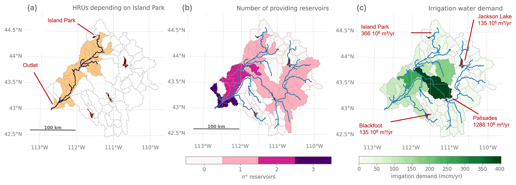
Figure 1Illustration of the irrigation topology for the Snake River basin (with the basin outlet taken at American Falls reservoir, ID, USA). Selection of river segments and corresponding downstream HRUs of the Island Park reservoir (a), number of reservoirs supplying water to each HRU (b), and total irrigation water demand per HRU and reservoir calculated using the irrigation topology (c). Reservoir locations are taken from GRanD, the river network from HDMA, and the irrigation demand is remapped from a gridded CLM simulation (see Sect. 3.2).
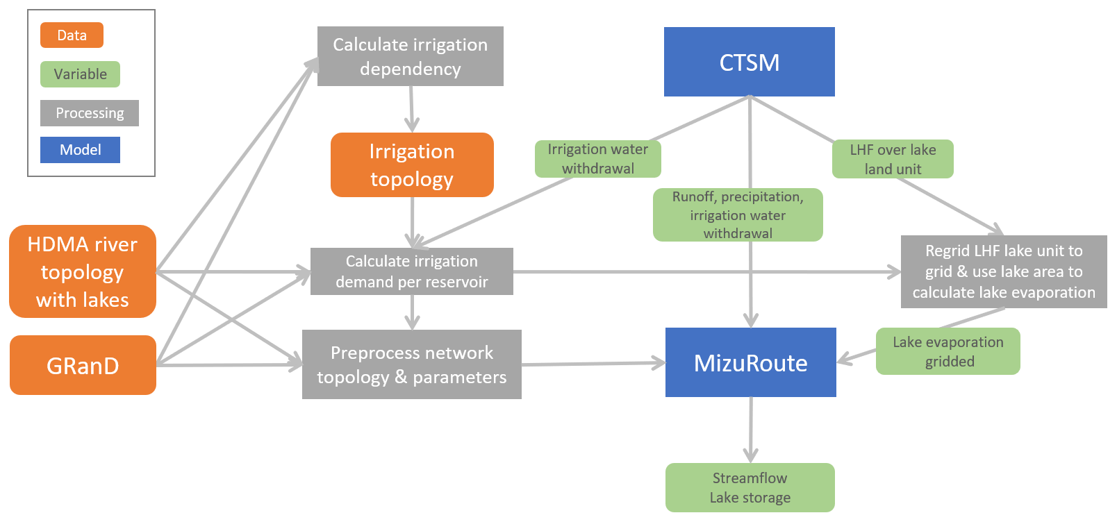
Figure 2Schematic representation of the modelling workflow for the global-scale mizuRoute application using input data and parameters based on Community Land Model (CLM) simulations. LHF refers to latent heat flux.
The lake and reservoir parameterizations in mizuRoute are evaluated in both local and global settings. By using observed streamflow values as forcing, the local mizuRoute application allows for direct evaluation of the implementation of the different outflow schemes. In the global-scale mizuRoute application, outlined in Fig. 2, the reservoir schemes are embedded in global-scale routing simulations that receive forcing fields directly from the land model.
3.1 River network topology
The Hydrologic Derivatives for Modelling and Applications (HDMA; Verdin, 2017) is a vector-based river network based on HydroSHEDS, GMTED2010, and SRTM digital elevation models (DEMs) and entails 295 335 river reaches and HRUs with a scale of 250 km2 (the minimum upstream area to define the start of a river reach). Lakes are included on the HDMA river network by geo-referencing lake polygons of the HydroLAKES dataset (Messager et al., 2016) with a surface area larger than 10 km2 compared to their corresponding river reaches (Gharari et al., 2022). The lake polygons from the HydroLAKES dataset are linked to the Global Reservoir and Dam dataset (GRanD; Lehner et al., 2011), which provides additional information about reservoirs including maximum reservoir capacity and reservoir purpose. Based on this information, a lake segment is classified as a reservoir if it is present in GRanD (including both constructed reservoirs and dam-controlled lakes). Of the 7250 reservoirs available in GRanD, 1773 are included in the river network based on the corresponding polygon from HydroLAKES that are resolved on the river network, of which 484 are categorized as irrigation reservoirs. Likewise, every reservoir is resolved individually on the river network.
3.2 Land model forcing
We conducted a global land-only simulation with the Community Land Model (CLM; Lawrence et al., 2019) that receives prescribed meteorological conditions from the Global Soil Wetness Project (GSWP3; http://hydro.iis.u-tokyo.ac.jp/GSWP3/, last access: 19 May 2022; see also Lawrence et al., 2019) and prescribed vegetation phenology from MODIS (IHistClm5SP component set). The simulation is run on a 0.5∘ by 0.5∘ grid for the period 1961–2015 (including 5 years for spin-up). The simulation is conducted with the updated lake and reservoir mask based on HydroLAKES and GRanD as described in Vanderkelen et al. (2021) and the default irrigation algorithm, without constraints on water availability. Therefore, simulated grid cell irrigation water withdrawal corresponds to the total irrigation water demand of the grid cell. The daily simulated gridded runoff is directly used as input to mizuRoute and remapped to the river network catchments using the first-order conservative remapping method within mizuRoute. Furthermore, the precipitation and evaporation over lakes and reservoirs, necessary for their water balance, are also provided by CLM and remapped to the individual reservoir segments within mizuRoute. Precipitation is directly provided, while lake evaporation is calculated in an intermediate processing step, i.e. by converting the latent heat flux at the lake “land unit” level to evaporation using the latent heat of vaporization (2.501×10⁶ J kg−1).
3.3 Parameters of the outflow parameterizations
All parameters required for the lake and reservoir schemes are provided through the network topology (Appendix Table A1). Maximum reservoir capacity and the reservoir purpose are both provided by the attributes from GRanD. Only the reservoirs for which GRanD assigns irrigation as the main purpose are categorized as irrigation reservoirs in mizuRoute. At the start of the simulation, the initial storage is set at the maximal storage capacity. In the local mizuRoute simulations, monthly mean inflow values are calculated based on observed inflows according to their availability (Appendix Table A1). For the global-scale mizuRoute simulations, monthly mean inflow values per reservoir are obtained from a mizuRoute simulation with only natural lakes using the Döll et al. (2003) parametrization for the period 1979–2000. For both the local- and global-scale simulations, mean monthly irrigation water demands per reservoir are calculated based on the gridded CLM simulation for the same period. The gridded demands are first remapped to the HRUs of the vector-based river network, and the irrigation topology described in Sect. 2.3 is subsequently applied using dependency thresholds of 700 km (maximum downstream distance along the main river stem) and 100 km (maximum distance along tributaries from the main river stem).
3.4 The mizuRoute simulations
In the first step, local mizuRoute simulations are conducted for 26 individual reservoirs using observed reservoir inflows as input forcing (Sect. 4.1, Appendix Table A2). Reservoir outflow is either modelled as a natural lake with the Döll et al. (2003) parametrization (hereafter denoted as NAT), as a human-operated reservoir with the Hanasaki et al. (2006) parametrization (DAM), or as run of the river assuming there is no reservoir using observed inflow as outflow (NOLAKES). To evaluate the use of the Hanasaki et al. (2006) parametrization for irrigation reservoirs in particular, additional simulations are conducted with all reservoirs considered as non-irrigation reservoirs (DAM_NOIRR). Simulations are performed at a daily time step but are compared to observations according to the observational time steps (daily for 18 reservoirs and monthly for 8 reservoirs).
In the second step, four global-scale mizuRoute simulations are conducted on a daily time step using the HDMA river network topology, gridded runoff from CLM, and the IRF-UH routing method. Similar to the local simulations, four simulation types are performed. The first uses the Döll et al. (2003) parametrization for all reservoirs and lakes on the river network (NAT). The second simulation (DAM) uses the parametrization of Hanasaki et al. (2006) for reservoirs and dam-controlled lakes, in addition to Döll et al. (2003) for the natural lakes. Third, all lakes and reservoirs are treated as normal river segments (NOLAKES). Finally, an additional simulation is performed, similar to DAM but with all reservoirs considered as non-irrigation reservoirs (DAM_NOIRR). Comparing this simulation to the DAM simulation allows us to assess the added value of accounting for irrigation water demand using our irrigation topology. Every simulation is conducted for the period 1979–2000, of which the first 2 years are considered spin-up and are excluded from the analysis.
Both local- and global-scale mizuRoute simulations are evaluated with observations of individual reservoirs. In addition, the global-scale mizuRoute simulations are compared to global streamflow indices.
4.1 Local reservoir observations
Observations for reservoir inflow, outflow, and storage are retrieved from the dataset of Yassin et al. (2019), including information on 37 reservoirs worldwide assembled from different sources. We use a subset of 26 reservoirs from this dataset, corresponding to the reservoirs that could be located on the HDMA river network, and they are thus modelled in our mizuRoute simulations (Table A2). Due to data availability, these reservoir observations are not evenly distributed over the globe (Fig. 6). The dataset provides daily inflow, storage, and outflow observations for 18 reservoirs and monthly observations for the remaining 6 reservoirs. To evaluate the global mizuRoute simulations, we complement the reservoir observations from Yassin et al. (2019) with the ResOpsUS historical reservoir dataset for the contiguous United States (CONUS) (Steyaert et al., 2022). Of the 679 reservoirs in the dataset, we use a subset of 32 reservoirs for which both outflow and storage observations are available within the simulation period and that are resolved on the employed HDMA river network.
4.2 Observations from the Global Streamflow Indices and Metadata (GSIM) archive
The Global Streamflow Indices and Metadata archive (GSIM) is a worldwide collection of indices derived from more than 35 000 daily streamflow time series (Do et al., 2018a). The dataset provides quality-controlled time series indices on yearly, seasonal, and monthly resolution compiled from 12 databases with daily streamflow, including both research databases and national databases (Do et al., 2018a; Gudmundsson et al., 2018). Here, we use the following indices, all on a monthly timescale: mean daily streamflow (MEAN; m3 s−1), standard deviation of daily streamflow (SD; m3 s−1), and the minimum and maximum daily streamflow (MIN and MAX, m3 s−1). We only use stations that are located on the river network based on the coordinates of the stations. First, the stations with suspect coordinates are excluded. Second, we select all stations with observation periods overlapping the simulations period (1981–2000) and within a 0.002∘ spatial error tolerance limit on the river network (10 233 stations). Finally, only stations less than 200 km downstream of a simulated reservoir are kept. This is results in 406 GSIM stations used in the analysis.
4.3 Global G-RUN runoff reconstructions
We evaluate CLM runoff using the global runoff reconstruction from the G-RUN ENSEMBLE (Ghiggi et al., 2019, 2021b). G-RUN provides monthly runoff rates on a 0.5∘ grid for 1971–2010 based on upscaled river discharge using a machine learning algorithm (Ghiggi et al., 2019). The G-RUN ENSEMBLE extends the original G-RUN based on GSWP3 with 21 different atmospheric datasets (Ghiggi et al., 2021b). In this study, we use the ensemble mean averaged for 1971–2000.
4.4 Evaluation metrics
Simulated time series are compared to observations for their corresponding periods using the Kling–Gupta efficiency (KGE; Gupta et al., 2009) and the absolute percent bias (PBIAS; Eq. 6).
where n is the number of observations and m and o are the simulated and observed series, respectively. To investigate the role of the different components, we use the KGE following Eq. (7; Gupta et al., 2009).
where r is the linear correlation between simulated and observed values, is the ratio of modelled and observed standard deviation representing the variability error, and is the ratio of the modelled and observed means representing the mean bias. Following Knoben et al. (2019), KGE values above −0.41 are considered better model performance compared to the mean flow benchmark.

Figure 3Evaluation using Kling–Gupta efficiency (KGE) of the Hanasaki et al. (2006, DAM) and Döll et al. (2003, NAT) parameterizations with observed inflows, and evaluation using inflow as outflow (assuming there is no lake, NOLAKE) against observed outflow (a) and observed storage (b) using observations from Yassin et al. (2019). The reservoirs are ordered from low to high capacity ratio, defined as the ratio between the mean annual inflow and storage capacity (see Table A2).
5.1 Local mizuRoute simulations
The local mizuRoute simulations with observed daily reservoir inflows enable directly comparing the different outflow parameterizations and run of the river conditions (Fig. 3). For outflow, the DAM simulation produces the highest KGE scores for 12 of 26 reservoirs (Fig. 3a), while the NAT simulation performs best for 8 reservoirs. The NOLAKES simulation typically yields good skill for reservoirs with a low capacity ratio, where outflows are strongly influenced by inflow seasonality as their storage capacity is small compared to the annual mean inflow (upper half of Fig. 3a, Appendix Figs. A2 and A3). For all simulations, the performance of simulated outflow decreases with increasing reservoir capacity ratio (apart from a few exceptions).
For storage, the DAM simulation outperforms NAT for most reservoirs (18 out of 26; Fig. 3b, Appendix Figs. A2 and A3), with a median KGE of 0.4 compared to 0.08. Especially for reservoirs with a high capacity ratio, DAM shows notably higher KGE values compared to NAT. This demonstrates the added value of the Hanasaki et al. (2006) parametrization in minimizing the inter-annual outflow variability for reservoirs with a high capacity ratio. The individual time series of modelled storage show systematic overestimation and underestimation for the Glen Canyon, Amistad, and Navajo reservoirs, with excessive outflow values indicating the reservoir reached its maximum capacity (Appendix Figs. A2 and A3). In our modelling workflow, the maximum storage capacity is provided by GRanD for all reservoirs on the river network, and therefore these systematic storage biases may be caused by discrepancies between the real reservoir capacity and those reported in GRanD (e.g. for the Navajo reservoir, GRanD reports a maximum capacity of 1278×106 m3, while the US Board of Reclamation reports a capacity of 2107×106 m3, which better corresponds to the observations).
The comparison of the DAM with the DAM_NOIRR simulations for irrigation reservoirs reveals that accounting for irrigation only has a limited effect in the current implementation, except for at the Oldman, St. Mary, Nurek, Sirikit, and Bhumibol reservoirs, where accounting for irrigation demands improves the outflow simulation (Appendix Figs. A1 and A2). For example, Bhumibol and Sirikit are multi-year irrigation reservoirs with a clear irrigation signature in their observed outflow seasonality, as they buffer water during the high-flow season to release for irrigation during the low-flow season (Hanasaki et al., 2006). The simulated annual outflow cycle for the Sirikit reservoir shows slightly increased outflows during the low-flow season (February–May) for the original Hanasaki parametrization compared to Hanasaki without irrigation demands (Fig. A2). The limited added value of accounting for irrigation demands for the 12 irrigation reservoirs suggests that reservoir irrigation demands are likely underestimated in this modelling framework (see Sect. 6.2).
5.2 Global-scale mizuRoute simulations: evaluation with reservoir observations
The evaluation using the Yassin et al. (2019) dataset shows that the global-scale mizuRoute simulations are substantially worse overall than the simulations using observed inflows, with median KGE values for outflow of −0.29, −0.29, and −0.35 for the DAM, NAT, and NOLAKES simulations, respectively (Fig. 4b). Most reservoirs have negative KGE scores, and for 4 out of 26 reservoirs all simulations are outperformed by the mean annual flow benchmark. In terms of percent absolute bias for outflow, the difference between the DAM and NAT is very small or negligible for more than half of the reservoirs (Fig. 4a). This is also visible in the small differences between simulations in the bias term of KGE, in particular for DAM and NAT (Fig. A4b). For correlation, the NAT simulation has the best skill for 15 of 21 reservoirs, with the highest correlations found for reservoirs with low capacity ratios (Fig. A4c). The added value of using the Hanasaki et al. (2006) parametrization for reservoir storage is less apparent in the global-domain mizuRoute simulation, as the DAM simulation outperforms the NAT simulation for 10 of the 21 reservoirs for absolute percent bias and KGE (Fig. 5). Consistent with the observation-driven local simulations, the global-domain DAM simulation performs systematically better for reservoirs with a high capacity ratio and better than NAT in most cases. These findings are generally confirmed by the evaluation with the ResOpsUS reservoir observations, where the DAM outperforms the NAT simulation for 13 of the 32 reservoirs (Fig. A5).
While in the local mizuRoute application the DAM simulation outperforms the NAT and NOLAKES simulations for most reservoirs, especially for storage, this is not the case in the global-domain mizuRoute simulations. The main cause for these discrepancies are biases in the simulated reservoir inflow, which could be originating from biases in the simulated runoff from CLM or from small reservoirs upstream and their dam operations, which are not resolved in the HDMA river network, with the resultant streamflow alterations not included in the river flow. For 15 of the 21 reservoirs in the dataset, however, there is at least one upstream reservoir resolved in the HDMA river network, as only 6 reservoirs have no upstream reservoir resolved (Trinity, Navajo, Oldman, Seminoe, Sirikit, and St. Mary). The same pattern is found when comparing simulated storage to the observed storage from the ResOpsUS dataset (Fig. A6). The next section therefore focuses on the biases in simulated inflow and runoff.
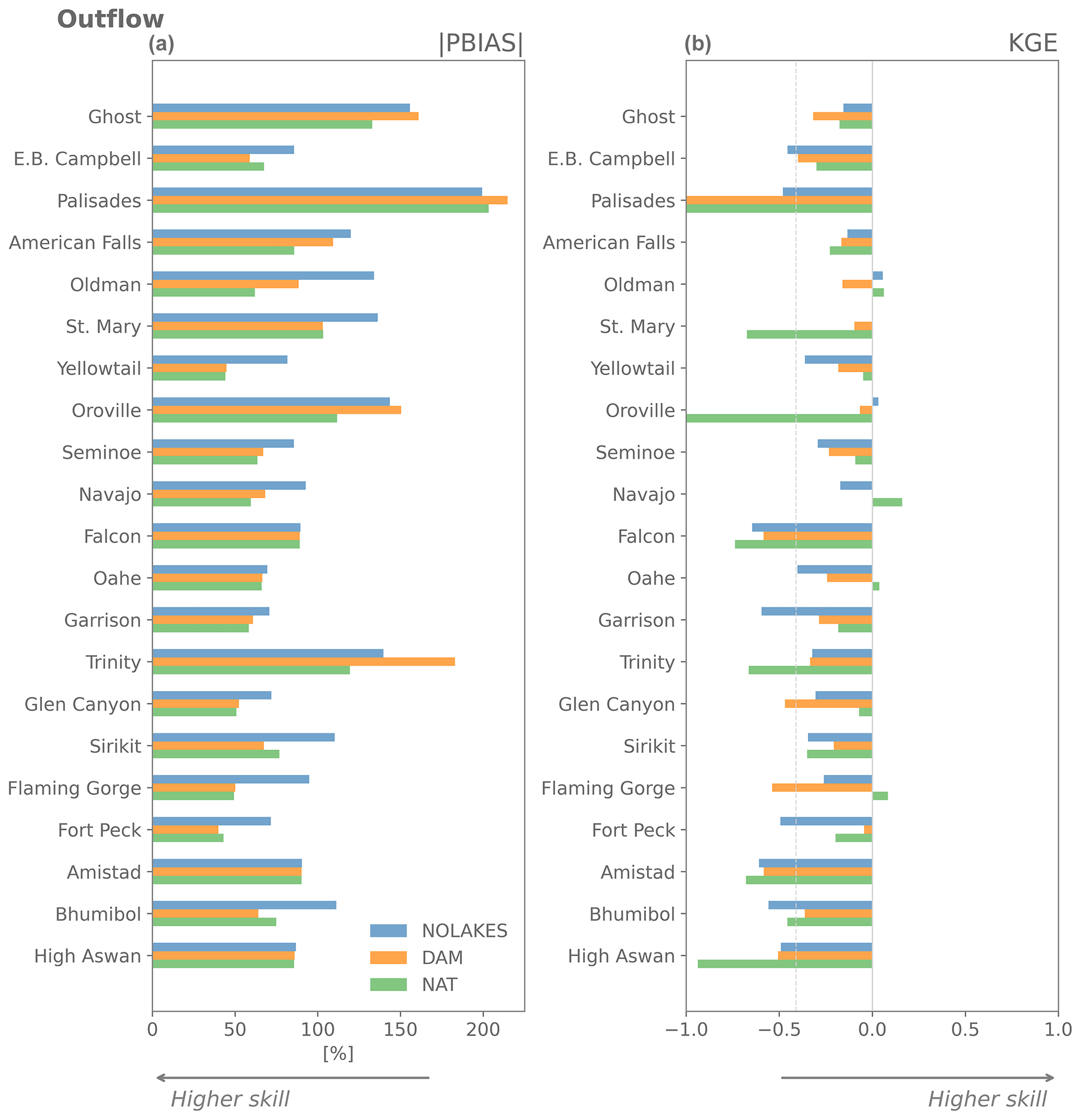
Figure 4Performance of the global-domain mizuRoute simulations for outflow compared to reservoir observations using absolute percent bias (|PBIAS|, a) and Kling–Gupta efficiency (KGE, b).

Figure 5Performance of the global-scale mizuRoute simulations for storage compared to reservoir observations using the absolute percent bias (|PBIAS|, a) and Kling–Gupta efficiency (KGE, b).
5.3 Inflow and runoff bias of CLM forcing
The comparison of simulated spatially distributed runoff from CLM with the global reconstructions of G-RUN reveals substantial biases (Fig. 6). The mean annual runoff bias is +0.077 mm d−1, but regionally large differences exist: runoff is overestimated in northwestern Amazonia, western Africa, large parts of China, western India, Japan, and to a lesser extent in the central US and the European mainland. CLM underestimates runoff in the tropical rainforest areas of central Amazonia and the Congo basin and in mountain areas, like the Pakistani mountain ranges, the European Alps, the Rocky Mountains in the US and Canada, the northern part of the Andes, and the Southern Alps in New Zealand.
As 20 reservoirs in the dataset are located in the central and western parts of the contiguous United States and Canada, we focus on these regions to compare runoff and reservoir inflow seasonality to observations (Fig. 7). In the plains, runoff is generally slightly overestimated, while in the mountainous areas like the Rocky Mountains, Sierra Nevada, and Cascade Range mean annual runoff is substantially underestimated (Fig. 7a). Via flow routing, these runoff biases translate into streamflow biases (Fig. 7b–s).
Overall, the simulated streamflow deviates from the observed seasonal cycles in terms of absolute bias, timing of the high flows, and amplitude. The deviations can thereby roughly be grouped into four categories of reservoirs. First, for large reservoirs like Amistad and Falcon International on the Rio Grande and Garrison and Oahe on the Missouri River (Fig. 7h–k), mizuRoute (forced with CLM output) largely overestimates the observed inflows (up to +1434 % for Falcon). For these reservoirs the upstream flows are highly regulated by dam operations and the positive inflow biases are therefore likely originating from unrepresented upstream dam operations (Shin et al., 2019) or from positive biases in simulated runoff (see discussion Sect. 6.1). Other reservoirs have inflows highly controlled by snowmelt, with their headwaters in the Rocky Mountains (Flaming Gorge, Navajo, Palisades, American Falls, and Glen Canyon reservoirs; Fig. 7n, l, r, q, m). For most of these reservoirs, the annual peak in inflow, likely coming from snowmelt, is simulated 2–3 months too early (March–April–May) compared to the peak in observed inflows (June–July–August). This is also the case for the small within-a-year reservoirs in the Canadian Rocky Mountains (Oldman, St. Mary, and Ghost reservoirs; Fig. 7b, c, s). These biases in runoff timing could potentially be related to unresolved topography in these coarse-resolution simulations. For the mainly rain-fed Oroville and Trinity reservoirs (Fig. 7o, p), the release period is simulated too early in the year. Finally, some Canadian reservoirs, like the E.B. Campbell reservoir, show only little variation in storage, which could in part be explained by the linkages of these reservoirs with lake and swamp systems.
These inflow discrepancies point at deficiencies in the simulated runoff, as the comparison of spatially aggregated runoff from CLM versus G-RUN over the reservoir catchments show similar patterns (not shown). Moreover, local systematic biases in runoff are aggregated over the catchment and result in magnified inflow biases. Previous research showed that the runoff inputs are a more important bias source for river discharge in mizuRoute compared to the river network and routing scheme when analysed on monthly time steps (Mizukami et al., 2021). In other large-scale hydrological models, annual river discharge shows broad range of values, and there are also large differences between runoff ratios among different models (Masaki et al., 2017; Haddeland et al., 2011).
The inflow biases are adversely affecting the skill of the reservoir parametrization in the global-domain mizuRoute simulations compared to the local applications, especially for reservoir storage. We therefore anticipate that when the runoff simulations are improved within the driving land model, in this case CLM, improved results can be expected also in global-scale mizuRoute simulations. Therefore, we focus on comparing the DAM simulation to the NOLAKES simulation in the remainder of this paper.
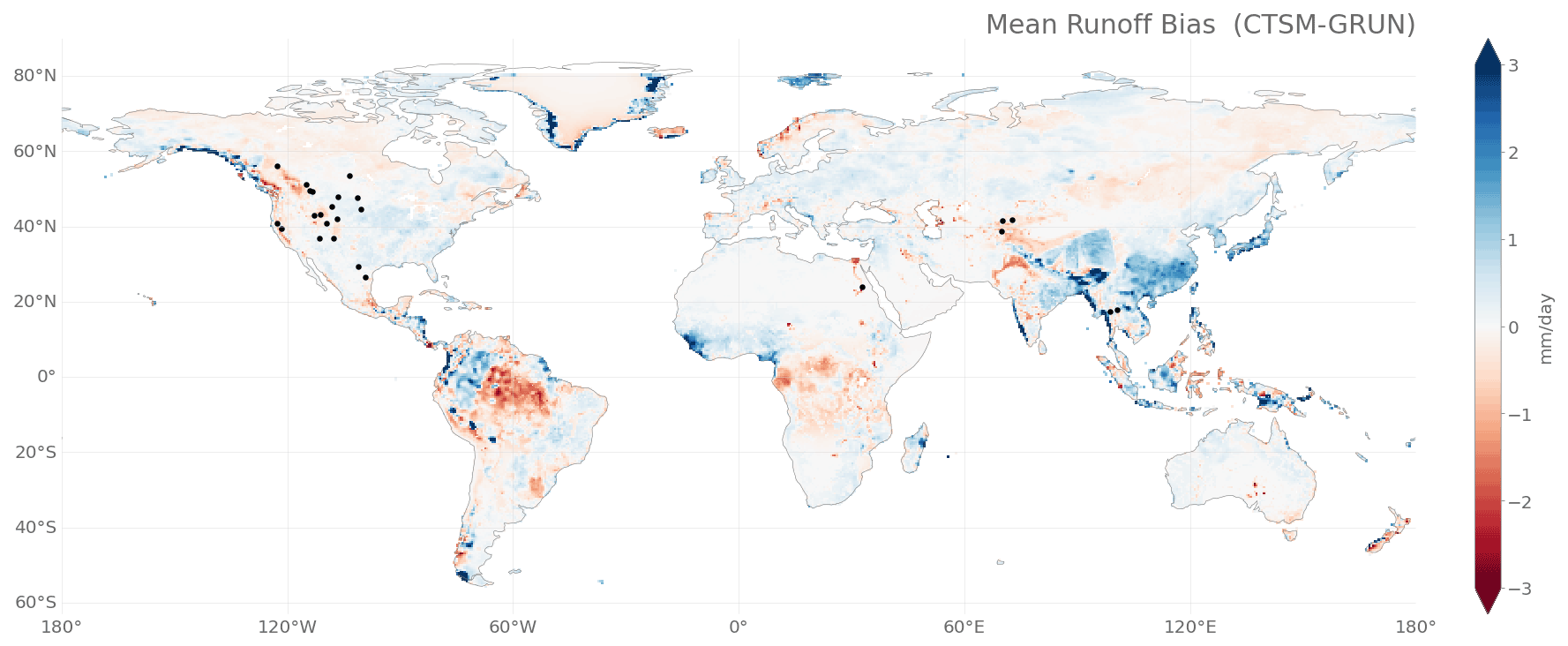
Figure 6Mean runoff bias of CLM compared to G-RUN for the period 1971–2000. Black circles indicate the reservoirs used from the Yassin et al. (2019) dataset.
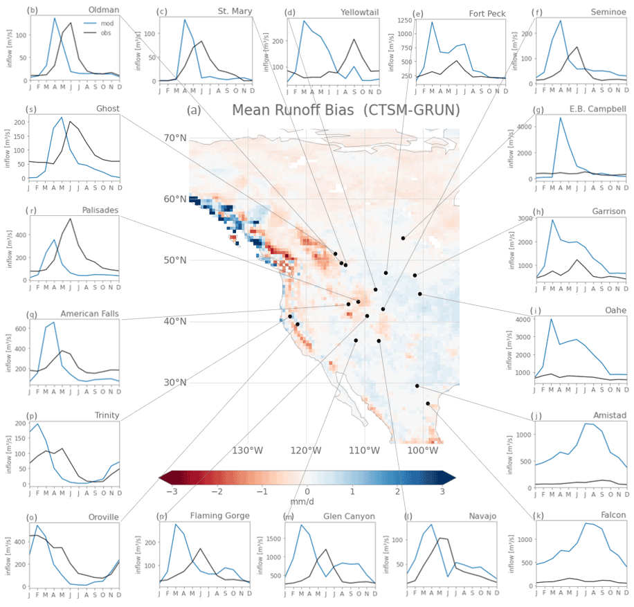
Figure 7Mean runoff bias of CLM compared to G-RUN for CONUS and Canada with location of reservoirs (a). Simulated (blue line) and observed inflow (black line) seasonality per reservoir (b–s).
5.4 Global-scale mizuRoute simulations: evaluation for global streamflow indices
We evaluate the global impact of accounting for dam operations on long-term river discharge by comparing the skill of the DAM with the NOLAKES simulation for observed monthly streamflow indices from the GSIM archive (Fig. 8). In general, the DAM simulation shows improved skill compared to the NOLAKES simulation (Fig. 8e–h), with a median absolute percent bias for mean flows of 72 % compared to 81 %. The improvement is particularly strong for the standard deviation, with a mean absolute percent bias of 187 % for NOLAKES compared to 100 % for DAM, indicating an improvement of the total streamflow variability (Fig. 8b). This is not surprising, as reservoir operations typically minimize streamflow variability (Hanasaki et al., 2006). For high floods, the DAM simulation outperforms NOLAKES (79 % compared to 114 % mean absolute bias), with the best improvements in Canada, the western United States, and central Africa (Fig. 8c). Finally, for low floods, the overall improvement is smaller, with a mean absolute bias of 79 % for DAM compared to 91 % for NOLAKES, with the latter providing remarkably better results in India and southwestern USA.
Comparing the DAM and NAT simulations, it is remarkable that NAT shows the best skill for monthly standard deviation (Fig. 8b and Appendix Fig. A8c), which could point at a better buffering of the biased river streamflow by the natural lake scheme of Döll et al. (2003). This corresponds to the findings of the global-scale mizuRoute evaluation to individual reservoirs observations (Sect. 5.2). As the Hanasaki et al. (2006) parametrization mainly depends on mean annual and monthly inflows, it suffers from the inflow biases, while the natural lake parametrization of Döll et al. (2003) mainly attenuates the incoming inflow. In India and the southeastern US, daily low flows are better represented in the NOLAKES simulation (Fig. 8d). Overall, the difference between NAT and DAM is small compared to the difference between not representing lakes and representing lakes. On average, NAT is outperforming DAM for the mean, standard deviation and monthly maximum indices. For low flows, however, DAM shows the best performance, with a median absolute percent bias of 90 % for the NAT simulation compared to 79 % for DAM (Fig. 8h). The DAM simulation shows substantially higher skill in representing low flows, especially in India and southern Africa (Appendix Fig. A8d).
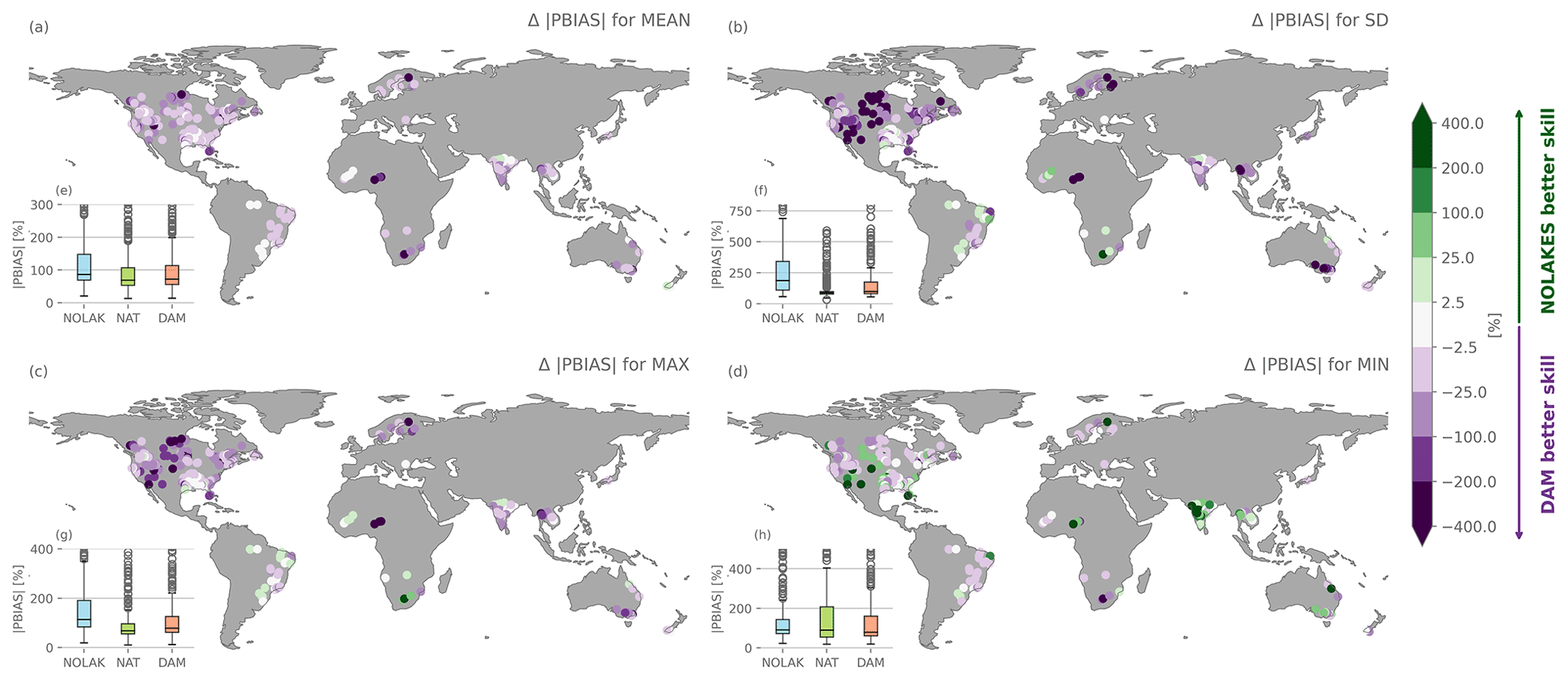
Figure 8Performance of global-scale mizuRoute simulations for streamflow indices of GSIM. Added value in absolute percent bias of accounting for reservoirs (DAM) over simulations without lakes or reservoirs (NOLAKES) (|PBIAS|DAM − |PBIAS|NOLAKES) for monthly mean streamflow (MEAN, a), monthly streamflow standard deviation (SD, b), monthly maximum streamflow (MAX, c) and monthly minimum streamflow (MIN, d). Note the non-linear colour bar scale. Inset panels (e)–(h) show the |PBIAS| for the simulation without lakes (NOLAKE), with only natural lakes (NAT), and accounting for reservoirs (DAM). Only GSIM stations on the river network, a maximum 200 km2 downstream of a reservoir, and with observations in the simulation period are included.
6.1 Reservoir parametrization and river network
The deterioration in skill of the Hanasaki et al. (2006) parametrization relative to natural lakes when using simulated inflow indicates a larger sensitivity of the Hanasaki et al. (2006) scheme to inflow magnitude and timing, which exacerbates the bias. The parametrization of Hanasaki et al. (2006) is designed to provide generic operational rules, rather than observation-driven release rules for individual reservoirs (Turner et al., 2020). These generic rules likely exacerbate bias at some of the reservoirs. However, individual calibration could improve simulated releases of modelled reservoirs. Especially for highly regulated rivers with a series of cascading reservoirs, calibration schemes of upstream reservoir releases could improve the modelled river streamflow (Shin et al., 2019). However, prior to conducting such parameter calibration, it would be advisable to first reduce biases in the reservoir inflows as simulated by CLM (Sect. 6.3).
The overestimated inflow for reservoirs with highly regulated upstream flows, like Amistad and Falcon International reservoirs on the Rio Grande (Fig. 7j and k), is likely due to unresolved reservoirs upstream. For example, only 6 of the 23 dams and water diversions on the Rio Grande are resolved within the current river network, which could be attributed to the following reasons. First, cascade systems and run-of-river dam infrastructure styles (e.g. Leasburg and Isleta dams on the Rio Grande), which control the river flow but do not store water, are generally not included in GRanD and are therefore not in the river network. Second, several dams and associated reservoirs are not on the stream network due to the network resolution (e.g. the remote Platoro reservoir on the Conejos River). Third, reservoirs smaller than the area threshold of 10 km2 are not included on the river network (e.g. Sumner reservoir).
These issues could be accommodated by the use of higher-resolution stream networks on which more reservoirs would be resolved, like the Multi-Error-Removed-Improved-Terrain (MERIT) hydro network, which is derived from a global DEM at 3 arcsec resolution (∼90 m; Yamazaki et al., 2019). An accurate high-resolution DEM is important to improve the reservoir representation and release, as has been shown by Shin et al. (2019). The choice of river network proves, however, to be less important compared to the runoff input from the land model for global-scale river flow simulations without lakes and reservoirs (Mizukami et al., 2021), so accounting for and reducing runoff biases remains an essential step. Finally, to account for run-of-river dams, the GRanD database could be updated or complemented by other data sources like the Global Georeferenced Database of Dams (GOODD; Mulligan et al., 2020).
The parametrization of Hanasaki et al. (2006) is designed to provide generic operational rules, rather than observation-driven release rules for individual reservoirs (Yassin et al., 2019; Turner et al., 2020). In a recent study for CONUS and Canada, Turner et al. (2021) showed that empirically derived reservoir operating rules based on historical reservoir operations significantly improve release and storage simulations compared to the Hanasaki et al. (2006) scheme, even when extrapolated to similar reservoirs without historical records available. While such an approach provides promising results, it is only tested with observed reservoir inflows, and limited to regions where data-rich reservoirs can be representative for the operation rules and hydrological conditions of data-scarce reservoirs. In a coupled framework, the method would still propagate the inflow biases coming from the driving model but might have improved storage representation due to the targeted operation range (Turner et al., 2021). In the context of ESMs and future projections, however, generic methods allow for the incorporation of future climate changes and their impacts on the river flows and irrigation demands on a global scale.
6.2 Irrigation demand and topology
The local mizuRoute simulations showed only small differences in outflow values for the DAM and DAM_NOIRRIG simulations for irrigation reservoirs. Our results suggest that the total irrigation water demand per reservoir is underestimated and that there are also potential biases in the irrigation seasonal cycle. These uncertainties are either originating from the irrigation topology, defining the area to which the reservoir water is allocated, or from the gridded irrigation amounts simulated by CLM. Since applying the irrigation topology with different thresholds (1000 km instead of 700 km downstream along the main river stem and 200 km instead of 100 km along the tributaries) did not significantly improve the irrigation demands, disparities in simulated irrigation amounts likely play a major role.
The irrigation module in CLM is calibrated with one free parameter based on global observed irrigation water withdrawals from AQUASTAT (Thiery et al., 2017, 2020). It is, however, possible that these country-based irrigation amounts are under-reported by individual countries. In addition, while global crop calendar data exists to a limited extent (e.g. Sacks et al., 2010), there is almost no information on timing and amount of global irrigation water withdrawals to use for model evaluation. However, there are various possible pathways to improve the simulation of irrigation water withdrawal, like differentiating irrigation techniques applied in different regions around the world (Jägermeyr et al., 2015) and including crop rotation and other agricultural management practices (e.g. Hirsch et al., 2017, 2018). Furthermore, the use of remotely sensed soil moisture to estimate the amount and timing of irrigation demonstrates promising results (Brocca et al., 2018; Zaussinger et al., 2019; Massari et al., 2021; Lawston et al., 2017). Future improvements in the irrigation module of CLM will likely lead to improvements in the simulated reservoir storage and release.
Apart from the uncertainties in gridded irrigation demands from CLM, there are several opportunities to improve the irrigation topology routine. Here, we use the HDMA river network topology and determine the HRUs contributing to reservoir water demand using simple rules based on distance and bottom elevation of river segments. However, more detailed river networks, like MERIT-Hydro (Yamazaki et al., 2019), enable refining the criteria. For example, MERIT-Hydro now includes more topological details such as the height above nearest drainage index (Nobre et al., 2011; Gharari et al., 2011). Future improvements in the irrigation topology could also account for water transfers, including water diversion for irrigation at weirs (Hanasaki et al., 2022).
6.3 Runoff biases in CLM
The inflow biases shown in Sect. 5.3 for the reservoirs in the CONUS and Canada can be roughly subdivided into reservoirs where there is a bias in inflow timing and reservoirs where the inflow is largely overestimated (with some exceptions). In our modelling framework, the biases in inflow timing for reservoirs with mountainous headwaters could originate from the lack of a representation of high-elevation snow pack and the associated timing of snowmelt in these relatively coarse-resolution simulations. Another potential source of uncertainty is the sensitivity of runoff simulations to the meteorological forcing providing biased timing and amounts of precipitation, especially in high-elevation mountain catchments, which affect the runoff ratios. We tested these hypotheses by running mizuRoute over the North American domain using a high-resolution CLM simulation forced with North American Land Data Assimilation System (NLDAS) meteorological forcing on a high-resolution grid (0.125∘; Appendix Fig. A7). These simulations did not improve magnitude or timing of the inflow biases, and thus it is likely that these uncertainties are coming from CLM's representation of hydrological processes (e.g. the seasonal cycles of snow accumulation and melt). For the large reservoirs with headwaters in the plains like the Falcon International and Amistad reservoirs, a second reason for the large positive inflow biases next to unresolved upstream river regulation is the suspected underestimation of the amount of irrigation water applied (Sect. 6.2). In addition, CLM does not include water abstractions for domestic and industrial purposes (Telteu et al., 2021), which would explain the high bias in simulated streamflow.
There are several potential avenues for future model development that could potentially reduce the model runoff and streamflow errors, especially the timing errors. Natural processes related to snow accumulation and melt dynamics could be investigated and improved. Ongoing work with the new representative hillslope model within CLM, which now includes temperature and precipitation downscaling, as well as the impacts of slope and aspect on hillslope to lateral flow, could potentially help resolve early runoff peak biases (Swenson et al., 2019). Felfelani et al. (2020) have also explored how explicit grid-to-grid lateral flow can improve high-resolution CLM simulations. Additionally, CLM parameters, which have previously been calibrated for evapotranspiration and gross primary production (Dagon et al., 2020), could be calibrated for runoff as well.
6.4 Future work on representing reservoirs in a coupled Earth system model
The modelling framework in this study is an application of the routing scheme mizuRoute and the land model CLM (the land component of CESM), in which both models are employed in standalone mode. Prior to the simulation, mizuRoute remaps the gridded runoff, gridded precipitation, and lake tile evaporation of CLM to the vector-based river network. In addition, the parameters needed for the Hanasaki scheme (Table A1), like mean monthly reservoir inflow and the initial release coefficient, are calculated in an intermediate processing step before being used in the mizuRoute simulation. Finally, the mean monthly irrigation demand per reservoir is calculated using the irrigation topology prior to the mizuRoute simulation.
The coupling of mizuRoute to CLM and CESM will enable us to directly route runoff from the land to the ocean with a network-based routing mode, thereby accounting for streamflow alteration through dam operations. Future work on coupling the vector-based model to the gridded land model will require an on-the-fly remapping step to communicate runoff from the land model to the vector-based river network. As the water balance of natural lakes and reservoirs is simulated within mizuRoute using precipitation and lake evaporation from CLM, the coupling would also enable more realistic lake and reservoir water balance dynamics to the Earth system model, which have not been simulated so far (Gharari et al., 2022; Vanderkelen et al., 2021; Mizukami et al., 2021).
In addition to the water fluxes related to the lake and reservoir water balances, mizuRoute will need the gridded irrigation water demand from CLM, which can be aggregated to individual reservoirs using the irrigation topology. In a one-way coupling, mizuRoute will use this irrigation demand seasonality to determine the dam release for irrigation reservoirs. The two-way coupling of CLM and mizuRoute would ultimately allow for water to be extracted directly from the river for irrigation, thereby using runoff generated in upstream grid cells. In this way, the actual availability of water for irrigation would be better represented. To this end, the irrigation topology could serve as a blueprint for transporting irrigation water across grid cells. Eventually, the coupled system will enable more accurately modelling the human alteration of water resources globally in the present and under different future emission and socioeconomic scenarios.
In this study, we evaluate a reservoir parametrization (Hanasaki et al., 2006) that we integrated into the river-routing model mizuRoute and assess how a simple treatment of human dam regulation affects global streamflow simulations. To this end, we develop an irrigation topology based on the vector-based river network that provides the area over which water demand is aggregated for each individual irrigation reservoir. Local mizuRoute simulations for 26 reservoirs using observed inflows demonstrate that the reservoir parametrization has added value compared to the natural lake scheme of Döll et al. (2003) for the simulation of reservoir release and storage. The reservoir parametrization shows high skill in simulating reservoir storage, particularly for reservoirs with a multi-year storage capacity. The benefits of accounting for irrigation demand seasonality appear to be limited in the existing modelling framework, but this could be either due to a spatial sampling bias of reservoirs with observations available or uncertainties in the simulated irrigation demand.
Biases in modelled river discharge, which can be attributed to runoff biases in CLM, prevent strict validation with observations of the impact from reservoir operations. However, monthly streamflow indices indicate that accounting for lakes and reservoir regulation does appear to improve the representation of mean and high flows as well as flow variability, even if the total amount and timing of runoff is biased.
Our results highlight the opportunities and challenges of global-scale reservoir and streamflow simulations and provide an essential step for representing reservoirs in Earth system models and for incorporating human dam operations in global assessments of water resources availability under present-day and future climates. This enables exploring the role of different reservoir management strategies and priorities in altering water availability under climate change. Moreover, modelling reservoirs in a coupled system will allow us to more accurately evaluate water availability for human consumption, irrigation, and ecosystems, while accounting for interactions between water management, atmospheric processes, and climate change drivers.
Table A1Parameters for the Hanasaki et al. (2006) reservoir parametrization in mizuRoute.
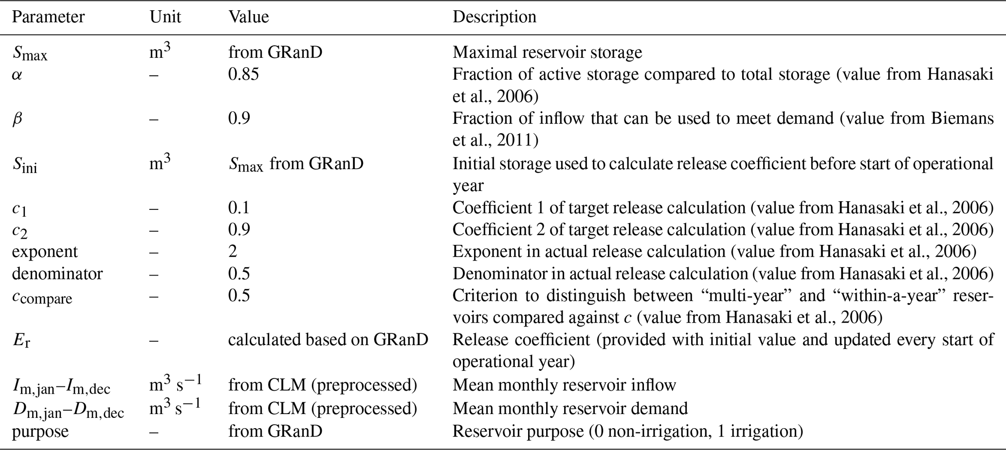
Table A2Reservoirs of the Yassin et al. (2019) observational dataset used in this study. The asterisk in the observation period column indicates this reservoir has monthly instead of daily observations. Maximum capacity is derived from GRanD.
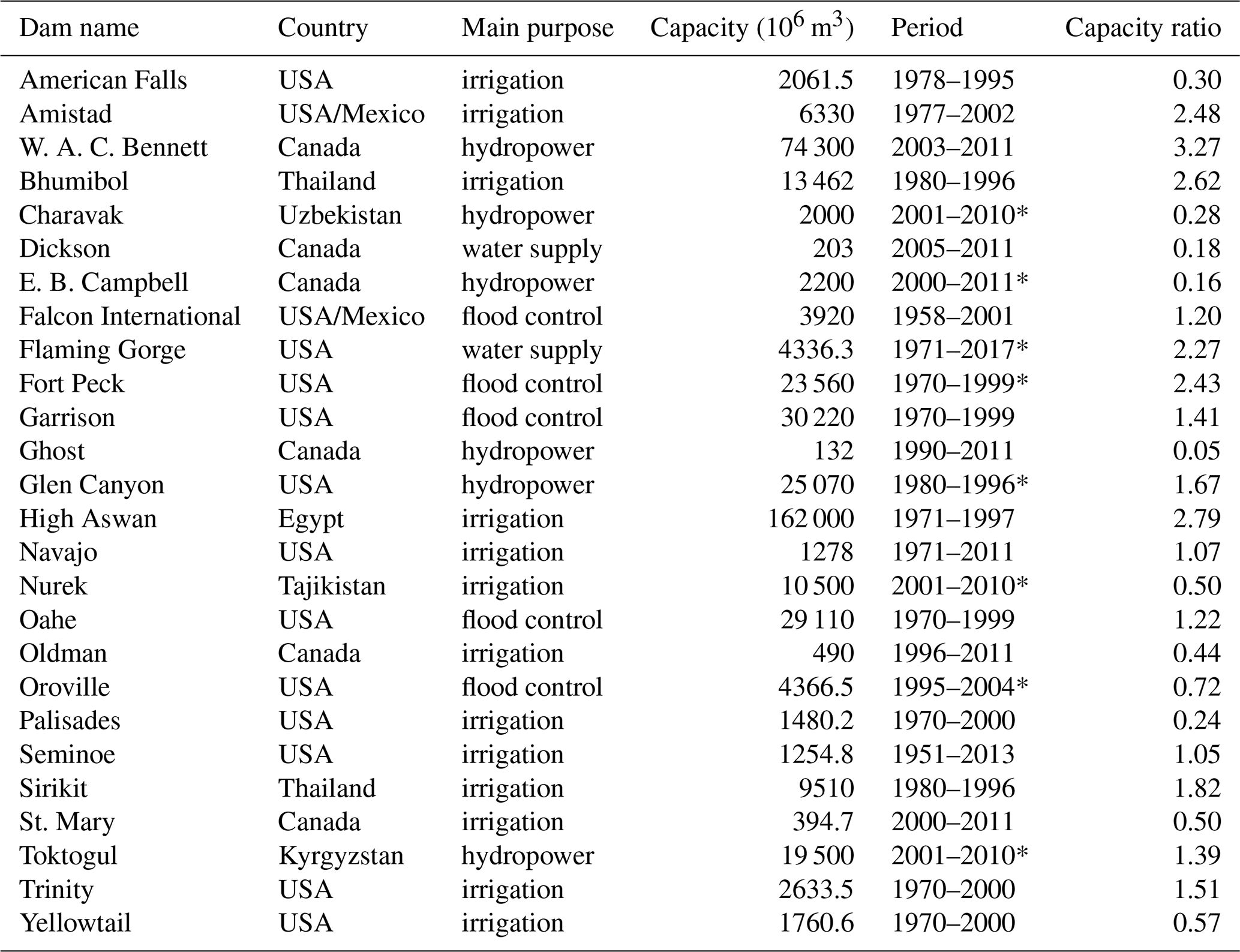
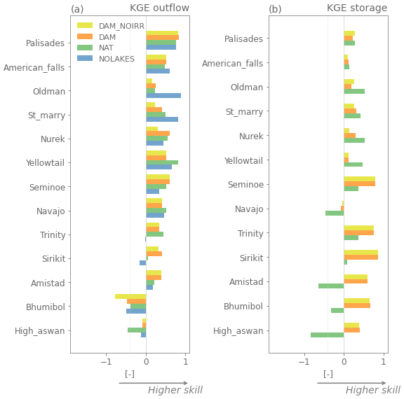
Figure A1Evaluation with Kling–Gupta efficiency (KGE) for irrigation reservoirs of the Hanasaki et al. (2006, DAM) and Döll et al. (2003, NAT) parameterizations with observed inflows and run-of-the-river conditions (assuming there is no lake; NOLAKE) against observed outflow (a) and observed storage (b) using observations from Yassin et al. (2019). The reservoirs are ordered from low to high capacity ratio.
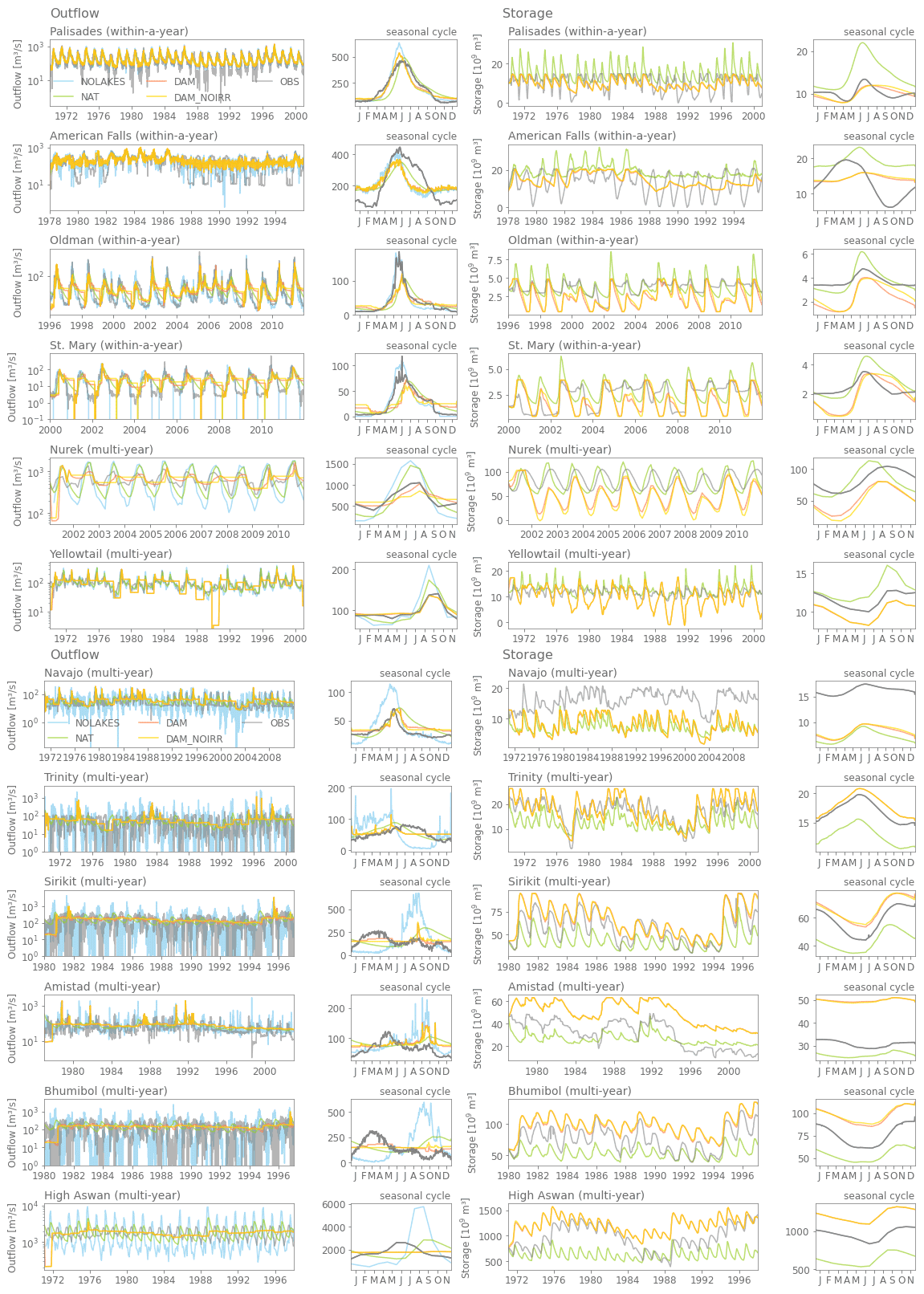
Figure A2Time series and seasonal cycles of outflows and storage of observation driven simulations using the Hanasaki et al. (2006) parametrization with and without accounting for irrigation (DAM and NO_DAM, respectively), the natural lakes Döll et al. (2003) parametrization (NAT), and run-of-the-river conditions (NOLAKES, all for irrigation reservoirs), compared to observations. Note the logarithmic axis for the outflow time series.
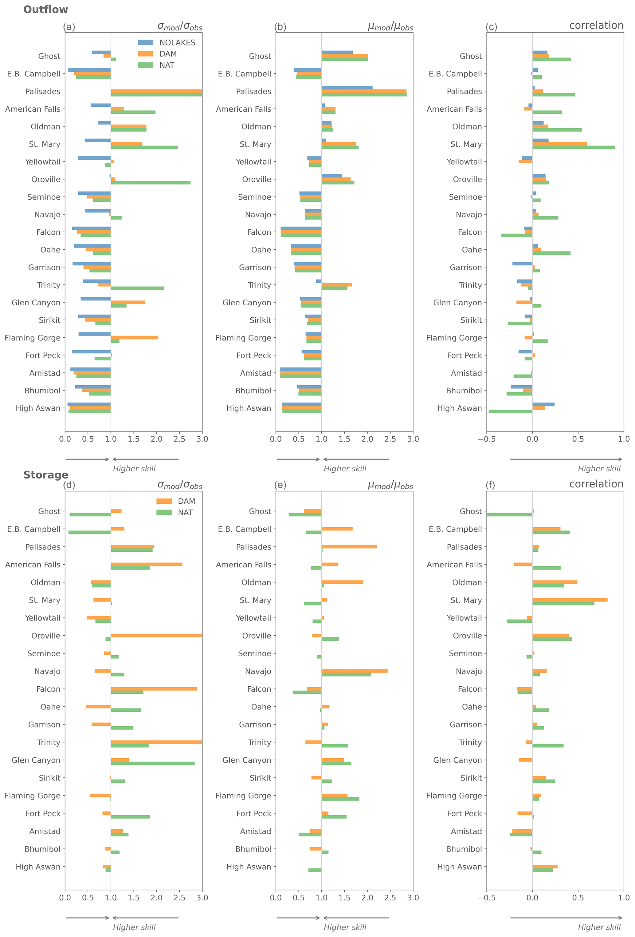
Figure A4Performance for mizuRoute simulations for outflow (a–c) and storage (d–f) compared to reservoir observations using the KGE terms: variability error (, a, c), mean bias (, b, e) and correlation (c, f).

Figure A5Performance of the global-scale mizuRoute simulations for outflow compared to reservoir observations from the ResOpsUs dataset (Steyaert et al., 2022) using absolute percent bias (|PBIAS|, a) and Kling–Gupta efficiency (KGE, b).
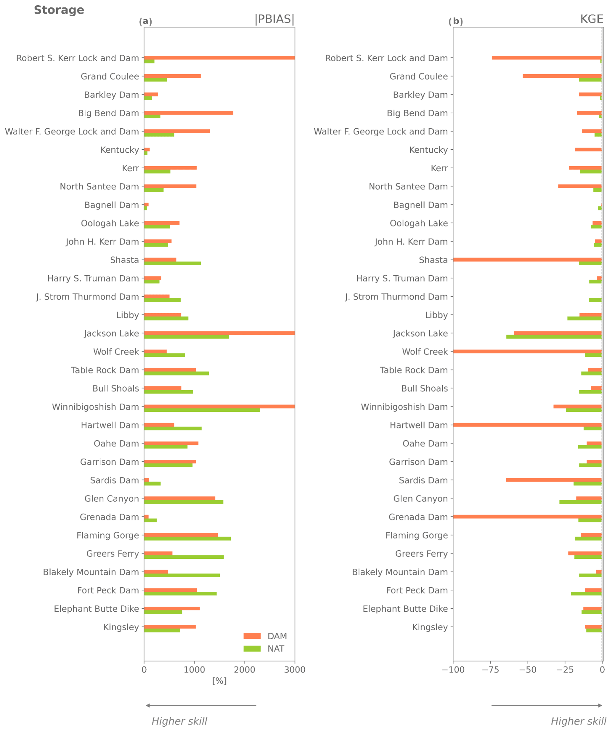
Figure A6Performance of the global-scale mizuRoute simulations for storage compared to reservoir observations from the ResOpsUs dataset (Steyaert et al., 2022) using the absolute percent bias (|PBIAS|, a) and Kling–Gupta efficiency (KGE, b).
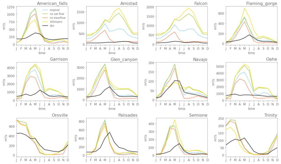
Figure A7Simulated and observed inflow seasonality per reservoir with mizuRoute using runoff from different CLM simulations at 0.125∘ resolution with meteorological forcing from NLDAS. In the legend, “original” refers to the simulation with the default CLM version used in the main analysis, “no sat flow” refers to the simulation where surface saturation excess runoff is set to 0, “no baseflow” refers to the simulation with a decreased baseflow parameter, “hillslopes” refers to the simulation using the hillslope model described in Swenson et al. (2019) and performed at 0.5∘ horizontal resolution, and “obs” are the observed inflows from the Yassin et al. (2019) dataset.
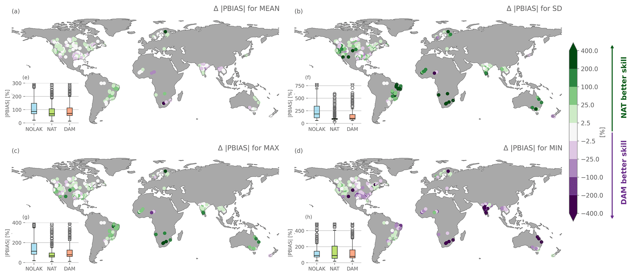
Figure A8The same as Fig. 8 but for the absolute percent bias for natural lakes compared to reservoirs (|PBIAS|DAM − |PBIAS|NAT).
The reservoir dataset described in Yassin et al. (2019) is available at https://doi.org/10.5281/zenodo.1492043 (Yassin, 2018). The GSIM data can be found at https://doi.org/10.1594/PANGAEA.887477 (Do et al., 2018b), while the G-RUN ENSEMBLE reconstructions are available at https://doi.org/10.6084/m9.figshare.12794075 (Ghiggi et al., 2021a). The HydroLAKES dataset is available at https://www.hydrosheds.org/page/hydrolakes (last access: 19 May 2022), GRanD can be found at http://globaldamwatch.org/ (last access: 19 May 2022), and the HDMA dataset can be found at https://doi.org/10.5066/F7S180ZP (Verdin, 2017). The source code of mizuRoute (tag cesm-coupling.n00_v2.0.1) is publicly available at https://github.com/ESCOMP/mizuRoute (last access: 19 May 2022) and https://doi.org/10.5281/zenodo.4395155 (Mizukami et al., 2020), and CLM5.0 is available through the Community Land Model (CLM) repository (https://github.com/ESCOMP/CTSM, last access: 19 May 2022; https://doi.org/10.5281/zenodo.6032448, CTSM Development Team, 2022). The scripts used in this study are available at https://github.com/VUB-HYDR/2022_Vanderkelen_etal_GMD (last access: 19 May 2022), with the following DOI: https://doi.org/10.5281/zenodo.6490979 (Vanderkelen, 2022a). Finally, all input data, ancillary data, and settings used to conduct the mizuRoute simulations used in the analysis are available at https://doi.org/10.6084/m9.figshare.c.5965053.v1 (Vanderkelen, 2022b).
IV, SG, and NM implemented the reservoir parametrization in mizuRoute. IV performed and analysed the simulations. SS, DML, and MPC provided scientific input on CLM and runoff biases. MPC, DML, YP, NH, AvG, and WT provided general oversight and guidance. IV wrote the manuscript with input from all co-authors.
At least one of the (co-)authors is a member of the editorial board of Geoscientific Model Development. The peer-review process was guided by an independent editor, and the authors also have no other competing interests to declare.
Publisher's note: Copernicus Publications remains neutral with regard to jurisdictional claims in published maps and institutional affiliations.
The authors would like to thank Erik Kluzek for his support on CLM. Inne Vanderkelen is a research fellow at the Research Foundation Flanders. Yadu Pokhrel received support from the National Science Foundation (CAREER Award). The CESM project is supported primarily by the National Science Foundation (NSF). This material is based upon work supported by the National Center for Atmospheric Research, which is a major facility sponsored by the NSF under Cooperative Agreement no. 1852977. Computing and data storage resources, including the Cheyenne supercomputer (https://doi.org/10.5065/D6RX99HX), were provided by the Computational and Information Systems Laboratory (CISL) at NCAR. We thank all the scientists, software engineers, and administrators who contributed to the development of CESM2. Other storage resources and services used in this work were provided by the VSC (Flemish Supercomputer Center), funded by the Research Foundation – Flanders (FWO) and the Flemish Government. This study was supported by the LAMACLIMA project, part of AXIS, an ERA-NET initiated by JPI Climate, and funded by BELSPO with co-funding by the European Union.
This research has been supported by the Fonds Wetenschappelijk Onderzoek (grant no. FWOTM920) and the Belgian Federal Science Policy Office (grant nos. B2/181/P1 and 776608).
This paper was edited by Charles Onyutha and reviewed by two anonymous referees.
Biemans, H., Haddeland, I., Kabat, P., Ludwig, F., Hutjes, R. W. A., Heinke, J., Von Bloh, W., and Gerten, D.: Impact of reservoirs on river discharge and irrigation water supply during the 20th century, Water Resour. Res., 47, 1–15, https://doi.org/10.1029/2009WR008929, 2011. a, b, c, d, e, f
Brocca, L., Tarpanelli, A., Filippucci, P., Dorigo, W., Zaussinger, F., Gruber, A., and Fernández-Prieto, D.: How much water is used for irrigation? A new approach exploiting coarse resolution satellite soil moisture products, Int. J. Appl. Earth Obs., 73, 752–766, https://doi.org/10.1016/j.jag.2018.08.023, 2018. a
Burek, P., Van Der Knijff, J., and De Roo, A.: LISFLOOD Distributed Water Balance and Flood Simulation Model: Revised User Manual, Tech. rep., Joint Research Center of the European Commission, Luxembourg, https://doi.org/10.2788/24982, 2013. a
Chao, B. F., Wu, Y. H., and Li, Y. S.: Impact of artificial reservoir water impoundment on global sea level, Science, 320, 212–214, https://doi.org/10.1126/science.1154580, 2008. a, b
Chawanda, C. J., Arnold, J., Thiery, W., and van Griensven, A.: Mass balance calibration and reservoir representations for large-scale hydrological impact studies using SWAT+, Clim. Change, 163, 1307–1327, https://doi.org/10.1007/s10584-020-02924-x, 2020. a
Coerver, H. M., Rutten, M. M., and van de Giesen, N. C.: Deduction of reservoir operating rules for application in global hydrological models, Hydrol. Earth Syst. Sci., 22, 831–851, https://doi.org/10.5194/hess-22-831-2018, 2018. a
Cooley, S. W., Ryan, J. C., and Smith, L. C.: Human alteration of global surface water storage variability, Nature, 591, 78–81, https://doi.org/10.1038/s41586-021-03262-3, 2021. a
CTSM Development Team: ESCOMP/CTSM: Add SSP3-7.0 extension, and SMYLE 1850 and transient, compsets and use-cases (release-clm5.0.35), Zenodo [code], https://doi.org/10.5281/zenodo.6032448, 2022. a
Dagon, K., Sanderson, B. M., Fisher, R. A., and Lawrence, D. M.: A machine learning approach to emulation and biophysical parameter estimation with the Community Land Model, version 5, Advances in Statistical Climatology, Meteorology and Oceanography, 6, 223–244, https://doi.org/10.5194/ascmo-6-223-2020, 2020. a
Do, H. X., Gudmundsson, L., Leonard, M., and Westra, S.: The Global Streamflow Indices and Metadata Archive (GSIM) – Part 1: The production of a daily streamflow archive and metadata, Earth Syst. Sci. Data, 10, 765–785, https://doi.org/10.5194/essd-10-765-2018, 2018a. a, b
Do, H. X., Gudmundsson, L., Leonard, M., and Westra, S.: The Global Streamflow Indices and Metadata Archive – Part 1: Station catalog and Catchment boundary, PANGAEA [data set], https://doi.org/10.1594/PANGAEA.887477, 2018b. a
Döll, P., Kaspar, F., and Lehner, B.: A global hydrological model for deriving water availability indicators: Model tuning and validation, J. Hydrol., 270, 105–134, https://doi.org/10.1016/S0022-1694(02)00283-4, 2003. a, b, c, d, e, f, g, h, i, j, k, l
Döll, P., Fiedler, K., and Zhang, J.: Global-scale analysis of river flow alterations due to water withdrawals and reservoirs, Hydrol. Earth Syst. Sci., 13, 2413–2432, https://doi.org/10.5194/hess-13-2413-2009, 2009. a, b, c
Droppers, B., Franssen, W. H. P., van Vliet, M. T. H., Nijssen, B., and Ludwig, F.: Simulating human impacts on global water resources using VIC-5, Geosci. Model Dev., 13, 5029–5052, https://doi.org/10.5194/gmd-13-5029-2020, 2020. a, b
Ehsani, N., Fekete, B. M., Vörösmarty, C. J., and Tessler, Z. D.: A neural network based general reservoir operation scheme, Stoch. Env. Res. Risk A., 30, 1151–1166, https://doi.org/10.1007/s00477-015-1147-9, 2016. a
Eyring, V., Bony, S., Meehl, G. A., Senior, C. A., Stevens, B., Stouffer, R. J., and Taylor, K. E.: Overview of the Coupled Model Intercomparison Project Phase 6 (CMIP6) experimental design and organization, Geosci. Model Dev., 9, 1937–1958, https://doi.org/10.5194/gmd-9-1937-2016, 2016. a
Felfelani, F., Lawrence, D. M., and Pokhrel, Y.: Representing Intercell Lateral Groundwater Flow and Aquifer Pumping in the Community Land Model, Water Resour. Res., 57, e2020WR027531, https://doi.org/10.1029/2020WR027531, 2020. a
Frederikse, T., Landerer, F., Caron, L., Adhikari, S., Parkes, D., Humphrey, V. W., Dangendorf, S., Hogarth, P., Zanna, L., Cheng, L., and Wu, Y. H.: The causes of sea-level rise since 1900, Nature, 584, 393–397, https://doi.org/10.1038/s41586-020-2591-3, 2020. a
Gharari, S., Hrachowitz, M., Fenicia, F., and Savenije, H. H. G.: Hydrological landscape classification: investigating the performance of HAND based landscape classifications in a central European meso-scale catchment, Hydrol. Earth Syst. Sci., 15, 3275–3291, https://doi.org/10.5194/hess-15-3275-2011, 2011. a
Gharari, S., Vanderkelen, I., Tefs, A., Mizukami, N., Lawrence, D., and Clark, M. P.: A Flexible Multi-Scale Framework to Simulate Lakes 1 and Reservoirs in Earth System Models, Water Resour. Res., in review, https://doi.org/10.1002/essoar.10510902.1, 2022. a, b, c, d
Ghiggi, G., Humphrey, V., Seneviratne, S. I., and Gudmundsson, L.: GRUN: an observation-based global gridded runoff dataset from 1902 to 2014, Earth Syst. Sci. Data, 11, 1655–1674, https://doi.org/10.5194/essd-11-1655-2019, 2019. a, b
Ghiggi, G., Humphrey, V., Gudmundsson, L., and Seneviratne, S. I.: G-RUN ENSEMBLE, figshare [data set], https://doi.org/10.6084/m9.figshare.12794075.v1, 2021a. a
Ghiggi, G., Humphrey, V., Seneviratne, S. I., and Gudmundsson, L.: G-RUN ENSEMBLE: A Multi-Forcing Observation-Based Global Runoff Reanalysis, Water Resour. Res., 57, e2020WR028787, https://doi.org/10.1029/2020WR028787, 2021b. a, b
Grill, G., Lehner, B., Thieme, M., Geenen, B., Tickner, D., Antonelli, F., Babu, S., Borrelli, P., Cheng, L., Crochetiere, H., Ehalt Macedo, H., Filgueiras, R., Goichot, M., Higgins, J., Hogan, Z., Lip, B., McClain, M. E., Meng, J., Mulligan, M., Nilsson, C., Olden, J. D., Opperman, J. J., Petry, P., Reidy Liermann, C., Sáenz, L., Salinas-Rodríguez, S., Schelle, P., Schmitt, R. J., Snider, J., Tan, F., Tockner, K., Valdujo, P. H., van Soesbergen, A., and Zarfl, C.: Mapping the world's free-flowing rivers, Nature, 569, 215–221, https://doi.org/10.1038/s41586-019-1111-9, 2019. a
Gudmundsson, L., Do, H. X., Leonard, M., and Westra, S.: The Global Streamflow Indices and Metadata Archive (GSIM) – Part 2: Quality control, time-series indices and homogeneity assessment, Earth Syst. Sci. Data, 10, 787–804, https://doi.org/10.5194/essd-10-787-2018, 2018. a
Gupta, H. V., Kling, H., Yilmaz, K. K., and Martinez, G. F.: Decomposition of the mean squared error and NSE performance criteria: Implications for improving hydrological modelling, J. Hydrol., 377, 80–91, https://doi.org/10.1016/j.jhydrol.2009.08.003, 2009. a, b
Gutenson, J. L., Tavakoly, A. A., Wahl, M. D., and Follum, M. L.: Comparison of generalized non-data-driven lake and reservoir routing models for global-scale hydrologic forecasting of reservoir outflow at diurnal time steps, Hydrol. Earth Syst. Sci., 24, 2711–2729, https://doi.org/10.5194/hess-24-2711-2020, 2020. a
Haddeland, I., Skaugen, T., and Lettenmaier, D. P.: Anthropogenic impacts on continental surface water fluxes, Geophys. Res. Lett., 33, 2–5, https://doi.org/10.1029/2006GL026047, 2006. a, b, c, d
Haddeland, I., Clark, D. B., Franssen, W., Ludwig, F., Voß, F., Arnell, N. W., Bertrand, N., Best, M., Folwell, S., Gerten, D., Gomes, S., Gosling, S. N., Hagemann, S., Hanasaki, N., Harding, R., Heinke, J., Kabat, P., Koirala, S., Oki, T., Polcher, J., Stacke, T., Viterbo, P., Weedon, G. P., and Yeh, P.: Multimodel Estimate of the Global Terrestrial Water Balance: Setup and First Results, J. Hydrometeorol., 12, 869–884, https://doi.org/10.1175/2011JHM1324.1, 2011. a
Hanasaki, N., Kanae, S., and Oki, T.: A reservoir operation scheme for global river routing models, J. Hydrol., 327, 22–41, https://doi.org/10.1016/j.jhydrol.2005.11.011, 2006. a, b, c, d, e, f, g, h, i, j, k, l, m, n, o, p, q, r, s, t, u, v, w, x, y, z, aa, ab, ac, ad, ae, af, ag, ah, ai
Hanasaki, N., Kanae, S., Oki, T., Masuda, K., Motoya, K., Shirakawa, N., Shen, Y., and Tanaka, K.: An integrated model for the assessment of global water resources – Part 1: Model description and input meteorological forcing, Hydrol. Earth Syst. Sci., 12, 1007–1025, https://doi.org/10.5194/hess-12-1007-2008, 2008. a, b
Hanasaki, N., Matsuda, H., Fujiwara, M., Hirabayashi, Y., Seto, S., Kanae, S., and Oki, T.: Toward hyper-resolution global hydrological models including human activities: application to Kyushu island, Japan, Hydrol. Earth Syst. Sci., 26, 1953–1975, https://doi.org/10.5194/hess-26-1953-2022, 2022. a
Hirsch, A. L., Wilhelm, M., Davin, E. L., Thiery, W., and Seneviratne, S. I.: Can climate-effective land management reduce regional warming?, J. Geophys. Res., 122, 2269–2288, https://doi.org/10.1002/2016JD026125, 2017. a
Hirsch, A. L., Prestele, R., Davin, E. L., Seneviratne, S. I., Thiery, W., and Verburg, P. H.: Modelled biophysical impacts of conservation agriculture on local climates, Global Change Biol., 24, 4758–4774, https://doi.org/10.1111/gcb.14362, 2018. a
Jägermeyr, J., Gerten, D., Heinke, J., Schaphoff, S., Kummu, M., and Lucht, W.: Water savings potentials of irrigation systems: global simulation of processes and linkages, Hydrol. Earth Syst. Sci., 19, 3073–3091, https://doi.org/10.5194/hess-19-3073-2015, 2015. a
Knoben, W. J. M., Freer, J. E., and Woods, R. A.: Technical note: Inherent benchmark or not? Comparing Nash–Sutcliffe and Kling–Gupta efficiency scores, Hydrol. Earth Syst. Sci., 23, 4323–4331, https://doi.org/10.5194/hess-23-4323-2019, 2019. a
Lawrence, D. M., Fisher, R. A., Koven, C. D., Oleson, K. W., Swenson, S. C., Bonan, G., Collier, N., Ghimire, B., van Kampenhout, L., Kennedy, D., Kluzek, E., Lawrence, P. J., Li, F., Li, H., Lombardozzi, D., Riley, W. J., Sacks, W. J., Shi, M., Vertenstein, M., Wieder, W. R., Xu, C., Ali, A. A., Badger, A. M., Bisht, G., van den Broeke, M., Brunke, M. A., Burns, S. P., Buzan, J., Clark, M., Craig, A., Dahlin, K., Drewniak, B., Fisher, J. B., Flanner, M., Fox, A. M., Gentine, P., Hoffman, F., Keppel-Aleks, G., Knox, R., Kumar, S., Lenaerts, J., Leung, L. R., Lipscomb, W. H., Lu, Y., Pandey, A., Pelletier, J. D., Perket, J., Randerson, J. T., Ricciuto, D. M., Sanderson, B. M., Slater, A., Subin, Z. M., Tang, J., Thomas, R. Q., Val Martin, M., and Zeng, X.: The Community Land Model Version 5: Description of New Features, Benchmarking, and Impact of Forcing Uncertainty, J. Adv. Model. Earth Sy., 11, 245–4287, https://doi.org/10.1029/2018MS001583, 2019. a, b
Lawston, P. M., Santanello, J. A., and Kumar, S. V.: Irrigation Signals Detected From SMAP Soil Moisture Retrievals, Geophys. Res. Lett., 44, 11860–11867, https://doi.org/10.1002/2017GL075733, 2017. a
Lehner, B., Liermann, C. R., Revenga, C., Vörömsmarty, C., Fekete, B., Crouzet, P., Döll, P., Endejan, M., Frenken, K., Magome, J., Nilsson, C., Robertson, J. C., Rödel, R., Sindorf, N., and Wisser, D.: High-resolution mapping of the world's reservoirs and dams for sustainable river-flow management, Front. Ecol. Environ., 9, 494–502, https://doi.org/10.1890/100125, 2011. a, b
Masaki, Y., Hanasaki, N., Biemans, H., Schmied, H. M., Tang, Q., Wada, Y., Gosling, S. N., Takahashi, K., and Hijioka, Y.: Intercomparison of global river discharge simulations focusing on dam operation - Multiple models analysis in two case-study river basins, Missouri-Mississippi and Green-Colorado, Environ. Res. Lett., 12, 055002, https://doi.org/10.1088/1748-9326/aa57a8, 2017. a
Massari, C., Modanesi, S., Dari, J., Gruber, A., De Lannoy, G. J., Girotto, M., Quintana-Seguí, P., Le Page, M., Jarlan, L., Zribi, M., Ouaadi, N., Vreugdenhil, M., Zappa, L., Dorigo, W., Wagner, W., Brombacher, J., Pelgrum, H., Jaquot, P., Freeman, V., Volden, E., Prieto, D. F., Tarpanelli, A., Barbetta, S., and Brocca, L.: A review of irrigation information retrievals from space and their utility for users, Remote Sens., 13, 4112, https://doi.org/10.3390/rs13204112, 2021. a
Meigh, J. R., Mckenzie, A. A., and Sene, K. J.: A Grid-Based Approach to Water Scarcity Estimates for Eastern and Southern Africa, Water Resour. Manag., 13, 85–115, 1999. a
Messager, M. L., Lehner, B., Grill, G., Nedeva, I., and Schmitt, O.: Estimating the volume and age of water stored in global lakes using a geo-statistical approach, Nat. Commun., 7, 13603, https://doi.org/10.1038/ncomms13603, 2016. a
Mizukami, N., Clark, M. P., Sampson, K., Nijssen, B., Mao, Y., McMillan, H., Viger, R. J., Markstrom, S. L., Hay, L. E., Woods, R., Arnold, J. R., and Brekke, L. D.: mizuRoute version 1: a river network routing tool for a continental domain water resources applications, Geosci. Model Dev., 9, 2223–2238, https://doi.org/10.5194/gmd-9-2223-2016, 2016. a, b, c
Mizukami, N., Clark, M. P., and Gharari, S.: mizuRoute v1.2.1 (v1.2.1), Zenodo [code], https://doi.org/10.5281/zenodo.4395155, 2020. a
Mizukami, N., Clark, M. P., Gharari, S., Kluzek, E., Pan, M., Lin, P., Beck, H. E., and Yamazaki, D.: A Vector-Based River Routing Model for Earth System Models: Parallelization and Global Applications, J. Adv. Model. Earth Sy., 13, e2020MS002434, https://doi.org/10.1029/2020MS002434, 2021. a, b, c, d, e, f
Mulligan, M., van Soesbergen, A., and Sáenz, L.: GOODD, a global dataset of more than 38,000 georeferenced dams, Sci. Data, 7, 31, https://doi.org/10.1038/s41597-020-0362-5, 2020. a
Nazemi, A. and Wheater, H. S.: On inclusion of water resource management in Earth system models – Part 1: Problem definition and representation of water demand, Hydrol. Earth Syst. Sci., 19, 33–61, https://doi.org/10.5194/hess-19-33-2015, 2015a. a
Nazemi, A. and Wheater, H. S.: On inclusion of water resource management in Earth system models – Part 2: Representation of water supply and allocation and opportunities for improved modeling, Hydrol. Earth Syst. Sci., 19, 63–90, https://doi.org/10.5194/hess-19-63-2015, 2015b. a
Nobre, A. D., Cuartas, L. A., Hodnett, M., Rennó, C. D., Rodrigues, G., Silveira, A., Waterloo, M., and Saleska, S.: Height Above the Nearest Drainage – a hydrologically relevant new terrain model, J. Hydrol., 404, 13–29, https://doi.org/10.1016/j.jhydrol.2011.03.051, 2011. a
Oki, T. and Kanae, S.: Global hydrological cycles and world water resources, Science, 313, 1068–1072, https://doi.org/10.1126/science.1128845, 2006. a
Pokhrel, Y., Hanasaki, N., Koirala, S., Cho, J., Yeh, P. J.-F., Kim, H., Kanae, S., and Oki, T.: Incorporating Anthropogenic Water Regulation Modules into a Land Surface Model, J. Hydrometeorol., 13, 255–269, https://doi.org/10.1175/JHM-D-11-013.1, 2012. a
Pokhrel, Y., Hanasaki, N., Wada, Y., and Kim, H.: Recent progresses in incorporating human land-water management into global land surface models toward their integration into Earth system models, Wiley Interdisciplinary Reviews: Water, 3, 548–574, https://doi.org/10.1002/wat2.1150, 2016. a, b, c, d, e
Rockström, J., Steffen, W., Noone, K., Persson, Å., Chapin, F. S., Lambin, E. F., Lenton, T. M., Scheffer, M., Folke, C., Schellnhuber, H. J., Nykvist, B., de Wit, C. A., Hughes, T., van der Leeuw, S., Rodhe, H., Sörlin, S., Snyder, P. K., Costanza, R., Svedin, U., Falkenmark, M., Karlberg, L., Corell, R. W., Fabry, V. J., Hansen, J., Walker,B., Liverman, D., Richardson, K., Crutzen, P., and Foley, J. A.: A safe operation space for humanity, Nature, 461, 472–475, https://doi.org/10.1038/461472a, 2009. a
Sacks, W. J., Deryng, D., Foley, J. A., and Ramankutty, N.: Crop planting dates: An analysis of global patterns, Global Ecol. Biogeogr., 19, 607–620, https://doi.org/10.1111/j.1466-8238.2010.00551.x, 2010. a
Shin, S., Pokhrel, Y., and Miguez-Macho, G.: High-Resolution Modeling of Reservoir Release and Storage Dynamics at the Continental Scale, Water Resour. Res., 55, 787–810, https://doi.org/10.1029/2018WR023025, 2019. a, b, c, d, e
Sood, A. and Smakhtin, V.: Global hydrological models: a review, Hydrol. Sci. J., 60, 549–565, https://doi.org/10.1080/02626667.2014.950580, 2015. a
Sterl, S., Vanderkelen, I., Chawanda, C. J., Russo, D., Brecha, R. J., van Griensven, A., van Lipzig, N. P., and Thiery, W.: Smart renewable electricity portfolios in West Africa, Nature Sustainability, 3, 710–719, https://doi.org/10.1038/s41893-020-0539-0, 2020. a
Steyaert, J. C., Condon, L. E., W.D. Turner, S., and Voisin, N.: ResOpsUS, a dataset of historical reservoir operations in the contiguous United States, Sci. Data, 9, 34, https://doi.org/10.1038/s41597-022-01134-7, 2022. a, b, c
Swenson, S. C., Clark, M., Fan, Y., Lawrence, D. M., and Perket, J.: Representing Intrahillslope Lateral Subsurface Flow in the Community Land Model, J. Adv. Model. Earth Sy., 11, 4044–4065, https://doi.org/10.1029/2019MS001833, 2019. a, b
Telteu, C.-E., Müller Schmied, H., Thiery, W., Leng, G., Burek, P., Liu, X., Boulange, J. E. S., Andersen, L. S., Grillakis, M., Gosling, S. N., Satoh, Y., Rakovec, O., Stacke, T., Chang, J., Wanders, N., Shah, H. L., Trautmann, T., Mao, G., Hanasaki, N., Koutroulis, A., Pokhrel, Y., Samaniego, L., Wada, Y., Mishra, V., Liu, J., Döll, P., Zhao, F., Gädeke, A., Rabin, S. S., and Herz, F.: Understanding each other's models: an introduction and a standard representation of 16 global water models to support intercomparison, improvement, and communication, Geosci. Model Dev., 14, 3843–3878, https://doi.org/10.5194/gmd-14-3843-2021, 2021. a, b
Thiery, W., Davin, E. L., Lawrence, D. M., Hirsch, A. L., Hauser, M., and Seneviratne, S. I.: Present-day irrigation mitigates heat extremes, J. Geophys. Res., 122, 1403–1422, https://doi.org/10.1002/2016JD025740, 2017. a
Thiery, W., Visser, A. J., Fischer, E. M., Hauser, M., Hirsch, A. L., Lawrence, D. M., Lejeune, Q., Davin, E. L., and Seneviratne, S. I.: Warming of hot extremes alleviated by expanding irrigation, Nat. Commun., 11, 290, https://doi.org/10.1038/s41467-019-14075-4, 2020. a
Turner, S. W. D., Xu, W., and Voisin, N.: Inferred inflow forecast horizons guiding reservoir release decisions across the United States, Hydrol. Earth Syst. Sci., 24, 1275–1291, https://doi.org/10.5194/hess-24-1275-2020, 2020. a, b
Turner, S. W., Steyaert, J. C., Condon, L., and Voisin, N.: Water storage and release policies for all large reservoirs of conterminous United States, J. Hydrol., 603, 126843, https://doi.org/10.1016/j.jhydrol.2021.126843, 2021. a, b, c
Vanderkelen, I.: VUB-HYDR/2022_Vanderkelen_etal_GMD: review_round1 (0.1), Zenodo [code], https://doi.org/10.5281/zenodo.6490979, 2022a. a
Vanderkelen, I.: Evaluating a reservoir parametrisation in the vector-based global routing model mizuRoute (v2.0.1) for Earth System Model coupling, figshare [data set], https://doi.org/10.6084/m9.figshare.c.5965053.v1, 2022b. a
Vanderkelen, I., van Lipzig, N. P., Lawrence, D. M., Droppers, B., Golub, M., Gosling, S. N., Janssen, A. B., Marcé, R., Schmied, H. M., Perroud, M., Pierson, D., Pokhrel, Y., Satoh, Y., Schewe, J., Seneviratne, S. I., Stepanenko, V. M., Tan, Z., Woolway, R. I., and Thiery, W.: Global Heat Uptake by Inland Waters, Geophys. Res. Lett., 47, e2020GL087867, https://doi.org/10.1029/2020GL087867, 2020. a
Vanderkelen, I., van Lipzig, N. P., Sacks, W. J., Lawrence, D. M., Clark, M. P., Mizukami, N., Pokhrel, Y., and Thiery, W.: Simulating the Impact of Global Reservoir Expansion on the Present-Day Climate, J. Geophys. Res.-Atmos., 126, e2020JD034485, https://doi.org/10.1029/2020JD034485, 2021. a, b, c
Verdin, K.: Hydrologic Derivatives for Modeling and Applications (HDMA) database: U.S. Geological Survey data release [data set], https://doi.org/10.5066/F7S180ZP, 2017. a, b
Voisin, N., Li, H., Ward, D., Huang, M., Wigmosta, M., and Leung, L. R.: On an improved sub-regional water resources management representation for integration into earth system models, Hydrol. Earth Syst. Sci., 17, 3605–3622, https://doi.org/10.5194/hess-17-3605-2013, 2013a. a, b, c, d
Voisin, N., Liu, L., Hejazi, M., Tesfa, T., Li, H., Huang, M., Liu, Y., and Leung, L. R.: One-way coupling of an integrated assessment model and a water resources model: evaluation and implications of future changes over the US Midwest, Hydrol. Earth Syst. Sci., 17, 4555–4575, https://doi.org/10.5194/hess-17-4555-2013, 2013b. a
Wada, Y., Wisser, D., and Bierkens, M. F. P.: Global modeling of withdrawal, allocation and consumptive use of surface water and groundwater resources, Earth Syst. Dynam., 5, 15–40, https://doi.org/10.5194/esd-5-15-2014, 2014. a
Wisser, D., Fekete, B. M., Vörösmarty, C. J., and Schumann, A. H.: Reconstructing 20th century global hydrography: a contribution to the Global Terrestrial Network- Hydrology (GTN-H), Hydrol. Earth Syst. Sci., 14, 1–24, https://doi.org/10.5194/hess-14-1-2010, 2010. a
Yamazaki, D., Ikeshima, D., Sosa, J., Bates, P. D., Allen, G. H., and Pavelsky, T. M.: MERIT Hydro: A High-Resolution Global Hydrography Map Based on Latest Topography Dataset, Water Resour. Res., 55, 5053–5073, https://doi.org/10.1029/2019WR024873, 2019. a, b
Yassin, F.: Reservoir inflow, storage and realease, Zenodo [data set], https://doi.org/10.5281/zenodo.1492043, 2018. a
Yassin, F., Razavi, S., Elshamy, M., Davison, B., Sapriza-Azuri, G., and Wheater, H.: Representation and improved parameterization of reservoir operation in hydrological and land-surface models, Hydrol. Earth Syst. Sci., 23, 3735–3764, https://doi.org/10.5194/hess-23-3735-2019, 2019. a, b, c, d, e, f, g, h, i, j, k, l
Yokohata, T., Kinoshita, T., Sakurai, G., Pokhrel, Y., Ito, A., Okada, M., Satoh, Y., Kato, E., Nitta, T., Fujimori, S., Felfelani, F., Masaki, Y., Iizumi, T., Nishimori, M., Hanasaki, N., Takahashi, K., Yamagata, Y., and Emori, S.: MIROC-INTEG-LAND version 1: a global biogeochemical land surface model with human water management, crop growth, and land-use change, Geosci. Model Dev., 13, 4713–4747, https://doi.org/10.5194/gmd-13-4713-2020, 2020. a
Zaussinger, F., Dorigo, W., Gruber, A., Tarpanelli, A., Filippucci, P., and Brocca, L.: Estimating irrigation water use over the contiguous United States by combining satellite and reanalysis soil moisture data, Hydrol. Earth Syst. Sci., 23, 897–923, https://doi.org/10.5194/hess-23-897-2019, 2019. a
Zhao, G., Gao, H., Naz, B. S., Kao, S. C., and Voisin, N.: Integrating a reservoir regulation scheme into a spatially distributed hydrological model, Adv. Water Resour., 98, 16–31, https://doi.org/10.1016/j.advwatres.2016.10.014, 2016. a
Zhou, T., Leung, L. R., Leng, G., Voisin, N., Li, H. Y., Craig, A. P., Tesfa, T., and Mao, Y.: Global Irrigation Characteristics and Effects Simulated by Fully Coupled Land Surface, River, and Water Management Models in E3SM, J. Adv. Model. Earth Sy., 12, e2020MS002069, https://doi.org/10.1029/2020MS002069, 2020. a
- Abstract
- Introduction
- Modelling framework
- Simulation setup
- Evaluation datasets and metrics
- Results
- Discussion
- Conclusions
- Appendix A: Supplementary tables and figures
- Code and data availability
- Author contributions
- Competing interests
- Disclaimer
- Acknowledgements
- Financial support
- Review statement
- References