the Creative Commons Attribution 4.0 License.
the Creative Commons Attribution 4.0 License.
 | 25 May 2022
Effects of vertical ship exhaust plume distributions on urban pollutant concentration – a sensitivity study with MITRAS v2.0 and EPISODE-CityChem v1.4
Ronny Badeke
Volker Matthias
Matthias Karl
David Grawe
The modeling of ship emissions in port areas involves several uncertainties and approximations. In Eulerian grid models, the vertical distribution of emissions plays a decisive role for the ground-level pollutant concentration. In this study, model results of a microscale model, which takes thermal plume rise and turbulence into account, are derived for the parameterization of vertical ship exhaust plume distributions. This is done considering various meteorological and ship-technical conditions. The influence of three different approximated parameterizations (Gaussian distribution, single-cell emission and exponential Gaussian distribution) on the ground-level concentration are then evaluated in a city-scale model. Choosing a Gaussian distribution is particularly suitable for high wind speeds (>5 m s−1) and a stable atmosphere, while at low wind speeds or unstable atmospheric conditions the plume rise can be more closely approximated by an exponential Gaussian distribution. While Gaussian and exponential Gaussian distributions lead to ground-level concentration maxima close to the source, with single-cell emission assumptions the maxima ground-level concentration occurs at a distance of about 1500 m from the source. Particularly high-resolution city-scale studies should therefore consider ship emissions with a suitable Gaussian or exponential Gaussian distribution. From a distance of around 4 km, the selected initial distribution no longer shows significant differences for the pollutant concentration near the ground; therefore, model studies with lower resolution can reasonably approximate ship plumes with a single-cell emission.
- Article
(4267 KB) - Full-text XML
-
Supplement
(54 KB) - BibTeX
- EndNote


The negative impacts of shipping emissions on human health and the environment remain an ongoing problem in coastal cities.
Despite a slowing international maritime trade in 2020 caused by the coronavirus disease, the global commercial shipping fleet grew by 4.1 % in the course of the year, representing the highest growth rate since 2014 (UNCTAD, 2020).
From an air quality perspective, the most problematic combustion products from ship exhaust are oxides of nitrogen (NOx= NO + NO2) and particulate matter (PM), followed by oxides of sulfur (SOx), CO and VOCs. In particular, the limit values for NO2 of the EU directive 2008/50 (annual mean of 40 µg m−3 and 24 h mean of 200 µg m−3) and target values from of the World Health Organization (annual mean of 25 µg m−3 and 24 h mean of 10 µg m−3) are often not reached (European Union, 2008; World Health Organization, 2021).
The exhaust composition depends on the type of fuel, the ship engine and the exhaust gas cleaning measures (Fridell et al., 2008; Moldanová et al., 2009).
Shipping emissions are usually a local problem and affect the port area but also heavily populated parts of the city depending on the urban structure and meteorological conditions. Andersson et al. (2009) found an average contribution of shipping emissions to the population exposure across Europe of roughly 16.5 % NOx and 11 % SOx. Huszar et al. (2010) described that the contribution of ship-induced surface NOx reaches 10 %–30 % near coastal regions. According to Merico et al. (2017, 2019), NOx due to ships and harbor activities could be of a comparable rate to those of road traffic in medium-sized harbor cities, i.e., up to 40 %. Ledoux et al. (2018) described that harbor emissions contribute to 51 % SO2, 35 % NO and 15 % NO2 of the average pollutant concentration in the city of Calais, France. In the Hamburg harbor area, Ramacher et al. (2020) modeled an impact of shipping on the NO2 concentration of around 50 % and between 3 % and 30 % in the other parts of the city. They modeled maximum concentrations of up to 75 µg m−3 NO2 close to the port. Bai et al. (2020) described an affected area of 4–26 km2 from ship emissions in the Yantian port in the southeastern part of China. Cohan et al. (2011) found an affected area to be within 2–6 km of the port in San Pedro Bay, California.
Ships at berth are a major contributor to emissions from shipping activities in ports since ocean-going ships consume large amounts of fuel for heating and electricity (e.g., Hulskotte and Denier van der Gon, 2010). The emissions are also a source of high uncertainty, as often little is known about the use of auxiliary engines.
Regarding air quality and health, the harmful effects of ship emissions include asthma, lung diseases and cardiovascular problems. Particulate matter is a significant cause of these diseases (Anderson et al., 2012; Martinelli et al., 2013), but since a large proportion of it is formed as secondary particles from precursor substances like SO2 and NOx, these gases are also in focus. Epidemiological and health-related economic studies have been investigating the health effects of ship emissions intensively over the last 15 years and describing their impact in harbor cities. This includes exposure studies (Ramacher et al., 2019), assessments of degradation in human health (Eyring et al., 2010), impacts of shipping emissions on mortality (Lin et al., 2018) and premature deaths (Andersson et al., 2009; Broome et al., 2016; Corbett et al., 2007; Liu et al., 2016), effects of organic shipping pollutants on health (Zhang et al., 2019), benefits from low-sulfur fuels (Sofiev et al., 2018; Winebrake et al., 2009) as well as health-related external costs from international ship traffic (Brandt et al., 2013).
Shipping emissions also contribute to acidification and eutrophication of coastal waters by deposition of nitrogen and sulfur compounds (Aksoyoglu et al., 2016; Hunter et al., 2011).
A number of legislative efforts have been made to curb atmospheric pollutant emission from the shipping sector. On 1 January 2020, the International Maritime Organization (IMO) enforced the Global Sulfur Cap 2020, according to the revised International Convention for the Prevention of Pollution from Ships (MARPOL) Annex VI which allows a maximum 0.5 % mass sulfur per mass oil outside of sulfur emission control areas (SECAs). Inside SECAs a maximum of 0.1 % mass sulfur per mass oil was already enforced from 2015 onwards (MEPC, 2008). The goals can be met, for example, by using cleaner fuels or exhaust scrubbers. Sulfur dioxide emissions are therefore expected to develop in a beneficial way regarding health and air pollution levels.
Regarding NOx, the North and Baltic seas are declared as nitrogen emission control areas (NECAs) since 1 January 2021. The regulation enforces a reduction of NOx emissions by 80 % compared to the present emission level for newly built ships. This can be reached by using catalysts (i.e., selective catalytic reduction) or liquefied natural gas (LNG). Karl et al. (2019a) estimated an 80 % reduction for the entire maritime transport sector to be reached by 2040. The emissions will decrease gradually because nitrogen reduction requirements are only valid for newly built ships, and an almost full fleet replacement could take more than 30 years. Ramacher et al. (2020) projected a reduction of total premature deaths in the North Sea countries by nearly 1 % by 2030, doubling after 2040. Sofiev et al. (2018) stated that the implementation of the new IMO-2020 policy will cause a global decrease of premature deaths and morbidity due to shipping of 34 % and 54 %, respectively.
Additional measures for reducing emissions include optimizing cruising speed, switching to hydrogen, electricity and wind-assisted propulsion (e.g., Kotrikla et al., 2017; McKinlay et al., 2020; Ramacher et al., 2020). The review of Contini and Merico (2021) gives another comprehensive overview on the current knowledge of maritime emission impacts on the air quality, health and projections of regulation effects and mitigation strategies.
Ship plumes have been modeled in numerous studies, on various scales and with different approaches. Most existing air quality models run on a regional scale, with a resolution between 4 and 20 km (Hamer et al., 2020). Exemplary for the northern European area, increasing trends in ship emission and reduction measures have been modeled for the North Sea and the Baltic Sea (Jonson et al., 2015; Matthias et al., 2016; Karl et al., 2019a).
On the urban scale and on the microscale, a large variety of modeling options for ship emissions exist. Most commonly used for plumes in general are Gaussian dispersion models (e.g., Briggs, 1982; Hanna et al., 1985, 2001) where the pollutant distribution corresponds to a normal probability distribution. Their computational costs are low; however, they often assume a steady-state solution, spatially uniform meteorology and straight-line trajectories, making them less suitable for complex air quality modeling studies. More advanced models used in ship plume studies include large eddy simulations (e.g., Chosson et al., 2008), unsteady Gaussian puff models like CALPUFF (e.g., Poplawski et al., 2011; Jahangiri et al., 2018; Murena et al., 2018; Bai et al., 2020) or Eulerian grid models like EPISODE-CityChem (e.g., Karl et al., 2019b, 2020; Pan et al., 2021; Ramacher et al., 2020) or the microscale chemistry, transport and stream model (MITRAS) on the microscale (Badeke et al., 2021).
All model studies show a certain degree of over- or underestimations regarding ship emissions. They are partly caused by assumptions of emission rates when exact engine values are not available as well as inaccurate spatial and temporal emission distribution (Matthias et al., 2018). Overestimations and inaccurate chemical transformation rates can occur if ship emissions are instantaneously diluted in a large grid, which reduces nonlinear reaction rates with the hydroxyl radical (OH) and leads to a longer lifetime of NOx (von Glasow et al., 2003; Vinken et al., 2011). This error can be reduced by using high-resolution numerical models.
In the Hamburg harbor study from Ramacher et al. (2020), a comparison with measurements revealed an overprediction of modeled NO2 close to the port area. In their study all shipping emissions were released into the lowest vertical layer of the model (10 m) as area sources on a 1 km × 1 km grid without including effects of plume rise which might have led to the overprediction, along with the resolution effect mentioned before. Various studies describe that overestimations and underestimates of modeled emission and concentration values can cancel each other out and assume a general uncertainty of ∼ 30 % in their studies (Broome et al., 2016; Merico et al., 2016, 2017).
The vertical emission distribution has a large effect on modeled concentration values (Pozzer et al., 2009) as it influences chemical reaction rates and transport processes. For ship emissions, the vertical emission distribution into an Eulerian grid model can be done by using results of the Ship Traffic Emission Assessment Model (STEAM; Jalkanen et al., 2009, 2012; Johansson et al., 2017). However, it does not include plume rise and has mainly been used for regional studies with large grid cells where effects of plume rise were neglected and emissions were roughly resolved in the lowest layers (e.g., Karl et al., 2019c; Nunes et al., 2020).
Badeke et al. (2021) pointed out the importance of including plume rise and turbulent downward dispersion when modeling plume concentrations in the near field of a ship. They stated that the effect of wind speed and ship size can cause a pollutant downward dispersion of up to 55 % compared to 31 % in a case without accounting for the obstacle effect.
In Eulerian city-scale models, the emissions of a source like a stack are not necessarily inserted into only one grid cell but can be vertically distributed to account for effects of plume rise and downward dispersion in the near field. These initial emission profiles are herein defined as the relative vertical distribution of an emission value into one or multiple vertical grid cells. A Gaussian distribution, similar to the simple Gaussian plume models, would be the first guess for such a distribution. However, the results of Badeke et al. (2021), Bieser et al. (2011) and Brunner et al. (2019) led to the assumption that, for short ship stacks that are close to the obstacle itself, the downward dispersion may lead to a significantly different shape than a Gaussian distribution.
The sensitivity of an Eulerian city-scale model to different initial emission profile assumptions has not been described yet.
The aim of this study is to derive advanced vertical concentration profiles for various meteorological and technical conditions for a medium-sized cruise ship. This is done by using the results of a microscale model that include effects of plume rise and downward dispersion. Three parameterizations of different complexity are derived for the vertical concentration profiles and used as initial emission profiles in a city-scale model. The sensitivity of ground-level concentration values against different meteorology, surface roughness and selected initial emission profiles is evaluated. Finally, recommendations are given towards which vertical plume parameterization should be used under which meteorological conditions.
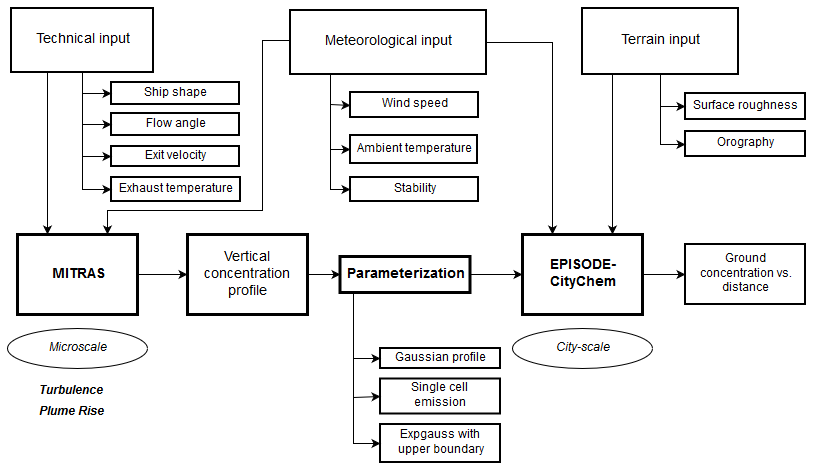
The schematic concept of this study is presented in Fig. 1. It is composed of three major parts. First, the obstacle-resolving microscale model MITRAS v2.0 (Grawe et al., 2013; Salim et al., 2018) is used to generate a set of synthetic ship plumes based on technical and meteorological input parameters. This allows studying the impact of obstacle-induced turbulence and thermal plume rise on the shape of the vertical concentration profile. The shape of these profiles is then parameterized depending on different meteorological and technical input parameters (Fig. 1; Sect. 3). In a second step, the parameterized profiles are used in the city-scale model EPISODE-CityChem v1.4 (Karl et al., 2019b; Karl and Ramacher, 2020) with various meteorological settings and additional terrain information (Sect. 4). Finally, pollution ground-level concentration values at different distances from the source are calculated and the impacts of different plume parameterizations as well as meteorological input parameters and the surface roughness are compared (Sect. 5).
To better represent microscale effects in the near field of the ship in city-scale models, it is necessary to include the effects of plume rise and turbulence into the vertical emission profile. The first step of this work is to find a good parameterization for the vertical concentration profile at a point where the plume movement is no longer affected by thermal plume rise or ship-induced turbulence, as these factors are usually not covered in larger-scale models. This is the case at a distance of around 100 m from the source (Badeke et al., 2021). At this distance, the vertical concentration profile is calculated with the microscale model MITRAS (Sect. 3.1). The resulting profiles are parameterized in three different ways, i.e., with a classical Gaussian fit (Sect. 3.2), a very simple single-cell emission assumption (Sect. 3.3) and a rather complex exponentially modified Gaussian fit with an upper plume boundary (Sect. 3.4).
3.1 MITRAS
Plume rise and turbulence effects of the source (i.e., the ship) are resolved by running a set of modeling runs with the microscale chemistry, transport and stream model (MITRAS). This non-hydrostatic, three-dimensional Eulerian model is based on the Navier–Stokes equations, the continuity equation and the conservation equations for scalar properties like temperature, humidity and concentration (Grawe et al., 2013; Salim et al., 2018; Schlünzen et al., 2003, 2018). Since the release of version 2.0, MITRAS has been extended to include radiation calculations for the human thermal environment (Fischereit, 2018); however, these extensions are not used in this study.The MITRAS configuration is the same as in Badeke et al. (2021). In short, the highest resolution is 2 m × 2 m × 2 m close to the ship in a domain of roughly 1 km × 1 km horizontally and 500 m vertically. The bottom boundary of the domain is water for which the surface roughness is calculated from the wind speed and for the presented cases is near zero. No chemical reactions occur in the simulations. A constant high temperature and a vertically directed exhaust velocity is added to the emission cell (i.e., the grid cell above the stack). More detailed information can be found in Badeke et al. (2021).
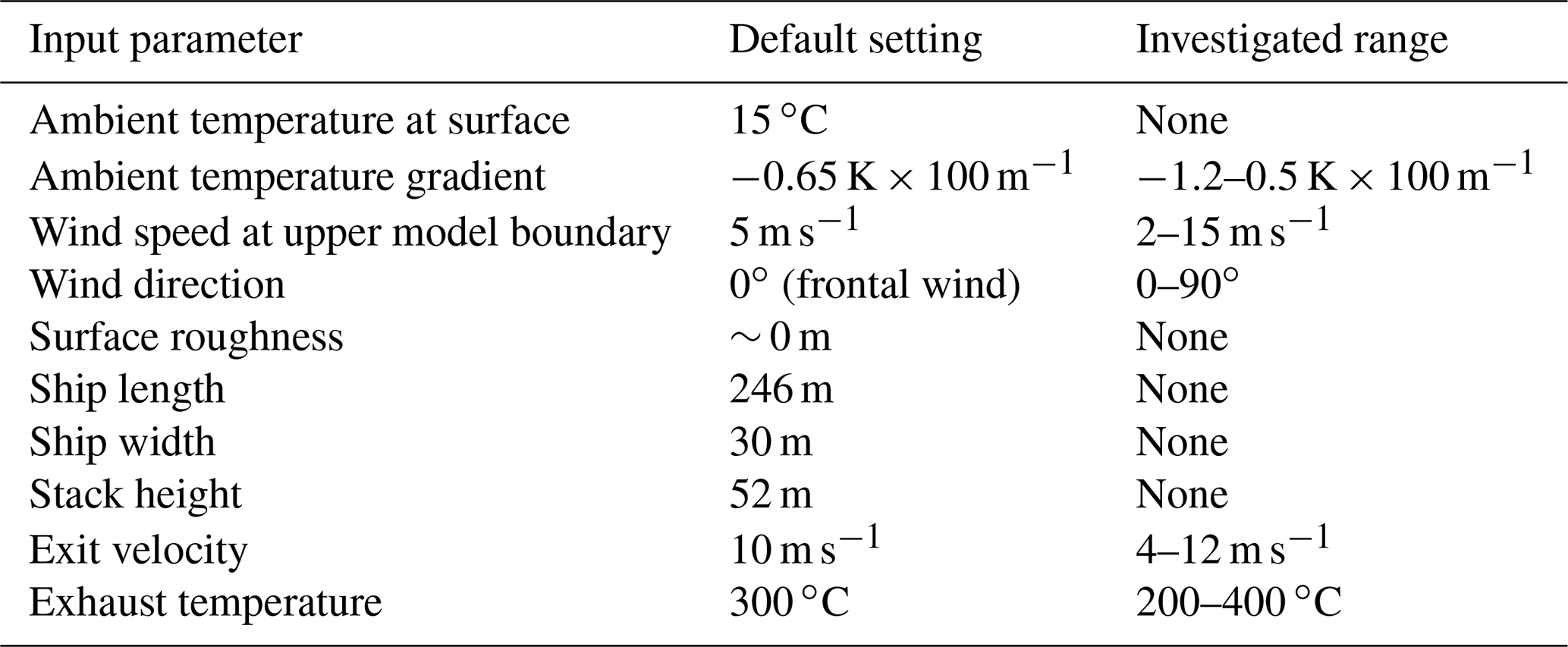
The input data for ship characteristics and meteorology are presented in Table 1. Default values are constant while for all regression analysis one input parameter at a time is varied along the investigation range. In total, 39 different cases have been calculated in MITRAS. The corresponding input values are presented in Sects. B1 and B2 in the Appendix.
Table 1Input parameters for the MITRAS calculations. While varying a single input parameter in the investigated range, all others remain at default setting (adjusted from Badeke et al., 2021).
Vertical concentration profiles are derived at a distance of 100 m away from the ship as the mean of a column with 100 m × 100 m cell sizes (see Appendix A1 for the concept). While Badeke et al. (2021) derived a formula for the downward dispersion, i.e., the fraction of concentration that is found below ship stack height, in this study, parameterizations for the whole vertical concentration profiles are calculated that account for near-field effects (thermal plume rise and obstacle-induced turbulence).
3.2 Gaussian scheme
One common way to describe the vertical dilution of a ship plume is to assume a concentration reduction according to a Gaussian curve where the mean value μ corresponds to the height of the central plume axis and the standard deviation σ describes the vertical strength of diffusion. In this way, high values of σ correspond to a plume with strong vertical diffusion that might be caused by high plume rise mainly due to high exhaust temperatures, low wind speed and/or an unstable atmosphere.
The general formula for a vertical Gaussian profile is
where c is a dimensionless concentration value and h is the height given dimensionless in [m].
A Gaussian curve was fitted to the results according to a least-square minimization with the Levenberg–Marquardt algorithm (Moré, 1977). From that, individual values for μ and σ were found.
To parameterize the Gaussian curve, the dependency of μ and σ on meteorological and technical input parameters needs to be investigated. Therefore, single regression analyses have been performed.
To estimate the effect that a single input parameter has on the value of μ or σ, all values but the one of interest for a single regression remain constant at a predefined value. These values were selected according to the previous study of Badeke et al. (2021); see Table 1.
In the single regressions in Fig. 2, the value of default setting is highlighted with a red asterisk.
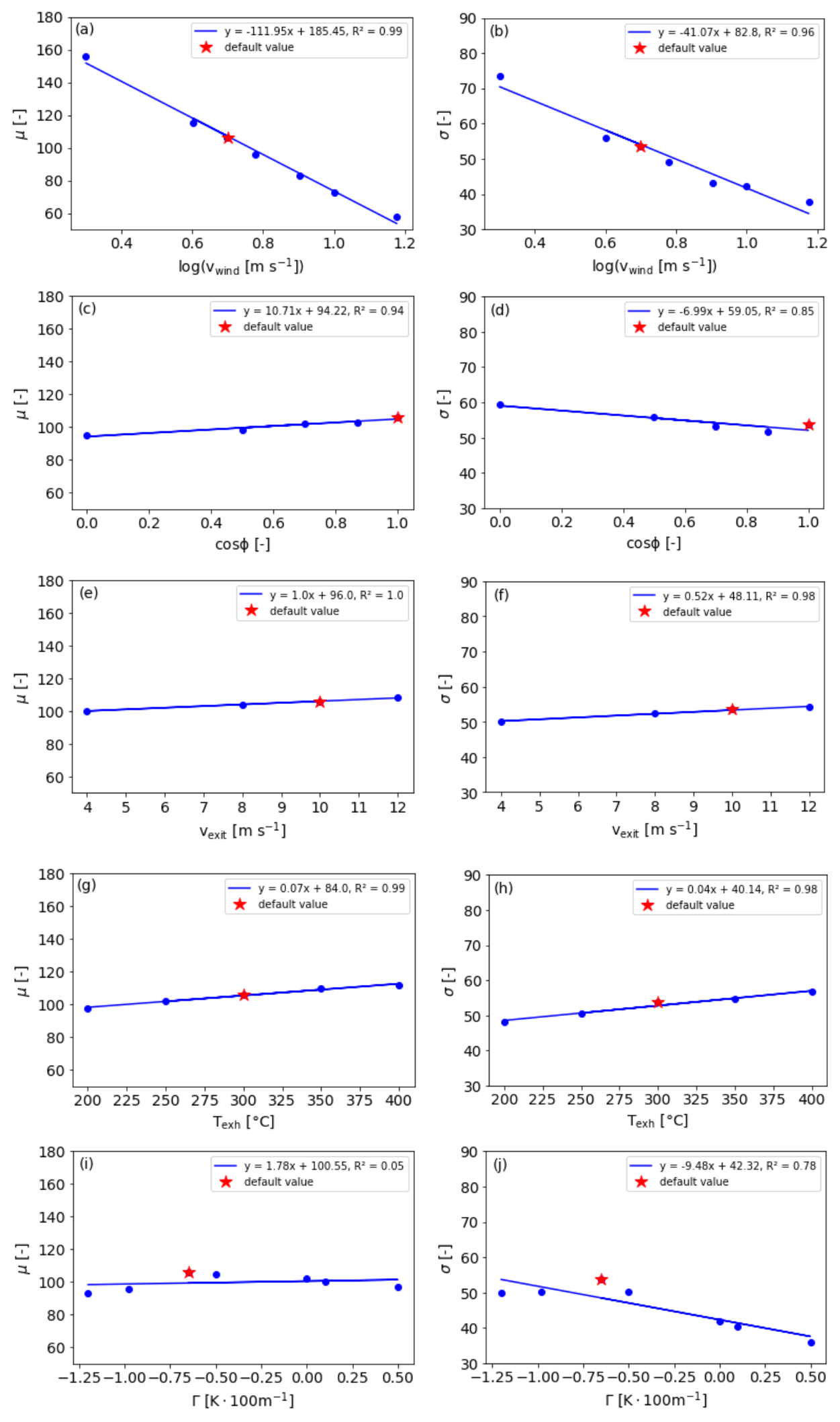
Figure 2Single regression analysis of μ and σ against the input variables wind speed (vwind), flow angle (ϕ), exit velocity (vexit), exhaust temperature (Texh) and atmospheric stability (Γ).
As visualized in the regression figures, μ and σ depend on most of the input parameters in an approximately linear way. For the wind speed, a linear correlation for μ and σ has been found against the logarithmic value of vwind, which accounts for the natural logarithmic wind profile close to the ground (Prandtl layer). The negative correlation can be interpreted as follows: higher wind speed causes the plume to remain at lower altitudes (low plume rise, low μ) and also cause a weaker vertical diffusion (lower σ). The wind speed has the strongest effect on both, μ and σ, within the investigated range of the input parameters.
A different type of linear correlation has been found for the wind angle, which describes the effect of the obstacle (i.e., the ship) orientation towards the wind direction. It ranges from 0 (frontal wind) to 90∘ (lateral wind). A positive linear dependency has been found for cos(ϕ) against μ and a negative dependency for cos(ϕ) against σ. This means that frontal wind allows for a higher plume rise (larger value of μ) but a weaker vertical dispersion (lower value of σ) than lateral wind, which can be explained by the stronger turbulent eddies that are created in the case of lateral wind (larger obstacle effect). Strong turbulence leads to a strong dispersion but at the same time weakens the plume rise.
Positive linear dependencies have been found for μ and σ against exit velocity and exhaust temperature, which both affect the initial plume rise.
No clear correlation was found for μ against the atmospheric stability (Fig. 2i). This means that, under otherwise default conditions, the atmospheric stability does not show a significant influence on the mean plume height. A negative dependency has been found for stability against σ. This means that the plume does show stronger vertical dispersion in the case of an unstable or neutral atmosphere. In a stable atmosphere (i.e., at higher values of Γ), the plume remains narrow as during very stable fanning conditions.
By applying multiple regression analysis (for more detailed insight into the procedure for ship plume studies, see Badeke et al., 2021), two functions have been determined to parameterize μ and σ based on the meteorological and technical parameters with all cases in Appendix B1.
where vwind and vexit are given dimensionless in [m s−1], Texh is given dimensionless in [K] and Γ is given dimensionless in [K × 100 m−1]
By inserting μ and σ into the Gaussian distribution equation (Eq. 1), individual Gaussian profiles can be determined and used in larger-scale Eulerian grid models for ship plumes under different meteorological and technical conditions (see Sect. 4.5).
The quality of this parameterization has been tested in two steps. In the first step, the fitting of a Gaussian curve to the original model with the Levenberg–Marquardt algorithm (Moré, 1977) has been evaluated. An average fitting quality of R2=0.92 has been found. Especially in cases of strong winds and stable atmospheric conditions, the simple Gaussian distribution delivers good results. However, in cases of strong plume rise at neutral or unstable atmospheric conditions, fitting concentration profiles with a simple Gauss can result in a poorer fitting quality of R2=0.8 (e.g., case no. 6 in Appendix B1). This reduces the applicability for Gaussian plume profiles especially in the case of air quality studies, when situations of high concentration accumulation (e.g., due to low wind speed or strong downward dispersion) have to be evaluated.
In a second step, the quality of the parameterization was tested against the fitting results, which reached an average of R2=0.99. The parameterization can reproduce the fitted curves very well.
For a complete comparison of all investigated cases, see Appendix B1 and Table C1.
3.3 Single-cell emission
A much simpler assumption is that all emission occurs in one emission height. This may be the stack height itself or an effective emission height, the latter being the case in many simple Gaussian dispersion models that solve plume rise and downward dispersion analytically.
In Eulerian grid models, the emission height equals the stack height only when the model can account for plume rise due to hot sources and turbulence due to obstacles, e.g., when using the MITRAS model.
The single-cell emission (SCE) assumption used in this model assumes all emission to enter the larger model domain (EPISODE-CityChem) at the height μ that was calculated by the Gaussian parameterization (Sect. 3.2) from MITRAS results. In this way, it accounts for plume rise and downward dispersion in a minimalistic way, since the position of the central plume axis is represented but not the initial dispersion in the first 100–200 m.
3.4 Exponentially modified Gaussian scheme with upper plume boundary
The exponentially modified Gaussian distribution (Expgauss) adds an exponential feature to the upper end on the Gaussian distribution, thereby allowing the curve to be asymmetrical. The concentration function applied here is
where c is a dimensionless concentration value and h is the height given dimensionless in [m].
It contains three shape parameters (λ1, λ2 and λ3), as well as the complementary error function erfc(x):
This density function is derived by a convolution of the normal and the exponential probability density functions. Figure 3 gives an impression on how the different shape parameters affect the curve.
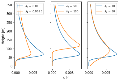
Figure 3Visualization of the effect of different shape parameters on the exponentially modified Gaussian distribution. Blue profiles are the same with λ1=0.01, λ2=50 and λ3=10, while in the orange profiles one shape parameter is varied in each panel. The concentration profile is dimensionless and needs to be normalized to serve as an initial emission input profile in EPISODE-Citychem.
λ1 is the exponential decay parameter. At λ1=1 the function resembles an ideal Gauss curve with λ2+1 as mean and λ3 as standard deviation. λ1=0 results in a constant line. λ2 affects the height of the maximum concentration and moves the curve along the y axis. It resembles the mean value of an ideal Gaussian curve when λ1=1. λ3 determines how steep the non-exponentially modified part (i.e., heights below the maximum concentration) rises. It also slightly affects the position of the concentration maximum.
As in the case of the Gaussian fit, the Expgauss curve was fitted to the results of the MITRAS simulations according to a least-square minimization with the Levenberg–Marquardt algorithm (Moré, 1977). From that, individual values for λ1, λ2 and λ3 were determined. Next, the meteorological and technical input parameters were plotted against the individual shape parameters to determine which input affects which shape parameter. Figure 4 shows the corresponding single regressions for the ranges presented in Table 1.
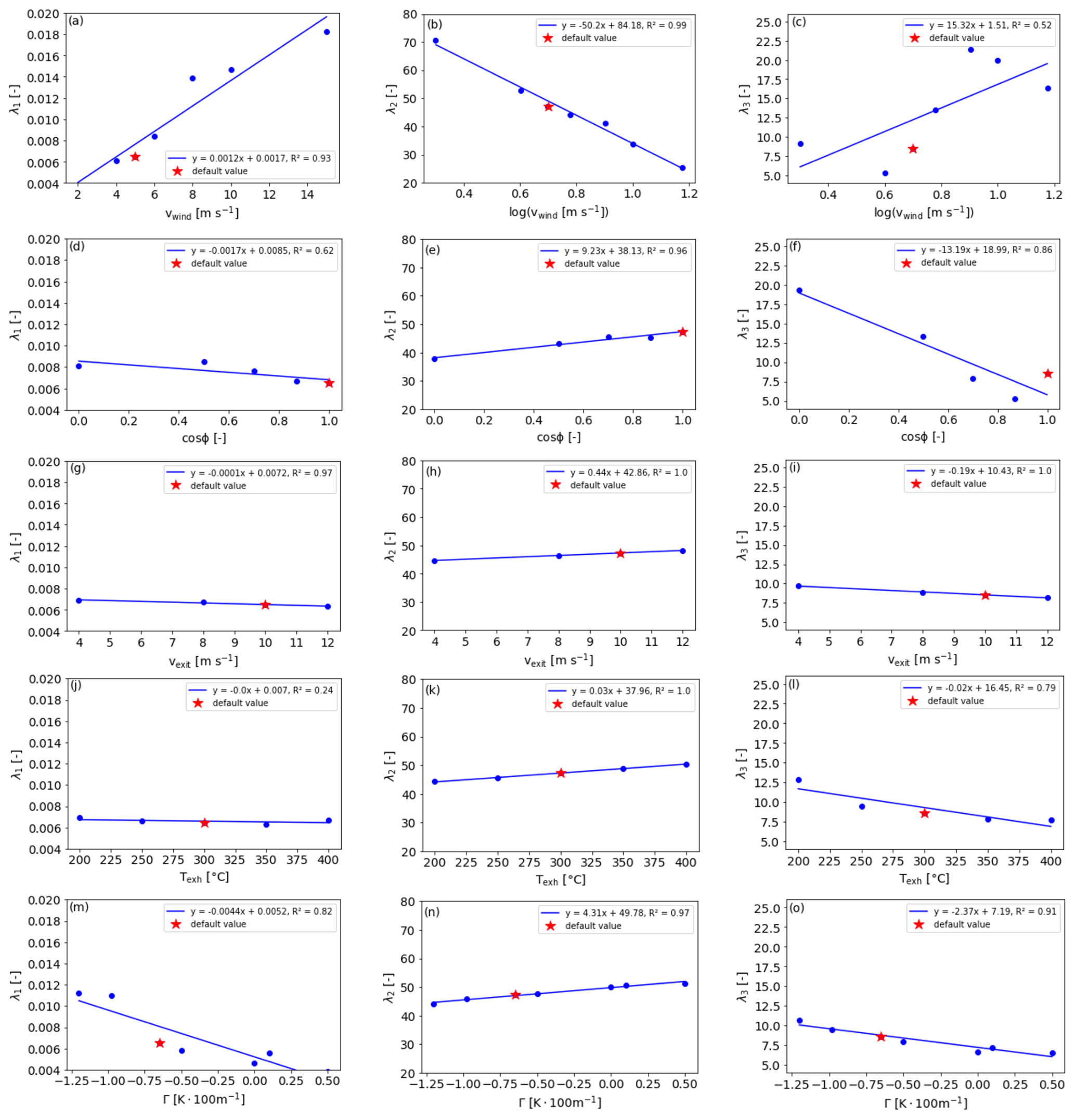
Figure 4Single regression analysis of λ1, λ2 and λ3 against the input variables wind speed (vwind), flow angle (ϕ), exit velocity (vexit), exhaust temperature (Texh) and atmospheric stability (Γ).
By applying multiple regression analysis based on the results of the strongest single regressions (see Appendix C1 for a comparison of effective ranges), the following parameterizations were found for the shape parameters:
where vwind and vexit are given dimensionless in [m s−1], Texh is given dimensionless in [K], and Γ is given dimensionless in [K × 100 m−1].
These parameterizations can then be used in Eq. (4) to calculate the vertical plume profile.
Particularly in cases of a stable atmosphere, the plume rise in the near field tends to be overestimated when fitting with an exponentially modified Gaussian function. MITRAS results show a rather sharp reduction in vertical concentration as soon as the plume temperature decreases down to ambient temperature. The height at which the plume temperature equals the ambient temperature is herein defined as upper plume boundary height hup. It was calculated based on the MITRAS model results and parameterized similar to the concentration profile functions. It can cause sharp concentration gradients in cases of a stable surrounding atmosphere.
A strong logarithmic dependency of the upper plume boundary on wind speed was found (see Fig. 5a). Larger wind speeds lead to lower maximum elevations that the plume could reach in the near field. A linear dependency was found for the upper plume boundary against exhaust temperature (Fig. 5b) and against the function sgn(Γ)Γ2 (Fig. 5c), which is the square of the vertical temperature gradient (i.e., stability) where the sign is retained (sign function). See also Badeke et al. (2021, Sect. 3.1.4) for comparable correlations for the stability.

Figure 5Regression analysis for upper plume boundary heights calculated with MITRAS against (a) wind speed (vwind), (b) exhaust temperature (Texh) and (c) atmospheric stability (Γ). Panel (d) shows the regression of the upper plume boundary from MITRAS results against the parameterization.
From these regressions, a multiple regression formula was calculated to parameterize the upper plume boundary:
where vwind is given dimensionless in [m s−1], Texh is given dimensionless in [K], and Γ is given dimensionless in [K × 100 m−1]. hup results in [m].
This parameterization was tested against MITRAS model results for a variety of 39 different scenarios (see Sects. B1 and B2 in the Appendix). A correlation of R2=0.85 for upper boundary calculation with MITRAS and the parameterization formula was found (Fig. 5d). The performance is weakest under scenarios of very low plume rise, mainly at high wind speeds (>10 m s−1). Under these conditions, one can either ignore the upper boundary condition or use the classical Gaussian profile.
Finally, the quality of the Expgauss parameterization from ground to upper plume boundary has been tested in two steps. The fitting of the Expgauss curve to the original MITRAS results delivered a mean fitting quality of R2=0.99 for all 39 investigated cases, which is better than the Gaussian fit. Furthermore, the quality of the parameterization was tested against the fitting results, which reached an average of R2=0.96. The parameterization can reproduce the fitted curves very well and only shows weaker results at high wind speeds.
For a complete comparison of all investigated cases, see Appendix C1.
Results from the Expgauss parameterization were included into further EPISODE-CityChem calculations from the ground up to the parameterized upper boundary (Sect. 4.5).
The resulting parameterization for the vertical concentration profile is integrated in the city-scale model system EPISODE-CityChem (Hamer et al., 2020; Karl et al., 2019b). This three-dimensional Eulerian grid model is used to simulate the emission, transport, dispersion, photochemical transformation and deposition of pollutants on a city-scale. In this study, the focus lies on investigating the dilution of ship plumes under varying initial emission profiles. Chemical reactions are deactivated in this study, to make it applicable to any passive tracer gas. Also, the highly nonlinear NOx–O3 chemistry would need an inclusion of background chemistry, diurnal differences for photochemistry and other sources to model NOx concentrations precisely. This was beyond the scope of this study. Therefore, gases are modeled as passive tracers.
4.1 Model setup
This section describes the specific setup and inputs selected for this study. A summary is given in Table 2.

The inner part of the city of Hamburg is simulated, representing a northern European harbor city. A horizontal resolution of 100 m × 100 m is used. The overall horizontal domain size is 8 km × 8 km.
The model uses a terrain-following sigma coordinate system defined from an idealized hydrostatic pressure distribution. A total of 30 vertical layers are used with increasing vertical expansion. In the lowest 200 m, the vertical resolution is fixed at 10 m. Above this height, it increases up to a vertical resolution of 250 m. A total height of approximately 1 km is covered. Due to the terrain-following coordinate system used, this upper limit may vary slightly.
The topography input consists of a two-dimensional static field of terrain heights that was created using the terrain pre-processor AERMAP (EPA-454/B-03-003) of the US EPA air dispersion model AERMOD (US-EPA, 2004). It coordinates the allocation of terrain elevation data from several digitized databases to a user-specified model grid. From the database of NASA's Shuttle Radar Topography Mission (SRTM, Rodriguez et al., 2006), digital elevation data have been used. They have a spatial resolution of approximately 100 m and WGS84 as reference geoid. Digital elevation data of SRTM3 for the region of Hamburg have been used with Universal Transverse Mercator (UTM) coordinates of southwest corner of the model domain being x=559 064 and y=5 930 727 (UTM zone 32N), which corresponds to 9.89091∘ E and 53.52215∘ N, respectively, in Cartesian coordinates. Topography information is converted into land-use classes and surface roughness values distinguishing only two different land-use classes: water and land. Figure 6 shows the investigation area with elevation information and an example plume.
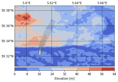
Figure 6Elevation map of the inner city of Hamburg in the EPISODE-CityChem model domain of 8 km × 8 km. An example ship plume is shown in greyscale.
The surface roughness is the height above the displacement plane at which the mean wind becomes zero when extrapolating the logarithmic wind speed profile downward through the surface layer. For water surfaces, Badeke et al. (2021) used a value close to 0 m depending on the wind speed (Schlünzen et al., 2018). Here, a fixed value of 0.001 m is used, which is reasonable, as the focus lies in the investigation of the behavior of the plume over land. The surface roughness of the land area is varied between 0.1 and 1.0 m, corresponding to different structures, from low crops to medium-sized building areas (e.g., Wieringa, 1992). It plays a major role in the computation of the friction velocity, the turbulent mixing in the vertical diffusion scheme and the dry deposition.
The meteorological field is created by the meteorological pre-processor MCWIND v1.2 (Hamer et al., 2020). This software produces a diagnostic wind field based on observational or, as in this study, synthetic data. MCWIND adjusts a first-guess wind field to a given topography in such a way that it becomes non-divergent and mass consistent. The 3-D fields are calculated internally by applying surface similarity profiles according to Monin–Obukhov theory.
Horizontal advection is considered using a positive fourth-degree Bott scheme (Bott, 1989, 1992, 1993), which calculates flux between grid cells, describing the concentration fluctuations locally. A time-splitting method is employed to solve advection separately in x and y directions.
Vertical advection is solved with an upstream scheme (Byun et al., 1999), which implicitly assumes that the 3-D wind field is free of divergence. Vertical motion is therefore either convergence or divergence in the input horizontal wind fields. This allows mass conservation.
Both horizontal and vertical eddy diffusivities are calculated on the Eulerian grid using parameterizations. The horizontal diffusion is calculated using a fully explicit forward Euler scheme (Smith, 1985). The vertical diffusion is solved according to the mixing length theory (Monin–Obukhov similarity theory) by a semi-implicit Crank–Nicolson scheme. Eddy diffusion coefficients are calculated by the urban K(z) method, presented in Hamer et al. (2020). It strongly depends on the surface roughness, which is one parameter that will be varied in this study.
The transport of pollutants in and out of the model domain is implicitly considered within the 3-D advection equations.
The effect of dry deposition is included, whereas the effect of wet deposition is not. The dry deposition is calculated based on the resistance analogy (Simpson et al., 2003).
The EPISODE-CityChem chemistry options on the Eulerian grid include a dispersion without photochemistry (applied here), a solution for basic NOx–O3 photochemical equilibrium, a detailed two-step urban chemistry solver with 45 gas-phase species (EmChem03-mod) as well as an urban chemistry scheme including heterogeneous gas-phase reactions EmChem09-HET (Simpson et al., 2012; Karl et al., 2019b).
4.2 Emission characteristics
Ship emissions are treated by EPISODE-CityChem as an area source. This means that concentrations are diluted instantaneously into the corresponding emission grid cells and emitted pollutants are then subject to advection, diffusion, deposition and chemistry (if activated) in the model grid. The vertical emission distribution corresponds to a parameterized profile derived from MITRAS results (see Appendix A1) for a column of 100 m × 100 m × 10 m downwind from the ship to account for thermal plume rise and obstacle-induced turbulence in the near field. Three different parameterization schemes are applied.
The first scheme will be standard Gaussian parameterization described in Sect. 3.2. The vertical emission profile was normalized and distributed into the corresponding cells of a vertical column.
In the single-cell assumption, the whole emission will be inserted into a single cell of the model. This will be the cell at the height of the mean value in the standard Gaussian parameterization (Sect. 3.3).
The third profile is calculated with the Expgauss parameterization (Sect. 3.4).
A normalized emission rate of 1 g s−1 NOx was selected to easier compare different effects (e.g., different concentration distribution, different meteorology or different surface roughness) on the dispersion.
A NOx split of 95 % NO and 5 % NO2 is used. However, in this study, chemical transformations are not considered, and therefore the ratio will not change, as they will behave as a passive tracer gas.
The differences of the chosen parameterization and their effect on the ground-level concentration depending on meteorological conditions and surface roughness will be evaluated. Therefore, the concentration will be calculated with increasing distance from the source along the path of highest ground-level concentration (see Appendix A2 for an exemplary scheme).
This section presents pollution ground-level concentration values at different distances from the source. The impacts of different plume parameterizations as well as meteorological input parameters and the surface roughness on the concentration values are compared and uncertainties are discussed.
5.1 Input profile
Three different methods for the initial distribution of vertical plume profiles were presented in Sect. 3. Now the differences of the resulting ground-level concentrations in dependence of the distance to the source will be examined.
As an example, Fig. 7 shows the initial emission profiles for the Gaussian and Expgauss profiles based on default input parameters, i.e., a wind speed of 5 m s−1 with frontal direction, exit velocity of 10 m s−1, exhaust temperature of 300 ∘C and an atmospheric stability of −0.65 K × 100 m−1.
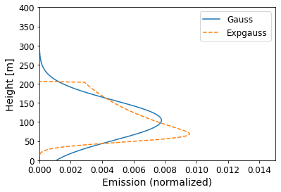
Figure 7Initial vertical emission profiles for Gaussian and exponential Gaussian emissions under default conditions (see Table 1). The single-cell emission profile lies at the mean height of the Gaussian profile with a normalized emission of 1.0 (not shown).
The concentration values in Fig. 7 are normalized, i.e., the vertically integrated emission is 1. In the case of single-cell emission, the normalized concentration value is 1 at the height of mean Gaussian distribution. For the exponential Gaussian profile the upper plume boundary of the near field lies at around 200 m. However, this upper boundary is only used for the initial emission distribution. In further EPISODE-CityChem calculations, parts of the plume might rise higher.
These normalized curves are used as initial emission profiles in EPISODE-CityChem according to the vertical resolution of the cells.
As can be seen in Fig. 7, the Gaussian profile tends to distribute a part of the emission to the lowest model layer already in the near field. Therefore, high ground-level concentration values close to the source are to be expected. The exponential Gaussian profile can better represent the plume rise. Therefore, ground-level concentrations will have a maximum at a farther distance. In the case of SCE, all emissions occur at the mean height of the Gaussian profile, i.e., with no proportion in the lowest model layer. Therefore, the peak ground-level concentration for the SCE approach occurs several 100 m downwind of the source position.
Variations of these input profiles can be found in Appendix D1 for several different initial conditions.
5.2 Effect of surface roughness
To evaluate the impact of surface roughness on pollutant ground-level concentration, the roughness value for land areas was varied between 0.1 (grassland) and 1.0 m (urban area), which was assumed to be the range of surface roughness that can occur in the harbor area. All the remaining input values were kept at default conditions (Table 1). It is important to mention that surface roughness was not included in the calculation of initial vertical plume profiles. Therefore, the initial profiles are all the same as in Fig. 7.
Figure 8 shows the ground-level concentration depending on the distance from the source, the roughness length and the effect of different initial plume profiles. For all investigated cases, the surface roughness shows larger ground-level concentration values in cases of lower surface roughness. In the case of the Gaussian profile, the highest differences occur at a distance of 700 m, where z0=0.1 m causes 2.72 µg m−3 (113 %) higher ground-level concentration than z0=1.0 m. For the SCE assumption, the maximum difference is 1.26 µg m−3 (88 %) at 1400 m distance. Finally, for the Expgauss assumption, the highest difference is 2.29 µg m−3 (128 %) at 700 m distance.
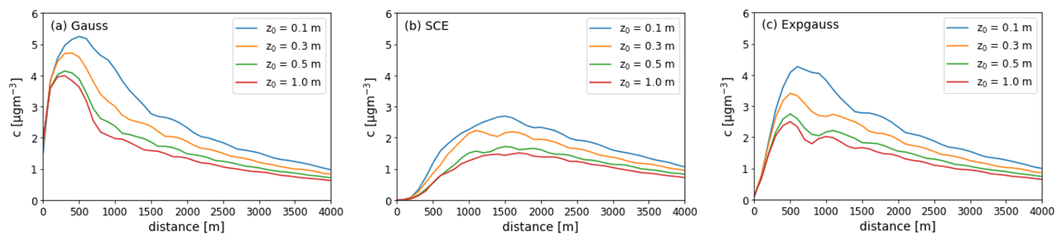
Figure 8Ground-level concentration profiles depending on the distance to the source for different roughness lengths and initial emission distribution.
Decreasing ground-level concentrations in areas of increased roughness lengths (city centers) have also been reported in a model study from Barnes et al. (2014). In their study, the lowest model layer experienced localized high ground-level concentration values of NOx in a city center where the main source of NOx is traffic. They expected a low ground-level concentration at high surface roughness due to weaker horizontal ventilation but the turbulent mixing effect dominated, thus causing lower ground-level concentrations when modeling with higher surface roughness. In our study, increased dilution also causes lower concentration values when the surface roughness is high.
When comparing the effect of initial plume profile, it can be seen that the highest ground-level concentrations occur close to the source when assuming a Gaussian distribution (see also Appendix D2). The SCE assumption shows a rather flat maximum between 1000 and 2000 m, while the Expgauss distribution shows a similar behavior as Gaussian distribution but with a smaller maximum close to the source. This can all be attributed to the ratio of emission that is initially distributed into the lower modeling layers (see Fig. 7). In the case of SCE, all emissions enter the modeling domain at a height of around 100 m and need a much longer distance to be transported downward. At a distance of around 1500 m, the ground-level concentration becomes independent of the initial plume profile.
5.3 Effects of stability
Stability effects on the ground-level concentration were tested in EPISODE-CityChem for three different temperature profiles: the standard atmosphere stability (−0.65 K × 100 m−1), a very stable atmosphere (0.0 K × 100 m−1) and an unstable atmosphere (−1.2 K × 100 m−1). Again, all the remaining input values were kept at default conditions (Table 1).
Figure 9 displays the effect of stability on the ground-level concentration for the different input concentration assumptions. For all cases, the highest ground-level concentrations are reached in the case of unstable atmospheres. This is especially strong in the nearest 1000 m. Here, the obstacle effect of the ship causes stronger turbulent mixing at high instability and more downward dispersion. Under stable conditions, the downward transport is weak and the largest proportion of the concentration remains at emission height.
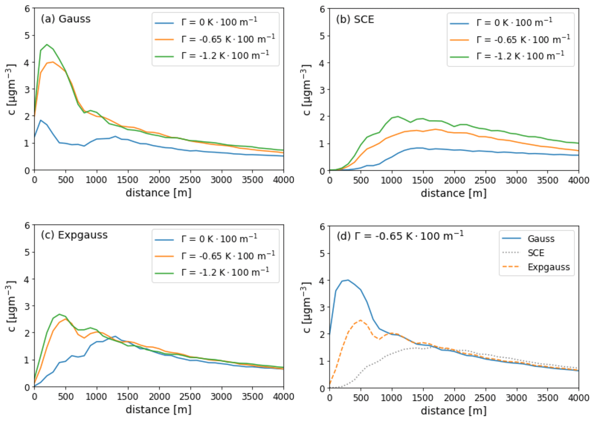
Figure 9(a–c) Ground-level concentration profiles depending on the distance to the source for different stabilities and initial emission distribution; (d) direct comparison of the effect of different emission distribution at K × 100 m−1.
For Gaussian and Expgauss profiles, the strongest absolute difference of 3.16 µg m−3 (241 %) and 2.00 µg m−3 (378 %), respectively, occurs at a distance of 200 m from the source when comparing the unstable and the very stable cases. For the SCE assumption, the highest absolute difference of 1.45 µg m−3 (302 %) occurs at a farther distance of 900 m when comparing unstable and very stable cases.
At a distance of more than 3 km, the difference in ground-level concentration between different stabilities and input profiles are almost negligible. This is caused by turbulent mixing, which is a factor of wind speed and surface roughness. Note that this distance can vary when changing the values for wind speed and surface roughness.
5.4 Effects of wind speed
EPISODE-CityChem simulations with six different wind speeds have been performed: 1, 2, 3, 5, 8 and 12 m s−1. This covers a typical range of values in northern European harbor cities (see Appendix A in Badeke et al., 2021). All the remaining input values were kept at default conditions (Table 1).
Results of ground-level concentration simulations are presented in Fig. 10. The effect of different wind speeds on the ground-level concentration is a complex phenomenon in this study. Highest concentration values are found at 1 m s−1; then there are minimum values between 3 and 5 m s−1, while at higher wind speeds, the ground-level concentration rises again.
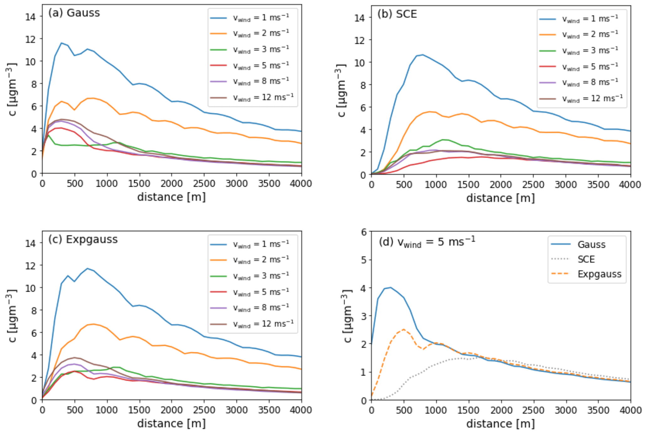
Figure 10(a–c) Ground-level concentration profiles depending on the distance to the source for different wind speeds and initial emission distribution; (d) direct comparison of the effect of different emission distribution at vwind=5 m s−1.
Two different effects cause this behavior. For slow wind speeds, advective transport is low and the pollutants accumulate to a higher rate. This alone would lead to the impression that ground-level concentrations are lowest at high wind speeds. However, a second effect increases the ground-level concentration with increasing wind speed. This is caused by the input concentration profile, which shows a weaker plume rise and a stronger obstacle-induced downward dispersion at high wind speeds (see Appendix D1 for different input profiles depending on wind speed). Badeke et al. (2021) described high wind speed as the most important factor for downward dispersion of the plume. This is caused by (a) strong turbulent eddies formed in the wake of the ship which dilutes it and (b) a weaker thermal plume rise at higher wind speeds, as the plume is transported faster and thus cools down more quickly.
Ledoux et al. (2018) also found higher concentrations with increased wind speed and described that low wind speeds rather lead to a vertical dispersion and lower concentrations.
Comparing the different parameterizations, the Gaussian profile shows the strongest differences of 9.12 µg m−3 (374 %) when comparing 1 and 3 m s−1 wind speed at a distance of 200 m. The SCE assumption shows a similar maximum absolute difference of 9.63 µg m−3 but with a much larger corresponding relative difference (1095 %) when comparing 1 and 5 m s−1 at a distance of 600 m. Finally, the Expgauss profile shows a maximum absolute difference of 9.73 µg m−3 (506 %) at 600 m when comparing 1 and 5 m s−1.
At a distance of more than 1500 m, the individual plume profiles show very similar results.
5.5 Comparison of the effects of different input variables
Table D1 summarizes the results of Sect. 5.2 to 5.4 and allows a comparison of the effect of different input variables on the ground-level concentration. Under default conditions, the strongest effect was found for wind speed variations, causing differences >9 µg m−3 or up to over 1000 %. Stability and roughness length can both cause differences in the range of 1 to 3 µg m−3 under default conditions. The strongest differences between the different input parameterizations occur in the first 1500 m from the source. Gaussian profiles give the best representation at high wind speeds and when downward dispersions near the source are strong. Expgauss profiles can better account for unstable atmospheres and strong plume rise. The SCE approach is simple but always leads to a ground-level concentration maximum at a larger distance from the source (i.e., around 1000 m downwind). This approach is certainly not optimal when measurements close to the source are underestimated.
5.6 Discussion of uncertainties
The performance of MITRAS has been verified before with quality-ensured wind tunnel data, including simple obstacle configurations and results showed a very good agreement of the wind field for most test cases (Grawe et al., 2013). The plume rise effects have been compared to the integral plume rise model IBS-PLURIS (Janicke and Janicke, 2001) in Badeke et al. (2021). The initial plume rise was generally some metres higher in the MITRAS study, as MITRAS accounts for the change in the thermodynamic field and the heat balance equation creates additional buoyancy that is not accounted for in simple Gaussian approaches.
The performance of EPISODE-CityChem has been evaluated in Karl et al. (2019b) with a series of statistical tests, including comparisons against the standard EPISODE model, the air pollution model (TAPM; Hurley et al., 2005; Hurley, 2008) and measurements in the city of Hamburg. It fulfils the model performance objectives set for the air quality directive, which qualifies it for use in policy applications. From these previous performance evaluations, it is assumed that the model setup in this study is capable of reproducing ship plume scenarios in a realistic manner.
In the EPISODE-CityChem part of this study, the ship plume is classified as an area source and not a point source as in the majority of plume model studies (e.g., Poplawski et al., 2011; Merico et al., 2019; Bai et al., 2020; Pan et al., 2021). This can lead to a poorer performance at lower grid resolutions when the emission is instantaneous diluted equally into the corresponding emission cells (e.g., Huszar et al., 2010; Vinken et al., 2011; Jonson et al., 2015). Studies that treat ship emissions as area sources are rather rare (Kotrikla et al., 2013; Abrutytė et al., 2014). However, in this study, the emission profile is adjusted based on MITRAS parameterizations of the initial plume distribution, accounting for plume rise and obstacle-induced turbulence in the near field. The MITRAS results are based on a point source approach, where emissions enter the grid in a 2 m × 2 m × 2 m grid (Badeke et al., 2021). Afterwards, the plume concentration profile is used for the vertical emission distribution in the EPISODE-CityChem model. At a distance of roughly 100 m from the source, a dilution of the plume to a 100 m × 100 m area source can be considered acceptable and the equally dilution error is further reduced when applying Gaussian or Expgauss vertical distribution.
Applying Monin–Obukhov similarity theory for the vertical wind profile in the surface layer has a limitation for models with a high vertical resolution. The logarithmic wind profile is inaccurate inside the surface roughness layer in cases where the surface roughness is not considerably smaller than the lowest model layer height and the wind speed then tends to be overestimated (e.g., Lee et al., 2020). Basu and Lacser (2017) presented an overview of this issue recommending the modeling community to follow a guideline of z1>50 z0, where z1 corresponds to the lowest model layer height. This condition is not fully satisfied in some of the EPISODE-CityChem simulations with higher surface roughness. However, EPISODE-CityChem includes empirical stability correction functions for the surface layer wind profile that address this problem (Holtslag, 1984; Holtslag and de Bruin, 1988), and from the results herein, no evidence of inaccuracies in the plume dispersion even at higher surface roughness was found.
Input assumptions are based on a medium-sized cruise ship with a stack height of approximately 50 m. The selected range of input values such as exit velocity and exhaust temperature have already been discussed by Badeke et al. (2021). For smaller ships, the distribution curves can vary. An adjustment to different stack heights is possible and in a first approximation done by shifting the emission distribution by the difference of the chimney heights. A complete validation of the vertical profiles is only possible by comparing them with real measurements that also need the inclusion of correct emission factors, other sources and chemistry effects. A precise estimation of emission factors of moored ships includes a further uncertainty, namely the inaccurate data basis for the use of auxiliary engines that are used during hoteling. Most studies investigate emissions of main engines, while only a few specifically measured or modeled auxiliary engines (e.g., Abrutytė et al., 2014; Cooper, 2003; Eyring et al., 2005; Moreno-Gutiérrez et al., 2015; Tzannatos, 2010). Large ships have generally between three and seven auxiliary engines (Jayaram et al., 2011), and uncertainties arise from individual engine operating days, engine load, the specific fuel consumption and the kind of performed operation, e.g., hoteling or loading (Cooper, 2003; Moreno-Gutiérrez et al., 2015).
The authors assume that besides the variety of uncertainties, the results of this study have a relevant practical implication in real cases, most importantly due to including the wind speed as a variable into the calculation of vertical emission profiles, which has the largest impact on the emission distribution and resulting concentrations. Since wind speed measurements are widely available, an inclusion of wind speeds into the distribution function is possible in any real case scenario. Further uncertainties like technical parameters can be extracted from engine data sheets for individual ships and, if not available, be extrapolated from similar ships or engines. An important tool to derive this information for individual ships is the recently developed ship emission modeling system MoSES (Schwarzkopf et al., 2021).
Including all of this was beyond the scope of this study but the inclusion of the new emission profiles into a more complex chemistry transport model study is planned for the future.
This study served to improve the modeling of ship exhaust gases on the city scale with regard to the vertical pollutant distribution. In a first step, vertical concentration profiles were calculated using the microscale MITRAS model, which takes into account plume rise and obstacle turbulence. This was done for various meteorological and ship-technical conditions to cover a variety of possible scenarios in northern Europe harbor cities. From the MITRAS results, three different parameterizations for the emission distribution in the city-scale model EPISODE-CityChem were derived. Their effects on the urban ground-level concentration have been compared under conditions of varying urban surface roughness, wind speed and atmospheric stability.
Based on the model results of this study, the authors would like to make recommendations for which vertical plume parameterization should be used and when. A general differentiation is recommended for studies with horizontal resolutions ≤4 km, i.e., especially on the city scale. At a larger distance from the source, the profiles deliver approximately the same results for pollution close to the ground. Therefore, a simple single-cell emission is sufficient for open-ocean or regional studies with horizontal resolutions >4 km. Note that the emissions should still be inserted into the correct vertical cell. Equation (2) is then used to calculate the emission height.
At smaller scales, authors recommend the use of a Gaussian profile in the case of moderate or strong wind speeds (>5 m s−1) and neutral to stable atmosphere (Γ>−1.0 K × 100 m−1). Regression results for the parameterization were close to R2=1.0 in these cases. A vertical Gaussian distribution for stable boundary layers has also been applied for a ship emission study with AERMOD (Cohan et al., 2011). Gaussian parameterization can also be recommended in the case of moving ship studies, e.g., Pan et al. (2021), since ship speed and wind speed often sum up to a higher effective wind speed, which should then be used in the parameterization formulae.
For calm wind situations or unstable atmospheres, which can occur in harbors under hoteling situations, the Expgauss parameterization can better account for the initial plume rise and is recommended. A comparable result is expected by applying the bi-Gaussian distribution, which is used in the case of convective boundary layers in AERMOD (e.g., Cohan et al., 2011). The Expgauss parameterization is of special interest for air quality studies, since pollutant accumulation usually occurs at low wind speeds. To the authors' knowledge, this approach is the first of its kind to develop a dynamic vertical emission profile for ship emissions, including effects of plume rise and downward dispersion and it allows an adjustment of the emission profile for each time step. This is especially useful in cases of moving sources where the ship orientation and flow angle change frequently. A future study is planned to combine results of this study with the moving point source approach from Pan et al. (2021) for the EPISODE-CityChem modeling system. This will allow a time-flexible variation of the vertical profile of shipping emissions with either the Gaussian or Expgauss profiles derived here.
Figure A1 describes the scheme after which vertical concentration profiles from MITRAS have been derived. These concentration profiles were later normalized and used as vertical emission profiles in EPISODE-CityChem.
Figure A2 describes the scheme for deriving ground-level concentration versus distance plots.
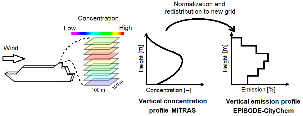
Figure A1Scheme for deriving the vertical plume concentration profile from MITRAS and transformation into emission profiles in EPISODE-CityChem. Dimensionless concentration values are derived from mean column values of 100 m × 100 m horizontal and 10 m vertical size in a distance of 100 m downwind from the ship to include plume rise and obstacle-induced turbulence. Normalization of the concentration profile and redistribution into the coarser EPISODE-CityChem grid is done to derive the vertical emission profile in EPISODE-CityChem. The figure has been adjusted and expanded from Badeke et al. (2021).
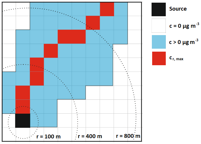
Figure A2Scheme for deriving ground-level concentration versus distance plots. Top view of the lowest model layer grid. The grid has a resolution of 100 m × 100 m. Blue cells are affected by the plume concentration; while white cells are not. For every radius of r=100 m to r=4000 m, a circular function is applied to determine the highest concentration value along the perimeter. This is exemplarily shown for r=100, 400 and 800 m. Red cells show the resulting path of highest ground-level concentration.
Tables B1 and B2 present the results of the Gaussian and Expgauss regression analyses, based on which Eqs. (2), (3) and (6)–(9) have been derived.
Table B1Data table for Gaussian regression analyses. Input data are wind speed at stack height of 50 m (vwind), exit velocity (vexit), exhaust temperature (Texh) and wind direction (ϕ), with 0∘ referring to frontal and 90∘ to lateral wind, and atmospheric stability (Γ). Results are mean (μ), standard deviation (σ) and regression coefficient (R2) for the regression analysis of MITRAS results against the fitted Gaussian functions and regression of fit against parameterization. The bold values in line no. 8 correspond to the default settings.

Table B2Data table for Expgauss regression analyses. Input data are wind speed at stack height of 50 m (vwind), exit velocity (vexit), exhaust temperature (Texh) and wind direction (ϕ), with 0∘ referring to frontal and 90∘ to lateral wind, and atmospheric stability (Γ). Results are upper plume boundary height (hup), shape parameters for the Expgauss function (λ1, λ2, λ3) and regression coefficient (R2) for the regression analysis of MITRAS results against the fitted Expgauss functions and regression of fit against parameterization. The bold values in line no. 8 correspond to the default settings.
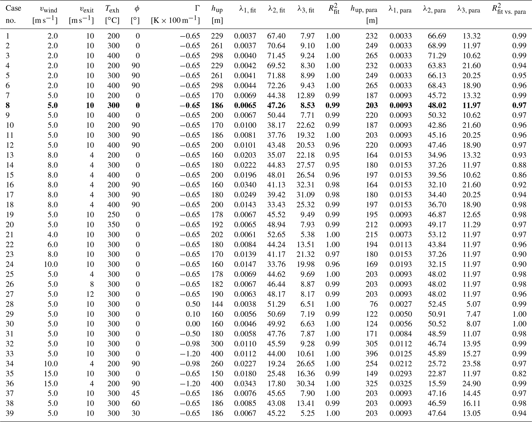
Table C1 presents a quantitative comparison of how strong the different input parameters affect the shape parameters for Gaussian and Expgauss fits.
Table C1Quantitative representation of how strong input parameters affect the shape parameters for Gaussian and Expgauss fits. Values in the table indicate the possible change that an input variable could cause on the concentration profile shape parameters (while all other inputs remained at default conditions, comparable to effective ranges in Badeke et al., 2021). Bold values were used for the parameterization as they had both a strong impact and a clear correlation.
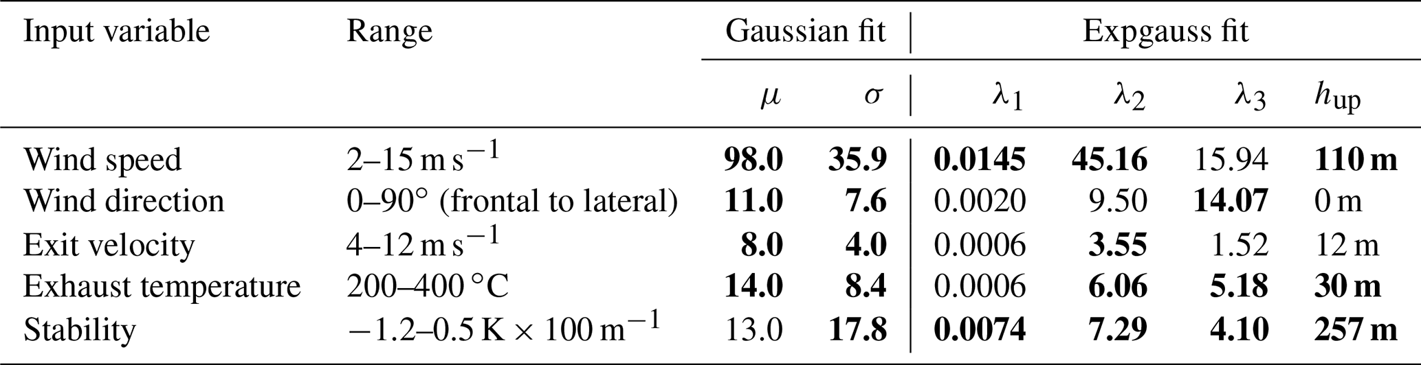
Figure D1 presents different input profiles for the EPISODE-CityChem simulation part of this study and the effect of atmospheric stability and wind speed on the profile shape. Figure D2 compares ground-level concentration values depending on the distance to the source for different settings and initial profiles. Table D1 summarizes the results of Sect. 5.2 to 5.4 and allows a comparison of the effect of different input variables on the ground-level concentration. Maximum absolute concentration differences (Δcmax) for the individual variable (surface roughness, stability, wind speed) and initial emission profile (Gauss, SCE, Expgauss) are presented.
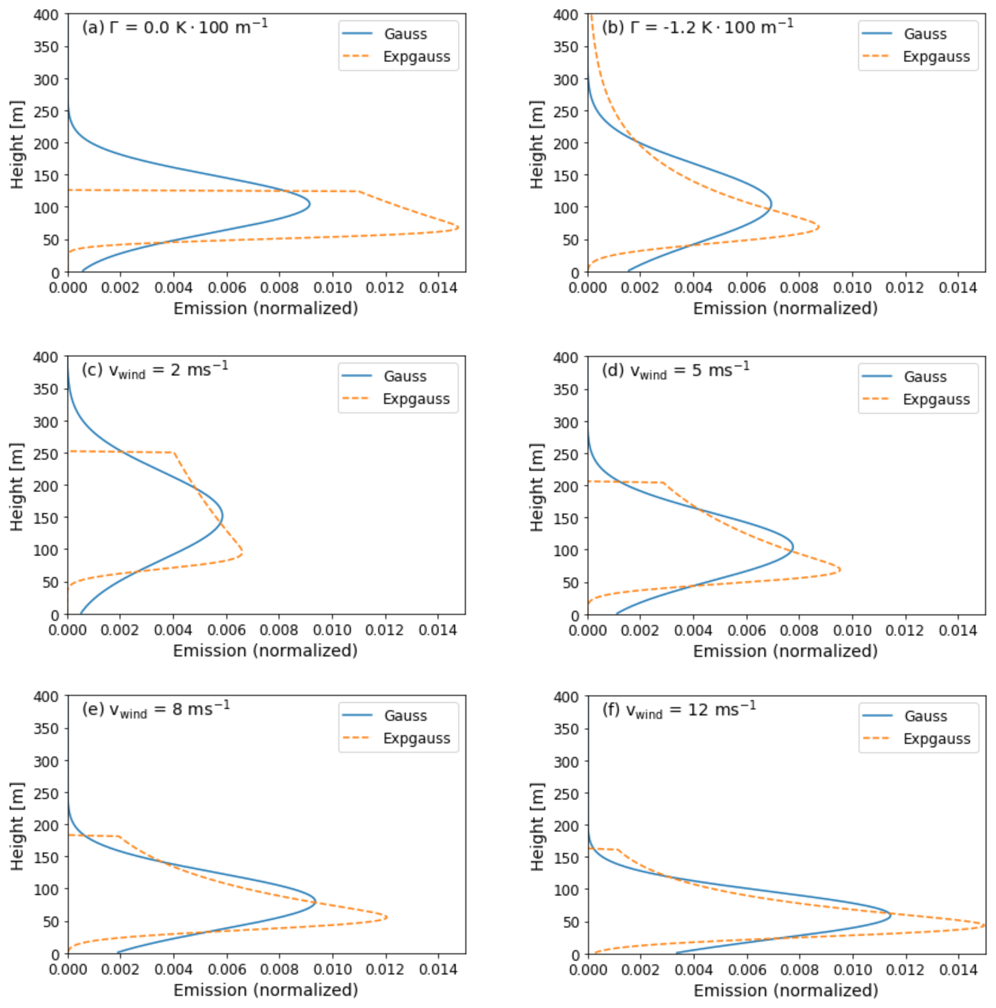
Figure D1Initial EPISODE-CityChem emission profiles under default input settings (vwind=5 m s−1, vexit=10 m s−1, Texh=300 ∘C, K × 100 m−1, ϕ=0∘ and m) for all but one parameter. Panels (a) and (b) show effects of varying the stability, while panels (c)–(f) show effects of varying the wind speed. Panel (d) represents full default conditions.
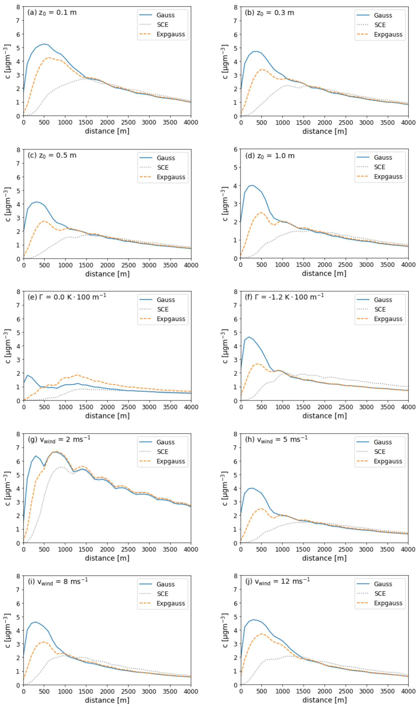
Figure D2Comparison for ground-level concentration values depending on the distance to the source for different settings and initial profiles. Default input settings (vwind=5 m s−1, vexit=10 m s−1, Texh=300 ∘C, K × 100 m−1, ϕ=0∘ and m) were used for all but one parameter. Panels (a)–(d) vary roughness lengths over land; panels (e) and (f) vary atmospheric stability. Panels (g)–(j) vary wind speed. Panel (h) represents full default conditions.
Table D1Comparison of effects of different input variables and initial emission profiles on the ground-level concentration. Values of Δcmax correspond to the highest absolute differences. Their corresponding relative difference is added in parentheses and the distance of Δcmax is given as well.

Currently, the MITRAS source code is distributed upon request under the terms of a user agreement with the Mesoscale and Microscale Modeling (MeMi) working group at the Meteorological Institute, University of Hamburg (https://www.mi.uni-hamburg.de/memi, University of Hamburg, 2022). A copy of the user agreement is available upon request. Due to current copyright restrictions, users are requested to contact the corresponding authors to obtain access to the code free of charge for research purposes under a collaboration agreement (metras@uni-hamburg.de). Documentation for the M-SYS model system in which MITRAS is included is available online at https://www.mi.uni-hamburg.de/memi under “Numerical Models”.
The source codes of the EPISODE-CityChem model version 1.4 and the pre-processing utilities are accessible in release under the RPL license at https://doi.org/10.5281/zenodo.3862264 (Karl and Ramacher, 2020). Pre-processing tools for EPISODE-CityChem are written in Fortran 90. Software requirements for the utilities and the EPISODE-CityChem model are installation of the gcc/gfortran Fortran 90 compiler (version 4.4 or later) and the NetCDF library (version 3.6.0 or later).
Regression data and a Python scripts for calculating the different vertical plume profiles as well as hup have been added in the Supplement and uploaded at https://doi.org/10.5281/zenodo.5675747 (Badeke, 2021).
The supplement related to this article is available online at: https://doi.org/10.5194/gmd-15-4077-2022-supplement.
All authors were responsible for the conceptualization; RB and DG formulated the methodology and plume parameterization; RB and MK formulated the EPISODE-CityChem chapter; all authors contributed to the discussion and conclusion; RB was responsible for the writing. All authors have read and agreed to the published version of the manuscript.
The contact author has declared that neither they nor their co-authors have any competing interests.
Publisher’s note: Copernicus Publications remains neutral with regard to jurisdictional claims in published maps and institutional affiliations.
The authors would kindly like to thank Bernd Leitl and Kay-Christian Emeis for the fruitful discussions during the preparation of the manuscript.
This research has been supported by the Deutsche Forschungsgemeinschaft (grant no. 645514).
The article processing charges for this open-access publication were covered by the Helmholtz-Zentrum Hereon.
This paper was edited by Christoph Knote and reviewed by two anonymous referees.
Abrutytė, E., Žukauskaitė, A., Mickevičienė, R., Zabukas, V., and Paulauskienė, T.: Evaluation of NOx emission and dispersion from marine ships in Klaipeda Sea port, J. Environ. Eng. Landsc., 22, 264–273, https://doi.org/10.3846/16486897.2014.892009, 2014.
Aksoyoglu, S., Baltensperger, U., and Prévôt, A. S. H.: Contribution of ship emissions to the concentration and deposition of air pollutants in Europe, Atmos. Chem. Phys., 16, 1895–1906, https://doi.org/10.5194/acp-16-1895-2016, 2016.
Anderson, J. O., Thundiyil, J. G., and Stolbach, A.: Clearing the air: A review of the effects of particulate matter air pollution on human health, J. Med. Toxicol., 8, 166–175, https://doi.org/10.1007/s13181-011-0203-1, 2012.
Andersson, C., Bergström, R., and Johansson, C.: Population exposure and mortality due to regional background PM in Europe – Long-term simulations of source region and shipping contributions, Atmos. Environ., 43, 22–23, https://doi.org/10.1016/j.atmosenv.2009.03.040, 2009.
Badeke, R.: Vertical ship emission profile parameterization, Zenodo [data set], https://doi.org/10.5281/zenodo.5675747, 2021.
Badeke, R., Matthias, V., and Grawe, D.: Parameterizing the vertical downward dispersion of ship exhaust gas in the near field, Atmos. Chem. Phys., 21, 5935–5951, https://doi.org/10.5194/acp-21-5935-2021, 2021.
Bai, S., Wen, Y., He, L., Liu, Y., Zhang, Y., Yu, Q., and Ma, W.: Single-vessel plume dispersion simulation: Method and a case study using CALPUFF in the Yantian port area, Shenzhen (China), Int. J. Env. Res. Pub. He., 17, 7821, https://doi.org/10.3390/ijerph17217831, 2020.
Barnes, M. J., Brade, T. K., MacKenzie, A. R., Whyatt, J. D., Carruthers, D. J., Stocker, J., Cai, X., and Hewitt, C. N.: Spatially-varying surface roughness and ground-level air quality in an operational dispersion model, Environ. Pollut., 185, 44–51, https://doi.org/10.1016/j.envpol.2013.09.039, 2014.
Basu, S. and Lacser, A.: A cautionary note on the use of Monin-Obukhov similarity theory in very high-resolution Large-Eddy-Simulations, Bound.-Lay. Meteorol., 163, 351–355, https://doi.org/10.1007/s10546-016-0225-y, 2017.
Bieser, J., Aulinger, A., Matthias, V., Quante, M., and van der Gon, H. A. C. D.: Vertical emission profiles for Europe based on plume rise calculations, Environ. Pollut., 159, 2935–2946, https://doi.org/10.1016/j.envpol.2011.04.030, 2011.
Bott, A.: A positive definite advection scheme obtained by nonlinear renormalization of the advective fluxes, Mon. Weather Rev., 117, 1006–1016, 1989.
Bott, A.: Monotone flux limitation in the area-preserving flux-form advection algorithm, Mon. Weather Rev., 120, 2592–2602, 1992.
Bott, A.: The monotone area-preserving flux-form advection algorithm: Reducing the time-splitting error in two-dimensional flow fields, Mon. Weather Rev., 121, 2638–2641, 1993.
Brandt, J., Silver, J. D., Christensen, J. H., Andersen, M. S., Bønløkke, J. H., Sigsgaard, T., Geels, C., Gross, A., Hansen, A. B., Hansen, K. M., Hedegaard, G. B., Kaas, E., and Frohn, L. M.: Assessment of past, present and future health-cost externalities of air pollution in Europe and the contribution from international ship traffic using the EVA model system, Atmos. Chem. Phys., 13, 7747–7764, https://doi.org/10.5194/acp-13-7747-2013, 2013.
Briggs, G. A.: Plume rise predictions, in: Lectures on air pollution and environmental impact analyses, American Meteorological Society, Boston, MA, https://doi.org/10.1007/978-1-935704-23-2_3, 1982.
Broome, R. A., Cope, M. E., Goldsworthy, B., Goldsworthy, L., Emmerson, K., Jegasothy, E., and Morgan, G. G.: The mortality effect of ship-related fine particulate matter in the Sydney greater metropolitan region of NSW, Australia, Environ. Int., 87, 85–93, https://doi.org/10.1016/j.envint.2015.11.012, 2016.
Brunner, D., Kuhlmann, G., Marshall, J., Clément, V., Fuhrer, O., Broquet, G., Löscher, A., and Meijer, Y.: Accounting for the vertical distribution of emissions in atmospheric CO2 simulations, Atmos. Chem. Phys., 19, 4541–4559, https://doi.org/10.5194/acp-19-4541-2019, 2019.
Byun, D. W., Young, J., Pleim, J., Odman, M. T., and Alapaty, K.: Numerical transport algorithms for the Community Multiscale Air Quality (CMAQ) chemical transport model in generalized coordinates, in: Science Algorithms of the EPA Models-3 Community Multiscale Air Quality (CMAQ) Modeling System, edited by: Byun, D. W. and Ching, J. K. S., National Exposure Research Laboratory, U.S. EPA, Research Triangle Park, NC, Chap. 7, EPA/600/R-99/030, https://nepis.epa.gov/Exe/ZyPDF.cgi?Dockey=30003R9Y.PDF (last access: 24 May 2022), 1999.
Chosson, F., Paoli, R., and Cuenot, B.: Ship plume dispersion rates in convective boundary layers for chemistry models, Atmos. Chem. Phys., 8, 4841–4853, https://doi.org/10.5194/acp-8-4841-2008, 2008.
Cohan, A., Wu, J., and Dabdub, D.: High-resolution pollutant transport in the San Pedro Bay of California, Atmos. Pollut. Res., 2, 237–246, https://doi.org/10.5094/APR.2011.030, 2011.
Contini, D. and Merico, E: Recent advances in studying air quality and health effects of shipping emissions, Atmosphere, 12, 92, https://doi.org/10.3390/atmos12010092, 2021.
Cooper, D. A.: Exhaust emissions from ships at berth, Atmos. Environ., 37, 3817–3830, https://doi.org/10.1016/S1352-2310(03)00446-1 , 2003.
Corbett, J. J., Winebrake, J. J., Green, E. H., Kasibhatla, P., Eyring, V., and Lauer, A.: Mortality from ship emissions: A global assessment, Environ. Sci. Technol., 41, 8512–8518, https://doi.org/10.1021/es071686z, 2007.
European Union: Directive 2008/50/EC of the European Parliament and of the Council of 21 May 2008 on ambient air quality and cleaner air for Europe. O . J. Eur. Union, 51, 1–44, https://eur-lex.europa.eu/legal-content/EN/TXT/PDF/?uri=OJ:L:2008:152:FULL&from=EN (last access: 24 May 2022), 2008.
Eyring, V., Köhler, H. W., van Aardenne, J., and Lauer, A.: Emissions from international shipping: 1. The last 50 years, J. Geophys. Res., 110, D17305, https://doi.org/10.1029/2004JD005619, 2005.
Eyring, V., Isaksen, I. S. A., Berntsen, T., Collins, W. J., Corbett, J. J., Endresen, O., Grainger, R. G., Moldanova, J., Schlager, H., and Stevenson, D. S.: Transport impacts on atmosphere and climate: Shipping, Atmos. Environ., 44, 4735–4771, https://doi.org/10.1016/j.atmosenv.2009.04.059, 2010.
Fischereit, J.: Influence of urban water surfaces on human thermal environments – an obstacle resolving modelling approach, PhD thesis, University Hamburg, Germany, 383 pp., https://ediss.sub.uni-hamburg.de/handle/ediss/8005 (last access: 24 May 2022), 2018.
Fridell, E., Steen, E., and Peterson, K.: Primary particles in ship emissions, Atmos. Environ., 42, 1160–1168, https://doi.org/10.1016/j.atmosenv.2007.10.042, 2008.
Grawe, D., Schlünzen, K. H., and Pascheke, F.: Comparison of results of an obstacle resolving microscale model with wind tunnel data, Atmos. Environ., 79, 495–509, https://doi.org/10.1016/j.atmosenv.2013.06.039, 2013.
Hamer, P. D., Walker, S.-E., Sousa-Santos, G., Vogt, M., Vo-Thanh, D., Lopez-Aparicio, S., Schneider, P., Ramacher, M. O. P., and Karl, M.: The urban dispersion model EPISODE v10.0 – Part 1: An Eulerian and sub-grid-scale air quality model and its application in Nordic winter conditions, Geosci. Model Dev., 13, 4323–4353, https://doi.org/10.5194/gmd-13-4323-2020, 2020.
Hanna, S. R., Schulman, L. L., Paine, R. J., Pleim, J. E., and Baer, M.: Development and evaluation of the offshore and coastal dispersion model, J. Air Pollut. Control Assoc., 35, 1039–1047, https://doi.org/10.1080/00022470.1985.10466003, 1985.
Hanna, S. R., Egan, B. A., Purdum, J., and Wagler, J.: Evaluation of the ADMS, AERMOD and ISC3 dispersion models with the OPTEX, Duke Forest, Kincaid, Indianapolis and Lovett field datasets, Int. J. Environ. Pollut., 16, 301–314, https://doi.org/10.1504/IJEP.2001.000626, 2001.
Holtslag A. A. M.: Estimates of diabatic wind speed profiles from near-surface weather observations, Bound.-Lay. Meteorol., 29, 225–250, 1984.
Holtslag, A. A. M. and de Bruin, H. A. R.: Applied modeling of the nighttime surface energy balance over land, J. Appl. Meteorol., 27, 689–704, 1988.
Hulskotte, J. H. J. and Denier van der Gon, H. A. C.: Fuel consumption and associated emissions from seagoing ships at berth derived from an on-board survey, Atmos. Environ., 44, 1229–1236, https://doi.org/10.1016/j.atmosenv.2009.10.018, 2010.
Hunter, K. A., Liss, P. A., Surapipith, V., Dentener, F., Duce, R., Kanakidou, M., Kubilay, N., Mahowald, N., Okin, G., Sarin, M., Uematsu, M., and Zhu, T.: Impacts of anthropogenic SOx, NOx and NH3 on acidification of coastal waters and shipping lanes, Geophys. Res. Lett., 38, L13602, https://doi.org/10.1029/2011GL047720, 2011.
Hurley P.: TAPM v. 4, Part 1: Technical Description, CSIRO Marine and Atmospheric Research Paper No. 25, Aspendale, Vic., Australia, ISBN 978-1-921424-71-7, https://www.cmar.csiro.au/research/tapm/docs/tapm_v4_technical_paper_part1.pdf (last access: 24 May 2022), 2008.
Hurley, P., Physick, W., and Luhar, A.: TAPM – a practical approach to prognostic meteorological and air pollution modelling, Environ. Modell. Softw., 20, 737–752, https://doi.org/10.1016/j.envsoft.2004.04.006, 2005.
Huszar, P., Cariolle, D., Paoli, R., Halenka, T., Belda, M., Schlager, H., Miksovsky, J., and Pisoft, P.: Modeling the regional impact of ship emissions on NOx and ozone levels over the Eastern Atlantic and Western Europe using ship plume parameterization, Atmos. Chem. Phys., 10, 6645–6660, https://doi.org/10.5194/acp-10-6645-2010, 2010.
Jahangiri, S., Nikolova, N., and Tenekedjiev, K.: Application of a developed dispersion model to port of Brisbane, American J. Environ. Sci., 14, 156–169, https://doi.org/10.3844/ajessp.2018.156.169, 2018.
Jalkanen, J.-P., Brink, A., Kalli, J., Pettersson, H., Kukkonen, J., and Stipa, T.: A modelling system for the exhaust emissions of marine traffic and its application in the Baltic Sea area, Atmos. Chem. Phys., 9, 9209–9223, https://doi.org/10.5194/acp-9-9209-2009, 2009.
Jalkanen, J.-P., Johansson, L., Kukkonen, J., Brink, A., Kalli, J., and Stipa, T.: Extension of an assessment model of ship traffic exhaust emissions for particulate matter and carbon monoxide, Atmos. Chem. Phys., 12, 2641–2659, https://doi.org/10.5194/acp-12-2641-2012, 2012.
Janicke, U. and Janicke, L.: A three-dimensional plume rise model for dry and wet plumes, Atmos. Environ., 35, 877–890, https://doi.org/10.1016/S1352-2310(00)00372-1, 2001.
Jayaram, V., Nigam, A., Welch, W. A., Miller, J. W., and Cocker III, D. R.: Effectiveness of emission control technologies for auxiliary engines on ocean-going vessels, J. Air. Waste Manage., 61, 14–21, https://doi.org/10.3155/1047-3289.61.1.14, 2011.
Johansson, L., Jalkanen, J. P., and Kukkonen, J.: Global assessment of shipping emissions in 2015 on a high spatial and temporal resolution, Atmos. Environ., 167, 403–415, https://doi.org/10.1016/j.atmosenv.2017.08.042, 2017.
Jonson, J. E., Jalkanen, J. P., Johansson, L., Gauss, M., and Denier van der Gon, H. A. C.: Model calculations of the effects of present and future emissions of air pollutants from shipping in the Baltic Sea and the North Sea, Atmos. Chem. Phys., 15, 783–798, https://doi.org/10.5194/acp-15-783-2015, 2015.
Karl, M. and Ramacher, M.: City-scale Chemistry Transport Model EPISODE-CityChem (Release version 1.4), Zenodo [code], https://doi.org/10.5281/zenodo.3862264, 2020.
Karl, M., Bieser, J., Geyer, B., Matthias, V., Jalkanen, J.-P., Johansson, L., and Fridell, E.: Impact of a nitrogen emission control area (NECA) on the future air quality and nitrogen deposition to seawater in the Baltic Sea region, Atmos. Chem. Phys., 19, 1721–1752, https://doi.org/10.5194/acp-19-1721-2019, 2019a.
Karl, M., Walker, S.-E., Solberg, S., and Ramacher, M. O. P.: The Eulerian urban dispersion model EPISODE – Part 2: Extensions to the source dispersion and photochemistry for EPISODE–CityChem v1.2 and its application to the city of Hamburg, Geosci. Model Dev., 12, 3357–3399, https://doi.org/10.5194/gmd-12-3357-2019, 2019b.
Karl, M., Jonson, J. E., Uppstu, A., Aulinger, A., Prank, M., Sofiev, M., Jalkanen, J.-P., Johansson, L., Quante, M., and Matthias, V.: Effects of ship emissions on air quality in the Baltic Sea region simulated with three different chemistry transport models, Atmos. Chem. Phys., 19, 7019–7053, https://doi.org/10.5194/acp-19-7019-2019, 2019c.
Karl, M., Pirjola, L., Karppinen, A., Jalkanen, J.-P., Ramacher, M. O. P., and Kukkonen, J.: Modeling of the concentrations of ultrafine particles in the plumes of ships in the vicinity of major harbors, Int. J. Environ. Res. Pu., 17, 777, https://doi.org/10.3390/ijerph17030777, 2020.
Kotrikla, A. M., Dimou, K., Korras-Carraca, M., and Biskos, G.: Air Quality Modelling In The City Of Mytilene, Greece, in: Proceedings of the 13th International Conference on Environmental Science and Technology, Athens, Greece, 5–7 September 2013, https://hero.epa.gov/hero/index.cfm/reference/details/reference_id/6682759 (last access: 24 May 2022), 2013.
Kotrikla, A. M., Lilas, T., and Nikitakos, N.: Abatement of air pollution at an Aegean island port utilizing shore side electricity and renewable energy, Mar. Policy, 75, 238–248, https://doi.org/10.1016/j.marpol.2016.01.026, 2017.
Ledoux, F., Roche, C., Cazier, F., Beaugard, C., and Courcot, D.: Influence of ship emissions on NOx, SO2, O3 and PM concentrations in a North-Sea harbor in France, J. Environ. Sci., 71, 56–66, https://doi.org/10.1016/j.jes.2018.03.030, 2018.
Lee, J., Hong, J., Noh, Y., and Jiménez, P. A.: Implementation of a roughness sublayer parameterization in the Weather Research and Forecasting model (WRF version 3.7.1) and its evaluation for regional climate simulations, Geosci. Model Dev., 13, 521–536, https://doi.org/10.5194/gmd-13-521-2020, 2020.
Lin, H., Tao, J., Qian, Z., Ruan, Z., Xu, Y., Hang, J., Xu, X., Liu, T., Guo, Y., Zeng, W., Xiao, J., Guo, L., Li, X., and Ma, W.: Shipping pollution emission associated with increased cardiovascular mortality: A time series study in Guangzhou, China, Environ. Pollut., 241, 862–868, https://doi.org/10.1016/j.envpol.2018.06.027, 2018.
Liu, H., Fu, M., Jin, X., Shang, Y., Shindell, D., Faluvegi, G., Shindell, C., and He, K.: Health and climate impacts of oceangoing vessels in East Asia, Nat. Clim. Change, 6, 1037–1041, https://doi.org/10.1038/nclimate3083, 2016.
Martinelli, N., Olivieri, O., and Gierlli, D.: Air particulate matter and cardiovascular disease: A narrative review, Eur. J. Intern Med., 24, 295–302, https://doi.org/10.1016/j.ejim.2013.04.001, 2013.
Matthias, V., Aulinger, A., Backes, A., Bieser, J., Geyer, B., Quante, M., and Zeretzke, M.: The impact of shipping emissions on air pollution in the greater North Sea region – Part 2: Scenarios for 2030, Atmos. Chem. Phys., 16, 759–776, https://doi.org/10.5194/acp-16-759-2016, 2016.
Matthias, V., Arndt, J. A., Aulinger, A., Bieser, J., Denier van der Gon, H., Kranenburg, R., Kuenen, J., Neumann, D., Pouliot, G., and Quante, M.: Modeling emissions for three-dimensional atmospheric chemistry transport models, J. Air Waste Manage., 68, 763–800, https://doi.org/10.1080/10962247.2018.1424057, 2018.
McKinlay, C. J., Turnock, S. R., and Hudson, D. A.: A comparison of hydrogen and ammonia for future long distance shipping fuels, in: Proceedings of the LNG/LPG and Alternative Fuels Ships Conference, London, UK, 29–30 January 2020, https://eprints.soton.ac.uk/437555/ (last access: 24 May 2022), 2020.
Marine Environmental Protection Committee (MEPC): Report of the Marine Environment Protection Committee on its fifty-eighth session, https://www.mpa.gov.sg/web/wcm/connect/www/0e3d48a6-97b3-4c6b-9dee-ea6f773897ad/mepc58-23-final-report.pdf?MOD=AJPERES (last access: 2 November 2021), 2008.
Merico, E., Donateo, A., Gambaro, A., Cesari, D., Gregoris, E., Barbaro, E., Dinoi, A., Giovanelli, G., Masieri, S., and Contini, D.: Influence of in-port ships emissions to gaseous atmospheric pollutants and to particulate matter of different sizes in a Mediterranean harbour in Italy, Atmos. Environ., 136, 1–10, https://doi.org/10.1016/j.atmosenv.2016.05.024, 2016.
Merico, E., Gambaro, A., Argiriou, A., Alebic-Juretic, A., Barbaro, E., Cesari, D., Chasapidis, L., Dimopolous, S., Dinoi, A., Donateo, A., Giannaros, C., Gregoris, E., Karagiannidis, A., Konstandopoulos, A. G., Ivošević, T., Liora, N., Melas, D., Mifka, B., Orlić, I., Poupkou, A., Sarovic, K., Tsakis, A., Giua, R., Pastore, T., Nocioni, A., and Contini, D.: Atmospheric impact of ship traffic in four Adriatic-Ionian port-cities: Comparison and harmonization of different approaches, Transp. Res. D.-Tr. E., 50, 431–445, https://doi.org/10.1016/j.trd.2016.11.016, 2017.
Merico, E., Dinoi, A., and Contini, D.: Development of an integrated modelling-measurement system for near-real-time estimates of harbour activity impact to atmospheric pollution in coastal cities, Transp. Res. D.-Tr. E., 73, 108–119, https://doi.org/10.1016/j.trd.2019.06.009, 2019.
Moldanová, J., Fridell, E., Popovicheva, O., Demirdjian, B., Tishkova, V., Faccinetto, A., and Focsa, C.: Characterisation of particulate matter and gaseous emissions from a large ship diesel engine, Atmos. Environ., 43, 2632–2641, https://doi.org/10.1016/j.atmosenv.2009.02.008, 2009.
Moré, J. J.: The Levenberg-Marquardt algorithm: Implementation and theory, in: Numerical Analysis, edited by: Watson, G. A., Springer, Heidelberg, 105–116, ISBN 3-540-08538-6, ISBN 0-387-08538-6, https://www.osti.gov/servlets/purl/7256021-WWC9hw/ (last access: 24 May 2022), 1977.
Moreno-Gutiérrez, J., Calderay, F., Saborido, N., Boile, M., Valero, R. R., and Durán-Grados, V.: Methodologies for estimating shipping emissions and energy consumption: A comparative analysis of current methods, Energy, 86, 603–616, https://doi.org/10.1016/j.energy.2015.04.083, 2015.
Murena, F., Mocerino, L., Quaranta, F., and Toscano, D.: Impact on air quality of cruise ship emissions in Naples, Italy, Atmos. Environ., 187, 70–83, https://doi.org/10.1016/j.atmosenv.2018.05.056, 2018.
Nunes, R. A. O., Alvim-Ferraz, M. C. M., Martins, F. G., Calderay-Cayetano, F., Durán-Grados, V., Moreno-Gutiérrez, J., Jalkanen, J.-P., Hannuniemi, H., and Sousa, S. I. V.: Shipping emissions in the Iberian Peninsula and the impacts on air quality, Atmos. Chem. Phys., 20, 9473–9489, https://doi.org/10.5194/acp-20-9473-2020, 2020.
Pan, K., Lim, M. Q., Kraft, M., and Mastorakos, E.: Development of a moving point source model for shipping emission dispersion modeling in EPISODE–CityChem v1.3, Geosci. Model Dev., 14, 4509–4534, https://doi.org/10.5194/gmd-14-4509-2021, 2021.
Poplawski, K., Setton, E., McEwen, B., Hrebenyk, D., Graham, M., and Keller, P.: Impact of cruise ship emissions in Victoria, BC, Canada, Atmos. Environ., 45, 824–833, https://doi.org/10.1016/j.atmosenv.2010.11.029, 2011.
Pozzer, A., Jöckel, P., and Van Aardenne, J.: The influence of the vertical distribution of emissions on tropospheric chemistry, Atmos. Chem. Phys., 9, 9417–9432, https://doi.org/10.5194/acp-9-9417-2009, 2009.
Ramacher, M. O. P., Karl, M., Bieser, J., Jalkanen, J.-P., and Johansson, L.: Urban population exposure to NOx emissions from local shipping in three Baltic Sea harbour cities – a generic approach, Atmos. Chem. Phys., 19, 9153–9179, https://doi.org/10.5194/acp-19-9153-2019, 2019.
Ramacher, M. O. P., Matthias, V., Aulinger, A., Quante, M., Bieser, J., and Karl, M.: Contributions of traffic and shipping emissions to city-scale NOx and PM2.5 exposure in Hamburg, Atmos. Environ., 237, 117674, https://doi.org/10.1016/j.atmosenv.2020.117674, 2020.
Rodriguez, E., Morris, C. S., and Belz, J. E.: A global assessment of the SRTM performance, Photogramm. Eng. Rem. S., 72, 249–260, https://doi.org/10.14358/PERS.72.3.249, 2006.
Salim, M. H., Schlünzen, K. H., Grawe, D., Boettcher, M., Gierisch, A. M. U., and Fock, B. H.: The microscale obstacle-resolving meteorological model MITRAS v2.0: model theory, Geosci. Model Dev., 11, 3427–3445, https://doi.org/10.5194/gmd-11-3427-2018, 2018.
Schlünzen, K. H., Hinneburg, D., Knoth, O., Lambrecht, M., Leitl, B., López, S., Lüpkes, C., Panskus, H., Renner, E., Schatzmann, M., Schoenemeyer, T., Trepte, S., and Wolke, R.: Flow and transport in the obstacle layer: First results of the micro-scale model MITRAS, J. Atmos. Chem., 44, 113–130, https://doi.org/10.1023/A:1022420130032, 2003.
Schlünzen, K. H., Boettcher, M., Fock, B. H., Gierisch, A., Grawe, D., and Salim, M.: Scientific documentation of the Multiscale Model System M-SYS, MEMI Tech. Rep. 4, CEN, Univ. Hambg., 1–153, https://www.mi.uni-hamburg.de/en/arbeitsgruppen/memi/modelle/dokumentation/msys-scientific-documentation-20180706.pdf (last access: 24 May 2022), 2018.
Schwarzkopf, D. A., Petrik, R., Matthias, V., Quante, M., Majamäki, E., and Jalkanen, J.-P.: A ship emission modeling system with scenario capabilities, Atm. Environ. X, 12, 100132, https://doi.org/10.1016/j.aeaoa.2021.100132, 2021.
Simpson, D., Fagerli, H., Jonson, J. E., Tsyro, S., Wind, P., and Tuovinen, J.-P.: Transboundary acidification, eutrophication and ground level ozone in Europe, Part 1: Unified EMEP model description, EMEP Report 1/2003, 1–104, ISSN: 0806-4520, https://www.emep.int/publ/reports/2003/emep_report_1_part1_2003.pdf (last access: 24 May 2022), 2003.
Simpson, D., Benedictow, A., Berge, H., Bergström, R., Emberson, L. D., Fagerli, H., Flechard, C. R., Hayman, G. D., Gauss, M., Jonson, J. E., Jenkin, M. E., Nyíri, A., Richter, C., Semeena, V. S., Tsyro, S., Tuovinen, J.-P., Valdebenito, Á., and Wind, P.: The EMEP MSC-W chemical transport model – technical description, Atmos. Chem. Phys., 12, 7825–7865, https://doi.org/10.5194/acp-12-7825-2012, 2012.
Smith, G. D.: Numerical solution of partial differential equations: finite difference methods, 3rd edn., edited by: Buxton, J. N., Churchhouse, R. F., and Tayler, A. B., Clarendon Press, Oxford, UK, ISBN: 0-19-859641-3, https://wp.kntu.ac.ir/ghoreishif/smith.pdf (last access: 24 May 2022), 1985.
Sofiev, M., Winebrake, J. J., Johansson, L., Carr, E. W., Prank, M., Soares, J., Vira, J., Kouznetsov, R., Jalkanen, J. P., and Corbett, J. J.: Cleaner fuels for ships provide public health benefits with climate tradeoffs, Nat. Commun., 9, 406, https://doi.org/10.1038/s41467-017-02774-9, 2018.
Tzannatos, E.: Ship emissions and their externalities for Greece, Atmos. Environ., 44, 2194–2202, https://doi.org/10.1016/j.atmosenv.2010.03.018, 2010.
United Nations Conference on Trade and Development (UNCTAD): Review of maritime transport 2019, United Nations, Geneva, https://unctad.org/en/Pages/Publications/Review-of-Maritime-Transport-(Series).aspx (last access: 2 November 2021), 2020.
University of Hamburg: Mesoskalige und Mikroskalige Modellierung – MeMi, University of Hamburg [data set], https://www.mi.uni-hamburg.de/memi, last access: 21 May 2022.
US-EPA: User's guide for the AMS/EPA Regulatory Model – AERMOD, USEPA-454/B-03-001, Research Triangle Park, NC, https://gaftp.epa.gov/Air/aqmg/SCRAM/models/preferred/aermod/aermod_userguide.pdf (last access: 24 May 2022), 2004.
Vinken, G. C. M., Boersma, K. F., Jacob, D. J., and Meijer, E. W.: Accounting for non-linear chemistry of ship plumes in the GEOS-Chem global chemistry transport model, Atmos. Chem. Phys., 11, 11707–11722, https://doi.org/10.5194/acp-11-11707-2011, 2011.
von Glasow, R., Lawrence, M. G., Sander, R., and Crutzen, P. J.: Modeling the chemical effects of ship exhaust in the cloud-free marine boundary layer, Atmos. Chem. Phys., 3, 233–250, https://doi.org/10.5194/acp-3-233-2003, 2003.
World Health Organization: WHO global air quality guidelines: particulate matter (PM2.5 and PM10), ozone, nitrogen dioxide, sulfur dioxide and carbon monoxide, https://apps.who.int/iris/bitstream/handle/10665/345329/9789240034228-eng.pdf?sequence=1&isAllowed=y (last access: 25 March 2022), 2021.
Wieringa, J.: Updating the Davenport roughness classification, J. Wind Eng. Ind. Aerod., 41, 357–368, 1992.
Winebrake, J. J., Corbett, J. J., Green, E. H., Lauer, A., and Eyring, V.: Mitigating the health impacts of pollution from ocaeangoing shipping: An assessment of low-sulfur fuel mandates, Environ. Sci. Technol., 43, 4776–4782, https://doi.org/10.1021/es803224q, 2009.
Zhang, Y., Feng, J., Liu, C., Zhao, J., Ma, W., Huang, C., An, J., Shen, Y., Fu, Q., Wang, S., Ding, D., Ge, W., Fung, F., Manokaran, K., Patton, A. P., Walker, K. D., and Kan, H.: Impacts of shipping on air pollutant emissions, air quality, and health in the Yangtze river delta and Shanghai, China, Special Report 22, Health Effect Institute, Boston, Massachusetts, 1–78, https://www.healtheffects.org/system/files/zhang-sr22-report_0.pdf (last access: 24 May 2022), 2019.
- Abstract
- Introduction
- Methodology
- Plume parameterization
- EPISODE-CityChem
- Results and discussion
- Conclusion
- Appendix A: Plume evaluation schemes
- Appendix B: Gauss and Expgauss statistics
- Appendix C: Single regression range table
- Appendix D: Comparison of parameterizations
- Code and data availability
- Author contributions
- Competing interests
- Disclaimer
- Acknowledgements
- Financial support
- Review statement
- References
- Supplement