the Creative Commons Attribution 4.0 License.
the Creative Commons Attribution 4.0 License.
 | 12 May 2022
Modeling the high-mercury wet deposition in the southeastern US with WRF-GC-Hg v1.0
Xiaotian Xu
Haipeng Lin
Peng Zhang
Shaojian Huang
Zhengcheng Song
Yiming Peng
Tzung-May Fu
High-mercury wet deposition in the southeastern United States has been noticed for many years. Previous studies came up with a theory that it was associated with high-altitude divalent mercury scavenged by convective precipitation. Given the coarse resolution of previous models (e.g., GEOS-Chem), this theory is still not fully tested. Here we employed a newly developed WRF-GEOS-Chem (WRF-GC; WRF: Weather Research Forecasting) model implemented with mercury simulation (WRF-GC-Hg v1.0). We conduct extensive model benchmarking by comparing WRF-GC with different resolutions (from 50 to 25 km) to GEOS-Chem output (4∘ × 5∘) and data from the Mercury Deposition Network (MDN) in July–September 2013. The comparison of mercury wet deposition from two models presents high-mercury wet deposition in the southeastern United States. We divided simulation results by heights (2, 4, 6, 8 km), different types of precipitation (large-scale and convective), and combinations of these two variations together and find most mercury wet deposition concentrates on higher level and is caused by convective precipitation. Therefore, we conclude that it is the deep convection that caused enhanced mercury wet deposition in the southeastern United States.
- Article
(13477 KB) - Full-text XML
-
Supplement
(670 KB) - BibTeX
- EndNote


Mercury (Hg) is one of the most toxic heavy metals in our environment. Atmospheric Hg can undergo long-range transport (Ariya et al., 2015) in three major forms: gaseous elemental mercury (GEM), gaseous oxidized mercury (GOM), and particle-bound mercury (PBM). GEM has extremely low water solubility with a relatively long (∼0.5–1 year) residence time in the atmosphere. GEM is slowly oxidized to GOM in the atmosphere initialized by bromine atoms (Holmes et al., 2010), especially in the high altitudes due to low temperature (Lyman and Jaffe, 2012). While GOM has a much shorter atmospheric lifetime than GEM due to its strong water solubility and subsequent removal by precipitation (Gonzalez-Raymat et al., 2017; Kaulfus et al., 2017), PBM has a similar residence time with GOM due to dry and wet deposition near the source regions (Sexauer Gustin et al., 2012; Coburn et al., 2016).
Wet deposition is a major process for Hg to enter the aquatic and terrestrial ecosystems, whereby it causes significant ecological and human health risks (Selin et al., 2007; Fu et al., 2016; Rumbold et al., 2019). The wet-deposition flux is thus extensively measured globally, especially in the United States by the Hg Deposition Network (MDN), which was started in 1996 and expanded to contain 81 active sites and 117 inactive sites in the present day (Prestbo and Gay, 2009). Previous studies have reported spatial and temporal variation in wet deposition of Hg from over 100 sites spanning from 1996 to 2005 and found that Hg wet deposition was high in summer and low in winter and had a distribution that was higher in the southeastern US and the Ohio River than in the Midwest area and lower in the northeastern US. The continuous high-level concentration together with a large amount of precipitation every year results in high-Hg wet deposition in the southeastern region, especially from the Gulf of Mexico to Florida. This level of Hg wet deposition can extend northward to the Mississippi Valley. The Hg wet deposition in the Midwestern region was relatively moderate and was lowest in the northeast because the precipitation was lower in these areas. Other studies also found that the Hg wet-deposition flux had strong seasonality with a maximum in summer, which was especially true for Florida with approximately 80 % of the rainfall amount and Hg wet deposition happening during it (Mason et al., 2000; Fulkerson and Nnadi, 2006; Kaulfus et al., 2017).
One unique phenomenon observed by the MDN sites is the maximum deposition flux over the southeast US, contradicting that of NO and SO, which is at a maximum over northeast US (https://nadp.slh.wisc.edu/networks/national-trends-network/, National Atmospheric Deposition Program, 2020c). The high deposition over this region is hypothesized to be caused by the scavenging of high-concentration GOM in the free troposphere by convective precipitation (Guentzel et al., 2001; Selin et al., 2008). This hypothesis is partially confirmed by Holmes et al. (2016), which found the rain Hg concentrations at seven sites are increased by 50 % by thunderstorms relative to weak convective or stratiform events of equal precipitation depth. Kaulfus et al. (2017) found similar patterns for more MDN sites operated in 2005–2013. However, numerical models have trouble reproducing this unique spatial pattern (Holmes et al., 2010), since the global model is generally too coarse to capture deep convective cells that have much smaller spatial scales (Brisson et al., 2016). Later, Zhang et al. (2016) developed a nested-grid simulation of Hg over North America with a higher resolution (∘ latitude × ∘ longitude), which improves the model results but still with a significantly low bias in this region, leaving an unclosed budget. Except in GEOS-Chem (Zhang et al., 2012), the Hg simulation was implemented in many models like WRF-Chem (Gencarelli et al., 2014; WRF: Weather Research Forecasting), CMAQ (Bullock and Brehme, 2002), and STEM-Hg (Pan et al., 2010). Models like WRF-Chem and CMAQ also use WRF for a meteorology simulation, with different Hg chemistry libraries that have not been updated in recent years. Therefore, we chose WRF-GC (Lin et al., 2020; Feng et al., 2021) to develop a new Hg simulation capacity with a complementary Hg library because WRF-GC has several advantages: (1) it has flexible resolution and a widely accepted meteorology simulation provided by the WRF model; (2) the Hg chemistry included by the GEOS-Chem model is more up to date than many other models (Horowitz et al., 2017); (3) it is relatively easy to port the Hg library from GEOS-Chem to WRF-GC-Hg. We will further test if the higher (deep) convective precipitation over the southeast US can fully explain the elevated Hg wet-deposition fluxes in this region.
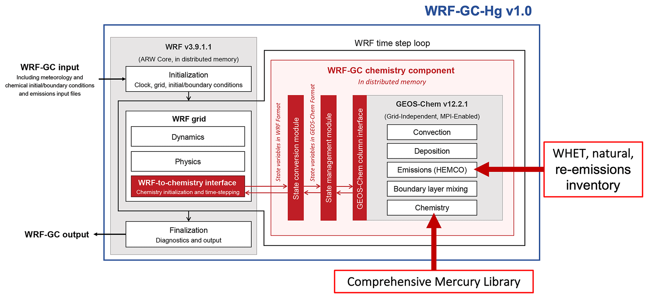

Figure 2Model simulation domain: (a) black box represents a single grid of GEOS-Chem 4∘ × 5∘ simulation, red circles represent MDN sites and triangles represent AMNet sites within this domain; (b) comparison of one cell between a resolution of 4∘ × 5∘, 50 km × 50 km, and 25 km × 25 km.
2.1 WRF-GC model with Hg
We develop a new simulation capacity (WRF-GC-Hg v1.0) for atmospheric Hg emission, transport, chemistry, and deposition based on the WRF-GC v1.0, which is fully described by Lin et al. (2020) and Feng et al. (2021). (For short, we will continue to use WRF-GC for WRF-GC-Hg v1.0 in the following paragraphs.) The model's framework is shown in Fig. 1. Briefly, the model contains three parts: the WRF mesoscale meteorological model (https://www.mmm.ucar.edu/weather-research-and-forecasting-model, last access: 28 April 2021), the GEOS-Chem global 3-D atmospheric chemistry model (http://acmg.seas.harvard.edu/geos/, last access: 28 April 2021), and the WRF-GC coupler. The WRF v3.9.1.1 (https://github.com/wrf-model/WRF/tree/V3.9.1.1, last access: 28 April 2021) Advanced Research WRF (ARW) solver is used to simulate meteorological processes and the advection of the compositions of the atmosphere with GEOS-Chem v12.2.1 (https://doi.org/10.5281/zenodo.2580198, International GEOS-Chem Community, 2019) as a self-contained chemical module. The WRF-GC coupler consists of an interface, state conversion, and management module for the two parent models. On the one hand, the WRF-GC model can take advantage of the WRF model to simulate meteorology in highly customized model domains and resolutions. In addition, the WRF offers options for configuration, vertical levels, horizontal grids, and map projections. The WRF also supplies options for land surface physics, planetary boundary layer physics, radiative transfer, cloud microphysics, and cumulus parameterization (Skamarock et al., 2008). On the other hand, the WRF-GC inherits the state-of-the-art emission, chemistry, and deposition simulation from the GEOS-Chem model (Long et al., 2015; Eastham et al., 2018). All chemical configurations, including chemical species, mechanisms, emissions, and diagnostics can be customized using the FlexChem pre-processor, a wrapper for the Kinetic PreProcessor (KPP) that allows users to add chemical species and reactions and develop their chemical mechanism (Damian et al., 2002; Sandu and Sander, 2006). The standard chemistry option of GEOS-Chem includes a full Ox–NOx–VOC–halogen–aerosol (VOC: volatile organic compound) chemistry mechanism for the troposphere that contains 208 chemical species and 981 reactions and a unified tropospheric–stratospheric chemistry extension (UCX) (Eastham et al., 2014).
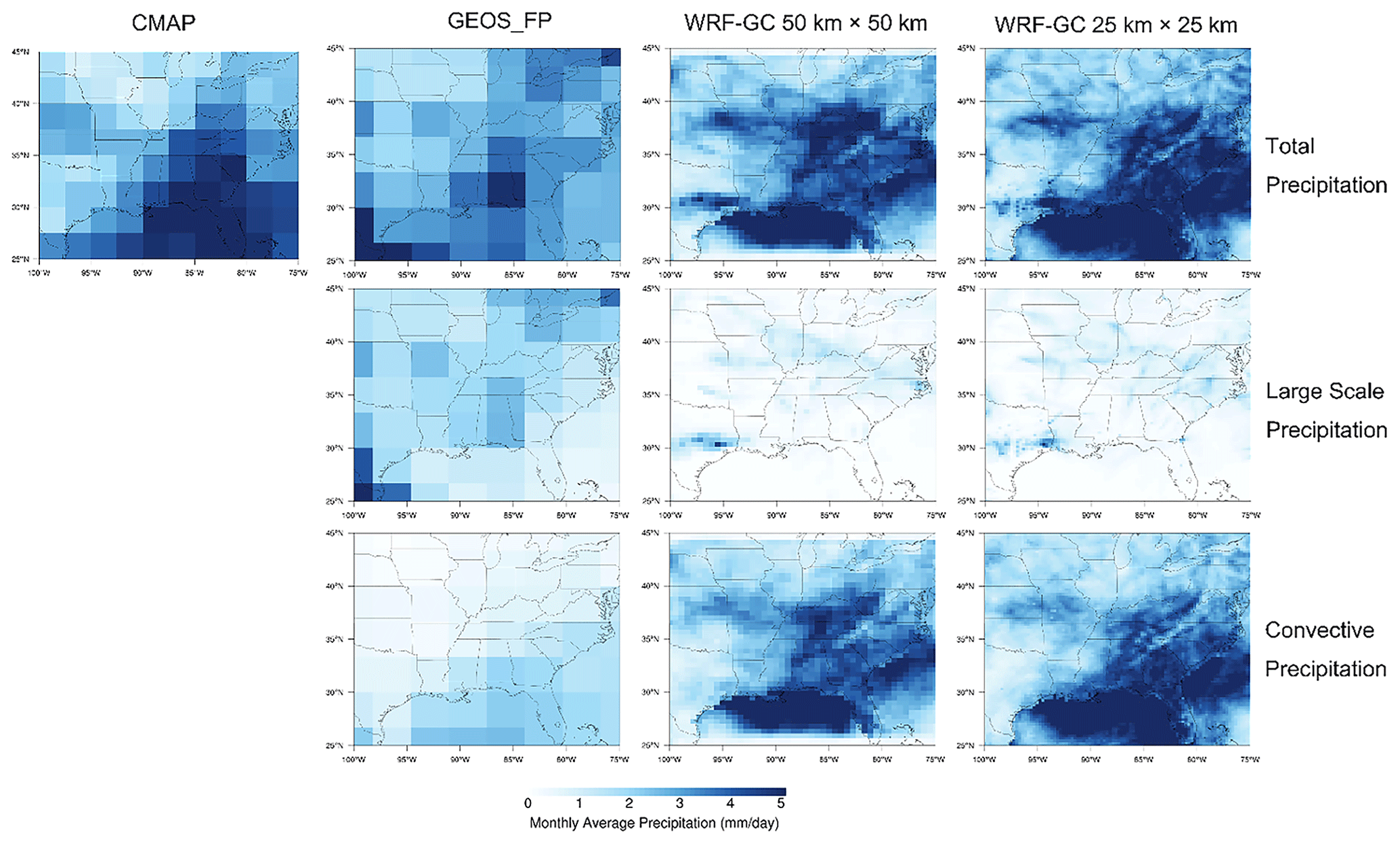
Figure 3Monthly average precipitation from July to September 2013. Left top corner: CPC Merged Analysis of Precipitation; second to fourth column: GEOS_FP offline meteorological dataset and WRF-GC precipitation at 50 km × 50 km and 25 km × 25 km resolution; from top to bottom: 3-month average precipitation, non-convective precipitation, convective precipitation.
We implement a complementary Hg chemistry library (see Fig. 1) in the WRF-GC model by first introducing Hg species to the GEOS-Chem module: Hg0 (GEM), Hg2 (GOM), HgP (PBM), and two Hg(I) species (HgBr and HgCl). The chemical reactions of Hg involve the two-stage oxidation of Hg0 to Hg(I) and Hg2 by halogens, and the reaction rates follow Horowitz et al. (2017). Similarly, the aqueous-phase reduction of GOM to Hg0 in cloud droplets and the partitioning of Hg2 and HgP on aerosols are also included. These Hg species and reactions are added to the standard GEOS-Chem KPP solver, so the concentrations of chemicals that can react with Hg (e.g., Br, BrO, OH, NO2) can be directly read online. Similar to other species in GEOS-Chem, the emissions of Hg are handled by the Harmonized Emission Component (HEMCO) (Lin et al., 2021). We use the WHET emission inventory (1∘ × 1∘) for anthropogenic Hg emissions (Zhang et al., 2016) as well as the natural emission and re-emission inventory (4∘ × 5∘) from (Horowitz et al., 2017) (see Fig. 1). The re-emissions from soil, snow, and ocean are not dynamically modeled but directly read in as a static monthly emission inventory through HEMCO based on a former GEOS-Chem Hg simulation (Horowitz et al., 2017).
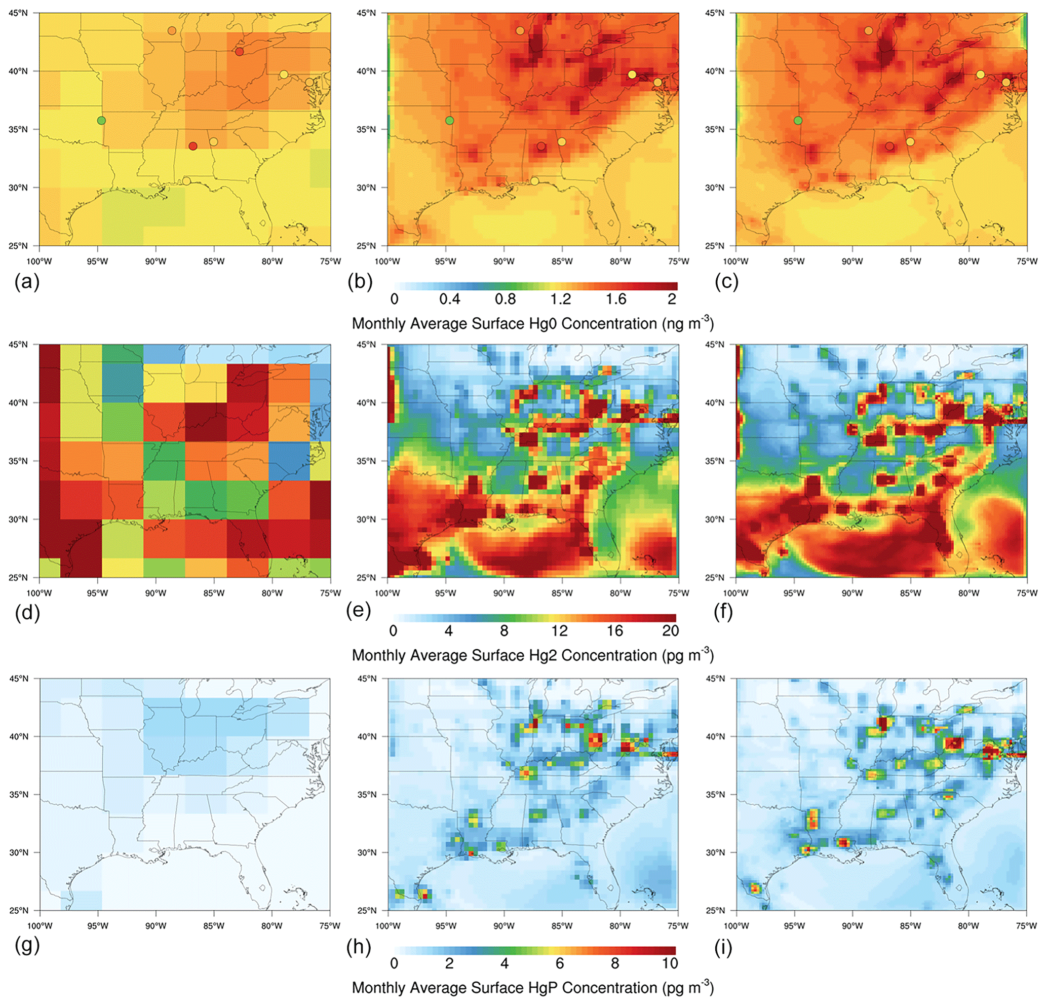
Figure 4Comparison of monthly average Hg surface concentration of Hg0 (a, b, c), Hg2 (d, e, f), and HgP (g, h, i) from July to September 2013. Panels (a, d, g) show the GEOS-Chem 4∘ × 5∘ simulation. Panels (b, e, h)–(c, f, i) correspond to different WRF-GC resolutions: 50 km × 50 km and 25 km × 25 km. Dots in (a–c) represent Hg0 observation data from AMNet of NADP (http://nadp.slh.wisc.edu/AMNet/, last access: 16 March 2021).
The WRF-GC model is a regional model that requires initial and lateral boundary conditions, which are provided by a global GEOS-Chem simulation with a consistent setup. In this study, we run the GEOS-Chem Hg simulation at 4∘ × 5∘ resolution, driven by the GEOS_FP offline meteorological dataset from the Goddard Earth Observation System (GEOS) of the NASA Global Modeling and Assimilation Office (GMAO) with 47 vertical layers. The GEOS-Chem simulation is configured to start to run a few days earlier than the WRF-GC simulation. The lateral boundary conditions of other species (e.g., Br and NO2) are also provided by a standard GEOS-Chem full chemistry simulation that is driven by the same resolution and meteorological data as the Hg simulation. The output of the GEOS-Chem Hg and full chemistry simulations are then processed and combined before being fed into the WRF-GC model.
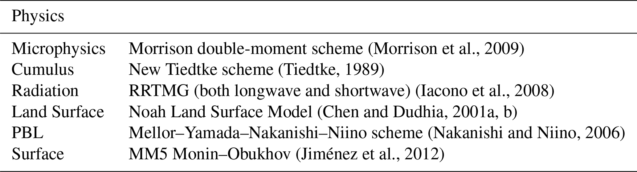
We set up a simulation domain over the southeastern US and a simulation period of July–September 2013 because convective precipitation is normally concentrated in summer (Fulkerson and Nnadi, 2006; Holmes et al., 2016). The model domain extends west–east from the middle of Texas to Pennsylvania and north–south from the Canadian border to Florida (Fig. 2). We ran simulations with different horizontal resolutions (50 km × 50 km and 25 km × 25 km for WRF-GC and 4∘ × 5∘ for GEOS-Chem) rather than using nested domains. These horizontal resolutions result in 106 × 111 grid boxes for a horizontal resolution of 25 km and 51 × 65 boxes for a resolution of 50 km. Table 1 lists the physical setup and configuration for the WRF model following Feng et al. (2021) and Lin et al. (2020). Large-scale meteorological datasets used for WRF-GC are from National Centers for Environmental Prediction (NCEP) FNL Operational Global Analysis data at 1∘ × 1∘ resolution with a 6 h interval (https://doi.org/10.5065/D6M043C6, National Centers for Environmental Prediction et al., 2020). The meteorological data and tracer advection are handled by the WRF model component, while emission, convective transport, chemistry, deposition, and boundary layer mixing are calculated by the GEOS-Chem module. These two model components exchange data online during runtime. This enables the WRF-GC Hg simulation to be run at a customized high resolution that stand-alone GEOS-Chem cannot realize. We archive hourly meteorological variables, chemical tracer concentrations, and wet-deposition fluxes of Hg2 for analysis.

Figure 5Comparison of total Hg wet deposition by different model simulations from July to September 2013. Panel (a) is GEOS-Chem 4∘ × 5∘ simulation. Panels (b) and (c) correspond to different WRF-GC resolutions: 50 km × 50 km and 25 km × 25 km. The circles represent wet deposition lower than 4 µg m−2 and rhombuses represent higher than 4 µg m−2.
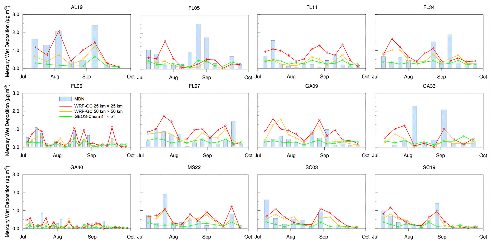
Figure 6Time series plot of comparison of MDN observation, GEOS-Chem 4∘ × 5∘, and WRF-GC 50 km × 50 km and 25 km × 25 km simulation results. This plot only shows MDN sites in Florida; a full time series plots is found in the Supplement.
Figure 3 compares the precipitation during July–September 2013 between WRF-GC at different resolutions and CPC Merged Analysis of Precipitation (CMAP) data. The CMAP is 2.5∘ × 2.5∘ monthly analyses of global precipitation, generated from merging rain gauges and several satellite-based algorithms (Xie and Arkin, 1997). The average total precipitation of WRF-GC 25 km × 25 km is 3.49 mm d−1 for the whole simulation region during 3 months in 2013, consistent with the CMAP data (3.16 mm d−1). The spatial distribution of the WRF-GC model resembles that of the CMAP data, with the highest precipitation in the northern Gulf of Mexico and extending to the nearby continental regions. The average precipitation over the southeastern-most region (25–35∘ N, 75–95∘ W) is substantially higher (4.63 mm d−1), which also agrees with the CMAP data (4.51 mm d−1). We further divide the total precipitation from the WRF-GC simulation to non-convective (or stratiform) and convective parts. The WRF-GC model suggests that convective precipitation accounts for ∼90 % of total precipitation in this region (Fig. 3).
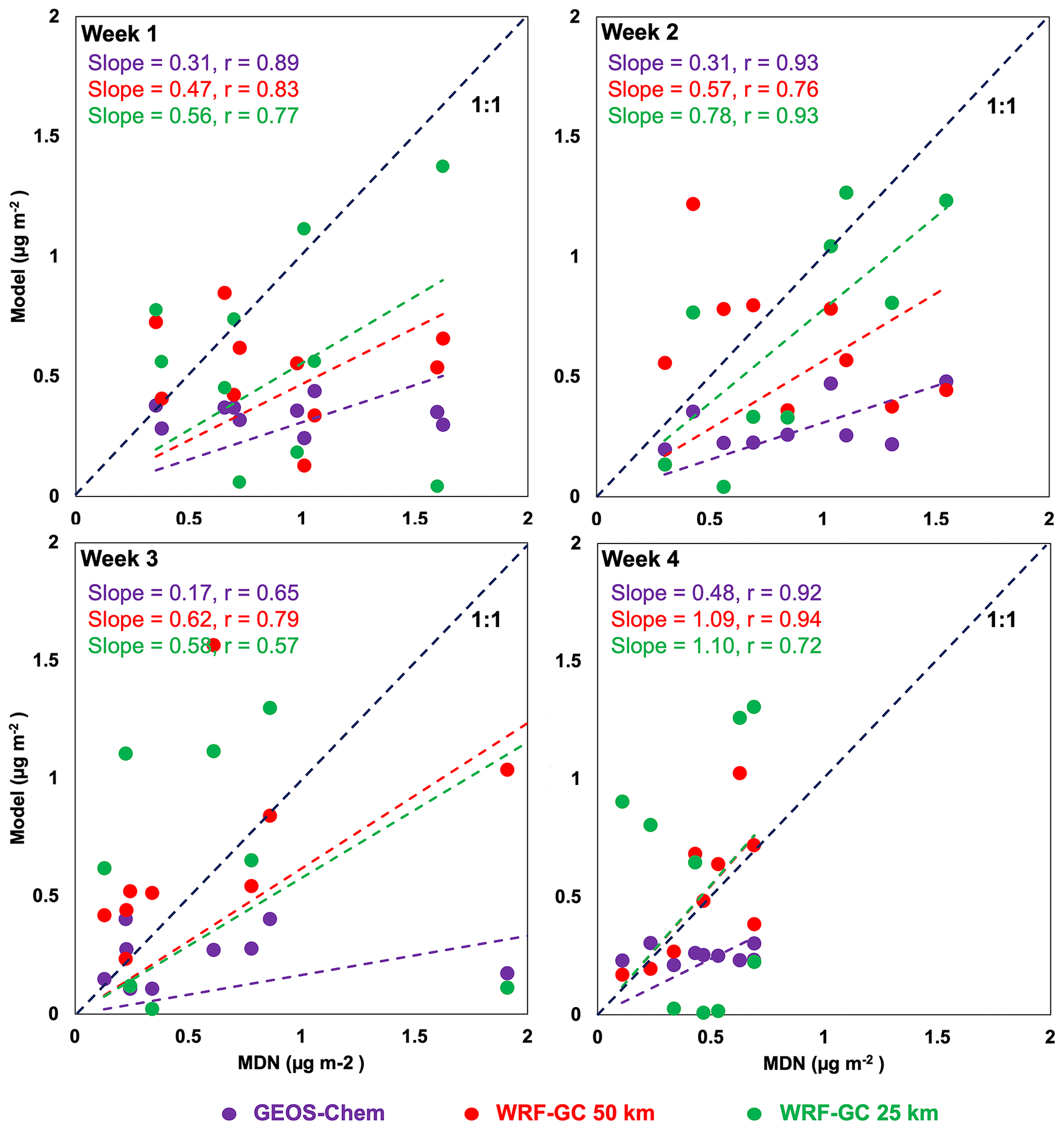
Figure 7Comparison of correlation analysis of different simulations for 4 separate weeks at 12 high-value MDN sites.
The average total precipitation of WRF-GC 25 km × 25 km is 3.49 mm d−1 for the whole simulation region, of which convective precipitation and non-convective precipitation account for 3.11 and 0.39 mm d−1. However, when the simulation narrows down to the southeastern-most region (25–35∘ N, 75–95∘ W), the average total precipitation increases to 4.63 mm d−1 and convective precipitation increases to 4.33 mm d−1, while the large-scale precipitation decreases to 0.29 mm d−1. This shows that although the southeastern region only takes up one-third of the whole simulation area, the total precipitation and convective precipitation are 32.66 % and 39.23 % higher than average, while non-convective is 25.64 % lower than the average of the whole simulation domain.
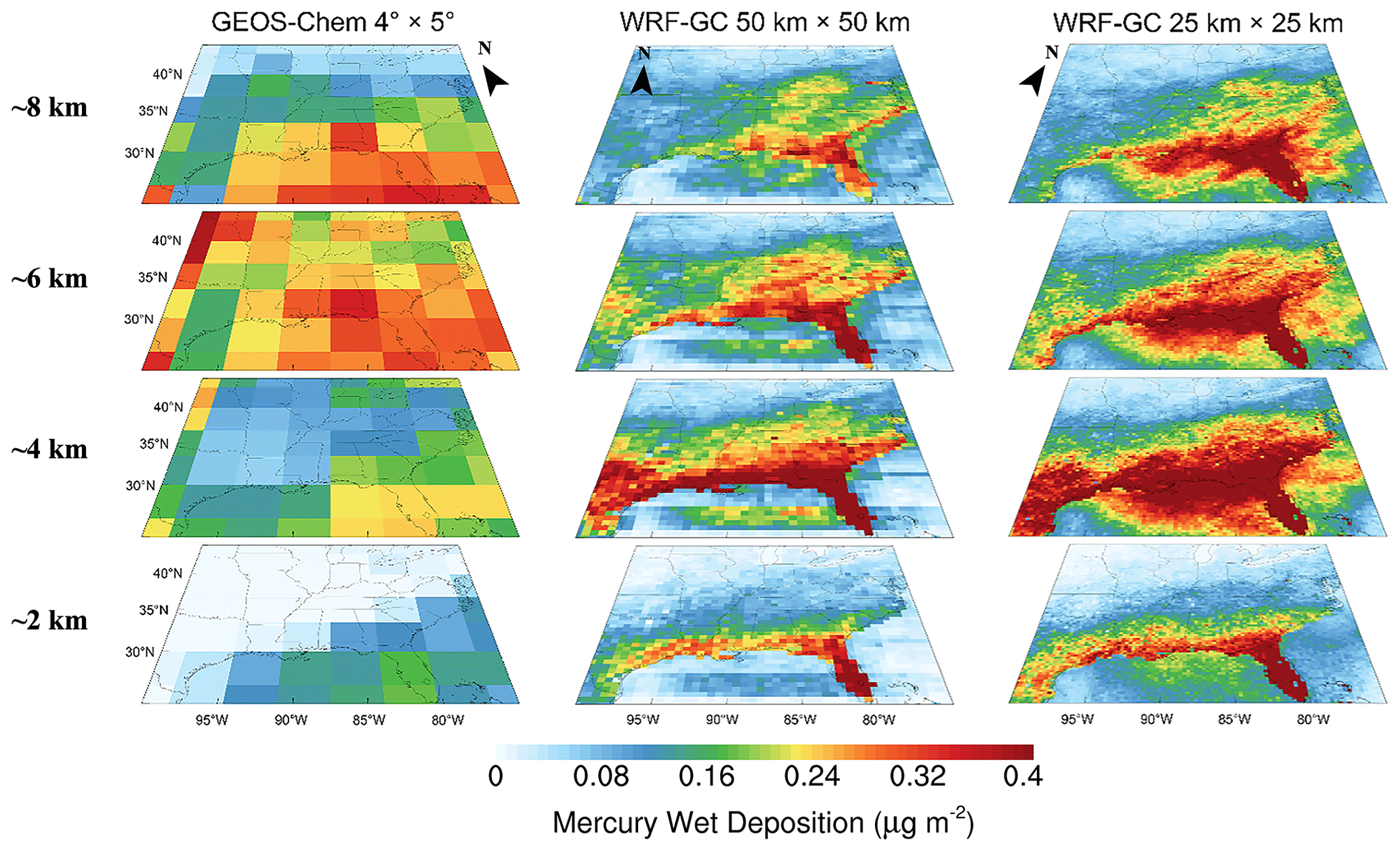
Figure 8Comparison of total Hg wet deposition of GEOS-Chem and WRF-GC at different levels and resolution. From top to bottom: the simulation results for the ∼2 km, ∼4 km, ∼6 km, and ∼8 km level, respectively. The first column is GEOS-Chem 4∘ × 5∘ simulation results. The other two from left to right correspond to different WRF-GC resolutions: 50 km × 50 km and 25 km × 25 km.
2.2 Observation data
The weekly-based Hg wet-deposition data over the MDN sites are extracted from the National Atmospheric Deposition Program (NADP) website (https://nadp.slh.wisc.edu/networks/mercury-deposition-network/, National Atmospheric Deposition Program, 2020b). The development of MDN has been described in the Introduction. During the period of this simulation, from July to September 2013, there are over 80 sites inside this domain having data. Besides, many missing values or unqualified values existed in the MDN dataset since it was collected manually. For example, the NE25 site has only three valid data points in 3 months. Hence it is important to conduct a quality check before using the data. We only take sites that have at least 75 % availability of data for 3 months (Holmes et al., 2010). After this quality check, only 55 sites are finally chosen for this study. The atmospheric Hg0 data are extracted from the Atmospheric Mercury Network (AMNet) by NADP (https://nadp.slh.wisc.edu/networks/atmospheric-mercury-network/, National Atmospheric Deposition Program, 2020a), and eight AMNet sites are chosen (see Supplement Table S2).
3.1 Comparison of mercury concentration between WRF-GC, GEOS-Chem, and AMNet
We compare the WRF-GC modeled Hg0 concentrations to AMNet observations to evaluate the model performance (Fig. 4). Due to the relatively long residence time of Hg0, the concentration distributions are relatively uniform in the model domain. The average Hg0 concentrations are 1.25 ± 0.22 ng m−3 for the eight sites in the southeast US, which agrees well with GEOS-Chem results 1.27 ± 0.06 ng m−3. The WRF-GC (1.61 ± 0.20 ng m−3) model does not agree particularly with the observations or GEOS-Chem, but it is close. This might be due to the development of WRF-GC (Hg chemistry library) coupling the GEOS-Chem full-chemistry library with the offline Br simulation. Even though all parameters were set the same as running GEOS-Chem, aqueous reductions and aerosol concentration may not be the same as GEOS-Chem's results. The WRF-GC model simulates more elevated Hg0 concentrations in the Ohio River valley regions than GEOS-Chem, by which the coarse resolution smooths out the higher anthropogenic emissions from mainly utility coal burning (Zhang et al., 2012). Similar patterns are simulated for Hg2 and HgP by WRF-GC due to their shorter residence time in the atmosphere. The influence of large point sources on nearby regions is even more distinct in WRF-GC simulations with higher resolutions, whereas the GEOS-Chem model cannot capture the hotspots of Hg2 and HgP concentrations associated with point sources, largely because it is limited by its resolution. However, both models show substantially higher near-surface Hg2 (GEOS-Chem 5.98 ± 1.94 pg m−3 and WRF-GC 13.2 ± 7.74 pg m−3 vs. AMNet 3.56 ± 6.09 pg m−3). HgP of WRF-GC (3.32 ± 2.34 pg m−3) is similar to AMNet: 3.48 ± 2.02 pg m−3 and largely higher than GEOS-Chem (0.57 ± 0.42 ng m−3). This is likely caused by the potential low sampling bias of the annular denuder coating with the potassium chloride (KCl) method (Lyman et al., 2010; Gustin et al., 2015; McClure et al., 2014) used by AMNet Hg2/HgP measurements. Zhang et al. (2012) compared to the concurrent side-by-side cation exchange membrane measurements (Lyman et al., 2020). Another possible reason is different sampling efficiencies under conditions of higher atmospheric ambient ozone and high-level relative humidity caused uncertainties for GOM (Gustin et al., 2013, 2015; Huang and Gustin, 2015; Weiss-Penzias et al., 2015).
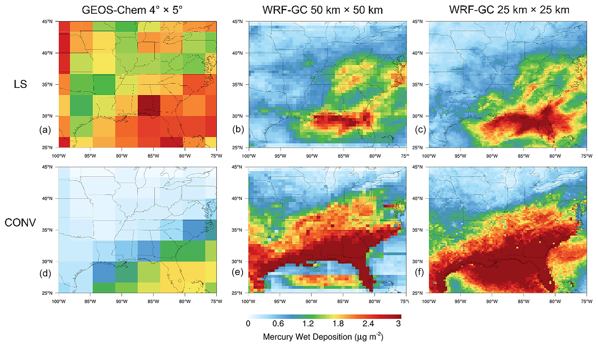
Figure 9Comparison of different types of wet deposition of GEOS-Chem and WRF-GC. Panels (a, b, c) show LS, and panels (d, e, f) show CONV. Panels (a, d) show GEOS-Chem 4∘ × 5∘ simulation results. Panels (b, e)–(c, f) correspond to different WRF-GC resolutions: 50 km × 50 km and 25 km × 25 km.
3.2 Comparison of Hg wet deposition between WRF-GC, GEOS-Chem, and MDN
Figure 5 shows the modeled Hg wet-deposition fluxes in the southeast US during July–September 2013, compared to MDN observations. We include the Hg2 and HgP wet deposition caused by both large-scale (LS or non-convective) and convective (CONV) precipitations. The GEOS-Chem model is included as a benchmark while the WRF-GC at different spatial resolutions (from 50 to 25 km) is also shown. The MDN sites observed an average of 3.27 ± 1.90 µg m−2 for all the 55 sites of the domain in the 3 months. There is a clear spatial pattern for the flux with higher deposition (6.25 ± 1.48 µg m−2) over the 12 sites in the southeastern-most part of the US (in Georgia, Alabama, Mississippi, South Carolina, and Florida) than the other 43 sites (2.44 ± 0.93 µg m−2). Both the GEOS-Chem and WRF-GC simulate similar Hg wet-deposition patterns with the observations: 0 to 3 µg m−2 in the top-left part of the simulation domain and >4 µg m−2 in areas close to the Gulf of Mexico area. However, we find a significant underestimation for these 12 sites by the GEOS-Chem model (3.33 µg m−2, 46 % lower than MDN). With higher resolutions, the modeled values increase to 2.86 ± 1.07 µg m−2 (50 km) and 4.16 ± 1.21 µg m−2 (25 km), which gradually alleviates the underestimation as the resolution increases.
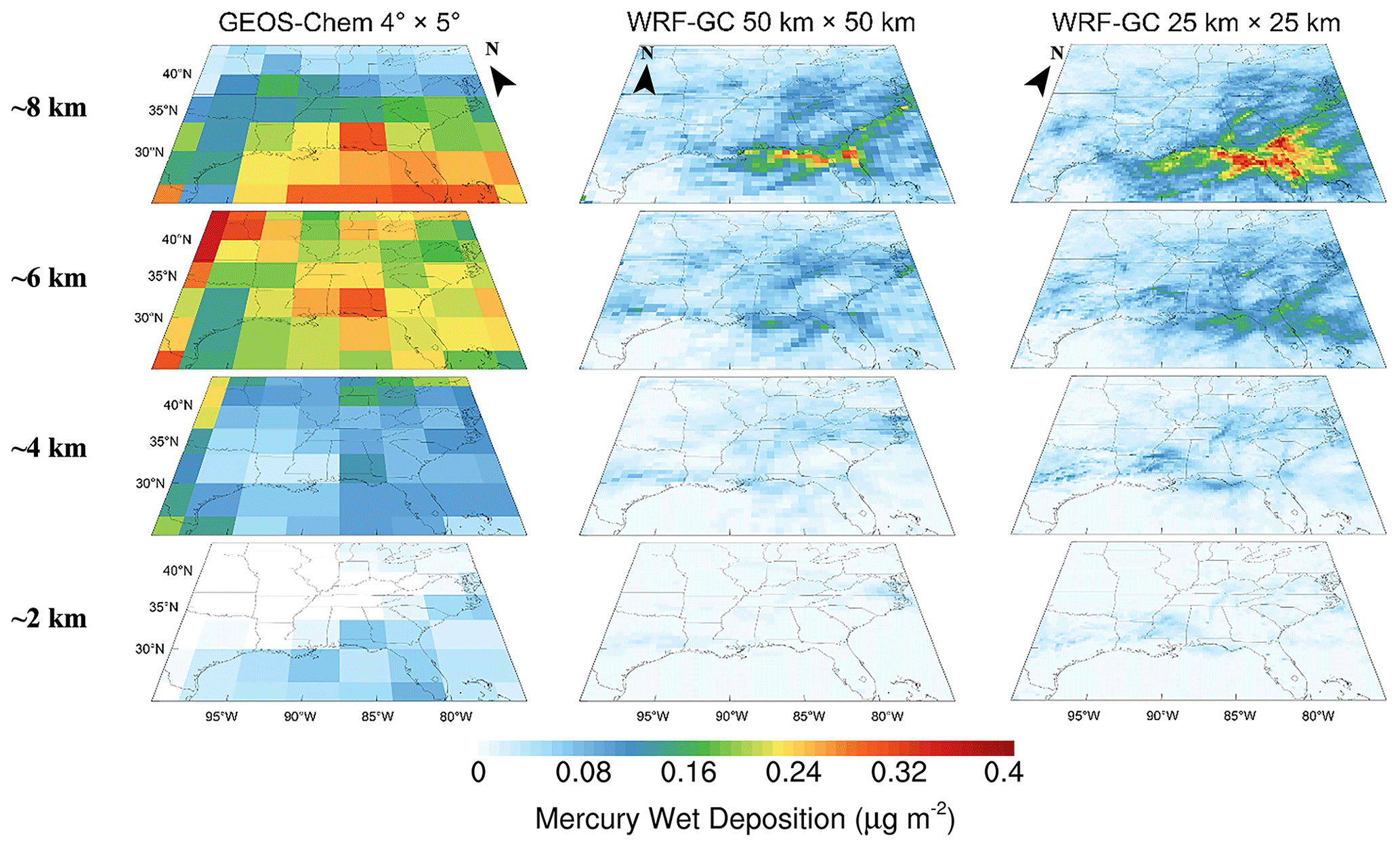
Figure 10Comparison of LS of GEOS-Chem and WRF-GC at different levels and resolutions. From top to bottom: Hg wet deposition at ∼2, ∼4, ∼6, and ∼8 km, respectively. The first column is GEOS-Chem 4∘ × 5∘ simulation results. Other columns from left to right correspond to different WRF-GC resolutions: 50 km × 50 km and 25 km × 25 km.
3.3 Week-to-week comparison of Hg wet deposition between WRF-GC, GEOS-Chem, and MDN
The MDN sites collect weekly precipitation samples, and, ideally, a total of ∼12 samples are included in the 3-month period we studied. Figure 6 compares the measured weekly Hg wet-deposition flux over the 12 sites with higher values with the GEOS-Chem and WRF-GC models with different resolutions (plots for the other sites are shown in Fig. S4 in the Supplement). We see a clear episodic pattern for the weekly samples for sites with the highest deposition fluxes. For example, the FL05 site at Florida state has a total deposition flux of 9.19 µg m−2 in the 3 months, while the largest 3 weeks (6–27 August) contribute 57 % with the other 9 weeks contributing only 43 %. Similar patterns are also observed in FL34, FL11, MS22, GA40, and SC19.
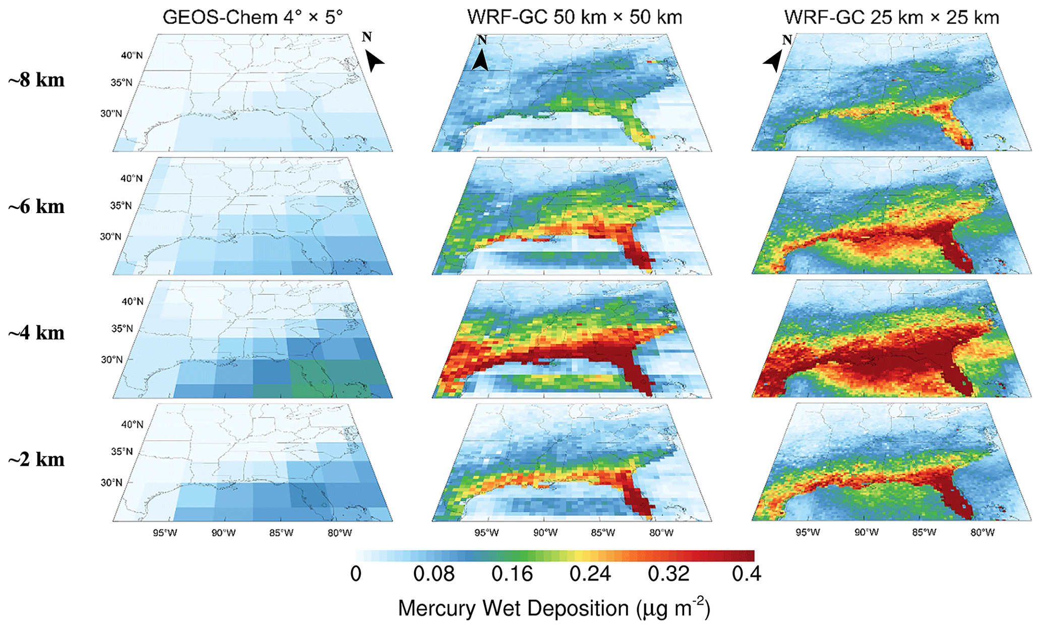
Figure 11Comparison of CONV of GEOS-Chem and WRF-GC at different levels and resolutions. From top to bottom: Hg wet deposition at ∼2, ∼4, ∼6, and ∼8 km, respectively. The first column is GEOS-Chem 4∘ × 5∘ simulation results. Other columns from left to right correspond to different WRF-GC resolutions: 50 km × 50 km and 25 km × 25 km.
Therefore, we assume that the reason for the underestimation of Hg wet deposition in GEOS-Chem is the loss of peak value. For example, the second sampling period of FL11 in Fig. 6, where MDN captures 1.54 µg m−2, both GEOS-Chem 4∘ × 5∘ and WRF-GC 50 km × 50 km simulated a value of 0.48 µg m−2, while WRF-GC 25 km × 25 km shows a value of 0.98 µg m−2. As the resolution increases, WRF-GC can better grasp the convective precipitation on a small scale than the GEOS-Chem simulation. However, we find that this increase in resolution is finite because the improvement of the increase in wet-deposition flux is not that obvious as WRF-GC resolution increases. Figure 7 shows the analysis of four short-period cases for 12 high-value MDN sites in July (week 1: 2–9; week 2: 10–16; week 3: 17–23; week 4: 24–30). From GEOS-Chem 4∘ × 5∘ to WRF-GC 50 km × 50 km (∼0.5∘), though GEOS-Chem has a better correlation coefficient for most of the time, the slope of high-resolution simulation of WRF-GC is much closer to the 1 : 1 line than GEOS-Chem simulation. This result also proves the underestimation of GEOS-Chem simulation in Hg wet deposition. As the WRF-GC resolution increases to 25 km × 25 km (∼0.25∘), the results are higher than the results from a 50 km × 50 km resolution. Here the increase in resolution is only better for the meteorology simulation because a finer resolution can help the model resolve small-scale weather conditions. Since the resolution of emission inventories is fixed (1∘ × 1∘ and 4∘ × 5∘), with higher resolution, more Hg wet deposition will be shown in our result because more convective precipitation is captured by the model.
3.4 Comparison of vertical structure of Hg wet deposition between WRF-GC and GEOS-Chem
Figure 8 shows the vertical structure of total Hg wet deposition simulated by the GEOS-Chem and WRF-GC models. Both GEOS-Chem and WRF-GC present a rising (4 km) trend first and then a falling one (8 km), with the highest values occurring at ∼6 km. Hg wet deposition only exists on the border of the Gulf of Mexico and Florida, and each model shows Florida has the highest value (GEOS-Chem: 0.2 µg m−2; WRF-GC: 0.4 µg m−2) at this level. At the height increase to ∼6 km, the distribution of Hg wet deposition becomes larger with the value of ∼0.4 µg m−2 for two models, and more places have Hg wet deposition larger than 0.4 µg m−2. When the height increases to ∼8 km, Hg wet deposition in other regions starts to fall, and only the southeastern-most areas still present higher value. Although the GEOS-Chem 4∘ × 5∘ simulation has some differences to WRF-GC 50 km × 50 km and 25 km × 25 km simulation, the whole trend and the distribution are similar. Therefore, to better understand which specific type of precipitation caused high-Hg wet deposition, we divided the total Hg wet deposition into two types: large-scale-caused Hg wet deposition (LS or non-convective) and convective-caused Hg wet deposition (CONV).
3.5 Comparison of different types of Hg wet deposition between WRF-GC and GEOS-Chem
Figure 9a–c and d–f show Hg wet deposition caused by LS and CONV, respectively. LS of GEOS-Chem is slightly higher than that of WRF-GC, but we can still clearly see the higher value of >2 µg m−2 distributed in the southeastern-most area. However, for CONV, although two models share higher Hg wet deposition in the same area, CONV of GEOS-Chem is lower than 1.8 µg m−2, whereas CONV of WRF-GC is normally higher than 3 µg m−2. Besides, we calculated the percentage of LS, CONV, and the ratio of LS / CONV from a different model. CONV in GEOS-Chem only takes 23.41 % of total Hg wet deposition in this domain, while WRF-GC has 61.54 % of Hg wet deposition resulting from CONV. The ratio of LS / CONV in GEOS-Chem is 3.27, and that in WRF-GC is 0.56. These both preliminarily verified that Hg wet deposition in the southeastern US came from convective precipitation. To further prove the height of convective precipitation that caused high-Hg wet deposition, we divided these two types of Hg wet deposition by height.
3.6 Comparison of vertical structure for different types of Hg wet deposition between WRF-GC and GEOS-Chem
Figure 10 shows Hg wet deposition by LS from GEOS-Chem and WRF-GC at different resolutions and heights. LS from both GEOS-Chem and WRF-GC increases as the height increases, and the two models all have values <0.1µg m−2 under ∼6 km. However, LS from GEOS-Chem is much larger than WRF-GC at a height of ∼6 km. We assume this might be caused by the GEOS_FP meteorological data because large-scale precipitation is stronger than WRF-GC in Fig. 2. LS at ∼8 km is the same for the two models, but as the resolution increases, the description of the distribution of the Hg wet position gets better. Figure 11 shows Hg wet deposition by CONV from GEOS-Chem and WRF-GC at different resolutions and heights. We can see the higher CONV of the two models distributed in the southeastern-most area, and it presents an increasing trend until ∼4 km and a decrease later. CONV of GEOS-Chem is lower than 0.15 µg m−2, but WRF-GC can reach 0.8 µg m−2 at ∼4 km and 0.5 µg m−2 at ∼6 km and remain at 0.3 µg m−2 at ∼8 km. Besides, by comparing the different resolutions of the WRF-GC simulation, the distribution of Hg wet deposition is getting more and more continuous. Also, because a higher resolution can capture the peak Hg wet deposition by convective precipitation in a small domain, the total Hg wet deposition slightly increases with the resolution.
This study applies a new coupled WRF-GC v1.0 model and develops comprehensive codes of Hg simulation for the model (WRF-GC-Hg v1.0) to explain the reason for higher wet deposition in the southeastern United States. Boundary conditions are provided by a global GEOS-Chem Hg simulation at a 4∘ × 5∘ resolution with the same emissions and chemistry.
Comparisons between WRF-GC simulation in 50 km × 50 km and 25 km × 25 km resolution, GEOS-Chem Hg simulation results at 4∘ × 5∘ resolution, and the observation dataset from AMNet and MDN were extensively conducted. WRF-GC simulated an average Hg0 concentration of 1.61 ± 0.20 ng m−3, which agrees with the GEOS-Chem simulation (1.27 ± 0.06 ng m−3) and the AMNet observation (1.25 ± 0.22 ng m−3). There is a large difference between the Hg2/HgP concentration from AMNet and the two models, which we suggest is caused by the potential low sampling bias of the traditional annular denuder coating with the potassium chloride method used in the AMNet Hg2/HgP measurements.
Regarding Hg wet deposition, two models have a similar distribution in the southeastern-most area, but the value of Hg wet deposition of WRF-GC (3.48 ± 2.02 µg m−2) is closer to MDN sites (3.27 ± 1.90 µg m−2) than GEOS-Chem (1.25 ± 0.22 µg m−2). Twelve sites were chosen in the southeastern-most area (in the states of Mississippi, Alabama, Georgia, South Carolina, and Florida) since higher values usually occur in this region. After analyzing time series variation, we found that Hg wet deposition came from a few short periods but was not evenly distributed in 3 months, which corresponds to the occurrence of convective precipitation.
To prove the higher Hg wet deposition came from convective precipitation at higher space, we first describe Hg wet deposition with a different model at a different height. It is clear that Hg wet deposition from the two models increases with height first and then decreases, and most of the Hg wet deposition was at a higher height. Then we divided Hg wet deposition according to different types of precipitation: large-scale and convective. LS of GEOS-Chem is slightly higher than that of WRF-GC, but we can still clearly see the higher value of >2 µg m−2 in the southeastern-most area. However, CONV of GEOS-Chem is lower than 1.8 µg m−2, while that of WRF-GC is normally higher than 3 µg m−2. Besides, the ratio of LS / CONV from GEOS-Chem is 3.27 and that of WRF-GC is 0.56 since CONV in GEOS-Chem only takes 23.41 % of total Hg wet deposition in this domain, while WRF-GC has 61.54 % of Hg wet deposition. Last, we combine the two abovementioned analyses and expand Hg wet deposition by different types of precipitation at different heights. LS from both GEOS-Chem and WRF-GC increases as the height increase, and the two models both have values <0.1 µg m−2 under ∼6 km, whilst LS from GEOS-Chem is much larger than WRF-GC at a height of ∼6 km. We assume GEOS_FP meteorological data might cause this situation. CONV from GEOS-Chem and WRF-GC are both distributed in the southeastern-most area and present an increasing trend until ∼4 km and decrease later. However, CONV of GEOS-Chem is lower than 0.15 µg m−2, whilst WRF-GC can reach 0.8 µg m−2 at ∼4 km and 0.5 µg m−2 at ∼6 km and remain at 0.3 µg m−2 at ∼8 km. This may be slightly different from previous research in that high-Hg wet deposition was scavenged by a supercell thunderstorm at a height of over 10 km.
In addition, by comparing the different resolutions of the WRF-GC simulation, the distribution of Hg wet deposition is becomes more and more continuous. Also, because a higher resolution can capture the peak Hg wet deposition by convective precipitation in a small domain, the total Hg wet deposition slightly increases with the resolution. However, we need to notice that the increase in simulation performance with an increase in resolution is finite.
The parent WRF-GC v1.0 model is open source and can be downloaded from GitHub (https://github.com/jimmielin/wrf-gc-release/tree/v0.9, last access: 28 April 2021) or in Zenodo at https://doi.org/10.5281/zenodo.3550330, (Lin et al., 2019). The code and data used for implementing mercury into WRF-GC (WRF-GC-Hg v1.0) in this paper can be obtained from GitHub (https://github.com/Jim-Xu/WRF-GC-Hg, last access: 17 March 2022). The latest WRF-GC-Hg v1.0 is permanently archived at https://doi.org/10.5281/zenodo.6366777 (Xu and Zhang, 2022).
The supplement related to this article is available online at: https://doi.org/10.5194/gmd-15-3845-2022-supplement.
YZ supervised and guided the whole project, XX did all simulations, analysis, and paper writing, XF, HL, and TMF provided ample technical advice during the code development, and PZ, SH, ZS, and YP provided advice and assistance in analyzing results.
The contact author has declared that neither they nor their co-authors have any competing interests.
Publisher’s note: Copernicus Publications remains neutral with regard to jurisdictional claims in published maps and institutional affiliations.
The WRF project is supported and maintained by the National Center for Atmospheric Research (NCAR), and the GEOS-Chem project is supported by Harvard University. We would like to express out thanks for all scientists' and engineers' contributions to these projects. We also would like to thank Nanjing University’s High Performance Computing Center for providing computational sources for this project.
This research has been supported by the National Key Research and Development Program of China (grant no. 2019YFA0606803), the Fundamental Research Funds for the Central Universities (grant no. 0207-14380168), and the Frontiers Science Center for Critical Earth Material Cycling.
This paper was edited by Havala Pye and reviewed by two anonymous referees.
Ariya, P. A., Amyot, M., Dastoor, A., Deeds, D., Feinberg, A., Kos, G., Poulain, A., Ryjkov, A., Semeniuk, K., Subir, M., and Toyota, K.: Mercury Physicochemical and Biogeochemical Transformation in the Atmosphere and at Atmospheric Interfaces: A Review and Future Directions, Chem. Rev., 115, 3760–3802, https://doi.org/10.1021/cr500667e, 2015.
Brisson, E., Van Weverberg, K., Demuzere, M., Devis, A., Saeed, S., Stengel, M., and van Lipzig, N. P. M.: How well can a convection-permitting climate model reproduce decadal statistics of precipitation, temperature and cloud characteristics?, Clim. Dynam., 47, 3043–3061, https://doi.org/10.1007/s00382-016-3012-z, 2016.
Bullock, O. R. and Brehme, K. A.: Atmospheric mercury simulation using the CMAQ model: formulation description and analysis of wet deposition results, Atmos. Environ., 36, 2135–2146, https://doi.org/10.1016/S1352-2310(02)00220-0, 2002.
Chen, F. and Dudhia, J.: Coupling an advanced land surface-hydrology model with the Penn-State-NCAR MM5 modeling system. Part II: Preliminary model validation, Mon. Weather Rev., 129, 587–604, https://doi.org/10.1175/1520-0493(2001)129<0587:CAALSH>2.0.CO;2, 2001a.
Chen, F. and Dudhia, J.: Coupling and advanced land surface-hydrology model with the Penn State-NCAR MM5 modeling system. Part I: Model implementation and sensitivity, Mon. Weather Rev., 129, 569–585, https://doi.org/10.1175/1520-0493(2001)129<0569:CAALSH>2.0.CO;2, 2001b.
Coburn, S., Dix, B., Edgerton, E., Holmes, C. D., Kinnison, D., Liang, Q., ter Schure, A., Wang, S., and Volkamer, R.: Mercury oxidation from bromine chemistry in the free troposphere over the southeastern US, Atmos. Chem. Phys., 16, 3743–3760, https://doi.org/10.5194/acp-16-3743-2016, 2016.
Damian, V., Sandu, A., Damian, M., Potra, F., and Carmichael, G. R.: The kinetic preprocessor KPP – A software environment for solving chemical kinetics, Comput. Chem. Eng., 26, 1567–1579, https://doi.org/10.1016/S0098-1354(02)00128-X, 2002.
Eastham, S. D., Weisenstein, D. K., and Barrett, S. R. H.: Development and evaluation of the unified tropospheric-stratospheric chemistry extension (UCX) for the global chemistry-transport model GEOS-Chem, Atmos. Environ., 89, 52–63, https://doi.org/10.1016/j.atmosenv.2014.02.001, 2014.
Eastham, S. D., Long, M. S., Keller, C. A., Lundgren, E., Yantosca, R. M., Zhuang, J., Li, C., Lee, C. J., Yannetti, M., Auer, B. M., Clune, T. L., Kouatchou, J., Putman, W. M., Thompson, M. A., Trayanov, A. L., Molod, A. M., Martin, R. V., and Jacob, D. J.: GEOS-Chem High Performance (GCHP v11-02c): a next-generation implementation of the GEOS-Chem chemical transport model for massively parallel applications, Geosci. Model Dev., 11, 2941–2953, https://doi.org/10.5194/gmd-11-2941-2018, 2018.
Feng, X., Lin, H., Fu, T.-M., Sulprizio, M. P., Zhuang, J., Jacob, D. J., Tian, H., Ma, Y., Zhang, L., Wang, X., Chen, Q., and Han, Z.: WRF-GC (v2.0): online two-way coupling of WRF (v3.9.1.1) and GEOS-Chem (v12.7.2) for modeling regional atmospheric chemistry–meteorology interactions, Geosci. Model Dev., 14, 3741–3768, https://doi.org/10.5194/gmd-14-3741-2021, 2021.
Fu, X., Yang, X., Lang, X., Zhou, J., Zhang, H., Yu, B., Yan, H., Lin, C.-J., and Feng, X.: Atmospheric wet and litterfall mercury deposition at urban and rural sites in China, Atmos. Chem. Phys., 16, 11547–11562, https://doi.org/10.5194/acp-16-11547-2016, 2016.
Fulkerson, M. and Nnadi, F. N.: Predicting mercury wet deposition in Florida: A simple approach, Atmos. Environ., 40, 3962–3968, https://doi.org/10.1016/j.atmosenv.2006.02.028, 2006.
Gencarelli, C. N., de Simone, F., Hedgecock, I. M., Sprovieri, F., and Pirrone, N.: Development and application of a regional-scale atmospheric mercury model based on WRF/Chem: A Mediterranean area investigation, Environ. Sci. Pollut. R., 21, 4095–4109, https://doi.org/10.1007/s11356-013-2162-3, 2014.
Gonzalez-Raymat, H., Liu, G., Liriano, C., Li, Y., Yin, Y., Shi, J., Jiang, G., and Cai, Y.: Elemental mercury: Its unique properties affect its behavior and fate in the environment, Environ. Pollut., 229, 69–86, https://doi.org/10.1016/j.envpol.2017.04.101, 2017.
Guentzel, J. L., Landing, W. M., Gill, G. A., and Pollman, C. D.: Processes influencing rainfall deposition of mercury in Florida, Environ. Sci. Technol., 35, 863–873, https://doi.org/10.1021/es001523+, 2001.
Gustin, M. S., Huang, J., Miller, M. B., Peterson, C., Jaffe, D. A., Ambrose, J., Finley, B. D., Lyman, S. N., Call, K., Talbot, R., Feddersen, D., Mao, H., and Lindberg, S. E.: Do we understand what the mercury speciation instruments are actually measuring? Results of RAMIX, Environ. Sci. Technol., 47, 7295–7306, https://doi.org/10.1021/es3039104, 2013.
Gustin, M. S., Amos, H. M., Huang, J., Miller, M. B., and Heidecorn, K.: Measuring and modeling mercury in the atmosphere: a critical review, Atmos. Chem. Phys., 15, 5697–5713, https://doi.org/10.5194/acp-15-5697-2015, 2015.
Holmes, C. D., Jacob, D. J., Corbitt, E. S., Mao, J., Yang, X., Talbot, R., and Slemr, F.: Global atmospheric model for mercury including oxidation by bromine atoms, Atmos. Chem. Phys., 10, 12037–12057, https://doi.org/10.5194/acp-10-12037-2010, 2010.
Holmes, C. D., Krishnamurthy, N. P., Caffrey, J. M., Landing, W. M., Edgerton, E. S., Knapp, K. R., and Nair, U. S.: Thunderstorms increase mercury wet deposition, Environ. Sci. Technol., 50, 9343–9350, https://doi.org/10.1021/acs.est.6b02586, 2016.
Horowitz, H. M., Jacob, D. J., Zhang, Y., Dibble, T. S., Slemr, F., Amos, H. M., Schmidt, J. A., Corbitt, E. S., Marais, E. A., and Sunderland, E. M.: A new mechanism for atmospheric mercury redox chemistry: implications for the global mercury budget, Atmos. Chem. Phys., 17, 6353–6371, https://doi.org/10.5194/acp-17-6353-2017, 2017.
Huang, J. and Gustin, M. S.: Uncertainties of gaseous oxidized mercury measurements using KCL-coated denuders, cation-exchange membranes, and nylon membranes: Humidity influences, Environ. Sci. Technol., 49, 6102–6108, https://doi.org/10.1021/acs.est.5b00098, 2015.
Iacono, M. J., Delamere, J. S., Mlawer, E. J., Shephard, M. W., Clough, S. A., and Collins, W. D.: Radiative forcing by long-lived greenhouse gases: Calculations with the AER radiative transfer models, J. Geophys. Res., 113, 2–9, https://doi.org/10.1029/2008JD009944, 2008.
International GEOS-Chem Community: geoschem/geos-chem: GEOS-Chem 12.2.1 (Version 12.2.1), Zenodo [code], https://doi.org/10.5281/zenodo.2580198, 2019.
Jiménez, P. A., Dudhia, J., González-Rouco, J. F., Navarro, J., Montávez, J. P., and García-Bustamante, E.: A revised scheme for the WRF surface layer formulation, Mon. Weather Rev., 140, 898–918, https://doi.org/10.1175/MWR-D-11-00056.1, 2012.
Kaulfus, A. S., Nair, U., Holmes, C. D., and Landing, W. M.: Mercury Wet Scavenging and Deposition Differences by Precipitation Type, Environ. Sci. Technol., 51, 2628–2634, https://doi.org/10.1021/acs.est.6b04187, 2017.
Lin, H., Feng, X., Fu, T.-M., Tian, H., Ma, Y., Zhang, L., Jacob, D. J., Yantosca, R. M., Sulprizio, M. P., Lundgren, E. W., Zhuang, J., Zhang, Q., Lu, X., Zhang, L., Shen, L., Guo, J., Eastham, S. D., and Keller, C. A.: WRF-GC v1.0, Zenodo [code], https://doi.org/10.5281/zenodo.3550330, 2019.
Lin, H., Feng, X., Fu, T.-M., Tian, H., Ma, Y., Zhang, L., Jacob, D. J., Yantosca, R. M., Sulprizio, M. P., Lundgren, E. W., Zhuang, J., Zhang, Q., Lu, X., Zhang, L., Shen, L., Guo, J., Eastham, S. D., and Keller, C. A.: WRF-GC (v1.0): online coupling of WRF (v3.9.1.1) and GEOS-Chem (v12.2.1) for regional atmospheric chemistry modeling – Part 1: Description of the one-way model, Geosci. Model Dev., 13, 3241–3265, https://doi.org/10.5194/gmd-13-3241-2020, 2020.
Lin, H., Jacob, D. J., Lundgren, E. W., Sulprizio, M. P., Keller, C. A., Fritz, T. M., Eastham, S. D., Emmons, L. K., Campbell, P. C., Baker, B., Saylor, R. D., and Montuoro, R.: Harmonized Emissions Component (HEMCO) 3.0 as a versatile emissions component for atmospheric models: application in the GEOS-Chem, NASA GEOS, WRF-GC, CESM2, NOAA GEFS-Aerosol, and NOAA UFS models, Geosci. Model Dev., 14, 5487–5506, https://doi.org/10.5194/gmd-14-5487-2021, 2021.
Long, M. S., Yantosca, R., Nielsen, J. E., Keller, C. A., da Silva, A., Sulprizio, M. P., Pawson, S., and Jacob, D. J.: Development of a grid-independent GEOS-Chem chemical transport model (v9-02) as an atmospheric chemistry module for Earth system models, Geosci. Model Dev., 8, 595–602, https://doi.org/10.5194/gmd-8-595-2015, 2015.
Lyman, S. N. and Jaffe, D. A.: Formation and fate of oxidized mercury in the upper troposphere and lower stratosphere, Nat. Geosci., 5, 114–117, https://doi.org/10.1038/ngeo1353, 2012.
Lyman, S. N., Jaffe, D. A., and Gustin, M. S.: Release of mercury halides from KCl denuders in the presence of ozone, Atmos. Chem. Phys., 10, 8197–8204, https://doi.org/10.5194/acp-10-8197-2010, 2010.
Lyman, S. N., Gratz, L. E., Dunham-Cheatham, S. M., Gustin, M. S., and Luippold, A.: Improvements to the Accuracy of Atmospheric Oxidized Mercury Measurements, Environ. Sci. Technol., 54, 13379–13388, https://doi.org/10.1021/acs.est.0c02747, 2020.
Mason, R. P., Lawson, N. M., and Sheu, G. R.: Annual and seasonal trends in mercury deposition in Maryland, Atmos. Environ., 34, 1691–1701, https://doi.org/10.1016/S1352-2310(99)00428-8, 2000.
McClure, C. D., Jaffe, D. A., and Edgerton, E. S.: Evaluation of the KCl denuder method for gaseous oxidized mercury using HgBr2 at an in-service AMNet site, Environ. Sci. Technol., 48, 11437–11444, https://doi.org/10.1021/es502545k, 2014.
Morrison, H., Thompson, G., and Tatarskii, V.: Impact of cloud microphysics on the development of trailing stratiform precipitation in a simulated squall line: Comparison of one- and two-moment schemes, Mon. Weather Rev., 137, 991–1007, https://doi.org/10.1175/2008MWR2556.1, 2009.
Nakanishi, M. and Niino, H.: An improved Mellor-Yamada Level-3 model: Its numerical stability and application to a regional prediction of advection fog, Bound-Lay. Meteorol., 119, 397–407, https://doi.org/10.1007/s10546-005-9030-8, 2006.
National Atmospheric Deposition Program: Atmospheric Mercury Network (AMNet): A NADP Network [data set], https://nadp.slh.wisc.edu/networks/atmospheric-mercury-network/, 2020a.
National Atmospheric Deposition Program: Mercury Deposition Network (MDN): A NADP Network [data set], https://nadp.slh.wisc.edu/networks/mercury-deposition-network/, 2020b.
National Atmospheric Deposition Program: National Trends Network (NTN): A NADP Network [data set], https://nadp.slh.wisc.edu/networks/national-trends-network/, 2020c.
National Centers for Environmental Prediction, National Weather Service, NOAA, and U.S. Department of Commerce: NCEP FNL Operational Model Global Tropospheric Analyses, continuing from July 1999, Research Data Archive at the National Center for Atmospheric Research, Computational and Information Systems Laboratory, https://doi.org/10.5065/D6M043C6, 2000.
Pan, L., Lin, C. J., Carmichael, G. R., Streets, D. G., Tang, Y., Woo, J. H., Shetty, S. K., Chu, H. W., Ho, T. C., Friedli, H. R., and Feng, X.: Study of atmospheric mercury budget in East Asia using STEM-Hg modeling system, Sci. Total Environ., 408, 3277–3291, https://doi.org/10.1016/j.scitotenv.2010.04.039, 2010.
Prestbo, E. M. and Gay, D. A.: Wet deposition of mercury in the U.S. and Canada, 1996–2005: Results and analysis of the NADP mercury deposition network (MDN), Atmos. Environ., 43, 4223–4233, https://doi.org/10.1016/j.atmosenv.2009.05.028, 2009.
Rumbold, D. G., Axelrad, D. M., and Pollman, C. D.: Mercury and the everglades. A synthesis and model for complex ecosystem restoration, 1–273 pp., https://doi.org/10.1007/978-3-030-32057-7, ISBN 978-3-030-32057-7, Springer, 2019.
Sandu, A. and Sander, R.: Technical note: Simulating chemical systems in Fortran90 and Matlab with the Kinetic PreProcessor KPP-2.1, Atmos. Chem. Phys., 6, 187–195, https://doi.org/10.5194/acp-6-187-2006, 2006.
Selin, N. E., Javob, D. J., Park, R. J., Yantosca, R. M., Strode, S., Jaeglé, L., and Jaffe, D.: Chemical cycling and deposition of atmospheric mercury: Global constraints from observations, J. Geophys. Res., 112, 1–14, https://doi.org/10.1029/2006JD007450, 2007.
Selin, N. E., Jacob, D. J., Yantosca, R. M., Strode, S., Jaeglé, L., and Sunderland, E. M.: Global 3-D land-ocean-atmosphere model for mercury: Present-day versus preindustrial cycles and anthropogenic enrichment factors for deposition, Global Biogeochem. Cy., 22, 1–13, https://doi.org/10.1029/2007GB003040, 2008.
Sexauer Gustin, M., Weiss-Penzias, P. S., and Peterson, C.: Investigating sources of gaseous oxidized mercury in dry deposition at three sites across Florida, USA, Atmos. Chem. Phys., 12, 9201–9219, https://doi.org/10.5194/acp-12-9201-2012, 2012.
Skamarock, W. C., Klemp, J. B., Dudhia, J., Gill, D. O., Barker, D. M., Duda, M. G., Huang, X.-Y., Wang, W., and Powers, J. G.: A Description of the Advanced Research WRF Model Version 3, University Corporation for Atmospheric Research, 113, https://doi.org/10.5065/D68S4MVH, 2008.
Tiedtke, M: A comprehensive Mass Flux Scheme for Cumulus Parameterization in Large-Scale Models, Mon. Weather Rev., 117, 1779–1800, https://doi.org/10.1175/1520-0493(1989)117<1779:ACMFSF>2.0.CO;2, 1989.
Weiss-Penzias, P., Amos, H. M., Selin, N. E., Gustin, M. S., Jaffe, D. A., Obrist, D., Sheu, G.-R., and Giang, A.: Use of a global model to understand speciated atmospheric mercury observations at five high-elevation sites, Atmos. Chem. Phys., 15, 1161–1173, https://doi.org/10.5194/acp-15-1161-2015, 2015.
Xie, P. and Arkin, P. A.: Global Precipitation: A 17-Year Monthly Analysis Based on Gauge Observations, Satellite Estimates, and Numerical Model Outputs, Bull Am Meteorol Soc, B. Am. Meteorol. Soc., 78, 2539–2558, https://doi.org/10.1175/1520-0477(1997)078<2539:GPAYMA>2.0.CO;2, 1997.
Xu, X. and Zhang, Y.: Jim-Xu/WRF-GC-Hg: (v1.0.1), Zenodo [code and data set], https://doi.org/10.5281/zenodo.6366777, 2022.
Zhang, Y., Jaeglé, L., van Donkelaar, A., Martin, R. V., Holmes, C. D., Amos, H. M., Wang, Q., Talbot, R., Artz, R., Brooks, S., Luke, W., Holsen, T. M., Felton, D., Miller, E. K., Perry, K. D., Schmeltz, D., Steffen, A., Tordon, R., Weiss-Penzias, P., and Zsolway, R.: Nested-grid simulation of mercury over North America, Atmos. Chem. Phys., 12, 6095–6111, https://doi.org/10.5194/acp-12-6095-2012, 2012.
Zhang, Y., Jacob, D. J., Horowitz, H. M., Chen, L., Amos, H. M., Krabbenhoft, D. P., Slemr, F., St. Louis, V. L., and Sunderland, E. M.: Observed decrease in atmospheric mercury explained by global decline in anthropogenic emissions, P. Natl. Acad. Sci. USA, 113, 526–531, https://doi.org/10.1073/pnas.1516312113, 2016.