the Creative Commons Attribution 4.0 License.
the Creative Commons Attribution 4.0 License.
 | 05 May 2022
Earth system modeling of mercury using CESM2 – Part 1: Atmospheric model CAM6-Chem/Hg v1.0
Peng Zhang
Most global atmospheric mercury models use offline and reanalyzed meteorological fields, which has the advantages of higher accuracy and lower computational cost compared to online models. However, these meteorological products need past and/or near-real-time observational data and cannot predict the future. Here, we use an atmospheric component with tropospheric and stratospheric chemistry (CAM6-Chem) of the state-of-the-art global climate model CESM2, adding new species of mercury and simulating atmospheric mercury cycling. Our results show that the newly developed online model is able to simulate the observed spatial distribution of total gaseous mercury (TGM) in both polluted and non-polluted regions with high correlation coefficients in eastern Asia (r=0.67) and North America (r=0.57). The calculated lifetime of TGM against deposition is 5.3 months and reproduces the observed interhemispheric gradient of TGM with a peak value at northern mid-latitudes. Our model reproduces the observed spatial distribution of HgII wet deposition over North America (r=0.80) and captures the magnitude of maximum in the Florida Peninsula. The simulated wet deposition fluxes in eastern Asia present a spatial distribution pattern of low in the northwest and high in the southeast. The online model is in line with the observed seasonal variations of TGM at northern mid-latitudes as well as the Southern Hemisphere, which shows lower amplitude. We further go into the factors that affect the seasonal variations of atmospheric mercury and find that both Hg0 dry deposition and HgII dry/wet depositions contribute to it.
- Article
(6056 KB) - Full-text XML
-
Supplement
(651 KB) - BibTeX
- EndNote


Mercury (Hg) is a global pollutant that can be transported and exchanged among the atmosphere, geosphere, hydrosphere, cryosphere, and biosphere (Selin, 2009; Driscoll et al., 2013). Although the anthropogenic emissions are mainly to the atmosphere, most human exposure for the general population to its toxic form (methylmercury) is mainly through consumption of seafood and rice (Zhang et al., 2010; Mahaffey et al., 2011; Zhang et al., 2021). Understanding the relationship between anthropogenic emissions and human exposure requires a holistic view of the global Hg cycle, and an Earth system model that integrates the multiple spheres is required. As the first step of this effort, here we develop a new online atmospheric Hg model (CAM6-Chem/Hg v1.0, hereinafter referred to “CAM6-Chem/Hg”) within the Community Earth System Model version 2 (CESM2).
One advantage of our online model is that the concentrations of Hg oxidants are calculated online. There are three main stable forms of atmospheric mercury: gaseous elemental mercury (Hg0), reactive gaseous mercury (Hg2), and particulate bound mercury (HgP). Up to now, several Hg0 oxidants have been proposed and the debate about which is the dominant oxidant has focused on O3, OH radical, or halogen species (Si and Ariya, 2018; Lyman et al., 2020). In the previous global modeling studies, using Br as the only oxidation pathway (Holmes et al., 2010; Amos et al., 2012; Horowitz et al., 2017) or oxidation by (Selin et al., 2007; De Simone et al., 2014; Pacyna et al., 2016) can both get reasonable results. Nevertheless, recent studies seemed to indicate that more complex chemistry and multiple oxidants of Hg0 exist in the atmosphere (Weiss-Penzias et al., 2015; Travnikov et al., 2017; Si and Ariya, 2018; Lyman et al., 2020; Shah et al., 2021). Previous models often use archived monthly mean concentrations for these oxidants (e.g., Seigneur et al., 2001; Durnford et al., 2012; Shah et al., 2021), which neglects the diurnal variation of these species. Similar to the meteorological data, using offline oxidants also lacks the predicting capacity for the oxidizing power of the atmosphere under future emission and climate conditions.
The other advantage of our model is that the meteorological fields are calculated online and coupled with chemistry. So far, most of the global atmospheric Hg models are offline models, such as GLEMOS (Travnikov and Ilyin, 2009), GEOS-Chem-Hg (Selin et al., 2007), CAM-Chem/Hg (Lei et al., 2013), and CTM-Hg (Seigneur et al., 2001). These offline chemical transport models (CTMs) are driven by the meteorological reanalysis data which are derived from external numerical weather prediction (NWP) or climate models. Advantages of the assimilated meteorological data include accuracy and relatively low computational cost (El-Harbawi, 2013). However, one drawback for the atmospheric chemistry models that rely on it is the lack of future data. The inputted meteorological data often need to be interpolated in time and space, and the physical parameterizations (e.g., advection and convection) are commonly different between CTMs and NWP, leading to inconsistency in the modeling results (Grell and Baklanov, 2011). The interaction between meteorology and atmospheric chemistry is also often not considered in these models. In our model, no interpolation in time or space for the meteorological data is needed, the same numerical schemes make the online model more consistent than the offline model, and the impact of meteorology and chemistry feedback can also be taken into account (Baklanov et al., 2014). Furthermore, the online Hg model is of great significance to forecast or simulate the impacts of future climate change on Hg.
We add atmospheric Hg species in the Community Atmosphere Model version 6 with chemistry (CAM6-Chem), which does not include any Hg species. The related processes such as anthropogenic and natural emissions, dry and wet deposition, and redox chemistry of Hg are also included. The CAM-Chem model has been widely used for simulations of global tropospheric and stratospheric atmospheric composition, such as OH (Wang et al., 2020), O3 (Emmons et al., 2020), and halogens (Fernandez et al., 2019). Lei et al. (2013) also developed an offline CAM-Chem/Hg model under the Community Climate System Model version 3 (CCSM3), which is the predecessor and has been greatly improved by the CESM2 used in this study. We run the CAM6-Chem/Hg model in the free-running configuration, which provides a platform for online modeling of different atmospheric Hg species. The main objective of this study is to test the performance of the model driven by online meteorology data for Hg by extensively comparing the model results with available observations worldwide.
2.1 CAM6-Chem model
The CAM6-Chem, based on the Community Atmosphere Model version 6 (CAM6), is the atmospheric component with chemistry of the CESM2 (Emmons et al., 2020). The CESM2 is an open-source community coupled model, consisting of seven major prognostic components: atmosphere, land, land–ice, ocean, sea–ice, river runoff, and wave (Danabasoglu et al., 2020). The CAM6 uses the same finite volume (FV) dynamic core (Lin and Rood, 1997) as its predecessors CCSM4 and CESM1 but with a variety of modifications (see Danabasoglu et al., 2020, for more details). The CAM6 model version we used here has a horizontal resolution of 0.9∘ in latitude by 1.25∘ in longitude, with 32 vertical levels from the surface to 2 hPa (about 45 km).
The atmospheric chemical mechanism of CAM6-Chem is based on the Model of Ozone and Related chemical Tracers-Tropospheric and Stratospheric (MOZART-TS1) chemistry, which contains 221 solution species and 528 chemical reactions (including 405 kinetic and 123 photolysis reactions) (Emmons et al., 2020). The chemical species within the TS1 mechanism are similar to that of another chemistry configuration of CAM6 (i.e., WACCM6), including Ox, HOx, NOx, ClOx, and BrOx chemical families, along with CH4 and its degradation products (Gettelman et al., 2019). Aerosols in CAM6-Chem are represented using the four-mode version of the Modal Aerosol Model (MAM4) (including sulfate, black carbon, primary organic matter, secondary organic aerosols, sea salt, and mineral dust), which significantly improves the representations of modeled black carbon and primary organic matter in many remote regions compared to its previous version (Liu et al., 2016). Secondary organic aerosols are treated using a volatility basis set (VBS) scheme, which can alter and potentially improve organic aerosols' response to emissions and climate change (Tilmes et al., 2019).
The anthropogenic emissions in the CAM6-Chem for 1750–2014 are based on the Coupled Model Intercomparison Project Phase 6 (CMIP6) inventories, provided by the Community Emissions Data System (CEDS) (Hoesly et al., 2018). We use the anthropogenic emissions of 2010 in this study. Biomass burning emissions for 1750–2015 are based on van Marle et al. (2017) and are all surface emissions (i.e., without any plume-rise or vertical emissions). In addition, CAM6-Chem is coupled to the interactive Community Land Model (CLM5), which calculates the biogenic emissions online based on the Model of Emissions of Gases and Aerosols from Nature (MEGAN-v2.1) (Guenther et al., 2012).
The CAM6-Chem calculates the dry deposition velocity of gas-phase compounds following the resistance-in-series scheme of Wesely (1989) through the coupled CLM5. CLM5 provides a parameterized scheme based on 5 seasonal categories and 11 land use types for the estimation of surface resistance, which ensures that the changes in climate, land cover, and land use can affect the deposition process (Lamarque et al., 2012). The wet deposition of soluble gas-phase compounds in CAM6-Chem is based on the scheme of Neu and Prather (2012), consisting of two processes: in-cloud and below-cloud scavenging.
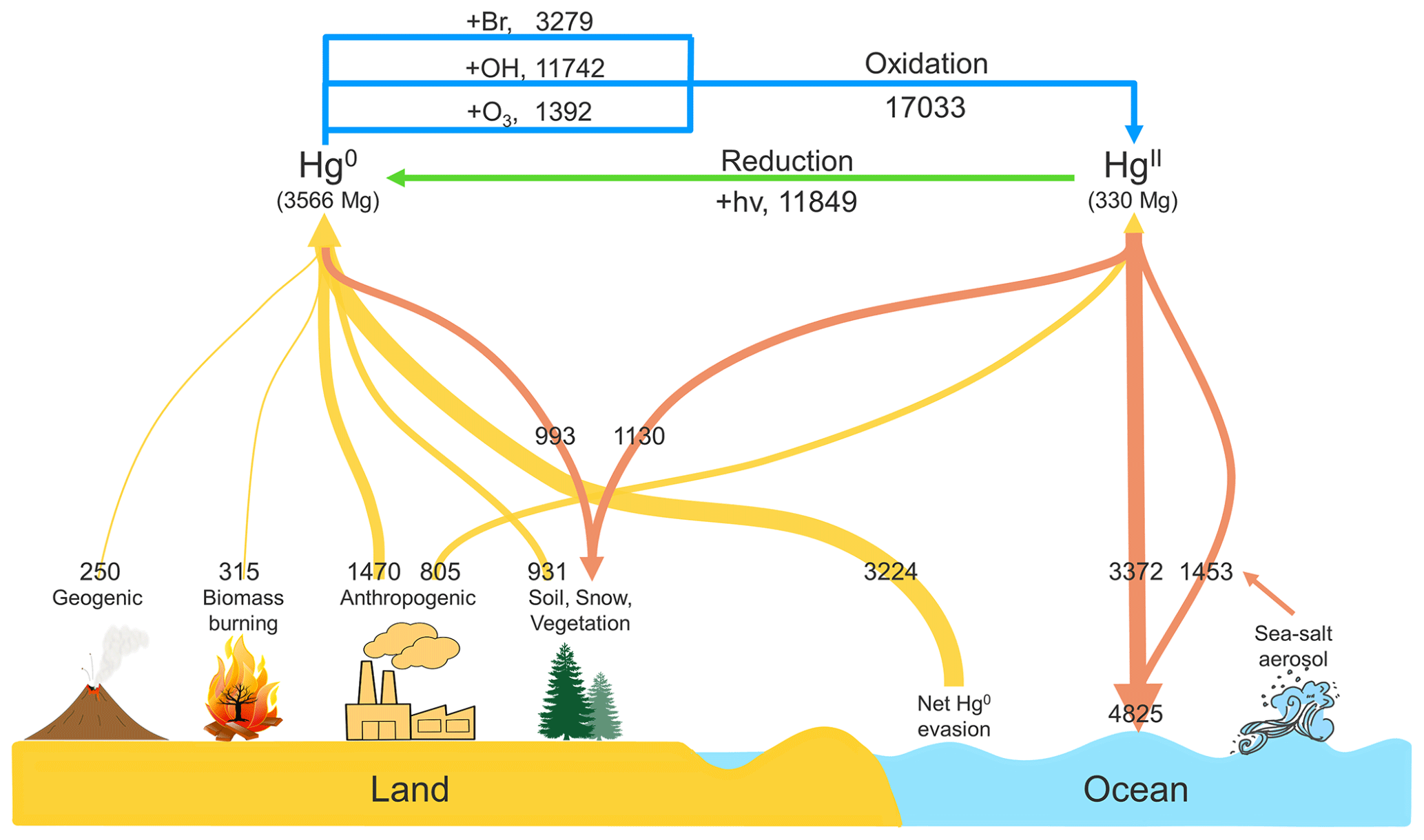
Figure 1Global budget of atmospheric mercury in CAM6-Chem/Hg. Only the reaction rates of three major oxidants are shown. Fluxes in Mg a−1. The thickness of the arrows represents the relative contribution.
2.2 Mercury emission
Both anthropogenic and natural Hg emissions are included in the CAM6-Chem/Hg model (Fig. 1). The anthropogenic emissions used in this study are consistent with Horowitz et al. (2017). They are based on an improved 2010 global inventory developed by Zhang et al. (2016), which considered the release of Hg from commercial products and emission controls on coal combustion. The total anthropogenic emissions are 2275 Mg a−1, of which 1470 and 805 Mg a−1 are for Hg0 and HgII respectively.
The natural emissions and re-emissions from previously deposited legacy emissions are derived from the average of a 5-year simulation in GEOS-Chem v11 (Horowitz et al., 2017), including geogenic, biomass burning, soil, ocean, snow, and vegetation emissions. The simulation is conducted at 4∘ × 5∘ horizontal resolution and then mapped to 0.9∘ × 1.25∘ for CAM6-Chem. Since the ocean model (POP2) of the CESM2 used in CAM6-Chem/Hg is a data component, the exchange process of Hg0 between atmosphere and ocean is replaced with a net emission from ocean. This net ocean emission is about 3200 Mg a−1 and falls in the range of 2840 to 3710 Mg a−1 indicated by recent online air–sea coupling model research (Zhang et al., 2019). The natural emission from land is about 1500 Mg a−1, which is similar to the previous estimation used in GEOS-Chem (Horowitz et al., 2017). Future work will have more explicit natural/legacy emissions and improve the calculation of the fluxes between different spheres by introducing Hg simulations into other models (e.g., CLM5 and POP2).
2.3 Mercury chemistry
Possible oxidants of Hg0 include , Br, or other halogens. Although the oxidation of Hg0 by OH has been controversial, mainly due to the rapid thermal decomposition of its intermediate product HgOHI (Goodsite et al., 2004; Calvert and Lindberg, 2005), a recent study recalculated the HO–Hg bond energy and found that the OH-initiated oxidation of Hg plays an important role in polluted regions (Dibble et al., 2020). It is noted that neither oxidation by Br nor alone in the model could reproduce the global or regional observations (Wang et al., 2014; Weiss-Penzias et al., 2015; Ye et al., 2016; Bieser et al., 2017; Gencarelli et al., 2017; Travnikov et al., 2017). Therefore, we adopt multiple pathways including both Br and as the oxidants of Hg0. The Hg0 oxidation by Br atoms is considered as a two-step process with rates following Horowitz et al. (2017). The oxidation by adopts the reaction rates used in Lei et al. (2013), except that the product is assumed to be HgII in our simulation. Different from the HgII partitioning used in the previous studies (Holmes et al., 2010; Lei et al., 2013), we adopt an empirical relationship introduced by Amos et al. (2012) to deal with the gas-particle partitioning of HgII, considering the influence of fine particulate matter (PM2.5) and temperature. Several possible HgII reduction pathways have been proposed (Si and Ariya, 2018), and we adopt the aqueous photoreduction of HgII-organic complexes used in Horowitz et al. (2017). The best match with the available total gaseous mercury (TGM) surface observations and Hg wet deposition fluxes can be obtained by adjusting the photoreduction rate coefficient (Horowitz et al., 2017; Shah et al., 2021).
The representation of the main oxidants (e.g., O3 and OH) of Hg0 has been greatly improved and is more comprehensive in the CAM6-Chem compared with its predecessors CESM or CCSM. The simulated tropospheric O3 also agrees better with ozonesonde observations worldwide (Lamarque et al., 2012; Emmons et al., 2020). The CAM6-Chem contains the sources of Br from the photodecomposition of organobromines (CHBr3, CH2Br2, CH3Br), the homogeneous and heterogeneous bromine chemistry reactions, as well as the chlorine chemistry (for more details see TS1 mechanism in Emmons et al., 2020). Our model takes advantage of these improvements and couples the atmospheric chemistry of Hg with its oxidants for the first time.
2.4 Mercury deposition
The removal of Hg from the atmosphere includes wet and dry deposition processes. Considering the differences in physical and chemical properties of atmospheric Hg species, different approaches are used to simulate deposition in CAM6-Chem/Hg. For Hg0 and Hg2, we adopt the default schemes used in CAM6-Chem for the dry and wet deposition of gas-phase compounds (see Sect. 2.1). The dry deposition rates of Hg0 and Hg2 are calculated online in the CLM5 model based on the land use types. The wet removal of Hg2 includes both in-cloud and below-cloud processes. In addition, the uptake and deposition of Hg2 by sea-salt aerosol are parameterized following Holmes et al. (2010) as a first-order loss rate in the marine boundary layer (MBL). For HgP, its treatment for dry and wet deposition is the same as other aerosol species in CAM6-Chem.
2.5 Model run
In this work, a 4-year (2010–2013) free-running simulation is conducted in CAM6-Chem/Hg, with specified sea surface temperature. We use the initial year (i.e., 2010) as a spin-up to minimize the impact of initial conditions and the average of the following 3 years (i.e., 2011–2013, with abundant observations during the past decades) for analysis (unless explicitly stated). The model's initial state is taken from the output of the GEOS-Chem model (Horowitz et al., 2017) and linearly interpolated to the CAM6-Chem model grid.
3.1 Global atmospheric Hg budget
Figure 1 shows the global budget of Hg derived from our CAM6-Chem/Hg simulation, including the reactions with three major oxidants (Br, OH, and O3) and the photoreduction rates. The oxidation with OH radicals is an important pathway when considering the proportion of oxidation rates, consistent with previous studies (Selin et al., 2007; Shah et al., 2021). And the dominant oxidation pathways differ across regions, which shows peaks in the mid-to-low latitude terrestrial regions for OH, while the oxidation by Br is stronger in the marine regions (Fig. S1 in the Supplement). This spatial distribution of different oxidation pathways is also consistent with the recent isotope data (AuYang et al., 2022). The reservoir of global atmospheric Hg is 3896 Mg, of which Hg0 and HgII are 3566 and 330 Mg, respectively (for HgII, 122 and 208 Mg in the gaseous and particulate phases, respectively). The global total Hg emissions from all sources are about 7000 Mg a−1; two-thirds of these are natural/legacy emissions. In this study, the rapid re-emission of deposited Hg0 is included in the land emission and the Hg0 dry deposition to the ocean is replaced with the net Hg0 evasion. The lifetime of total gaseous mercury (TGM = Hg0+Hg2) against deposition is 5.3 months in our simulation, which is in accordance with the estimation in the GEOS-Chem model (Holmes et al., 2010; Horowitz et al., 2017).
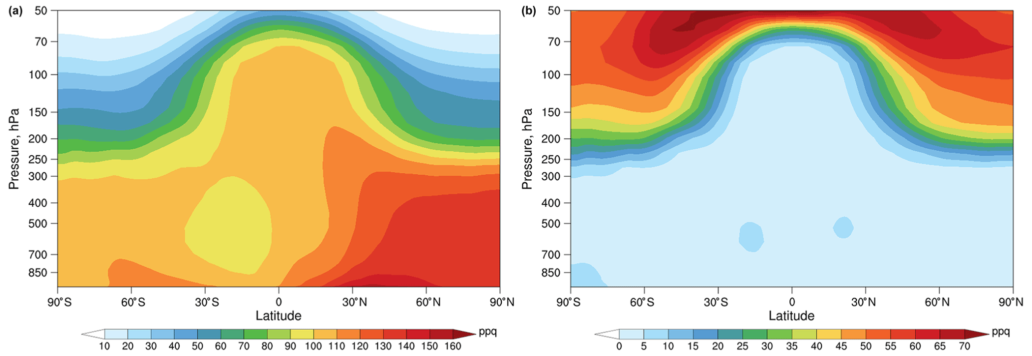
Figure 2Annual (2011–2013) zonal mean concentrations of Hg0 (a) and HgII (b) in CAM6-Chem/Hg.
The modeled vertical distributions of the annual zonal mean mixing ratios of Hg0 and HgII are shown in Fig. 2. Hg0 is the dominant chemical species in the troposphere and is higher in the Northern Hemisphere (NH) than in the Southern Hemisphere (SH) due to anthropogenic emissions. The simulated Hg0 concentration is relatively uniform in the troposphere but decreases rapidly around the tropopause. The simulated HgII increases with altitude and is more abundant in the stratosphere. These vertical distributions of Hg0 and HgII are consistent with previous model studies (Holmes et al., 2010; Horowitz et al., 2017) and available aircraft measurements (Talbot et al., 2008; Lyman and Jaffe, 2012; Slemr et al., 2018).
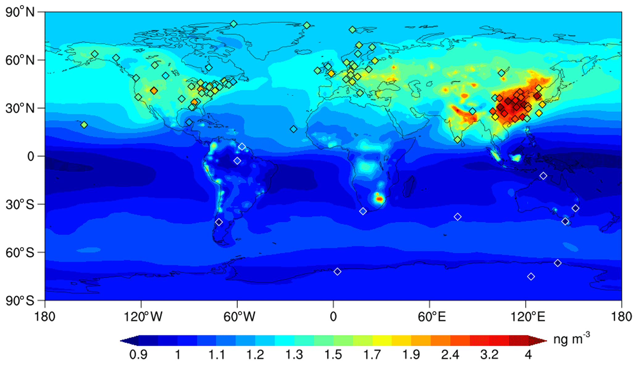
Figure 3Global distribution of surface total gaseous mercury (TGM) concentrations. Model results (background) are annual average of 2011–2013. Ground-based observations (rhombuses) are for 2009–2015 except for some observations in eastern Asia (see Table S1 in the Supplement for detailed description). The rhombuses with white frames are concentrations below 1.2 ng m−3. Note that the scale of the color bar is non-uniform.
3.2 Atmospheric Hg concentrations
The global distribution of surface TGM concentrations is shown in Fig. 3 with our simulation compared to the available ground-based observations during 2009–2015 (except for some observations in eastern Asia that are out of this time range; see Table S1 in the Supplement for detailed description). In general, the mean and standard deviation at the 92 land sites are 1.78±1.02 ng m−3 for the model, agreeing well with the observations (1.75±0.86 ng m−3). Our model also reproduces the global distribution of TGM well with high correlation coefficients (r=0.83).

Figure 4The latitudinal variation of surface TGM concentrations. The red line and shaded areas are the modeled means and standard deviations of 2011–2013, respectively. The two black dashed lines represent the locations of the Tropic of Capricorn and Cancer. The observations (rhombuses) at land sites only include part of the values (<2 ng m−3) as shown in Fig. 3.
The modeled global mean of surface TGM concentrations is 1.14 ng m−3 with a higher value in the NH (1.27 ng m−3) than in the SH (1.02 ng m−3), indicating a significant cross-hemisphere gradient (Fig. 4). Overall, the CAM6-Chem/Hg can capture the peak values in the northern mid-latitudes and the lower ones in the SH. A gradual increasing trend from south to north is in line with the limited land-based observations in the tropics (Fig. 4). This simulated interhemispheric gradient of TGM also agrees with observational studies in the marine boundary layer (Soerensen et al., 2010a; Sprovieri et al., 2010, 2016) and previous modeling studies (Lamborg et al., 2002; Selin et al., 2007; Holmes et al., 2010; Travnikov et al., 2017). We attribute this interhemispheric gradient to the large disparity in Hg emissions in the two hemispheres. In CAM6-Chem/Hg, the total anthropogenic emissions in the NH are about 7-fold higher than that in the SH and are 1.5-fold for total emissions (natural emissions in the SH partially offset the large difference in emissions).
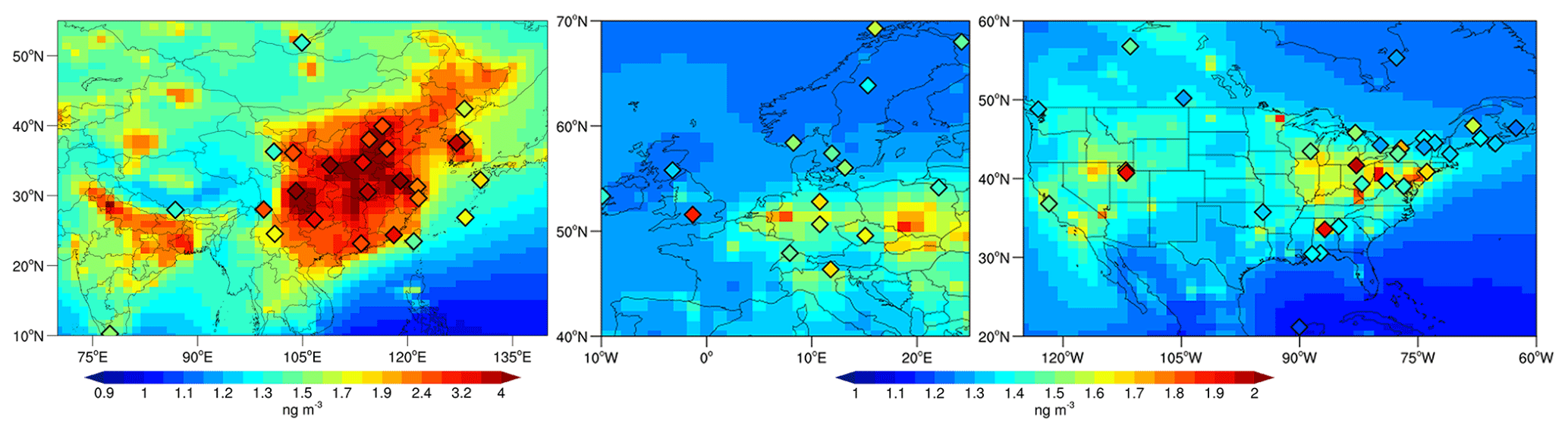
Figure 5Regional distribution of surface TGM concentrations in eastern Asia, western Europe, and North America. Ground-based observations (rhombuses) are the same as Fig. 3. Note that two different color bars are used to depict regional variations.
The standard deviations of TGM concentrations are large for both model and observations, indicating large regional variability, especially between polluted and background areas. Figure 5 shows the modeled results in three regions with elevated TGM concentrations: eastern Asia (10–55∘ N, 70–140∘ E), western Europe (40–70∘ N, 10∘ W–25∘ E) and North America (20–60∘ N, 60–125∘ W). Eastern Asia is one of the regions most contaminated by Hg in the world (Sprovieri et al., 2016). The observed mean TGM concentrations at the available 26 land sites are 2.69±1.16 ng m−3. The high standard deviation reflects the large spatial variability within eastern Asia. Eight sites are higher than 3 ng m−3 and three are above 4 ng m−3, including Xi'an (5.66 ng m−3, Xu et al., 2017), Nanjing (4.98 ng m−3, our own data), and Chengdu (4.56 ng m−3, Fu et al., 2021) in China. These high-concentration sites are usually located in urban or suburban regions which are close to the large anthropogenic emission sources. Our model agrees with the observations quite well (2.97±1.28 ng m−3) with a spatial correlation coefficient (r) of 0.67. The observed TGM concentrations in western Europe are lower (1.53±0.15 ng m−3, n=15 sites) than in eastern Asia. We find the model (1.31±0.09 ng m−3) slightly underestimates the observations (r=0.22), but the model simulates high values in central and eastern regions, which is consistent with the observations and high emissions in these areas (Pacyna et al., 2001, 2006). In North America, the observed TGM concentrations are 1.47±0.20 ng m−3 (n=30), similar to the TGM level in western Europe. The model (1.43±0.15 ng m−3) also agrees well with the observations (r=0.57). The modeled TGM shows relatively higher concentrations in the eastern and western United States but relatively uniform and low in the central area, consistent with the spatial distribution of anthropogenic emissions of Hg (the scatter diagrams of comparison between simulation and observations are shown in Fig. S2 in the Supplement). The agreement between observations and model results in these areas implies that our model performs well in polluted regions. In addition, the modeled TGM concentrations in north-eastern India are also high (left panel in Fig. 5), calling for more observations to constrain the model.
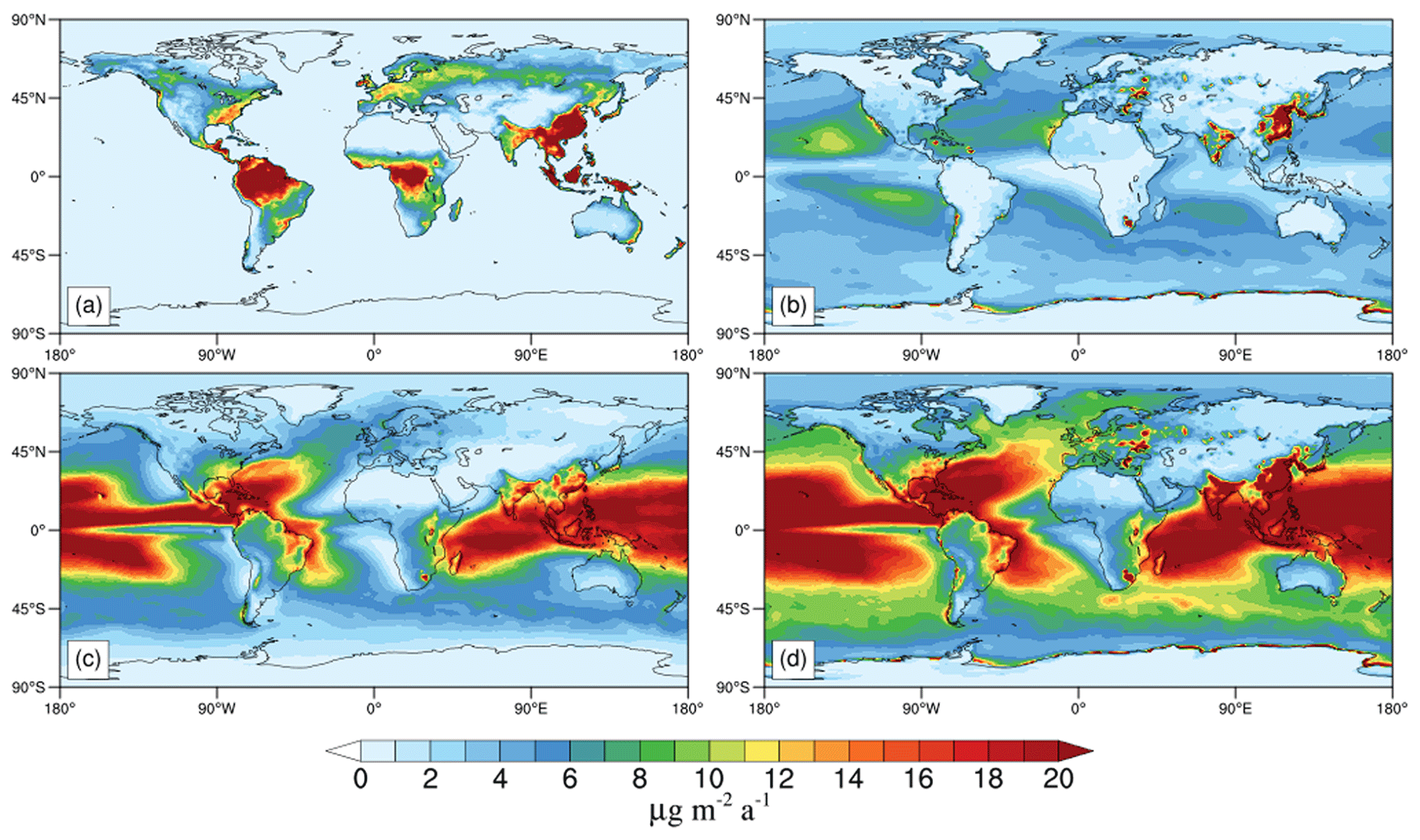
Figure 6Global distribution of annual mean Hg deposition fluxes during 2011–2013 in CAM6-Chem/Hg: (a) Hg0 dry deposition, (b) HgII dry deposition (including sea-salt uptake), (c) HgII wet deposition, and (d) HgII total deposition.
3.3 Atmospheric Hg depositions
Figure 6a shows the distribution of Hg0 dry deposition worldwide (the deposition to the ocean is considered as a net re-emission from the ocean, i.e., gross evasion minus deposition). The annual global dry deposition flux of Hg0 over land is 993 Mg a−1, and more than half is distributed in the tropics (23.26∘ S–23.26∘ N). This Hg0 deposition flux is slightly smaller than previous GEOS-Chem models (1200–1600 Mg a−1, Selin et al., 2008; Holmes et al., 2010; Horowitz et al., 2017) due to different parameter settings (e.g., grid resolution, land types, and meteorological data) between these models. The dry deposition flux is based on the dry deposition velocity and the local Hg0 concentration. Fluxes are higher over northern South America, central Africa, southeastern Asia, and eastern Asia. The high flux in eastern Asia is driven by the high Hg0 concentration, whereas the Hg0 concentrations over the other three regions are relatively low (see Fig. 3). As described in Sect. 2.1, the dry deposition velocities are affected by the leaf area index (LAI), which depends on seasons and land use types, as modeled by the CLM5. The major land use type of these three regions is tropical rainforests, which leads to a high dry deposition velocity and subsequently high dry deposition flux.
Figure 6b and c show the global distribution of dry and wet annual deposition flux of HgII respectively (the uptake of HgII by sea-salt aerosol is included in dry deposition). The total HgII deposition is 5954 Mg a−1 (Fig. 6d), of which the proportions of dry and wet deposition are 9 % and 67 % respectively, compared to 16 % and 61 % in Holmes et al. (2010). The rest is the uptake by sea-salt aerosol (1453 Mg a−1), which has been proved to be an important sink for HgII in the MBL in previous research (Holmes et al., 2009, 2010; Malcolm et al., 2009). HgII deposited to the ocean accounts for 81 % of the global total deposition, while the land takes the remaining 19 %. These proportions are consistent with Horowitz et al. (2017), but our model shows a higher flux in low latitudes. The global total HgII deposition to tropical oceans (30∘ S–30∘ N) in our simulation is 3328 Mg a−1, higher than 2800 Mg a−1 in Horowitz et al. (2017). This is partly due to the addition of oxidation mechanisms. The OH concentration is the greatest at low latitudes in the lower to the middle troposphere (Crutzen and Zimmermann, 1991; Spivakovsky et al., 2000; Lelieveld et al., 2016), which causes more Hg0 oxidation to HgII, and the frequent deep convective precipitation promotes the wet removal of HgII in the tropics. Another reason for the difference could be the different Br concentrations. As the debromination of sea salt aerosol is not included in CAM6-Chem, the model may underestimate the concentrations of Br in the MBL. Indeed, the mean tropospheric Br and BrO concentrations are 0.03 and 0.13 ppt respectively, which are lower than 0.08 and 0.48 ppt in Schmidt et al. (2016) but are more consistent with 0.03 and 0.19 ppt simulated by Wang et al. (2021). The vertical distributions of zonal mean Br and BrO are shown in Fig. S3. The total HgII deposition to the ocean is about 1600 Mg a−1 higher than the net ocean emission in our simulation, which means that globally the ocean is a net atmospheric Hg sink (Soerensen et al., 2010b; Horowitz et al., 2017), especially in tropical oceans with intensive precipitation.

Figure 7Comparison between modeled (background) and observed (circles) annual HgII wet deposition fluxes over North America for 2011–2013. Annual observations are derived from the Mercury Deposition Network (MDN, National Atmospheric Deposition Program, http://nadp.slh.wisc.edu/MDN/, last access: 19 January 2022) during 2009–2015.
We also compare the modeled HgII wet deposition fluxes against observations over three regions in the NH: North America, eastern Asia, and western Europe. In North America, the model simulates a spatial distribution pattern that gradually increases from northwest to southeast in CONUS that is consistent well with the observations (r=0.80, n=147) (Fig. 7). Previous models using Br as the sole oxidant (e.g., GEOS-Chem) failed to capture the maximum or underestimated the magnitude of HgII wet deposition along the coast of the Gulf of Mexico (Holmes et al., 2010; Amos et al., 2012; Horowitz et al., 2017). Our simulation with multiple oxidants agrees better with the observed maximum deposition fluxes (15–20 ), especially in the Florida Peninsula. The scatter plot of observed and modeled annual mean HgII wet deposition flux is shown in Fig. S4. In a model comparison study, Travnikov et al. (2017) found that the oxidation mechanisms showed a better agreement between modeled and observed wet deposition than the Br oxidation mechanism, consistent with our study.
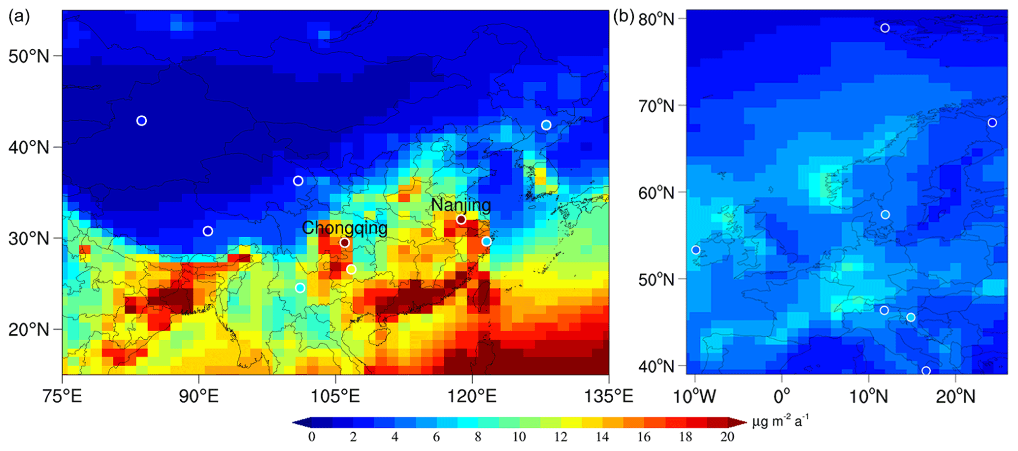
Figure 8Same as Fig. 7, but for eastern Asia (a) and western Europe (b). The observations (circles) are derived from recent studies by Fu et al. (2015, 2016) and Sprovieri et al. (2017), respectively. For eastern Asia, only data with >9 months of data during 2009–2015 are included in the observations for comparison. For western Europe, the sites with sampling days greater than 60 % in a year are taken as available observations.
Figure 8 shows the HgII wet deposition over eastern Asia and western Europe, where the available observations are more limited (n=9 and 7, respectively). In eastern Asia, the spatial distribution of HgII wet deposition shows an increasing trend from inland northwest to coastal southeast, reflecting the pattern in anthropogenic emissions. The model captures the spatial distribution quite well (r=0.53). Similar to North America, the model also simulates the maximum deposition flux over southeastern China, probably due to the frequent convective precipitation there. More observations in this region are indeed needed to confirm this prediction. Compared with the simulation by Horowitz et al. (2017), our model agrees better with limited observations in Chongqing and Nanjing, likely owing to the higher horizontal resolution of our model that improves the representation of emissions and precipitation (Zhang et al., 2012).
Compared to the above two regions, our simulation shows much smaller deposition flux and less spatial variability over western Europe. This pattern in general agrees with the observations (r=0.74), reflecting the fact that the wet deposition flux is much higher at low latitudes than high latitudes (Fig. 6c). The wet deposition flux is relatively high in the central regions (over Germany, United Kingdom, and Norway), where the Hg emissions are higher than other western European regions (Pacyna et al., 2006; Ballabio et al., 2021). Apart from the impact of emissions, our model shows a high correlation between precipitation and wet deposition fluxes (r=0.72) in western Europe, indicating a strong influence of precipitation on Hg wet deposition flux over this region.
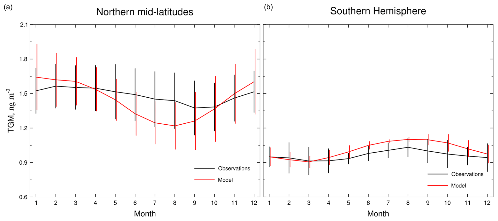
Figure 9Seasonal variations of surface TGM concentrations in northern mid-latitudes (a) and the Southern Hemisphere (b). Observations are the average of the available monthly data from the ground-based sites in Fig. 3, indicated by the black line. The red line represents the results simulated by CAM6-Chem/Hg model. Error bar depicts the standard deviation of TGM concentrations.
Figure 9 compares modeled and observed seasonal variations of TGM concentrations at ground-based sites in northern mid-latitudes (30–60∘ N, n=43) and the SH (n=5). In northern mid-latitudes, the observed TGM reaches the maximum in February and is the lowest in September. In the SH, the observed TGM reaches the maximum in August and the minimum in March. In both hemispheres, the simulated results generally reproduce the observed seasonal variations. Notably, the modeled amplitude of seasonal variability is greater in northern mid-latitudes than in the SH. Such a pattern has also been reported by several modeling studies (Selin et al., 2007; Holmes et al., 2010; De Simone et al., 2014; Horowitz et al., 2017) and is mainly attributed to four factors: anthropogenic and natural emissions, meteorological factors, Hg0 oxidation rates, and HgII deposition (Temme et al., 2007; Ebinghaus et al., 2011; Fu et al., 2015; Weigelt et al., 2015; Sprovieri et al., 2016). However, the role of Hg0 uptake by vegetation is emphasized in a recent work (Jiskra et al., 2018), which shows a considerable contribution to the seasonal variation of atmospheric Hg0 distribution.

Figure 10Seasonal variations of atmospheric Hg in (a) Northern Hemisphere, (b) Northern Hemisphere land areas only, (c) Northern Hemisphere ocean areas only, (d) Southern Hemisphere, (e) Southern Hemisphere land areas only, and (f) Southern Hemisphere ocean areas only. The bars represent the anomaly of different processes: deep blue for Hg0 dry deposition, cyan for HgII dry deposition, jacinth for HgII wet deposition, and orange for Hg0 natural/legacy emission. The first three are reversed for their signs as they are sinks of Hg. The anomaly of the difference between the source and the sink is shown as the red dashed line with circles, and the solid black line with circles is the anomaly of the total mass of atmospheric Hg. The solid green line represents the surface Hg concentrations.
We use the CAM6-Chem/Hg model to quantify the relative contribution of different factors to the seasonal variations of atmospheric Hg on a global scale. Since the anthropogenic emissions of Hg remain constant throughout the years in our simulation, we do not take this factor into account. Figure 10 shows the contributions of a variety of processes (dry and wet deposition fluxes for Hg0 and HgII, as well as Hg0 natural and legacy emissions) over land/ocean in the NH and SH for the year 2013. In the NH, Hg0 dry deposition and HgII dry/wet deposition have negative anomalies during November–April (bars and the red dashed line), leading to a continuous increase of atmospheric Hg levels (black line). Overall, HgII dry/wet deposition (cyan and jacinth color bars, respectively) contributes the most (53 %) to this increase, followed by Hg0 dry deposition (deep blue color bars, 28 %) and the natural/legacy emissions (orange color bars, 19 %). During May–October, the removal processes of Hg from the atmosphere are higher than the annual average, which has caused a decrease in atmospheric Hg levels. Similarly, HgII dry/wet depositions are also the leading driving factor for this trend.
We find the changes of atmospheric Hg levels (black line) do not agree with the net source/sink terms for some months (e.g., October) (Fig. 10a, red dashed line), likely due to the mixing time required for the source–sink processes to influence the hemispheric Hg pool. We thus split the global atmosphere into over land (Fig. 10b) and over ocean (Fig. 10c), respectively. The result over land is similar to that in the NH, but without significant lag between the net source/sink terms and the atmospheric Hg levels. We find that the contribution of Hg0 dry deposition (40 %) to the seasonal variations outweighs that of HgII wet depositions (32 %) throughout the year, confirming previous thoughts (Wright et al., 2016; Jiskra et al., 2018; Obrist et al., 2021). However, we argue that the importance of HgII total depositions also plays an important role, contributing 40 % of the seasonality. The seasonal pattern of net source/sink terms over ocean (Fig. 10c) is smoother compared to that on the land. The seasonal cycle is largely driven by the ocean re-emissions and HgII wet depositions.
In the SH, we find the influence of Hg0 dry deposition is much smaller than that of the NH, due to its much smaller land mass. HgII depositions and Hg0 natural/legacy emissions are the driving factors for the seasonal patterns of atmospheric Hg (Fig. 10d). Notably, the amplitude of variation in atmospheric Hg level and net source/sink terms in the SH exceeds that of the NH. HgII dry/wet deposition and Hg0 dry deposition show negative anomalies during April–September, resulting in a sustained increase in atmospheric Hg levels. Slightly different from the NH, HgII dry/wet deposition contributes the most (66 %) to this increase, followed by the natural/legacy emissions (28 %) and Hg0 dry deposition (6 %). Not surprisingly, we find a much smaller seasonal amplitude for atmospheric Hg over SH land (Fig. 10e) than NH land (Fig. 10b) as a result of the lack of contribution from Hg0 dry depositions. This result is supported by the observations in the Global Atmosphere Watch station at Cape Point, which shows a similar seasonal variation with our model (Sprovieri et al., 2016). The agreement between our model-derived net source/sink terms and atmospheric Hg levels is also the best (discrepancy Mg) among the land/ocean regions in the two hemispheres. Over the ocean, we find the HgII wet deposition is the major driver for the seasonality (52 %), followed by HgII dry deposition (25 %) and seawater Hg0 evasion (23 %).
In conclusion, although the seasonal variations of atmospheric Hg in the NH and SH are similar, the relative contribution of different processes to the variations is different. It is a combination of different source and sink terms on a hemispheric scale, while there may be a dominant driving factor on a regional scale.
The atmosphere is one of the most active parts of the global mercury cycle, as well as an important component for the mercury exchange between different components of the Earth system. Here we develop a new online global 3-D atmospheric mercury model (CAM6-Chem/Hg) and implement a chemical mechanism with multiple oxidation pathways of Hg. We use the online meteorological fields and built-in chemical species to drive the transport and physiochemical processes of Hg in the atmosphere. This online method reduces the uncertainties caused by the interpolation of external meteorological data and chemical species.
Two main oxidation pathways, Hg + Br and Hg + , are used together in the chemical mechanism. In our simulation, the lifetime of total gaseous mercury (TGM) against deposition is about 5.3 months, which is consistent with the observational constraints. The CAM6-Chem/Hg model also reproduced the ground-based observations and the interhemispheric gradient of TGM concentrations well. The global nominal 1∘ horizontal resolution used in CAM6-Chem/Hg can capture the distribution characteristics of TGM concentrations better on regional scales, especially in some high anthropogenic emission regions (e.g., eastern Asia). In particular, the CAM6-Chem/Hg calculates the Hg0 dry deposition velocity online through coupling with the land component (i.e., CLM5) in CESM2, which can take the land-use types and seasonal variation into a good account. Compared with Br as the sole oxidant, adding as oxidants leads to a broader range and higher flux of HgII wet deposition in low latitudes. The simulated HgII wet deposition flux is consistent with the available observations and captures the magnitude of the maximum value in the southeastern United States. Shah et al. (2021) presented a new chemical mechanism for atmospheric Hg in GEOS-Chem, and the CAM6-Chem/Hg presented here provides a convenient platform to integrate the updated Hg chemistry with online meteorology and atmospheric chemistry.
The CAM6-Chem/Hg reproduces the observed seasonal variations of TGM concentrations in northern mid-latitudes and the Southern Hemisphere, which show a trend of decrease in spring and summer and increase in autumn and winter. We use the model to quantify the processes affecting the seasonality of atmospheric Hg from the relationship between sources and sinks. On the hemispherical scale, the seasonal changes of deposition have an important influence on atmospheric Hg, followed by natural and re-emission sources. In the land region of the Northern Hemisphere, the contribution of Hg0 dry deposition to seasonal variations of Hg outweighs that of HgII wet deposition. The seasonal variations of atmospheric Hg are the result of multiple processes and have obvious regional characteristics. Research on Hg0 dry deposition will improve our understanding of the seasonal cycle of atmospheric Hg.
The CESM2 model code is available at https://www.cesm.ucar.edu/models/cesm2/release_download.html (last access: 19 January 2022). The code used for implementing mercury into CAM6-Chem (CAM6-Chem/Hg v1.0) in this study is permanently archived on Zenodo at https://doi.org/10.5281/zenodo.5877214 (Zhang and Zhang, 2022).
The data supporting the findings of this study are available within the article and its Supplement.
The supplement related to this article is available online at: https://doi.org/10.5194/gmd-15-3587-2022-supplement.
YZ and PZ conceived the idea and designed the model experiments. PZ and YZ modified the code of the model. PZ performed the simulations, conducted the analysis, and wrote the paper. YZ and PZ edited the paper.
The contact author has declared that neither they nor their co-author has any competing interests.
Publisher's note: Copernicus Publications remains neutral with regard to jurisdictional claims in published maps and institutional affiliations.
The CESM project is supported primarily by the National Science Foundation (NSF). We thank all the scientists, software engineers, and administrators who contributed to the development of CESM2. We would like to acknowledge and thank all the operators who collected the observations used in this work.
This research has been supported by the National Key Research and Development Program of China (grant no. 2019YFA0606803), the National Natural Science Foundation of China (grant no. 71974092), and the Fundamental Research Funds for the Central Universities (grant no. 0207-14380168), Frontiers Science Center for Critical Earth Material Cycling.
This paper was edited by Havala Pye and reviewed by two anonymous referees.
Amos, H. M., Jacob, D. J., Holmes, C. D., Fisher, J. A., Wang, Q., Yantosca, R. M., Corbitt, E. S., Galarneau, E., Rutter, A. P., Gustin, M. S., Steffen, A., Schauer, J. J., Graydon, J. A., Louis, V. L. St., Talbot, R. W., Edgerton, E. S., Zhang, Y., and Sunderland, E. M.: Gas-particle partitioning of atmospheric Hg(II) and its effect on global mercury deposition, Atmos. Chem. Phys., 12, 591–603, https://doi.org/10.5194/acp-12-591-2012, 2012.
AuYang, D., Chen, J., Zheng, W., Zhang, Y., Shi, G., Sonke, J. E., Cartigny, P., Cai, H., Yuan, W., Liu, L., Gai, P., and Liu, C.: South-hemispheric marine aerosol Hg and S isotope compositions reveal different oxidation pathways, National Science Open, 1, 20220014, https://doi.org/10.1360/nso/20220014, 2022.
Baklanov, A., Schlünzen, K., Suppan, P., Baldasano, J., Brunner, D., Aksoyoglu, S., Carmichael, G., Douros, J., Flemming, J., Forkel, R., Galmarini, S., Gauss, M., Grell, G., Hirtl, M., Joffre, S., Jorba, O., Kaas, E., Kaasik, M., Kallos, G., Kong, X., Korsholm, U., Kurganskiy, A., Kushta, J., Lohmann, U., Mahura, A., Manders-Groot, A., Maurizi, A., Moussiopoulos, N., Rao, S. T., Savage, N., Seigneur, C., Sokhi, R. S., Solazzo, E., Solomos, S., Sørensen, B., Tsegas, G., Vignati, E., Vogel, B., and Zhang, Y.: Online coupled regional meteorology chemistry models in Europe: current status and prospects, Atmos. Chem. Phys., 14, 317–398, https://doi.org/10.5194/acp-14-317-2014, 2014.
Ballabio, C., Jiskra, M., Osterwalder, S., Borrelli, P., Montanarella, L., and Panagos, P.: A spatial assessment of mercury content in the European Union topsoil, Sci. Total Environ., 769, 144755, https://doi.org/10.1016/j.scitotenv.2020.144755, 2021.
Bieser, J., Slemr, F., Ambrose, J., Brenninkmeijer, C., Brooks, S., Dastoor, A., DeSimone, F., Ebinghaus, R., Gencarelli, C. N., Geyer, B., Gratz, L. E., Hedgecock, I. M., Jaffe, D., Kelley, P., Lin, C.-J., Jaegle, L., Matthias, V., Ryjkov, A., Selin, N. E., Song, S., Travnikov, O., Weigelt, A., Luke, W., Ren, X., Zahn, A., Yang, X., Zhu, Y., and Pirrone, N.: Multi-model study of mercury dispersion in the atmosphere: vertical and interhemispheric distribution of mercury species, Atmos. Chem. Phys., 17, 6925–6955, https://doi.org/10.5194/acp-17-6925-2017, 2017.
Calvert, J. G. and Lindberg, S. E.: Mechanisms of mercury removal by O3 and OH in the atmosphere, Atmos. Environ., 39, 3355–3367, https://doi.org/10.1016/j.atmosenv.2005.01.055, 2005.
Crutzen, P. J. and Zimmermann, P. H.: The changing photochemistry of the troposphere, Tellus A, 43, 136–151, https://doi.org/10.1034/j.1600-0870.1991.00012.x, 1991.
Danabasoglu, G., Lamarque, J. F., Bacmeister, J., Bailey, D. A., DuVivier, A. K., Edwards, J., Emmons, L. K., Fasullo, J., Garcia, R., Gettelman, A., Hannay, C., Holland, M. M., Large, W. G., Lauritzen, P. H., Lawrence, D. M., Lenaerts, J. T. M., Lindsay, K., Lipscomb, W. H., Mills, M. J., Neale, R., Oleson, K. W., Otto Bliesner, B., Phillips, A. S., Sacks, W., Tilmes, S., Kampenhout, L., Vertenstein, M., Bertini, A., Dennis, J., Deser, C., Fischer, C., Fox Kemper, B., Kay, J. E., Kinnison, D., Kushner, P. J., Larson, V. E., Long, M. C., Mickelson, S., Moore, J. K., Nienhouse, E., Polvani, L., Rasch, P. J., and Strand, W. G.: The Community Earth System Model Version 2 (CESM2), J. Adv. Model. Earth Sy., 12, e2019MS001916, https://doi.org/10.1029/2019MS001916, 2020.
De Simone, F., Gencarelli, C. N., Hedgecock, I. M., and Pirrone, N.: Global atmospheric cycle of mercury: a model study on the impact of oxidation mechanisms, Environ. Sci. Pollut. R., 21, 4110–4123, https://doi.org/10.1007/s11356-013-2451-x, 2014.
Dibble, T. S., Tetu, H. L., Jiao, Y., Thackray, C. P., and Jacob, D. J.: Modeling the OH-Initiated Oxidation of Mercury in the Global Atmosphere without Violating Physical Laws, J. Phys. Chem. A, 124, 444–453, https://doi.org/10.1021/acs.jpca.9b10121, 2020.
Driscoll, C. T., Mason, R. P., Chan, H. M., Jacob, D. J., and Pirrone, N.: Mercury as a Global Pollutant: Sources, Pathways, and Effects, Environ. Sci. Technol., 47, 4967–4983, https://doi.org/10.1021/es305071v, 2013.
Durnford, D., Dastoor, A., Ryzhkov, A., Poissant, L., Pilote, M., and Figueras-Nieto, D.: How relevant is the deposition of mercury onto snowpacks? – Part 2: A modeling study, Atmos. Chem. Phys., 12, 9251–9274, https://doi.org/10.5194/acp-12-9251-2012, 2012.
Ebinghaus, R., Jennings, S. G., Kock, H. H., Derwent, R. G., Manning, A. J., and Spain, T. G.: Decreasing trends in total gaseous mercury observations in baseline air at Mace Head, Ireland from 1996 to 2009, Atmos. Environ., 45, 3475–3480, https://doi.org/10.1016/j.atmosenv.2011.01.033, 2011.
El-Harbawi, M.: Air quality modelling, simulation, and computational methods: a review, Environ. Rev., 21, 149–179, https://doi.org/10.1139/er-2012-0056, 2013.
Emmons, L. K., Schwantes, R. H., Orlando, J. J., Tyndall, G., Kinnison, D., Lamarque, J. F., Marsh, D., Mills, M. J., Tilmes, S., Bardeen, C., Buchholz, R. R., Conley, A., Gettelman, A., Garcia, R., Simpson, I., Blake, D. R., Meinardi, S., and Pétron, G.: The Chemistry Mechanism in the Community Earth System Model Version 2 (CESM2), J. Adv. Model. Earth Sy., 12, e2019MS001882, https://doi.org/10.1029/2019MS001882, 2020.
Fernandez, R. P., Carmona Balea, A., Cuevas, C. A., Barrera, J. A., Kinnison, D. E., Lamarque, J. F., Blaszczak Boxe, C., Kim, K., Choi, W., Hay, T., Blechschmidt, A. M., Schönhardt, A., Burrows, J. P., and Saiz Lopez, A.: Modeling the Sources and Chemistry of Polar Tropospheric Halogens (Cl, Br, and I) Using the CAM-Chem Global Chemistry-Climate Model, J. Adv. Model. Earth Sy., 11, 2259–2289, https://doi.org/10.1029/2019MS001655, 2019.
Fu, X., Yang, X., Lang, X., Zhou, J., Zhang, H., Yu, B., Yan, H., Lin, C.-J., and Feng, X.: Atmospheric wet and litterfall mercury deposition at urban and rural sites in China, Atmos. Chem. Phys., 16, 11547–11562, https://doi.org/10.5194/acp-16-11547-2016, 2016.
Fu, X., Liu, C., Zhang, H., Xu, Y., Zhang, H., Li, J., Lyu, X., Zhang, G., Guo, H., Wang, X., Zhang, L., and Feng, X.: Isotopic compositions of atmospheric total gaseous mercury in 10 Chinese cities and implications for land surface emissions, Atmos. Chem. Phys., 21, 6721–6734, https://doi.org/10.5194/acp-21-6721-2021, 2021.
Fu, X. W., Zhang, H., Yu, B., Wang, X., Lin, C.-J., and Feng, X. B.: Observations of atmospheric mercury in China: a critical review, Atmos. Chem. Phys., 15, 9455–9476, https://doi.org/10.5194/acp-15-9455-2015, 2015.
Gencarelli, C. N., Bieser, J., Carbone, F., De Simone, F., Hedgecock, I. M., Matthias, V., Travnikov, O., Yang, X., and Pirrone, N.: Sensitivity model study of regional mercury dispersion in the atmosphere, Atmos. Chem. Phys., 17, 627–643, https://doi.org/10.5194/acp-17-627-2017, 2017.
Gettelman, A., Mills, M. J., Kinnison, D. E., Garcia, R. R., Smith, A. K., Marsh, D. R., Tilmes, S., Vitt, F., Bardeen, C. G., McInerny, J., Liu, H. L., Solomon, S. C., Polvani, L. M., Emmons, L. K., Lamarque, J. F., Richter, J. H., Glanville, A. S., Bacmeister, J. T., Phillips, A. S., Neale, R. B., Simpson, I. R., DuVivier, A. K., Hodzic, A., and Randel, W. J.: The Whole Atmosphere Community Climate Model Version 6 (WACCM6), J. Geophys. Res.-Atmos., 124, 12380–12403, https://doi.org/10.1029/2019JD030943, 2019.
Goodsite, M. E., Plane, J. M., and Skov, H.: A theoretical study of the oxidation of Hg0 to HgBr2 in the troposphere, Environ. Sci. Technol., 38, 1772–1776, https://doi.org/10.1021/es034680s, 2004.
Grell, G. and Baklanov, A.: Integrated modeling for forecasting weather and air quality: A call for fully coupled approaches, Atmos. Environ., 45, 6845–6851, https://doi.org/10.1016/j.atmosenv.2011.01.017, 2011.
Guenther, A. B., Jiang, X., Heald, C. L., Sakulyanontvittaya, T., Duhl, T., Emmons, L. K., and Wang, X.: The Model of Emissions of Gases and Aerosols from Nature version 2.1 (MEGAN2.1): an extended and updated framework for modeling biogenic emissions, Geosci. Model Dev., 5, 1471–1492, https://doi.org/10.5194/gmd-5-1471-2012, 2012.
Hoesly, R. M., Smith, S. J., Feng, L., Klimont, Z., Janssens-Maenhout, G., Pitkanen, T., Seibert, J. J., Vu, L., Andres, R. J., Bolt, R. M., Bond, T. C., Dawidowski, L., Kholod, N., Kurokawa, J.-I., Li, M., Liu, L., Lu, Z., Moura, M. C. P., O'Rourke, P. R., and Zhang, Q.: Historical (1750–2014) anthropogenic emissions of reactive gases and aerosols from the Community Emissions Data System (CEDS), Geosci. Model Dev., 11, 369–408, https://doi.org/10.5194/gmd-11-369-2018, 2018.
Holmes, C. D., Jacob, D. J., Mason, R. P., and Jaffe, D. A.: Sources and deposition of reactive gaseous mercury in the marine atmosphere, Atmos. Environ., 43, 2278–2285, https://doi.org/10.1016/j.atmosenv.2009.01.051, 2009.
Holmes, C. D., Jacob, D. J., Corbitt, E. S., Mao, J., Yang, X., Talbot, R., and Slemr, F.: Global atmospheric model for mercury including oxidation by bromine atoms, Atmos. Chem. Phys., 10, 12037–12057, https://doi.org/10.5194/acp-10-12037-2010, 2010.
Horowitz, H. M., Jacob, D. J., Zhang, Y., Dibble, T. S., Slemr, F., Amos, H. M., Schmidt, J. A., Corbitt, E. S., Marais, E. A., and Sunderland, E. M.: A new mechanism for atmospheric mercury redox chemistry: implications for the global mercury budget, Atmos. Chem. Phys., 17, 6353–6371, https://doi.org/10.5194/acp-17-6353-2017, 2017.
Jiskra, M., Sonke, J. E., Obrist, D., Bieser, J., Ebinghaus, R., Myhre, C. L., Pfaffhuber, K. A., Wängberg, I., Kyllönen, K., Worthy, D., Martin, L. G., Labuschagne, C., Mkololo, T., Ramonet, M., Magand, O., and Dommergue, A.: A vegetation control on seasonal variations in global atmospheric mercury concentrations, Nat. Geosci., 11, 244–250, https://doi.org/10.1038/s41561-018-0078-8, 2018.
Lamarque, J.-F., Emmons, L. K., Hess, P. G., Kinnison, D. E., Tilmes, S., Vitt, F., Heald, C. L., Holland, E. A., Lauritzen, P. H., Neu, J., Orlando, J. J., Rasch, P. J., and Tyndall, G. K.: CAM-chem: description and evaluation of interactive atmospheric chemistry in the Community Earth System Model, Geosci. Model Dev., 5, 369–411, https://doi.org/10.5194/gmd-5-369-2012, 2012.
Lamborg, C. H., Fitzgerald, W. F., O'Donnell, J., and Torgersen, T.: A non-steady-state compartmental model of global-scale mercury biogeochemistry with interhemispheric atmospheric gradients, Geochim. Cosmochim. Ac., 66, 1105–1118, https://doi.org/10.1016/S0016-7037(01)00841-9, 2002.
Lei, H., Liang, X.-Z., Wuebbles, D. J., and Tao, Z.: Model analyses of atmospheric mercury: present air quality and effects of transpacific transport on the United States, Atmos. Chem. Phys., 13, 10807–10825, https://doi.org/10.5194/acp-13-10807-2013, 2013.
Lelieveld, J., Gromov, S., Pozzer, A., and Taraborrelli, D.: Global tropospheric hydroxyl distribution, budget and reactivity, Atmos. Chem. Phys., 16, 12477–12493, https://doi.org/10.5194/acp-16-12477-2016, 2016.
Lin, S. J., and Rood, R. B.: An explicit flux-form semi-Lagrangian shallow-water model on the sphere, Q. J. Roy. Meteor. Soc., 123, 2477–2498, https://doi.org/10.1256/smsqj.54415, 1997.
Liu, X., Ma, P.-L., Wang, H., Tilmes, S., Singh, B., Easter, R. C., Ghan, S. J., and Rasch, P. J.: Description and evaluation of a new four-mode version of the Modal Aerosol Module (MAM4) within version 5.3 of the Community Atmosphere Model, Geosci. Model Dev., 9, 505–522, https://doi.org/10.5194/gmd-9-505-2016, 2016.
Lyman, S. N. and Jaffe, D. A.: Formation and fate of oxidized mercury in the upper troposphere and lower stratosphere, Nat. Geosci., 5, 114–117, https://doi.org/10.1038/ngeo1353, 2012.
Lyman, S. N., Cheng, I., Gratz, L. E., Weiss-Penzias, P., and Zhang, L.: An updated review of atmospheric mercury, Sci. Total Environ., 707, 135575, https://doi.org/10.1016/j.scitotenv.2019.135575, 2020.
Mahaffey, K. R., Sunderland, E. M., Chan, H. M., Choi, A. L., Grandjean, P., Mariën, K., Oken, E., Sakamoto, M., Schoeny, R., Weihe, P., Yan, C., and Yasutake, A.: Balancing the benefits of n-3 polyunsaturated fatty acids and the risks of methylmercury exposure from fish consumption, Nutr. Rev., 69, 493–508, https://doi.org/10.1111/j.1753-4887.2011.00415.x, 2011.
Malcolm, E. G., Ford, A. C., Redding, T. A., Richardson, M. C., Strain, B. M., and Tetzner, S. W.: Experimental investigation of the scavenging of gaseous mercury by sea salt aerosol, J. Atmos. Chem., 63, 221–234, https://doi.org/10.1007/s10874-010-9165-y, 2009.
Neu, J. L. and Prather, M. J.: Toward a more physical representation of precipitation scavenging in global chemistry models: cloud overlap and ice physics and their impact on tropospheric ozone, Atmos. Chem. Phys., 12, 3289–3310, https://doi.org/10.5194/acp-12-3289-2012, 2012.
Obrist, D., Roy, E. M., Harrison, J. L., Kwong, C. F., Munger, J. W., Moosmüller, H., Romero, C. D., Sun, S., Zhou, J., and Commane, R.: Previously unaccounted atmospheric mercury deposition in a midlatitude deciduous forest, P. Natl. Acad. Sci. USA, 118, e2105477118, https://doi.org/10.1073/pnas.2105477118, 2021.
Pacyna, E. G., Pacyna, J. M., and Pirrone, N.: European emissions of atmospheric mercury from anthropogenic sources in 1995, Atmos. Environ., 35, 2987–2996, https://doi.org/10.1016/S1352-2310(01)00102-9, 2001.
Pacyna, E. G., Pacyna, J. M., Fudala, J., Strzelecka-Jastrzab, E., Hlawiczka, S., and Panasiuk, D.: Mercury emissions to the atmosphere from anthropogenic sources in Europe in 2000 and their scenarios until 2020, Sci. Total Environ., 370, 147–156, https://doi.org/10.1016/j.scitotenv.2006.06.023, 2006.
Pacyna, J. M., Travnikov, O., De Simone, F., Hedgecock, I. M., Sundseth, K., Pacyna, E. G., Steenhuisen, F., Pirrone, N., Munthe, J., and Kindbom, K.: Current and future levels of mercury atmospheric pollution on a global scale, Atmos. Chem. Phys., 16, 12495–12511, https://doi.org/10.5194/acp-16-12495-2016, 2016.
Schmidt, J. A., Jacob, D. J., Horowitz, H. M., Hu, L., Sherwen, T., Evans, M. J., Liang, Q., Suleiman, R. M., Oram, D. E., Le Breton, M., Percival, C. J., Wang, S., Dix, B., and Volkamer, R.: Modeling the observed tropospheric BrO background: Importance of multiphase chemistry and implications for ozone, OH, and mercury, J. Geophys. Res.-Atmos., 121, 811–819, https://doi.org/10.1002/2015JD024229, 2016.
Seigneur, C., Karamchandani, P., Lohman, K., Vijayaraghavan, K., and Shia, R. L.: Multiscale modeling of the atmospheric fate and transport of mercury, J. Geophys. Res.-Atmos., 106, 27795–27809, https://doi.org/10.1029/2000JD000273, 2001.
Selin, N. E.: Global Biogeochemical Cycling of Mercury: A Review, Annu. Rev. Env. Resour., 34, 43–63, https://doi.org/10.1146/annurev.environ.051308.084314, 2009.
Selin, N. E., Jacob, D. J., Park, R. J., Yantosca, R. M., Strode, S., Jaeglé, L., and Jaffe, D.: Chemical cycling and deposition of atmospheric mercury: Global constraints from observations, J. Geophys. Res., 112, D02308, https://doi.org/10.1029/2006JD007450, 2007.
Selin, N. E., Jacob, D. J., Yantosca, R. M., Strode, S., Jaeglé, L., and Sunderland, E. M.: Global 3-D land-ocean-atmosphere model for mercury: Present-day versus preindustrial cycles and anthropogenic enrichment factors for deposition, Global Biogeochem. Cy., 22, GB2011, https://doi.org/10.1029/2007GB003040, 2008.
Shah, V., Jacob, D. J., Thackray, C. P., Wang, X., Sunderland, E. M., Dibble, T. S., Saiz-Lopez, A., Černušák, I., Kellö, V., Castro, P. J., Wu, R., and Wang, C.: Improved Mechanistic Model of the Atmospheric Redox Chemistry of Mercury, Environ. Sci. Technol., 55, 14445–14456, https://doi.org/10.1021/acs.est.1c03160, 2021.
Si, L. and Ariya, P.: Recent Advances in Atmospheric Chemistry of Mercury, Atmosphere, 9, 76, https://doi.org/10.3390/atmos9020076, 2018.
Slemr, F., Weigelt, A., Ebinghaus, R., Bieser, J., Brenninkmeijer, C. A. M., Rauthe-Schöch, A., Hermann, M., Martinsson, B. G., van Velthoven, P., Bönisch, H., Neumaier, M., Zahn, A., and Ziereis, H.: Mercury distribution in the upper troposphere and lowermost stratosphere according to measurements by the IAGOS-CARIBIC observatory: 2014–2016, Atmos. Chem. Phys., 18, 12329–12343, https://doi.org/10.5194/acp-18-12329-2018, 2018.
Soerensen, A. L., Skov, H., Jacob, D. J., Soerensen, B. T., and Johnson, M. S.: Global Concentrations of Gaseous Elemental Mercury and Reactive Gaseous Mercury in the Marine Boundary Layer, Environ. Sci. Technol., 44, 7425–7430, https://doi.org/10.1021/es903839n, 2010a.
Soerensen, A. L., Sunderland, E. M., Holmes, C. D., Jacob, D. J., Yantosca, R. M., Skov, H., Christensen, J. H., Strode, S. A., and Mason, R. P.: An Improved Global Model for Air-Sea Exchange of Mercury: High Concentrations over the North Atlantic, Environ. Sci. Technol., 44, 8574–8580, https://doi.org/10.1021/es102032g, 2010b.
Spivakovsky, C. M., Logan, J. A., Montzka, S. A., Balkanski, Y. J., Foreman Fowler, M., Jones, D. B. A., Horowitz, L. W., Fusco, A. C., Brenninkmeijer, C. A. M., Prather, M. J., Wofsy, S. C., and McElroy, M. B.: Three-dimensional climatological distribution of tropospheric OH: Update and evaluation, J. Geophys. Res.-Atmos., 105, 8931–8980, https://doi.org/10.1029/1999JD901006, 2000.
Sprovieri, F., Pirrone, N., Ebinghaus, R., Kock, H., and Dommergue, A.: A review of worldwide atmospheric mercury measurements, Atmos. Chem. Phys., 10, 8245–8265, https://doi.org/10.5194/acp-10-8245-2010, 2010.
Sprovieri, F., Pirrone, N., Bencardino, M., D'Amore, F., Carbone, F., Cinnirella, S., Mannarino, V., Landis, M., Ebinghaus, R., Weigelt, A., Brunke, E.-G., Labuschagne, C., Martin, L., Munthe, J., Wängberg, I., Artaxo, P., Morais, F., Barbosa, H. D. M. J., Brito, J., Cairns, W., Barbante, C., Diéguez, M. D. C., Garcia, P. E., Dommergue, A., Angot, H., Magand, O., Skov, H., Horvat, M., Kotnik, J., Read, K. A., Neves, L. M., Gawlik, B. M., Sena, F., Mashyanov, N., Obolkin, V., Wip, D., Feng, X. B., Zhang, H., Fu, X., Ramachandran, R., Cossa, D., Knoery, J., Marusczak, N., Nerentorp, M., and Norstrom, C.: Atmospheric mercury concentrations observed at ground-based monitoring sites globally distributed in the framework of the GMOS network, Atmos. Chem. Phys., 16, 11915–11935, https://doi.org/10.5194/acp-16-11915-2016, 2016.
Sprovieri, F., Pirrone, N., Bencardino, M., D'Amore, F., Angot, H., Barbante, C., Brunke, E.-G., Arcega-Cabrera, F., Cairns, W., Comero, S., Diéguez, M. D. C., Dommergue, A., Ebinghaus, R., Feng, X. B., Fu, X., Garcia, P. E., Gawlik, B. M., Hageström, U., Hansson, K., Horvat, M., Kotnik, J., Labuschagne, C., Magand, O., Martin, L., Mashyanov, N., Mkololo, T., Munthe, J., Obolkin, V., Ramirez Islas, M., Sena, F., Somerset, V., Spandow, P., Vardè, M., Walters, C., Wängberg, I., Weigelt, A., Yang, X., and Zhang, H.: Five-year records of mercury wet deposition flux at GMOS sites in the Northern and Southern hemispheres, Atmos. Chem. Phys., 17, 2689–2708, https://doi.org/10.5194/acp-17-2689-2017, 2017.
Talbot, R., Mao, H., Scheuer, E., Dibb, J., Avery, M., Browell, E., Sachse, G., Vay, S., Blake, D., Huey, G., and Fuelberg, H.: Factors influencing the large-scale distribution of Hg0 in the Mexico City area and over the North Pacific, Atmos. Chem. Phys., 8, 2103–2114, https://doi.org/10.5194/acp-8-2103-2008, 2008.
Temme, C., Blanchard, P., Steffen, A., Banic, C., Beauchamp, S., Poissant, L., Tordon, R., and Wiens, B.: Trend, seasonal and multivariate analysis study of total gaseous mercury data from the Canadian atmospheric mercury measurement network (CAMNet), Atmos. Environ., 41, 5423–5441, https://doi.org/10.1016/j.atmosenv.2007.02.021, 2007.
Tilmes, S., Hodzic, A., Emmons, L. K., Mills, M. J., Gettelman, A., Kinnison, D. E., Park, M., Lamarque, J. F., Vitt, F., Shrivastava, M., Campuzano Jost, P., Jimenez, J. L., and Liu, X.: Climate Forcing and Trends of Organic Aerosols in the Community Earth System Model (CESM2), J. Adv. Model. Earth Sy., 11, 4323–4351, https://doi.org/10.1029/2019MS001827, 2019.
Travnikov, O. and Ilyin, I.: The EMEP/MSC-E mercury modeling system, in: Mercury Fate and Transport in the Global Atmosphere: Emissions, Measurements, and Models, edited by: Pirrone, N. and Mason, R. P., Springer, US, 571–587, 2009.
Travnikov, O., Angot, H., Artaxo, P., Bencardino, M., Bieser, J., D'Amore, F., Dastoor, A., De Simone, F., Diéguez, M. D. C., Dommergue, A., Ebinghaus, R., Feng, X. B., Gencarelli, C. N., Hedgecock, I. M., Magand, O., Martin, L., Matthias, V., Mashyanov, N., Pirrone, N., Ramachandran, R., Read, K. A., Ryjkov, A., Selin, N. E., Sena, F., Song, S., Sprovieri, F., Wip, D., Wängberg, I., and Yang, X.: Multi-model study of mercury dispersion in the atmosphere: atmospheric processes and model evaluation, Atmos. Chem. Phys., 17, 5271–5295, https://doi.org/10.5194/acp-17-5271-2017, 2017.
van Marle, M. J. E., Kloster, S., Magi, B. I., Marlon, J. R., Daniau, A.-L., Field, R. D., Arneth, A., Forrest, M., Hantson, S., Kehrwald, N. M., Knorr, W., Lasslop, G., Li, F., Mangeon, S., Yue, C., Kaiser, J. W., and van der Werf, G. R.: Historic global biomass burning emissions for CMIP6 (BB4CMIP) based on merging satellite observations with proxies and fire models (1750–2015), Geosci. Model Dev., 10, 3329–3357, https://doi.org/10.5194/gmd-10-3329-2017, 2017.
Wang, F., Saiz-Lopez, A., Mahajan, A. S., Gómez Martín, J. C., Armstrong, D., Lemes, M., Hay, T., and Prados-Roman, C.: Enhanced production of oxidised mercury over the tropical Pacific Ocean: a key missing oxidation pathway, Atmos. Chem. Phys., 14, 1323–1335, https://doi.org/10.5194/acp-14-1323-2014, 2014.
Wang, S., Apel, E. C., Schwantes, R. H., Bates, K. H., Jacob, D. J., Fischer, E. V., Hornbrook, R. S., Hills, A. J., Emmons, L. K., Pan, L. L., Honomichl, S., Tilmes, S., Lamarque, J. F., Yang, M., Marandino, C. A., Saltzman, E. S., Bruyn, W., Kameyama, S., Tanimoto, H., Omori, Y., Hall, S. R., Ullmann, K., Ryerson, T. B., Thompson, C. R., Peischl, J., Daube, B. C., Commane, R., McKain, K., Sweeney, C., Thames, A. B., Miller, D. O., Brune, W. H., Diskin, G. S., DiGangi, J. P., and Wofsy, S. C.: Global Atmospheric Budget of Acetone: Air-Sea Exchange and the Contribution to Hydroxyl Radicals, J. Geophys. Res.-Atmos., 125, e2020JD032553, https://doi.org/10.1029/2020JD032553, 2020.
Wang, X., Jacob, D. J., Downs, W., Zhai, S., Zhu, L., Shah, V., Holmes, C. D., Sherwen, T., Alexander, B., Evans, M. J., Eastham, S. D., Neuman, J. A., Veres, P. R., Koenig, T. K., Volkamer, R., Huey, L. G., Bannan, T. J., Percival, C. J., Lee, B. H., and Thornton, J. A.: Global tropospheric halogen (Cl, Br, I) chemistry and its impact on oxidants, Atmos. Chem. Phys., 21, 13973–13996, https://doi.org/10.5194/acp-21-13973-2021, 2021.
Weigelt, A., Ebinghaus, R., Manning, A. J., Derwent, R. G., Simmonds, P. G., Spain, T. G., Jennings, S. G., and Slemr, F.: Analysis and interpretation of 18 years of mercury observations since 1996 at Mace Head, Ireland, Atmos. Environ., 100, 85–93, https://doi.org/10.1016/j.atmosenv.2014.10.050, 2015.
Weiss-Penzias, P., Amos, H. M., Selin, N. E., Gustin, M. S., Jaffe, D. A., Obrist, D., Sheu, G.-R., and Giang, A.: Use of a global model to understand speciated atmospheric mercury observations at five high-elevation sites, Atmos. Chem. Phys., 15, 1161–1173, https://doi.org/10.5194/acp-15-1161-2015, 2015.
Wesely, M. L.: Parameterization of surface resistances to gaseous dry deposition in regional-scale numerical models, Atmos. Environ., 41, 52–63, https://doi.org/10.1016/j.atmosenv.2007.10.058, 1989.
Wright, L. P., Zhang, L., and Marsik, F. J.: Overview of mercury dry deposition, litterfall, and throughfall studies, Atmos. Chem. Phys., 16, 13399–13416, https://doi.org/10.5194/acp-16-13399-2016, 2016.
Xu, H., Sonke, J. E., Guinot, B., Fu, X., Sun, R., Lanzanova, A., Candaudap, F., Shen, Z., and Cao, J.: Seasonal and Annual Variations in Atmospheric Hg and Pb Isotopes in Xi'an, China, Environ. Sci. Technol., 51, 3759–3766, https://doi.org/10.1021/acs.est.6b06145, 2017.
Ye, Z., Mao, H., Lin, C.-J., and Kim, S. Y.: Investigation of processes controlling summertime gaseous elemental mercury oxidation at midlatitudinal marine, coastal, and inland sites, Atmos. Chem. Phys., 16, 8461–8478, https://doi.org/10.5194/acp-16-8461-2016, 2016.
Zhang, H., Feng, X., Larssen, T., Qiu, G., and Vogt, R. D.: In Inland China, Rice, Rather than Fish, Is the Major Pathway for Methylmercury Exposure, Environ. Health Persp., 118, 1183–1188, https://doi.org/10.1289/ehp.1001915, 2010.
Zhang, P. and Zhang, Y.: Jampo26/CAM6-CHEM-Hg: v1.0 (v1.0), Zenodo [code], https://doi.org/10.5281/zenodo.5877214, 2022.
Zhang, Y., Jaeglé, L., van Donkelaar, A., Martin, R. V., Holmes, C. D., Amos, H. M., Wang, Q., Talbot, R., Artz, R., Brooks, S., Luke, W., Holsen, T. M., Felton, D., Miller, E. K., Perry, K. D., Schmeltz, D., Steffen, A., Tordon, R., Weiss-Penzias, P., and Zsolway, R.: Nested-grid simulation of mercury over North America, Atmos. Chem. Phys., 12, 6095–6111, https://doi.org/10.5194/acp-12-6095-2012, 2012.
Zhang, Y., Jacob, D. J., Horowitz, H. M., Chen, L., Amos, H. M., Krabbenhoft, D. P., Slemr, F., St. Louis, V. L., and Sunderland, E. M.: Observed decrease in atmospheric mercury explained by global decline in anthropogenic emissions, P. Natl. Acad. Sci. USA, 113, 526–531, https://doi.org/10.1073/pnas.1516312113, 2016.
Zhang, Y., Horowitz, H., Wang, J., Xie, Z., Kuss, J., and Soerensen, A. L.: A Coupled Global Atmosphere-Ocean Model for Air-Sea Exchange of Mercury: Insights into Wet Deposition and Atmospheric Redox Chemistry, Environ. Sci. Technol., 53, 5052–5061, https://doi.org/10.1021/acs.est.8b06205, 2019.
Zhang, Y., Song, Z., Huang, S., Zhang, P., Peng, Y., Wu, P., Gu, J., Dutkiewicz, S., Zhang, H., Wu, S., Wang, F., Chen, L., Wang, S., and Li, P.: Global health effects of future atmospheric mercury emissions, Nat. Commun., 12, 3035, https://doi.org/10.1038/s41467-021-23391-7, 2021.