A derivative-free optimisation method for global ocean biogeochemical models

The skill of global ocean biogeochemical models, and the earth system models in which they are embedded, can be improved by systematic calibration of the parameter values against observations. However, such tuning is seldom undertaken as these models are computationally very expensive. Here we investigate the performance of DFO-LS, a local, derivative-free optimisation algorithm which has been designed for computationally expensive models with irregular model–data misfit landscapes typical of biogeochemical models. We use DFO-LS to calibrate six parameters of a relatively complex global ocean biogeochemical model (MOPS) against synthetic dissolved oxygen, phosphate and nitrate “observations” from a reference run of the same model with a known parameter configuration. The performance of DFO-LS is compared with that of CMA-ES, another derivative-free algorithm that was applied in a previous study to the same model in one of the first successful attempts at calibrating a global model of this complexity. We find that DFO-LS successfully recovers five of the six parameters in approximately 40 evaluations of the misfit function (each one requiring a 3000-year run of MOPS to equilibrium), while CMA-ES needs over 1200 evaluations. Moreover, DFO-LS reached a “baseline” misfit, defined by observational noise, in just 11–14 evaluations, whereas CMA-ES required approximately 340 evaluations. We also find that the performance of DFO-LS is not significantly affected by observational sparsity, however fewer parameters were successfully optimised in the presence of observational uncertainty. The results presented here suggest that DFO-LS is sufficiently inexpensive and robust to apply to the calibration of complex, global ocean biogeochemical models.

1 Introduction

Ocean biogeochemical models are a key tool in understanding the cycling of nutrients and carbon in the ocean. They are used to quantify the uptake of greenhouse gases such as CO₂ emitted by human activity, of which the ocean has absorbed roughly a third since the start of the industrial revolution (Khatiwala et al., 2009; DeVries, 2014), as well as assess the impact of increasing concentrations of greenhouse gases on ocean ecosystems. Such models are also an important component of the earth system models (ESMs) used to project future climate change. In global ocean biogeochemical models the complex interactions between biota, nutrients, oxygen and carbon are typically heavily parameterised. The skill of such models can be improved by either subjective manual or systematic tuning of the parameter values against observations. The latter uses numerical optimisation algorithms which seek to find the minima of a “misfit function” – often defined as the root mean squared difference between the model and observations – within the parameter space. However, biogeochemical models are seldom subjected to such tuning because of their large computational expense and the long spin-up time required for chemical and biological tracers to reach equilibrium (Wunsch and Heimbach, 2008; Khatiwala et al., 2012). Moreover, optimisation algorithms must be able to navigate a generally irregular misfit landscape. Efficient and robust optimisation methods are thus of considerable interest to the ocean biogeochemical and broader climate modelling community.

Previous ocean biogeochemical calibration studies have more frequently been carried out on computationally less expensive zero-dimensional (e.g. Kidston et al., 2013) and 1-dimensional models (e.g. Chen and Smith, 2018; Xiao and Friedrichs, 2014; Ward et al., 2010; Spitz et al., 1998), regional models (e.g. Melbourne-Thomas et al., 2015; Zhao et al., 2005), or steady-state global models (e.g. Kwon and Primeau, 2006, 2008). However, with the aid of fast “offline” circulation schemes, such as those using transport matrix methodology (e.g. Khatiwala et al., 2005; Li and Primeau, 2008) which can be applied to time-dependent biogeochemical models, more recently, complex global ocean biogeochemical models have also begun to be systematically optimised to observations (e.g. Kriest et al., 2017, 2020; Sauerland et al., 2019; Niemeyer et al., 2019; Kriest, 2017).

Optimisation methods can generally be split into two broad categories. Derivative-based algorithms such as Gauss–Newton (Hartley, 1961) use derivatives within the parameter space to locate minima. The calculation of derivatives, which can be undertaken using finite differences or automatic differentiation and adjoints (Griewank and Walther, 2008), can be prohibitively expensive in some cases, such as when evaluating the misfit function is computationally costly or noisy (chapters 8 and 9 of Nocedal and Wright, 2006). By contrast, derivative-free algorithms (Conn et al., 2009) may require fewer evaluations per iteration and are typically better adapted to handle noisy misfit functions. An example of the latter is “covariance matrix adaptation evolution strategy” (CMA-ES; Hansen, 2016). CMA-ES was applied by Kriest et al. (2017) to optimise six parameters within the Model of Oceanic Pelagic Stoichiometry (MOPS; Kriest and Oschlies, 2015), by minimising a globally averaged misfit incorporating annual mean dissolved phosphate, nitrogen and oxygen. This constituted one of the first successful attempts at systematic tuning of a relatively complex global biogeochemical model. CMA-ES was subsequently used by Sauerland et al. (2019) for multiobjective calibration of MOPS by including oxygen minimum zones as a misfit metric, and by Kriest et al. (2020) who compared the influence of different general circulation models on parameter optimisation.

While the development and application of CMA-ES is an important step forward, its evaluation cost per iteration, as well as overall computational cost, is prohibitively expensive for routine use. In Kriest et al. (2017), for example, the misfit function had to be evaluated at least 950 times to achieve a sufficiently low misfit. As each evaluation requires running the biogeochemical model to equilibrium (3000 years in that study), this would be prohibitively expensive for the more complex models run at resolutions typical of the current generation of ESMs. Here, we explore the application of another, computationally less expensive algorithm, “derivative-free optimisation by least squares” (DFO-LS; Cartis et al., 2019), to the same problem set-up as in Kriest et al. (2017). We first compare the performance of CMA-ES and DFO-LS to optimise six biogeochemical parameters against the output of a reference run of MOPS where the parameters are known. We examine in this “twin” experiment the ability of the algorithms to recover the true parameters, and the computational cost incurred. True oceanic observations contain observational uncertainty; therefore we also investigate the impact of optimising in the presence of observational uncertainty by adding noise to the synthetic observations. Lastly, we evaluate the performance of DFO-LS when given sparse data. Sparse scattered oceanic observations are commonly mapped onto a regular grid using methods such as objective interpolation, introducing significant error, especially in regions such as the Southern Ocean with poor data coverage. The structure of the paper is as follows: Section 2 describes the methodology, Sect. 3 the results, Sect. 4 the discussion and Sect. 5 the conclusions.

2 Methodology

2.1 Ocean biogeochemical model

The Model of Oceanic Pelagic Stoichiometry (MOPS-2.0) is a global ocean biogeochemical model, which simulates the cycling of nine biogeochemical tracers, namely dissolved inorganic and organic phosphate, dissolved inorganic nitrate, dissolved oxygen, phytoplankton, zooplankton, and detritus (Kriest and Oschlies, 2013, 2015), with the possibility to include the carbon cycle. MOPS is coupled to the transport matrix method (TMM; Khatiwala et al., 2005; Khatiwala, 2007, 2018), an efficient numerical method for “offline” simulation of biogeochemical tracers. In this study we use monthly mean transport matrices and other physical forcing fields (including temperature, salinity, sea ice and winds) derived from a relatively coarse resolution (2.8^∘ ×2.8^∘ × 15 levels) configuration of MITgcm (Marshall et al., 1997) driven by climatological momentum, heat and freshwater fluxes (Dutkiewicz et al., 2005).

2.2 Biogeochemical model parameters

The behaviour of MOPS is controlled by several parameters, of which we have chosen the same six parameters to consider for calibration as chosen in the previous optimisation study by Kriest et al. (2017). The detailed definitions and possible ranges of these parameters are described in that paper. Briefly, four of these parameters are mainly restricted to the epipelagic and mesopelagic zones of the ocean, as they involve phytoplankton and zooplankton. I_C and K_PHY are the phytoplankton half-saturation constants for light absorption and phosphate uptake, respectively. μ_ZOO is the zooplankton maximum grazing rate and k_ZOO the zooplankton quadratic mortality rate. The remaining two parameters influence the remineralisation and sinking of particulate organic matter (POM). $R_{{\mathrm{O}}_{\mathrm{2}}:\mathrm{P}}$ is the ratio of oxygen consumption to phosphate release during remineralisation when oxygen is available, and b^∗ is the exponent of the “Martin curve”, a power law function that describes the attenuation of POM flux with depth (Martin et al., 1987).

2.3 Parameter sensitivities

Local sensitivities for each of the six parameters were calculated at one location within parameter space, whereby only the parameter whose sensitivity was to be calculated was perturbed from its target value by 10 % of its range while the other parameter values remained constant.

2.4 Optimisation algorithms

Optimisation algorithms iteratively evaluate the misfit between model and observations, then vary the model parameter inputs with the aim of finding a lower misfit. Here, every evaluation of the misfit requires running the biogeochemical model to equilibrium (3000 years), then calculating the misfit between the model outputs and real (or synthetic) observations of dissolved oxygen, phosphate and nitrate. In general the misfit “landscapes” of biogeochemical models tend to be nonlinear, as found by Kriest et al. (2017) for example, who converged to multiple local minima. “Twin” experiments are used to determine if an optimiser can find the global minimum within the misfit function landscape, whereby the misfit is calculated between the model outputs and synthetic observations. The synthetic observations are created by the model with a known parameter configuration; therefore the global minimum (is zero) and optimal parameter values are known. We compare the performance of two different optimisation algorithms, by using twin experiments.

2.4.1 CMA-ES

The Covariance Matrix Adaptation Evolution Strategy (CMA-ES; Hansen, 2016) is a widely used stochastic evolutionary algorithm, for use on a “black box” misfit function. By design, CMA-ES is an unconstrained solver, that is, parameters are not restricted to be within specified bounds. To ensure that parameters lie within reasonable bounds, a penalty score is added to the misfit when any parameter value goes outside of their specified range, as also done by Kriest et al. (2017). During each iteration, a population size of λ biogeochemical parameter vectors are sampled from a multi-variate normal distribution, which is fully described by a mean and a positive definite matrix of covariances. CMA-ES then requires the misfit function to be evaluated at these λ locations in the parameter space. The results of these are used to update the mean and covariance of the multi-variate normal distribution, before another λ biogeochemical parameter vectors are sampled for the next iteration. With each iteration the population should be guided towards areas of the parameter landscape which provide lower expected misfit values, aiming to converge on the parameter configurations which provide the best misfits. This process has been well illustrated by Kriest et al. (2017, see their Fig. 2), who previously used CMA-ES to optimise MOPS. CMA-ES carries out a global search of the parameter space; therefore it seeks to find the minimum over the parameter space. In order to achieve this, CMA-ES can require thousands of function evaluations (e.g. 950–3460 required by Kriest et al., 2017). The CMA-ES code used in this study, which is based on the (μ/μ_W,λ)-CMA-ES algorithm of Hansen (2016), is summarised in Appendix A. The optimisation code was sourced from the Supplement by Kriest et al. (2017), with some editing to make it compatible with our chosen optimisation framework (see Code and data availability section). As in the previous Kriest et al. (2017) study, we use a population size λ of 10; i.e. in each iteration of CMA-ES, the misfit function is evaluated 10 times.

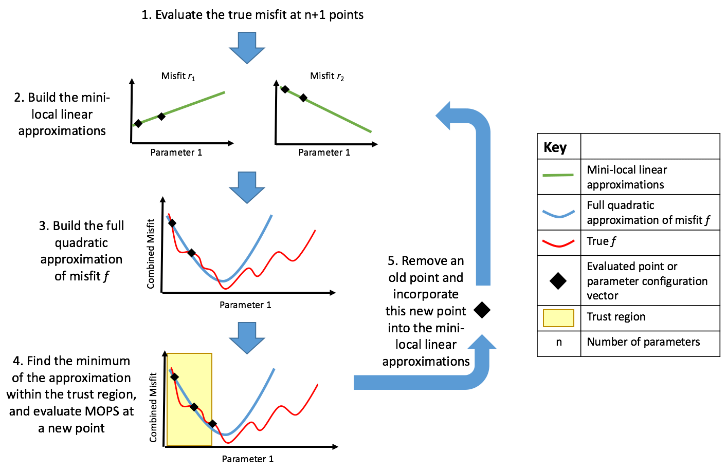
Figure 1 Schematic of DFO-LS optimising one parameter. (1) Two individual misfits r_i are evaluated at two locations in parameter space. (2) Two mini-local regressions are built (green lines) using these two r_i points (black diamonds). (3) These linearised misfits are then squared and summed over to give a quadratic approximation (blue line) to the true misfit function. (4) Within the trust region (shaded in yellow) the minimum of the approximation is found, at which the true misfit function is evaluated. (5) If the new point is accepted, this new information is used to update the mini-local regressions, otherwise it is rejected and the trust region is shrunk. Steps 2–5 are then repeated until the specified termination criterion or maximum evaluations is reached.

2.4.2 DFO-LS

Derivative-free optimisation using least squares (DFO-LS) is an iterative algorithm for minimising a function f(x) (Cartis et al., 2019), where x is the n-dimensional vector of parameters, each of which is constrained within specified bounds. DFO-LS can take into account individual terms of the misfit function and use their structure to improve convergence. Mathematically, DFO-LS solves the nonlinear least-squares problem:

$$\begin{array}{}\text{(1)}& \underset{\mathit{x}\in D}{\text{min}}f\left(\mathit{x}\right)=\sum _{i=\mathrm{1}}^d{r}_{\mathrm{i}}(\mathit{x}{)}^{\mathrm{2}},\end{array}$$

where D is a bounded domain of ℝⁿ, and r_i(x) denotes individual terms in the misfit function. DFO-LS starts at an initial location within the parameter space and then moves through the space to provably find a local minimum (see Appendix A.2 in Cartis et al., 2019, for convergence and complexity rates). The algorithm is illustrated in Fig. 1 and summarised in Appendix B.

DFO-LS must be given a starting location within the parameter space from which to initialise. In the initial iteration of DFO-LS, the misfit function is evaluated at the starting location and at n additional locations nearby (where n is the number of parameters to be optimised), with their proximity determined by DFO-LS settings (see Table B1). In subsequent iterations, typically only one function evaluation is needed, and often only a handful are needed to achieve significant misfit reduction.

Using this set of evaluated points, DFO-LS creates a quadratic approximation to the underlying true (unknown) misfit function (Cartis et al., 2019) and calculates the minimum of this function within a “trust region” centred around the starting point. The true misfit function is then evaluated at this location. If it is found to be worse than the misfit at the existing n+1 points, it is rejected. The trust region is shrunk and the procedure is repeated. On the other hand, if it is found to be lower than the best of the n+1 points then it is accepted, and the point corresponding to the highest misfit amongst the previous n+1 points is discarded. A new quadratic approximation is calculated for this n+1 set of points, and the procedure is repeated. Thus, at any iteration DFO-LS keeps track of n+1 points in parameter space and the point with the lowest misfit is considered as that iteration's best set of parameters. The algorithm is terminated based on three specified criteria: (1) the maximum allowed number of function evaluations is exceeded, (2) the trust region radius is shrunk below a specified size, and (3) misfit reduction progress is identified as being too slow.

Unlike CMA-ES, DFO-LS is more of a “local” optimisation method. However, there is strong numerical evidence from the derivative-free optimiser Py-BOBYQA, upon which DFO-LS is based (Cartis et al., 2021), that it is able to find global minima. To increase the likelihood of finding the global minimum, DFO-LS can either be manually re-initiated from different starting locations in the parameter space, or automatically “restarted” once it determines that the reduction in the misfit is progressing too slowly. During a restart the trust region expands, allowing DFO-LS to search for points potentially outside the local minimum it may be trapped in, and move towards a lower minimum elsewhere. This can be done by either a “hard” restart, whereby the (expensive) misfit function is re-evaluated at n+1 new locations within the expanded trust region, or by a “soft” restart, whereby DFO-LS only “shifts” some of the current n+1 points in parameter space to geometry-improving points (Cartis et al., 2019). The former is more computationally expensive; therefore we do not use it here, although soft restarts are allowed. To increase confidence that DFO-LS has found the global minimum, we also initiate from multiple starting points.

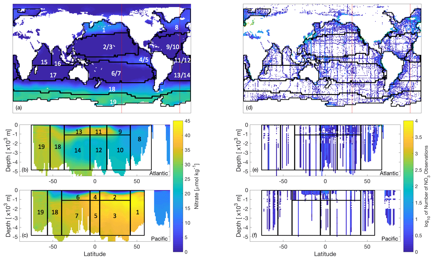
Figure 2 World Ocean Atlas nitrate data (Garcia et al., 2018a, b) of (a–c) interpolated objectively analysed mean concentration of nitrate in sea water [µmol kg⁻¹], and (d–f) number of true observations plotted on a log₁₀ colour scale (white oceanic areas show areas of no nitrate observations). These have been plotted for the (a, d) global surface at 0 m, which also show the locations of the longitudinal transects (red lines) for the nitrate data plotted at (b, e) 23^∘ W and (c, f) 140^∘ W. Overlain are the boundaries of 13 biomes of similar biogeochemistry, the majority of which were determined as in Henson et al. (2010), while those in the Southern Ocean as in Weber et al. (2016). Six regions have been further split by depth, leading to a total of 19 regions.

2.5 Misfit functions

Every evaluation of our misfit requires running the biogeochemical model for 3000 years before calculating the misfit between the model outputs and synthetic observations. While both CMA-ES and DFO-LS minimise a single misfit function, DFO-LS can exploit the structure of the misfit function. Thus, if the misfit is defined as per Eq. (1), we only provide CMA-ES with f(x) whereas the individual r_i(x) are supplied to DFO-LS. There is no maximum suggested value for d, the number of r_i terms; therefore the misfit at every grid point within the model domain could be provided to DFO-LS. However, many of the individual r_i misfits would be physically close to each other in the model and therefore will respond similarly to perturbations in the biogeochemical parameters being optimised, which will result in a heavier weighting to this location of the ocean model. To avoid this, we define r_i to take into account the spatial structure of the misfit by partitioning the ocean into previously established biome regions of similar ocean biogeochemical properties (Henson et al., 2010; Weber et al., 2016, provided by Raffaele Bernardello, Barcelona Supercomputing Centre, personal communication, 2018), several of which were further split by depth at 1000 m (see Fig. 2) for a total of 19 regions. For every region j, we further calculate a misfit for each of the three tracers q (phosphate, nitrate, oxygen) used in the optimisation. The objective f(x) is thus composed of $\mathrm{19}\times \mathrm{3}=\mathrm{57}$ terms of the following form:

$$\begin{array}{}\text{(2)}& r_{qj}^{\mathit{ϵ}}\left(\mathit{x}\right)=\sqrt{{\displaystyle \frac{V_j}{V_{\mathrm{global}}}}}{\displaystyle \frac{\sqrt{{\sum }_{i\in j}\left(m_{qi}\right(\mathit{x})-(o_{qi}+{\mathit{ϵ}}_{qi}){)}^{\mathrm{2}}\frac{V_{\mathrm{i}}}{V_j}}}{{\sum }_{i\in j}{o}_{qi}\frac{V_{\mathrm{i}}}{V_j}}},\end{array}$$

where m_qi(x) is the model solution with parameters x at grid point i for tracer q and o_qi the corresponding observation (the synthetic observations provided by a reference run of MOPS). The misfit is normalised by the volume-weighted mean tracer concentration for that region and weighted, first, by individual grid point volumes V_i relative to the volume V_j of region j and, second, by the region's total volume relative to the global ocean volume V_global. Real oceanic observations have a degree of uncertainty associated with them due to spatio-temporal oceanic processes, e.g. from small-scale processes such as unresolved eddies. To account for this we add a noise term ϵ_iq, which is the added noise due to uncertainty associated with tracer q for every grid box i in the model. The total global misfit $f_{\mathrm{T}}^{\mathit{ϵ}}\left(\mathit{x}\right)$ is then defined as

$$\begin{array}{}\text{(3)}& f_{\mathrm{T}}^{\mathit{ϵ}}\left(\mathit{x}\right)=\sum _{q=\mathrm{1}}^{\mathrm{3}}\sum _{j=\mathrm{1}}^{\mathrm{19}}{r}_{qj}^{\mathit{ϵ}}(\mathit{x}{)}^{\mathrm{2}}.\end{array}$$

The total misfit function is broadly similar to Kriest et al. (2017), with the main difference being the incorporation of the 19 biome regions.

The non-noisy equivalent of these misfit terms are r_qj and f_T as in Eqs. (2) and (3) with ϵ=0. We also define “baseline” misfits $r_{qj}^{\mathrm{base}}$ and $f_{\mathrm{T}}^{\mathrm{base}}$, which are the misfits due to the noise alone in the special case where the model outputs equal the observations (in Eq. 2: m_qi=o_qi). $f_{\mathrm{T}}^{\mathrm{base}}$ give an indication of the termination criteria when optimising the model to real noisy oceanic observations, as optimising below this threshold would serve no useful purpose.

To specify a realistic noise field we take the standard deviation variable provided in the World Ocean Atlas database (WOA18 Garcia et al., 2018a, b). Since our misfit is defined with respect to annual mean data we require an annual mean standard deviation without the variability of the seasonal cycle. To do so we take the numerical mean (weighted by number of observations) of the monthly standard deviations reported in the WOA18 dataset for the upper 800 m (phosphate and nitrate) or 1500 m (oxygen), and the annual standard deviation below those depths. These standard deviations fields were linearly interpolated onto the model grid and then multiplied by three different Gaussian noise fields to create three separate noise (ϵ) realisations. The baseline misfit terms $r_{qj}^{\mathrm{base}}$ and $f_{\mathrm{T}}^{\mathrm{base}}$ were calculated as an average over these realisations.

As mentioned above, the “observations” in this study are from a reference simulation of MOPS, hereafter referred to as MOPS-ref, run with the following parameter values: $R_{{\mathrm{O}}_{\mathrm{2}}:\mathrm{P}}=\mathrm{170}$ mmol O₂: mmol P, I_C=24 W m⁻², K_PHY=0.03125 mmol P m⁻³, μ_ZOO=2 d⁻¹, k_ZOO=3.2 (mmol P m⁻³)⁻¹ d⁻¹ and $b^{\ast }=\mathrm{0.858}$ (see Table C1).

2.6 Optimisation experimental design and solver settings

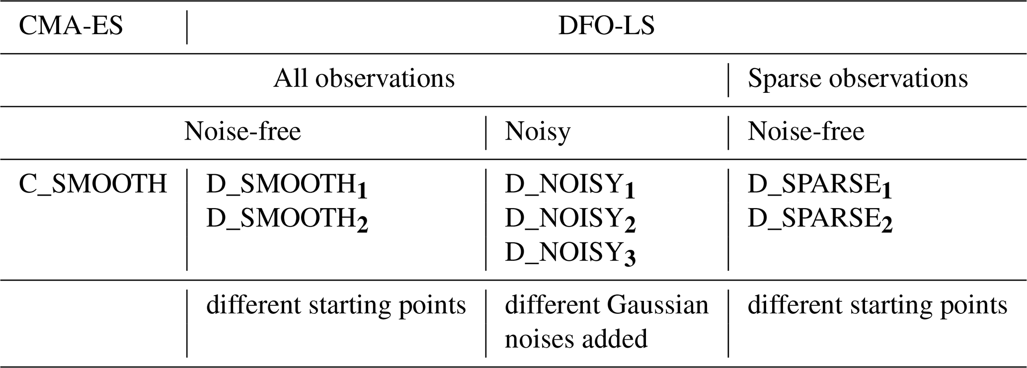
In this study we seek to (1) compare the performance of CMA-ES and DFO-LS on noise-free observations, (2) investigate DFO-LS's performance on noisy observations, and (3) investigate the impact of sparse observations on the ability of DFO-LS to recover the true parameters. In order to do so we carried out the following series of experiments (see Table 1 for the corresponding experiment labels):

Noise-free experiments. In the noise-free experiments we attempted to recover all six parameters. For this a single run of CMA-ES was performed (labelled C_SMOOTH). For DFO-LS two experiments were carried out (D_SMOOTH₁ and D_SMOOTH₂), starting from two different locations in parameter space that were chosen to be relatively far from the target parameters. The parameter values for these and all other experiments are listed in Table C1.

Both CMA-ES and DFO-LS are controlled by various solver settings. For CMA-ES the main ones are the number of sequential generations and the population size. As per Kriest et al. (2017) we set these to 200 and 10, respectively. The solver settings used by DFO-LS are summarised in Table B1. Of the noise-free experiments D_SMOOTH₁ and D_SMOOTH₂, the former had DFO-LS settings regarding trust region management (tr_radius) which are more suitable for a noisy misfit function, while the latter is more suitable for a smooth misfit function. Therefore, D_SMOOTH₁ and D_SMOOTH₂ vary both in starting values and trust region management. As D_SMOOTH₁ was slightly more successful, the trust region management settings were set to be more suitable for a noisy misfit function in all subsequent experiments.

DFO-LS experiments with observational uncertainty. To understand optimisation performance in the presence of observational uncertainty, noise was added to the reference observations (see Sect. 2.5). Three such optimisation runs, each with a different noise realisation, were carried out with DFO-LS (D_NOISY₁, D_NOISY₂, D_NOISY₃) starting from the same location in parameter space, to minimise the noisy misfit function $f_{\mathrm{T}}^{\mathit{ϵ}}$. The goal was to see if DFO-LS could recover all six of the MOPS-ref target parameter values.

DFO-LS experiments with sparse observations. There are large areas of the ocean which have not been sampled adequately or at all (e.g. Fig. 2). While it is possible to fill in the gaps in the data using objective interpolation methods, this might not always work well in the presence of large gradients. In a last set of experiments we therefore compared how DFO-LS performs in the presence of data sparsity (D_SPARSE₁ and D_SPARSE₂), by only using observations at model grid points for which the corresponding locations in WOA18 contain data, with its corresponding performance in the absence of data sparsity (D_SMOOTH₁ and D_SMOOTH₂).

Table 1 Names of each experiment tuning to noise-free, noisy and sparse twin observations. C_SMOOTH is the non-noisy CMA-ES experiment. D_SMOOTH₁ and D_SMOOTH₂ are the non-noisy DFO-LS experiments starting from two different locations in parameter space, run specifically to be compared to C_SMOOTH. D_noise_randi are the noisy DFO-LS experiments, with three different noise realisations, run specifically to be compared to the non-noisy equivalent experiment D_SMOOTH₁. D_SPARSE₁ and D_SPARSE₂ are the non-noisy DFO-LS experiments calibrating to sparse observations, starting from two different locations in parameter space, run specifically to be compared to the non-sparse equivalent experiments D_SMOOTH₁ and D_SMOOTH₂, respectively.

3 Results

3.1 Parameter sensitivities

To provide insight into why some parameters were tuned better or worse in the following optimisation experiments, the sensitivity of the misfit function to an individual perturbation in each parameter has been calculated and shown in Fig. 3. The greatest change in the misfit was caused by perturbing b^∗ by 10 % of its range, followed by I_C. The parameter with the lowest influence on the misfit at this local point in parameter space was K_PHY, in which a 10 % perturbation caused a misfit change of only $\mathrm{4.1}\times {\mathrm{10}}^{-\mathrm{6}}$.

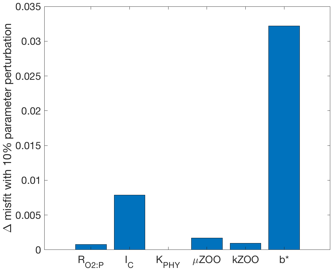
Figure 3 Bar graph of the misfit change due to individual parameter perturbations from their target value to +10 % of their range.

3.2 Noise-free experiments

The results for all twin optimisation experiments are summarised in Figs. 4 and 5, and in Appendix C (Tables C1 and C2), which show the starting and optimised parameter values, and parameter recovery information. In the subsequent sections we then plot both the global misfit and parameter values for every function evaluation throughout each individual optimisation experiment (Figs. 6–13). During one CMA-ES iteration we evaluate the misfit function 10 times (the population size). Therefore for CMA-ES we plot the minimum (best) and maximum misfits, and we plot the parameter values corresponding to the best misfit, and the minimum and maximum parameter values of each population.

To both reiterate how DFO-LS works and fully explain the DFO-LS figures, we briefly describe the optimisation process in terms of expected misfit reduction and parameter trajectories. First, DFO-LS evaluates the misfit function n+1 times near to the chosen starting point; therefore in the first seven evaluations we do not expect a misfit reduction. After these initial evaluations, DFO-LS attempts to minimise the misfit function and there will be both successful evaluations (the resulting misfit is lower than previously found in the optimisation) and unsuccessful ones (the misfit is not lower). There may also be restarts, directly after which unsuccessful evaluations are common as DFO-LS perturbs the parameter values to get out of a possible local minimum. Therefore on every DFO-LS figure we have plotted the misfit or parameter values for every evaluation (both successful and unsuccessful) as scattered points, and successful ones in a solid line.

On every figure of total global misfits the expected baseline misfit ($f_{\mathrm{T}}^{\mathrm{base}}$; see Sect. 2.5) is also plotted, below which any misfit reduction is within observational noise levels. On every parameter trajectory plot the “recovery zone” is also shown. This indicates the range of parameter values within ±5 % of the target value, normalised by the total range (upper bound minus lower bound) for that parameter. We consider a parameter to have been “recovered” by a certain number of evaluations, when all subsequent parameter values corresponding to successful evaluations remain within this recovery zone.

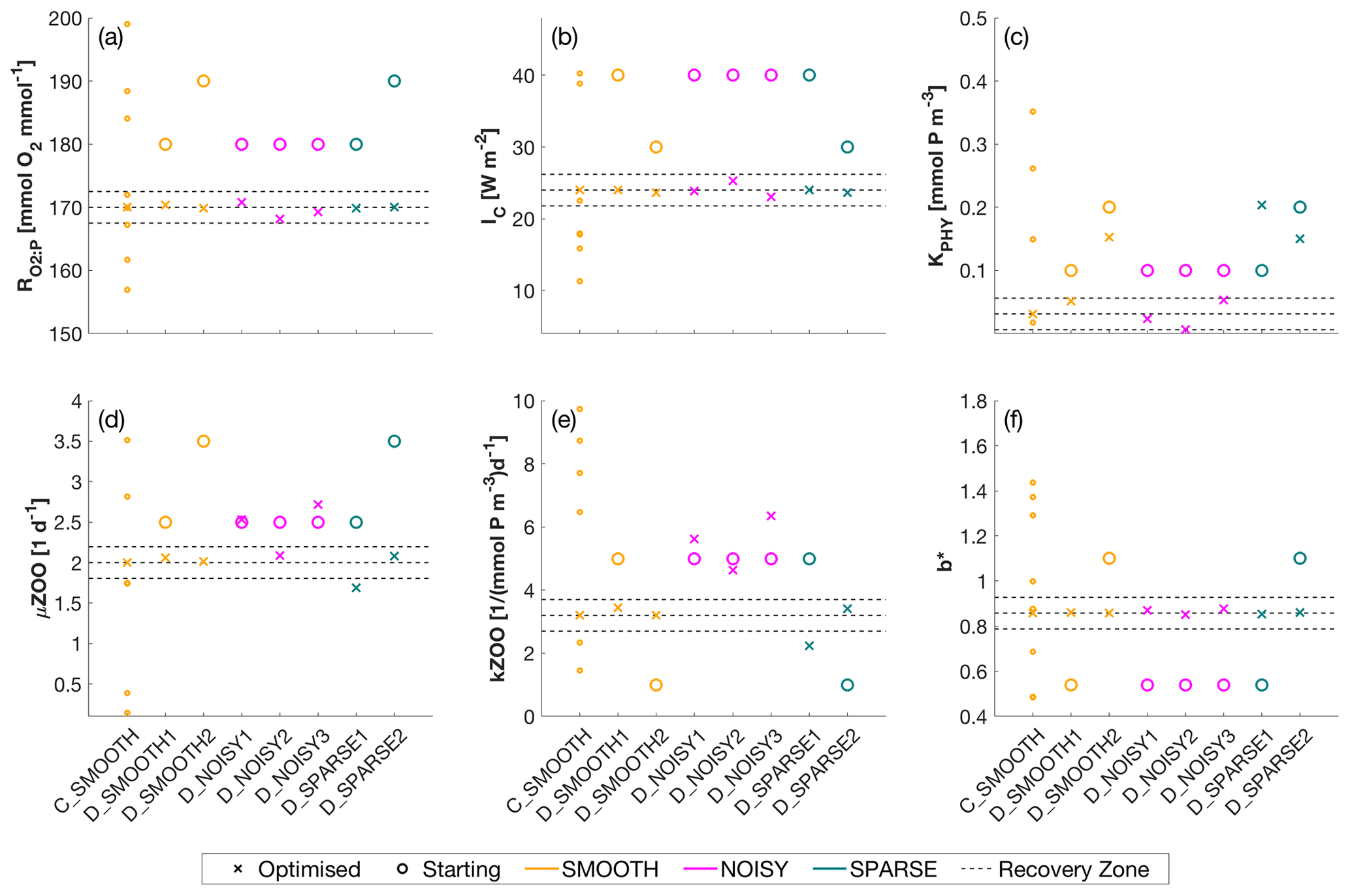
Figure 4 Optimised (cross markers) and starting (circle markers) parameters for all SMOOTH (orange), NOISY (magenta) and SPARSE (green) twin experiments, shown for parameter (a) $R_{{\mathrm{O}}_{\mathrm{2}}:\mathrm{P}}$ [mmol O₂ : mmol P], (b) I_C [W m⁻²], (c) K_PHY [mmol P m⁻³], (d) μ_ZOO [d⁻¹], (e) k_ZOO [(mmol P m⁻³)⁻¹ d⁻¹] and (f) b^∗. For C_SMOOTH multiple starting locations (small orange markers) are shown, as unlike DFO-LS, CMAES selects 10 unconstrained randomised starting points. As CMA-ES is unconstrained, not all starting locations plot within the parameter bounds, to which the y-axis limits are fixed. Also plotted are the MOPS-ref target parameter values and ±5 % recovery zone (horizontal black dashed lines). For further information see Table C1.

Figure 5 Number of evaluations required by the SMOOTH (orange), NOISY (magenta) and SPARSE (green) twin experiments to (a) reduce the global misfit to below noise levels (baseline misfit) and (b–g) successfully recover each parameter. The red dashed line shows the maximum number of evaluations allowed for DFO-LS experiments. Black arrows indicate (a) the baseline misfit was not reached, or (b–g) the parameter was not recovered in that optimisation experiment. Note that the number of evaluations required by CMA-ES in experiment C_SMOOTH always plotted above the break in the y axis. For further information see Table C2.

CMA-ES experiment. Figure 6 shows that during the optimisation C_SMOOTH by CMA-ES the global misfit decreases significantly from 10⁻¹ to $\approx {\mathrm{10}}^{-\mathrm{4}}$ within the first 500 function evaluations. Subsequently progress slows down as the misfit is reduced by only 1 more order of magnitude over the next 1000 evaluations. Progress then significantly improves, with the misfit decreasing from $\approx {\mathrm{10}}^{-\mathrm{5}}$ to 10⁻⁹ within the final 500 evaluations. Note that the spikes in the maximum global misfit near the 1650th evaluation was due to the added penalty factor when one of the parameter values in this population had a value just outside of its allowed range. While this experiment did not include noise, we note that CMA-ES required 309 evaluations to reach the baseline misfit, beyond which any misfit reduction would have been within observational noise levels.

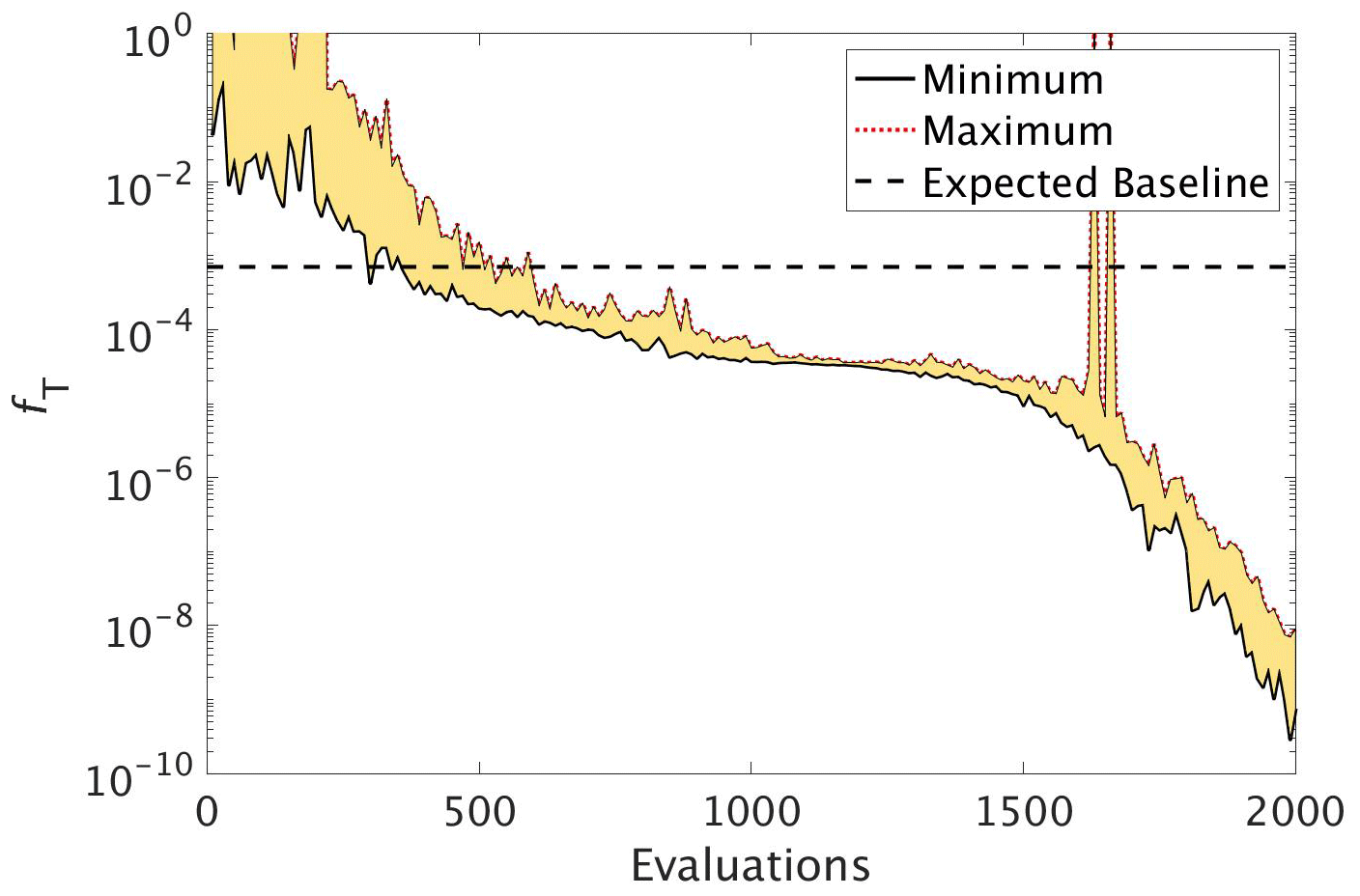
Figure 6 The reduction in global misfit of MOPS to the twin MOPS-ref observations by CMA-ES for the experiment C_SMOOTH. There were 10 MOPS evaluations within each CMA-ES iteration (population λ=10), ran in parallel. Plotted is the baseline (horizontal black dashed line), minimum (black solid line) and maximum (red dotted line) misfit of each population, with the area between shaded yellow.

Figure 7 shows how the six parameters were optimised towards the MOPS-ref target parameter values by CMA-ES. The targets were found relatively quickly within the initial 500 evaluations for the parameters $R_{{\mathrm{O}}_{\mathrm{2}}:\mathrm{P}}$, I_C and b^∗, corresponding to the initial fast misfit reduction previously shown in Fig. 6. The μ_ZOO and k_ZOO targets were found next after approximately 1000 evaluations, after which the optimiser began tuning K_PHY towards its target until it located after 1700 evaluations. If C_SMOOTH had been terminated once the observational noise level was reached after 309 evaluations, $R_{{\mathrm{O}}_{\mathrm{2}}:\mathrm{P}}$, I_C and b^∗ would have been optimised to their MOPS-ref values relatively well, while K_PHY, μ_ZOO and k_ZOO would still be far from their target values.

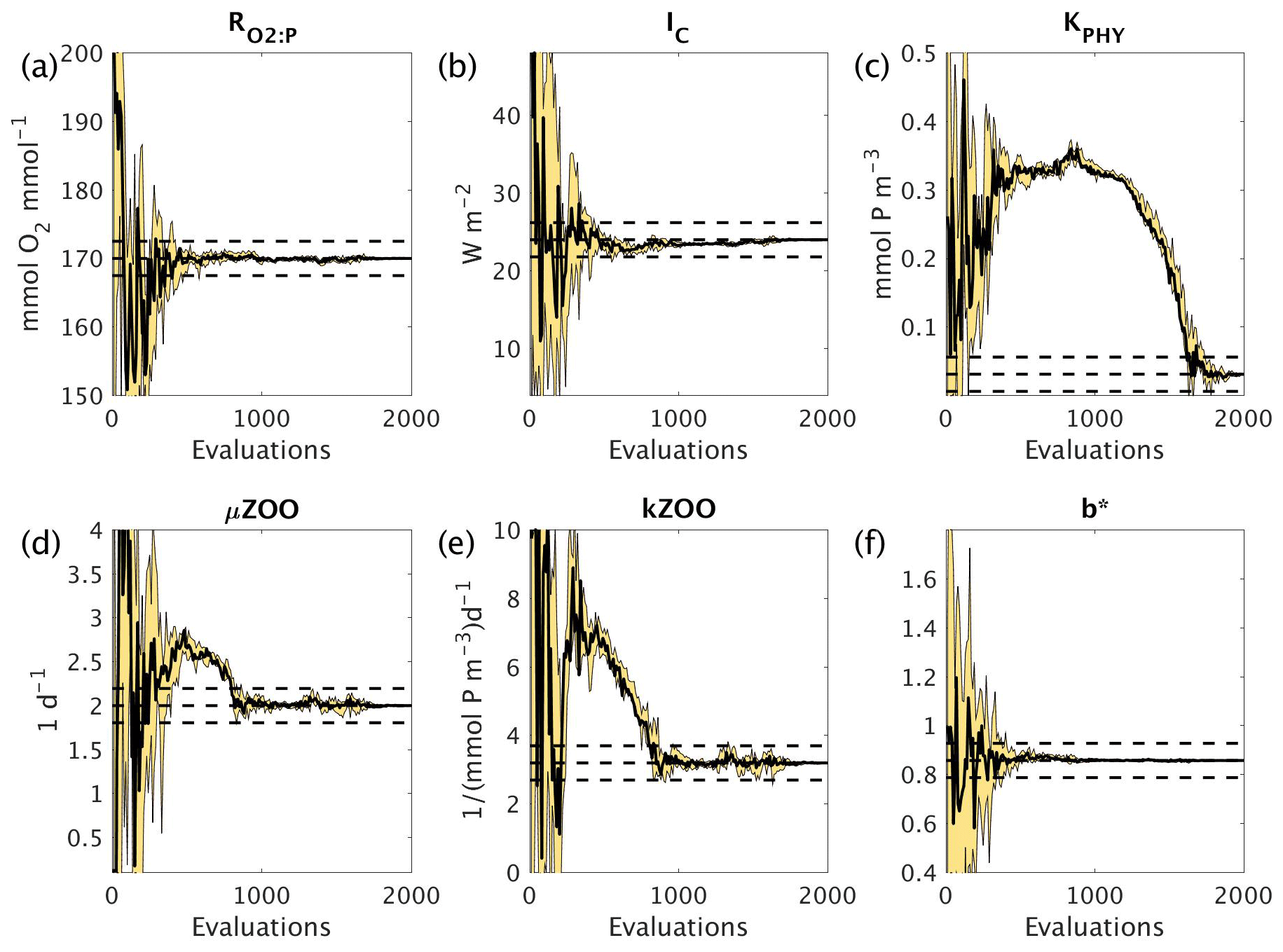
Figure 7 Parameter tuning by CMA-ES for the experiments C_SMOOTH for the parameters (a) $R_{{\mathrm{O}}_{\mathrm{2}}:\mathrm{P}}$, (b) I_C, (c) K_PHY, (d) μ_ZOO, (e) k_ZOO and (f) b^∗. There were 10 MOPS evaluations within each CMA-ES iteration (population λ=10), run in parallel. Plotted are the parameter values associated with the minimum misfit of that population (thick black solid line), and the maximum and minimum of all parameter values within that population (thin black solid lines), with the area between shaded yellow. Also plotted are the MOPS-ref target parameter values and ±5% recovery zone (horizontal black dashed lines).

DFO-LS experiments. To compare the performance of DFO-LS with CMA-ES we carried out two optimisation experiments with DFO-LS (D_SMOOTH₁ and D_SMOOTH₂) starting from two different locations in parameter space, with differing parameters controlling the DFO-LS trust region shrinking speed. Optimisation D_SMOOTH₁ had slower trust region shrinking settings to allow it to better handle an irregular misfit function. Figure 8 shows the comparison between both experiments' reduction of the global misfit. In both cases there was rapid initial misfit decrease from near 10⁻¹ to 10⁻³ within 30 model evaluations. Optimisation D_SMOOTH₂ showed slightly slower misfit reduction, needing 35 evaluations to reach the baseline misfit, while D_SMOOTH₁ only required 20 to reach the baseline, beyond which any misfit reduction is within observational noise levels. In both D_SMOOTH₁ and D_SMOOTH₂ DFO-LS managed to reduce the misfit to below 10⁻⁵ within 45–49 evaluations and then initiated restarts to reduce it further. As D_SMOOTH₁ performed slightly better than D_SMOOTH₂, especially between evaluations 15–45, D_SMOOTH₁ trust region shrinking settings were used as defaults for all subsequent experiments.

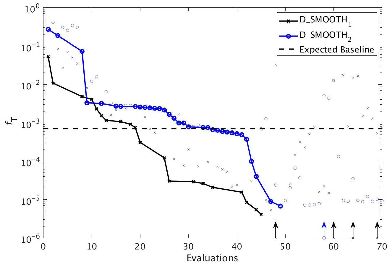
Figure 8 The reduction in global misfit of MOPS to the twin MOPS-ref observations by DFO-LS for the experiments D_SMOOTH₁ (black line with crosses) and D_SMOOTH₂ (blue line with circles). Also plotted is the baseline misfit (horizontal black dashed line). Vertical arrows indicate a soft restart, coloured and marked according to each experiment. Note that every MOPS evaluation has been plotted with a small marker; however, only MOPS evaluations which resulted in a lower misfit than previously seen in each optimisation experiment have been plotted with a solid line.

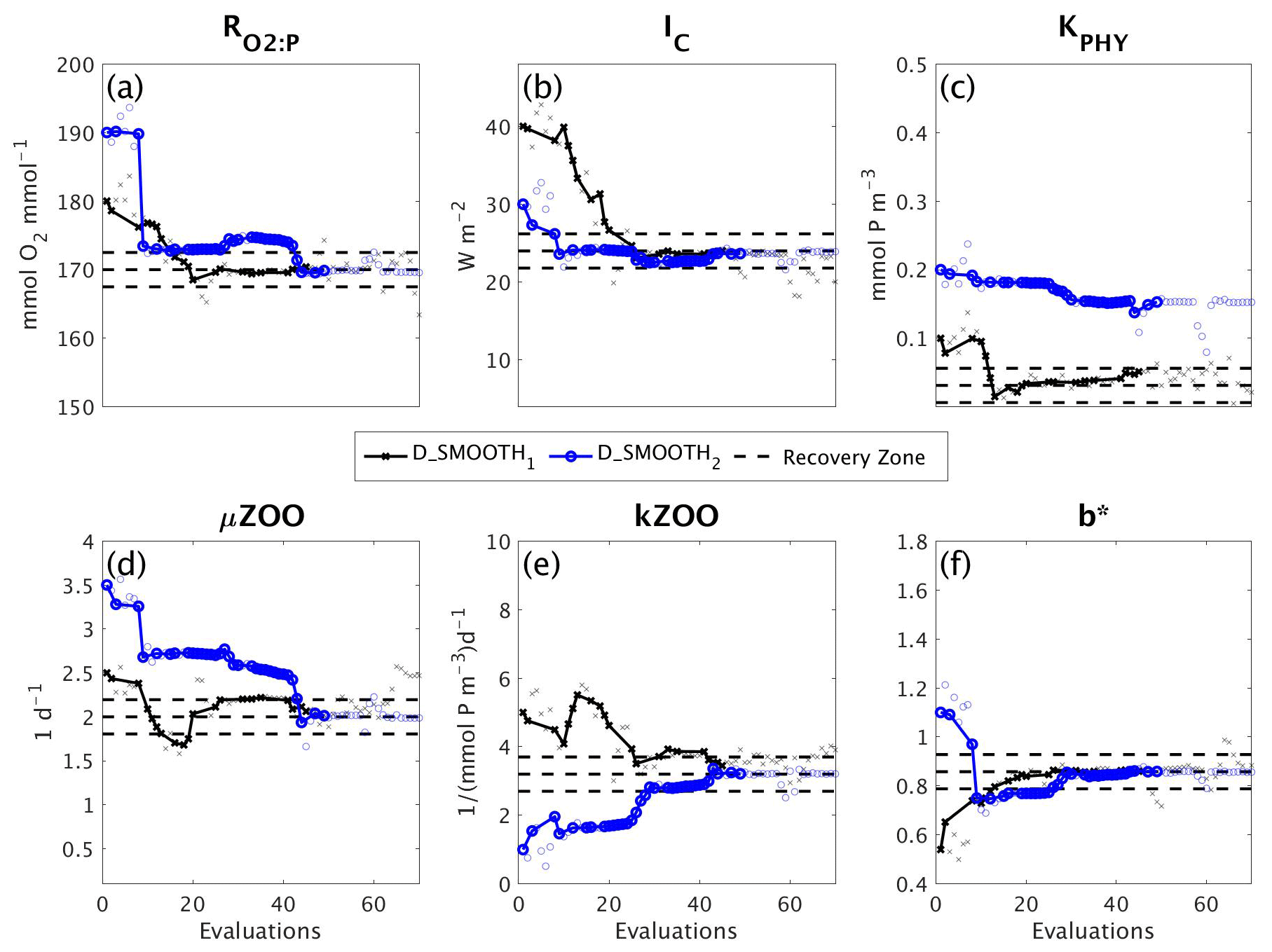
Figure 9 Parameter tuning by DFO-LS for the experiments D_SMOOTH₁ (black line with crosses) and D_SMOOTH₂ (blue line with circles) for the parameters (a) $R_{{\mathrm{O}}_{\mathrm{2}}:\mathrm{P}}$, (b) I_C, (c) K_PHY, (d) μ_ZOO, (e) k_ZOO and (f) b^∗. Also plotted are the MOPS-ref target parameter values and ±5% recovery zone (horizontal black dashed lines). Note that every MOPS evaluation has been plotted with a small marker; however, only MOPS evaluations which resulted in a lower misfit than previously seen in each optimisation experiment have been plotted with a solid line.

Figure 9 shows how the six parameters were optimised towards the MOPS-ref target parameter values by D_SMOOTH₁ and D_SMOOTH₂. In both experiments within the first 30 evaluations $R_{{\mathrm{O}}_{\mathrm{2}}:\mathrm{P}}$, I_C, k_ZOO and b^∗ were optimised to relatively close to their targets, and μ_ZOO within the first 45 evaluations. The parameter the misfit function was least sensitive to, K_PHY, was successfully optimised by D_SMOOTH₁; however, was not successfully optimised at all by D_SMOOTH₂. If D_SMOOTH₁ and D_SMOOTH₂ had been terminated once reaching the noise baseline, after 20 and 35 evaluations respectively, $R_{{\mathrm{O}}_{\mathrm{2}}:\mathrm{P}}$, I_C, b^∗ and k_ZOO would have been optimised to their MOPS-ref values relatively well.

3.3 DFO-LS experiments with observational uncertainty

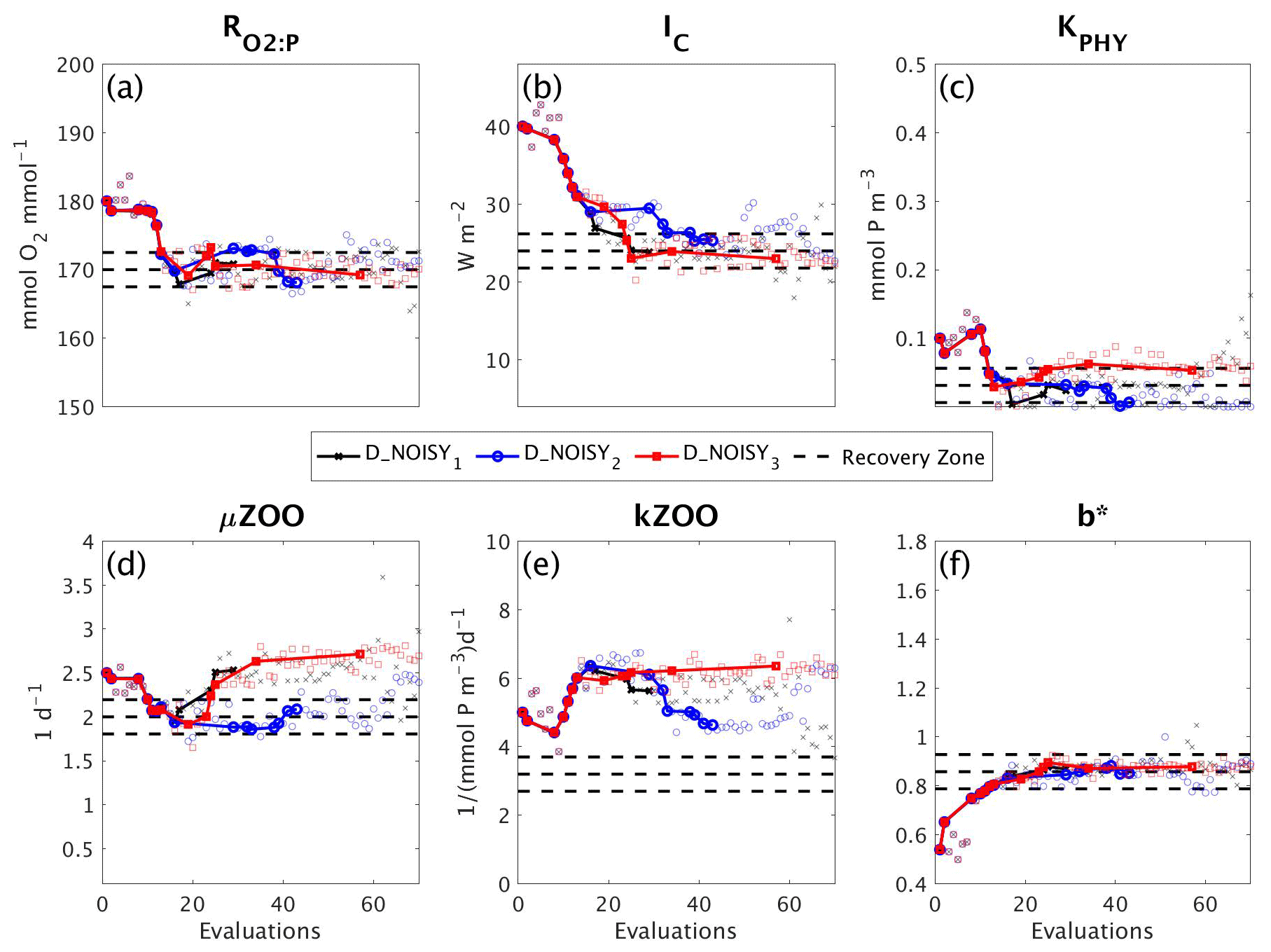
To assess the impact of observational uncertainty we carried out three experiments in which DFO-LS was initialised from the same starting location in parameter space, but with three different realisations of random noise added to the observations (see Sect. 2.6). As seen in Fig. 10 DFO-LS managed to reduce the misfit to very close to the average baseline misfit within 30 evaluations with a reduction in misfit from $\sim {\mathrm{10}}^{-\mathrm{1}}$ to $\sim {\mathrm{10}}^{-\mathrm{3}}$. Closer to the end of the optimisation runs, restarts were initiated to encourage further misfit reduction, hence the large variations in misfit. Figure 11 shows that the initial misfit reduction corresponds to improved values for the parameters $R_{{\mathrm{O}}_{\mathrm{2}}:\mathrm{P}}$, I_C, K_PHY and b^∗. DFO-LS seems to compensate for the noise by increasing the values for the parameters μ_ZOO and k_ZOO.

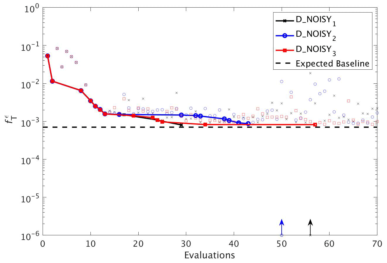
Figure 10 As in Fig. 8, but for experiments D_NOISY₁ (black line with crosses), D_NOISY₂ (blue line with circles) and D_NOISY₃ (red line with squares). Vertical arrows indicate a soft restart, coloured and marked according to each experiment.

Figure 11 As in Fig. 9, but for the experiments D_NOISY₁ (black line with crosses), D_NOISY₂ (blue line with circles) and D_NOISY₃ (red line with squares).

3.4 DFO-LS experiments with sparse observations

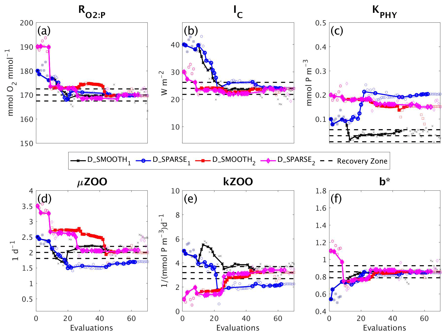
In a final set of experiments we examine whether DFO-LS is able to successfully optimise MOPS given a sparse set of observations (see Sect. 2.6). The experiments D_SPARSE₁ and D_SPARSE₂ were initialised from the same location in parameter space as D_SMOOTH₁ and D_SMOOTH₂, respectively, but the former were optimised using observations sub-sampled at grid points corresponding to locations in the un-interpolated WOA18 database. In these experiments no noise was added to the observations. Figure 12 shows that the two optimisations using full observations (D_SMOOTH₁ and D_SMOOTH₂) converged to slightly lower misfits than when using sparse observations. Figure 13 shows that D_SMOOTH₁ successfully recovered all six parameters within 42 evaluations, while D_SPARSE₁ only successfully recovered $R_{{\mathrm{O}}_{\mathrm{2}}:\mathrm{P}}$, I_C and b^∗ throughout the optimisation. The above results would indicate a poorer optimisation when using sparse observations; however, when starting from a different location in parameter space, D_SMOOTH₂ successfully recovered five parameters within 44 evaluations, while D_SPARSE₂ recovered the same five after only 26 evaluations. This suggests that even with sparse observations it is possible to successfully optimise a global ocean biogeochemical model such as MOPS.

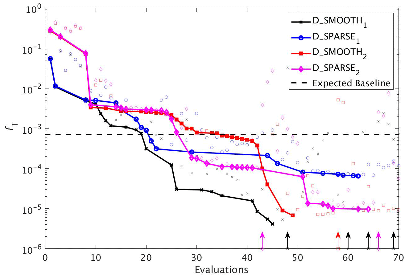
Figure 12 As in Fig. 8, but for experiments D_SMOOTH₁ (black line with crosses), D_SPARSE₁ (blue line with circles), D_SMOOTH₂ (red line with squares) and D_SPARSE₂ (magenta line with diamonds). Vertical arrows indicate a soft restart, coloured and marked according to each experiment. Note that the baseline misfit (horizontal black dashed line) was calculated using the full grid noisy observations.

Figure 13 As in Fig. 9, but for the experiments D_SMOOTH₁ (black line with crosses), D_SPARSE₁ (blue line with circles), D_SMOOTH₂ (red line with squares) and D_SPARSE₂ (magenta line with diamonds).

4 Discussion

4.1 CMA-ES vs. DFO-LS optimisation performance

Our comparison of the two optimisation algorithms shows that DFO-LS could recover all six target parameter values within ∼40 evaluations of MOPS, while CMA-ES achieved the same goal within ∼1700 evaluations. By “recover” we mean optimised to within ±5 % (normalised by the parameter range) of the target value. DFO-LS reduced the misfit to below the observational uncertainty threshold within 20–35 evaluations, while CMA-ES required 309 evaluations. DFO-LS is thus significantly more efficient for this particular problem and may, in general, be more practical for optimising more than a small handful of parameters. However, we note that the multiple evaluations CMA-ES requires can be run in parallel. In contrast, DFO-LS, except for the initial n+1 evaluations, runs sequentially.

CMA-ES is a single-objective optimiser, while DFO-LS can use information from multiple misfit values instead of just one. Therefore it can exploit more information to allow for a faster reduction in the misfit. Neither algorithm can completely guarantee a global optimum solution, although CMA-ES carries out a more global search than DFO-LS. There is significant evidence DFO-LS can find the global optimum (Cartis et al., 2021), but to increase confidence in the final solution it can be combined with a globalising method such as starting from different points in parameter space or using the DFO-LS restart functionality.

Both methods struggled with one of the parameters K_PHY, due to the misfit function's low sensitivity to this parameter (as found by perturbing the parameter values in each direction and computing the gradient). DFO-LS had not begun to tune this parameter for one of the experiments (D_SMOOTH₂) before we terminated it at a maximum of 70 evaluations, although it did find K_PHY when initiated from a different starting point (D_SMOOTH₁). CMA-ES also had difficulty in tuning K_PHY and only started optimising this parameter after all the other parameters were recovered at ∼1200 evaluations. The maximum number of DFO-LS evaluations was set to 70 as it is a sequential algorithm; therefore it was impractical to allow too many more evaluations. Had it been allowed to run longer the expectation is it would begin tuning K_PHY once the other five were sufficiently tuned, as was the case with CMA-ES. However, the computational expense of continuing DFO-LS to recover K_PHY was deemed too costly, particularly due to the fact that this parameter has so little influence on the misfit function and therefore did not impact the successful misfit reduction achieved by DFO-LS. This low sensitivity to K_PHY was also seen by Kriest et al. (2017), who determined the surface observations contribute too little to the total misfit, rendering the misfit function insensitive to perturbations in parameters that mainly influence the surface ocean (e.g. K_PHY). To help overcome this in future work, one could put more weighting on surface data when formulating the misfit.

4.2 Calibrating to uncertain observations

Real oceanic observations come with associated uncertainty due to measurement error, temporal variations such as seasonal and diurnal cycles, and meso-scale variability due to factors such as eddies and the movement of fronts. Here we have studied how this uncertainty raises the base of the misfit function, below which any optimisation of the biogeochemical model would be within the uncertainty level. We determined this baseline for the misfit function (or termination threshold) using the standard deviations of the observational data; however, others have defined it as the global optimum of a surrogate formulation of the biogeochemical model (Sauerland et al., 2017). In the present case and with the chosen set of oceanic observations, the model was significantly optimised before reaching levels of observational uncertainty, particularly due to optimisation of the parameters which the model is most sensitive to, as was determined by perturbing each parameter while holding the others fixed and calculating the misfit. In this case it was I_C (the phytoplankton half-saturation for light) and b^∗ (the increase in particle sinking speed with depth). Somewhat surprisingly, a parameter the model is less sensitive to, $R_{{\mathrm{O}}_{\mathrm{2}}:\mathrm{P}}$ (the ratio of oxygen consumption to phosphate release during remineralisation), was also well optimised before reaching the baseline. Despite the low sensitivity, possibly caused by narrow parameter bounds, the high optimisation potential by this parameter may be due to the fact that the misfit function includes both oxygen and phosphate. It could also be due to the fact that this parameter has a non-local effect, as it influences the flux of oxygen and phosphate to the deeper ocean, hence to ocean basins further along the “conveyor belt”. This is also the case for b^∗ (Kwon and Primeau, 2006; Kriest et al., 2012) but even more so as it also influences the vertical flux of all three of the tracers. In order to optimise less sensitive parameters before reaching noise levels one could introduce more metrics into the misfit calculation to help constrain these parameters, for example phytoplankton and zooplankton data, or additional oxygen constraints, such as the location of oxygen minimum zones as done by Niemeyer et al. (2019).

4.3 Calibrating to sparse observations

We also investigated the ability of DFO-LS to optimise MOPS in the presence of sparsity in the observational data. The results shown here suggest that there is no significant difference in the performance of DFO-LS when tuning to data at every grid point versus a subset of grid points, in line with earlier findings by Kriest et al. (2010). Interpolating can introduce large errors, on the order of 20 % (Garcia et al., 2018a, b), particularly in poorly sampled regions such as the Southern Ocean. However, our experiments suggest that it is possible to use un-interpolated observations, but it is important to start the optimiser from multiple locations in parameter space, or to generously allow restarts, in the presence of a complex misfit function with many local minima. These multiple runs clearly can be run in parallel.

5 Summary

This study compared the efficiency and performance of two derivative-free optimisation algorithms, CMA-ES and DFO-LS, applied to MOPS, a global ocean biogeochemical model with seven prognostic tracers. The two methods were used to tune six of the parameters that control the behaviour of MOPS. We found that DFO-LS has a significantly lower computational cost when compared to CMA-ES, between one and two orders of magnitude, which is important considering that global ocean biogeochemical models are computationally expensive, as they must be integrated for several thousand years to reach equilibrium. DFO-LS exploits more information when minimising the misfit function and therefore has more scope for reducing the misfit faster than CMA-ES. However, as DFO-LS is more of a local optimiser than CMA-ES, it should be paired with a globalising method such as starting from different initial points in parameter space, which can easily be run in parallel.

Future work will involve applying DFO-LS to tune the MEDUSA biogeochemical model (Yool et al., 2011, 2013) to real observations. MEDUSA is more typical of the biogeochemical models which are embedded within earth system models (in the case of MEDUSA, UKESM) that are used to project climate change.

Appendix A: CMA-ES algorithm description

Below is a simplified description of the (μ/μ_W,λ)-CMA-ES algorithm (Hansen, 2016).

Algorithm A1 (μ/μ_W,λ)-CMA-ES.

0:

1:

INPUT: Set initial parameters as in Table 1 of Kriest et al. (2017), population size λ=10, $\mathit{\mu }=\mathit{\lambda }/\mathrm{2}$, evolution paths, covariance matrix C=I, distribution mean, step size and maximum generation number.

1:

while maximum generation is not reached and fitness distribution is not flat do

2:

Sample population of new probability distribution

3:

for $k=\mathrm{0},\mathrm{1},\mathrm{2},\mathrm{\dots }\mathit{\lambda }$ do

4:

Sample search point for this k

5:

end for

6:

Update probability distribution

7:

Update the mean of the search distribution according to a weighted average of the best half of the previously sampled population

8:

Update the overall standard deviation (“step size”)

9:

Update evolution paths

10:

Update covariance matrix

11:

end while

Appendix B: DFO-LS algorithm description

Below is a simplified description of the DFO-LS algorithm in the context of how it has been used in this study. Not all technical details are included, such as safeguarding steps to improve the geometry of points and the quality of the model; therefore see the full description in Cartis et al. (2019).

Table B1 DFO-LS parameter settings for each optimisation experiment. All parameter settings are described in full in the DFO-LS user manual, which is available for download alongside the DFO-LS software. * Group A: all experiments excluding D_SMOOTH₂.

Algorithm B1 DFO-LS.

Require:

Number of parameters n, starting point x₀∈ℝⁿ, minimum trust region radius (p_end), if hard or soft restarts are allowed (see Sect. 2.4.2), and maximum number of true misfit function evaluations.

1:

Evaluate the true misfit function at n+1 points within the initial trust region to build the initial interpolation set {Y₀} (this can be done in parallel).

2:

for $k=\mathrm{0},\mathrm{1},\mathrm{2},\mathrm{\dots }$ do

3:

if we have exceeded the maximum number of true misfit function evaluations then

4:

terminate.

5:

end if

6:

Construct a quadratic approximation of the true misfit function.

7:

Approximately solve the trust region subproblem to locate the minimum of the approximation within the trust region and get step s_k to this point.

8:

Evaluate the true misfit function at x_k+s_k.

9:

if the misfit is significantly decreased then

10:

Accept Step:

11:

Set ${\mathit{x}}_{k+\mathrm{1}}={\mathit{x}}_k+{\mathit{s}}_k$.

12:

if misfit decrease is not significant then

13:

call a hard or soft restart if allowed, or terminate.

14:

end if

15:

Form {Y_k+1} by replacing the worst point with the new accepted point to maintain a set of n+1 points.

16:

else

17:

Reject Step:

18:

Set ${\mathit{x}}_{k+\mathrm{1}}={\mathit{x}}_k$ and shrink the trust region.

19:

if the trust region radius is smaller than p_end then

20:

call a hard or soft restart if allowed, or terminate.

21:

end if

22:

Make $\mathit{\left\{}{\mathit{Y}}_{k+\mathrm{1}}\mathit{\right\}}=\mathit{\left\{}{\mathit{Y}}_k\mathit{\right\}}$.

23:

end if

24:

end for

Appendix C: Optimisation results tables

Table C1 Optimised parameters for all twin experiments. Upper section shows parameter bounds and MOPS-ref target parameters to be recovered. Lower section shows each experiment's results. Columns 2–7: (first row) starting parameter values and (second row) optimised parameters for $R_{{\mathrm{O}}_{\mathrm{2}}:\mathrm{P}}$ [mmol O₂ : mmol P], I_C [W m⁻²], K_PHY [mmol P m⁻³], μ_ZOO [d⁻¹], k_ZOO [(mmol P m⁻³)⁻¹ d⁻¹] and b^∗. Column 8: (first row) the starting global misfit and (second row) the lowest global misfit. n/a: not applicable for CMA-ES.

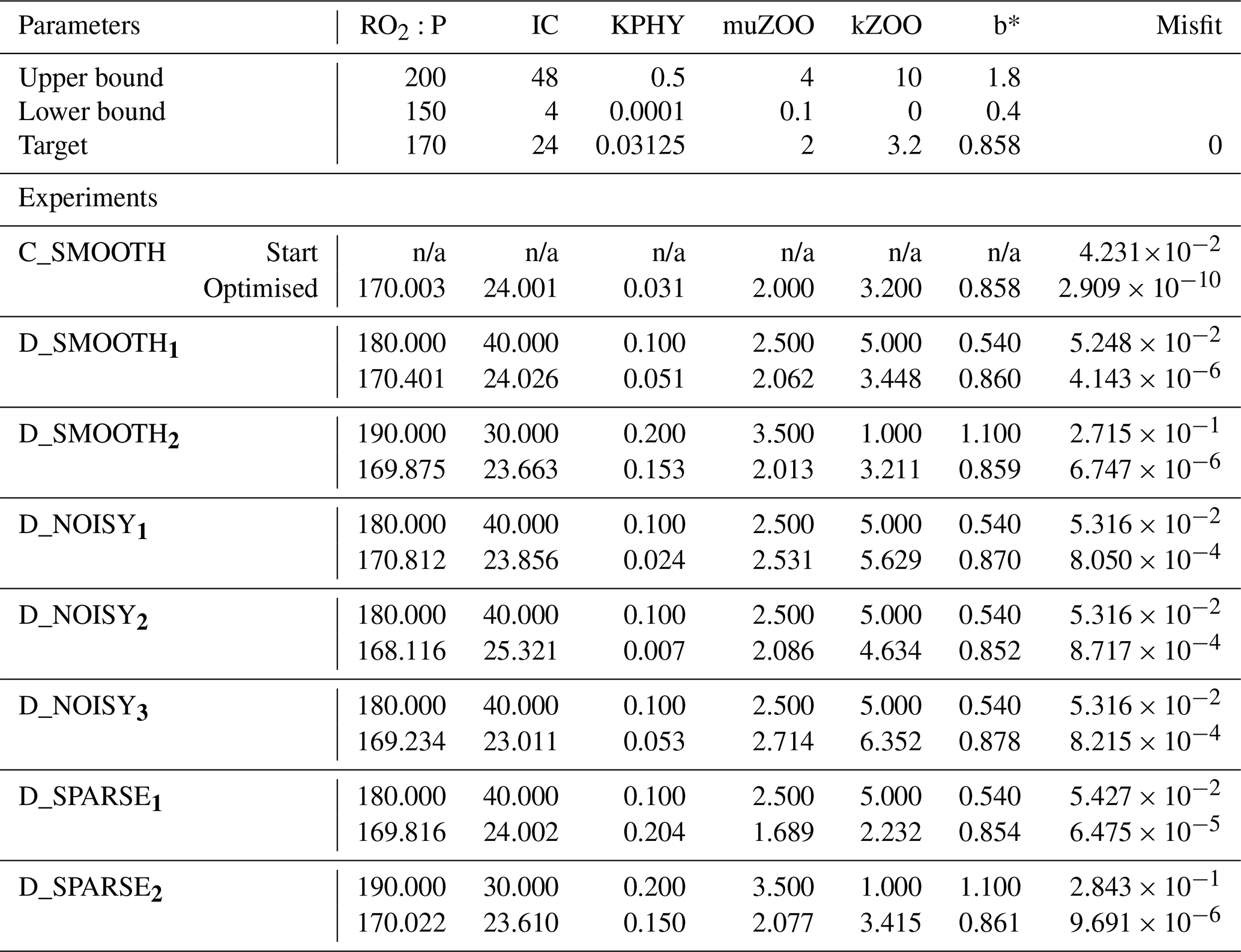
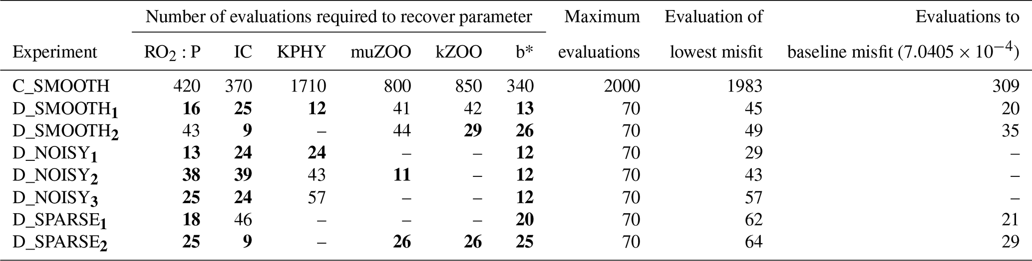
Table C2 Number of evaluations required to recover each parameter for all twin experiments. Columns 2–7: number of misfit function evaluations required to successfully recover that parameter (“–”: never recovered). All evaluations required to recover a parameter which were fewer than 40 are typed in bold font. Column 8: the maximum number of evaluations completed. Column 9: the evaluation which provided the lowest or “best” global misfit. Column 10: the number of evaluations needed for the global misfit to be reduced below noise levels (“–”: never reached the baseline).