KGML-ag: a modeling framework of knowledge-guided machine learning to simulate agroecosystems: a case study of estimating N₂O emission using data from mesocosm experiments

Agricultural nitrous oxide (N₂O) emission accounts for a non-trivial fraction of global greenhouse gas (GHG) budget. To date, estimating N₂O fluxes from cropland remains a challenging task because the related microbial processes (e.g., nitrification and denitrification) are controlled by complex interactions among climate, soil, plant and human activities. Existing approaches such as process-based (PB) models have well-known limitations due to insufficient representations of the processes or uncertainties of model parameters, and due to leverage recent advances in machine learning (ML) a new method is needed to unlock the “black box” to overcome its limitations such as low interpretability, out-of-sample failure and massive data demand. In this study, we developed a first-of-its-kind knowledge-guided machine learning model for agroecosystems (KGML-ag) by incorporating biogeophysical and chemical domain knowledge from an advanced PB model, ecosys, and tested it by comparing simulating daily N₂O fluxes with real observed data from mesocosm experiments. The gated recurrent unit (GRU) was used as the basis to build the model structure. To optimize the model performance, we have investigated a range of ideas, including (1) using initial values of intermediate variables (IMVs) instead of time series as model input to reduce data demand; (2) building hierarchical structures to explicitly estimate IMVs for further N₂O prediction; (3) using multi-task learning to balance the simultaneous training on multiple variables; and (4) pre-training with millions of synthetic data generated from ecosys and fine-tuning with mesocosm observations. Six other pure ML models were developed using the same mesocosm data to serve as the benchmark for the KGML-ag model. Results show that KGML-ag did an excellent job in reproducing the mesocosm N₂O fluxes (overall r²=0.81, and RMSE=3.6 $\mathrm{mg}\mathrm{N}{\mathrm{m}}^{-\mathrm{2}}{\mathrm{d}}^{-\mathrm{1}}$ from cross validation). Importantly, KGML-ag always outperforms the PB model and ML models in predicting N₂O fluxes, especially for complex temporal dynamics and emission peaks. Besides, KGML-ag goes beyond the pure ML models by providing more interpretable predictions as well as pinpointing desired new knowledge and data to further empower the current KGML-ag. We believe the KGML-ag development in this study will stimulate a new body of research on interpretable ML for biogeochemistry and other related geoscience processes.

1 Introduction

Nitrous oxide (N₂O), with its global warming potential 273±118 times greater than that of carbon dioxide (CO₂) for a 100-year time horizon, is one of the major greenhouse gases (IPCC6; Forster et al., 2021). The increasing rate of atmospheric N₂O concentration during the period 2010–2015 is 44 % higher than during 2000–2005, mainly driven by increased anthropogenic sources that have increased total global N₂O emissions to ∼17 Tg N yr⁻¹ (Syakila and Kroeze, 2011; Thompson et al., 2019). It is estimated that approximately 60 % of the contemporary N₂O emission increases are from agriculture management at global scale (Pachauri et al., 2014; Robertson et al., 2014; Tian et al., 2020), but the estimation uncertainty can exceed 300 % (Barton et al., 2015; Solazzo et al., 2021). Quantifying N₂O emissions from agricultural soils is extremely challenging, partly because the related microbial processes, mainly about incomplete denitrification and nitrification, are controlled by many environment and management factors such as temperature and water conditions, soil and crop properties, and N fertilization rate, all of which together have collectively led to large temporal and spatial variabilities of N₂O emissions (Butterbach-Bahl et al., 2013; Grant et al., 2016).

Process-based (PB) models are often used for simulating N₂O fluxes from agroecosystems, but they have some inherent limitations, including incomplete knowledge of the processes, low accuracy due to the under-constrained parameters, expensive computing cost and rigid structure for further improvements, that we could not resolve by using PB model itself. For example, an advanced agroecosystem model, ecosys (Grant et al., 2003, 2006, 2016), simulates N₂O production rates through nitrification and denitrification processes when oxygen (O₂) is limited, with equations considering the influence from related substrate concentrations (e.g., ${{\mathrm{NO}}_{\mathrm{2}}}^{-}$, N₂O and CO₂), nitrifier and denitrifier populations, and soil thermal, hydrological physical and chemical conditions. The produced N₂O accumulates, transfers in a gaseous phase and an aqueous phase, over different soil layers, and eventually exchanges with atmosphere at the soil surface. Other PB models, including DNDC (Zhang et al., 2002; Zhang and Niu, 2016), DAYCENT (Del Grosso et al., 2000; Necpálová et al., 2015) and APSIM (Keating et al., 2003; Holzworth et al., 2014), have also included processes to simulate N₂O production but adopt different parameterizations using static partition parameters to estimate N₂O emission from nitrification and other empirical parameters to control the influence on nitrification from soil water content, pH, temperature and substrate concentrations. Besides, N₂O is intimately connected with the soil organic carbon (SOC) dynamics, because soil nitrifiers and denitrifiers interact strongly with aerobic and anaerobic heterotrophs that process SOC evolution, and all of these microbes are driven by shared environmental variables including soil temperature, moisture, redox status and physical and chemical properties (Thornley et al., 2007). As expected, these connections make it difficult for PB models, even the most advanced ones like ecosys, to find sufficient representations of the physical and biogeochemical processes or obtain enough data to calibrate a large number of model parameters with strong spatiotemporal variations. Thus, novel approaches are needed for addressing the big challenge of agricultural N₂O flux simulations.

Machine learning (ML) models can automatically learn patterns and relationships from data. Recent studies have investigated the potential to predict agricultural N₂O emission with ML models, including random forest (RF, Saha et al., 2021), metamodeling with extreme gradient boosting (XGBoost) (Kim et al., 2021) and deep-learning neural network (DNN) (Hamrani et al., 2020). Notably, Hamrani et al. (2020) compared nine widely used ML models for predicting agricultural N₂O. That study pointed out that the long short-term memory (LSTM) model with recurrent networks containing memory cells as building blocks will be most suitable for N₂O predictions, but the challenge remains with respect to the ability of capturing the sharp peak of N₂O fluxes and lag time between N fertilizer application and the emission peak. Although there is an increasing interest in leveraging recent advances in machine learning, capturing this opportunity requires going beyond the ML limitations, including limited generalizability to out-of-sample scenarios, demand for massive training data and low interpretability due to the “black-box” use of ML (Karpatne et al., 2017). PB models with their transparent structures built by representations of physical and biogeochemical processes seem to be exactly complementary to ML models. Thus, combining the power of ML model and PB model understanding innovatively is likely a path forward.

The above need to integrate ML and PB models can be potentially addressed by the newly proposed framework of knowledge-guided machine learning (KGML) models. In the review by Willard et al. (2020), five research frontiers have been identified regarding the development of KGML for diverse disciplines including Earth system science. They are (1) loss function design according to physical or chemical laws (Jia et al., 2019, 2021; Read et al., 2019); (2) knowledge-guided initialization through pre-training ML models with synthetic data generated from PB models (Jia et al., 2019, 2021; Read et al., 2019); (3) architecture design according to causal relations or adding dense layers containing domain knowledge (Khandelwal et al., 2020; Beucler et al., 2019, 2021); (4) residual modeling with ML models to reduce the bias between PB model outputs and observations (Hanson et al., 2020); and (5) other hybrid modeling approaches combining PB and ML models (Kraft et al., 2022). These recent advances in KGML pave the way to a more efficient, accurate and interpretable solution for estimating N₂O fluxes from the agroecosystem.

In this study, we present a first-of-its-kind attempt of developing a KGML for agricultural global greenhouse gas (GHG) flux prediction (KGML-ag) with knowledge-guided initialization and architecture design, and we demonstrate the potential of KGML-ag with a case study on quantifying N₂O flux observed by a multi-year mesocosm experiments. We designed the KGML-ag structure based on the causal relations of related N₂O processes informed by an advanced agroecosystem model, ecosys (Grant et al., 2003, 2006, 2016). We used the synthetic data generated from ecosys to design the KGML-ag input and output and to pre-train the KGML-ag model to learn the basic patterns of each variable. Observations from multi-season controlled-environment mesocosm chambers (Miller, 2021; Miller et al., 2022) were used to refine the pre-trained KGML-ag and evaluate the model performance. Since there is limited literature that guides the development of KGML-ag and none that directly addressed GHG fluxes, we investigated a range of ideas to optimize the model performance, including (1) using initial values of intermediate variables (IMVs) instead of sequences as model input to reduce data demand; (2) building hierarchical structures to explicitly estimate IMVs for further N₂O prediction; (3) using multi-task learning to balance the simultaneous training on multiple variables; and (4) pre-training with millions of synthetic data generated from ecosys and fine-tuning with mesocosm observations. Although we evaluated the KGML-ag models with real measurements only from a mesocosm experiment, the lessons learned from the development process and various KGML-ag structures can be transferred to other data, other variables and large-scale simulations and therefore have broader implications for further KGML-related research in agriculture. We believe this study will stimulate a new body of research on interpretable machine learning for biogeochemistry and other related topics in geoscience.

2 Methods

2.1 Experimental design overview

To develop and evaluate the KGML-ag models and compare their performance with pure ML models, we designed the following experiments:

1. With the synthetic data, we developed and pre-trained multiple KGML-ag models to learn general patterns and interactions among variables and evaluated their model performance (Fig. S2 in the Supplement and Table 1).

2. With the observed data, we fine-tuned multiple KGML-ag models to adapt real-world situations and evaluated their model performance (Figs. 2, 3 and S3–S5 in the Supplement; Tables 2 and 3).

3. We further benchmarked KGML-ag models and uncertainties with other pure ML models without considering temporal dependence, including decision tree (DT), random forest (RF), gradient boosting (GB) from the sklearn package (https://scikit-learn.org/stable/, last access: 15 September 2021), extreme gradient boosting (XGB) from the XGBoost package (https://xgboost.readthedocs.io/en/latest/, last access: 15 September 2021) and a six-linear-layer artificial neural network (ANN) with the mesocosm experiment data by 10 repeated ensemble experiments (Figs. 4, 5 and S6–S8 in the Supplement).

4. We conducted a few small experiments to further investigate how various model configurations, such as the pre-training process, data augmentation and IMV initial values, would influence KGML-ag model performance (Table 3).

2.2 KGML-ag structure development

2.2.1 Generating synthetic data with ecosys

We generated synthetic data using a PB model, ecosys. The ecosys model is an advanced agroecosystem model constructed from detailed biophysical and biogeochemical rules instead of using empirical relations (Grant, 2001). It represents N₂O evolution in the microbe-engaged processes of nitrification–denitrification using substrate kinetics that are sensitive to soil nitrogen availability, soil temperature, soil moisture and soil oxygen status (Grant and Pattey, 2008). Two groups of microbial populations, autotrophic nitrifiers and heterotrophic denitrifiers, produce N₂O with specific competitive or cooperative relations in ecosys when O₂ availability fails to meet O₂ demand for their respiration, and ${{\mathrm{NO}}_{\mathrm{2}}}^{-}$ becomes an alternative electron acceptor. N₂O transfer within soil layers and from soil to the atmosphere is driven by concentration gradient using diffusion–convection–dispersion equations, in the forms of gaseous and aqueous N₂O under control of volatilization–dissolution (Grant et al., 2016). Unlike the pipeline model described by Davidson et al. (2000), which mainly considers the correlations of N₂O production with nitrogen availability and of N₂O emissions with soil water content, ecosys enables integrative effects of energy, water, nitrogen availability on N₂O production and N₂O transfer via the microbial population dynamics and their interactions with soil, plant and atmospheric dynamics, under diverse meteorological and anthropogenic disturbances (e.g., runoff, drainage, tillage, irrigation, soil erosion). Many previous studies have demonstrated its robustness in simulating agricultural carbon and nitrogen cycling at different spatial and temporal scales and under different management practices (Grant et al., 2003, 2006, 2016; Metivier et al., 2009; Zhou et al., 2021). For the agricultural ecosystems in the US Midwest, whose simulations are used for synthetic data in this study, the performance of ecosys on CO₂ have been extensively benchmarked, including CO₂ exchange (daily Reco, R²=0.80–0.86; daily net ecosystem exchange (NEE), R²=0.75–0.89) and leaf area index (LAI, R²=0.78) from six flux towers, USDA census-reported corn yield (R²=0.83) and soybean yield (R²=0.80), satellite-derived gross primary production (GPP) for corn (R²=0.83) and soybean (R²=0.85) in the US Midwest (Zhou et al., 2021). In addition, ecosys model can capture the dynamics and magnitude of N₂O flux in hourly frequency (R²=0.2–0.4 and RMSE=0.1–0.2 $\mathrm{mg}\mathrm{N}{\mathrm{m}}^{-\mathrm{2}}{\mathrm{h}}^{-\mathrm{1}}$ in Grant et al., 2008; R²=0.28–0.37 and RMSE=0.2–0.28 $\mathrm{mg}\mathrm{N}{\mathrm{m}}^{-\mathrm{2}}{\mathrm{h}}^{-\mathrm{1}}$ in Grant et al., 2003) and in various ecosystems (e.g., agriculture soil in Grant et al., 2006, 2008; forest in Grant et al., 2010; and grassland in Grant et al., 2016). Therefore, ecosys is an appropriate choice of domain knowledge provider and synthetic data generator in the development of KGML models. We generated daily synthetic data including N₂O flux and 76 IMVs (e.g., CO₂ flux from soil, layer-wise soil ${{\mathrm{NO}}_{\mathrm{3}}}^{-}$ concentration, layer-wise soil temperature and layer-wise soil moisture, detailed in Table S1 in the Supplement) from ecosys simulations for 2000–2018 over 99 randomly selected counties in Iowa, Illinois and Indiana, USA. We used hourly meteorological inputs (downward shortwave radiation, air temperature, precipitation, relative humidity and wind speed) from phase 2 of the North American Land Data Assimilation System (NLDAS-2, Xia et al., 2012) and layer-wise soil properties (e.g., bulk density, texture, pH, SOC concentration) from the SSURGO database (Soil Survey Staff, 2021) as inputs to ecosys. Crop management except N fertilization rates were configured to the same settings as mesocosm experiments (described in Sect. 2.2.2). To increase the variability in synthetic data, we implemented 20 different N fertilization rates ranging from 0 to 33.6 g N m⁻² (i.e., 0 to 300 lb N ac⁻¹) in each simulation of 99 counties; for more detailed information on model setup, see Zhou et al. (2021).

The generated synthetic data were then processed for further use by KGML-ag development. Meanwhile, the hourly weather forcings were converted to seven daily variables, including the maximum air temperature (TMAX_AIR, ^∘C), difference between the maximum and the minimum air temperature (TDIF_AIR, ^∘C), the maximum humidity (HMAX_AIR, fraction), difference between the maximum and the minimum humidity (HDIF_AIR, fraction), surface downward shortwave radiation (RADN, W m⁻²), precipitation (PRECN, mm d⁻¹) and wind speed (WIND, m s⁻¹). Six soil properties were retrieved from the SSURGO database, including total averaged (depth weighted averaged for all layers) bulk density (TBKDS, Mg m⁻³), sand content (TCSAND, g kg⁻¹), silt content (TCSILT, g kg⁻¹), pH (TPH), cation exchange capacity (TCEC, ${\mathrm{cmol}}^{+}{\mathrm{kg}}^{-\mathrm{1}}$) and soil organic carbon (TSOC, g C kg⁻¹); and two crop properties were retrieved, including planting day of the year (PDOY) and crop type (CROPT, 1 for corn and 0 for soybean). Finally, each synthetic data sample has daily N₂O flux, 76 selected IMVs, 7 weather forcings (W), 1 N fertilization rate (FN, g N m⁻²) and 8 soil and crop properties (SCPs) (Fig. 1a and Table S1). The periods from 1 April to 31 July (122 d) were selected to cover the mesocosm observations (around 30 d before and 90 d after N fertilizer date). The total amount of synthetic data sample is 122 d × 18 years × 99 counties × 20 N fertilizer rates (about 4.3 million data points). We randomly selected the samples from 70 counties for training, 10 counties for validation and 19 counties for testing.

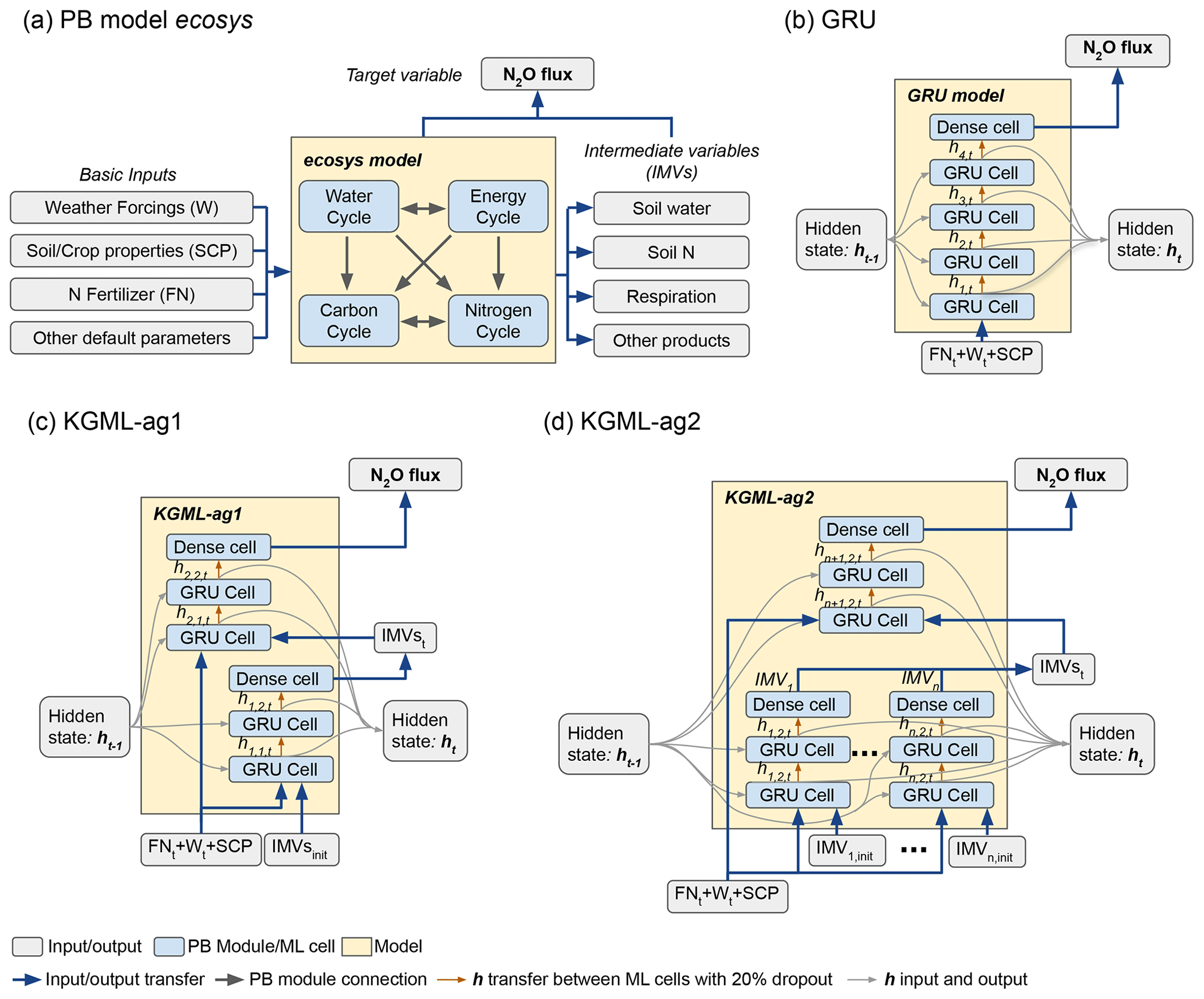
Figure 1 The model structures. (a) The ecosys model; (b) gated recurrent unit (GRU) model; (c) KGML-ag1 model with a hierarchical structure; (d) KGML-ag2 model with a hierarchical structure with separated GRU modules for IMV predictions. Specifically, in our KGML model design, weather forcings (W) include temperature (TMAX, TDIF), precipitation (PRECN), radiation (RADN), humidity (HMAX and HDIF) and wind speed (WIND); soil/crop properties (SCP) include bulk density (TBKDS), sand content (TCSAND), silt content (TCSILT), pH (TPH), cation exchange capacity (TCEC), soil organic carbon (TSOC), planting day of the year (PDOY) and crop type (CROPT); IMVs include CO₂ flux, soil ${{\mathrm{NO}}_{\mathrm{3}}}^{-}$ concentration, soil ${{\mathrm{NH}}_{\mathrm{4}}}^{+}$ concentration and soil volumetric water content (VWC).

2.2.2 Mesocosm experiments for KGML-ag model fine-tuning and evaluation

Observations were acquired from a controlled-environment mesocosm facility on the St. Paul campus of the University of Minnesota. Soil samples were sourced in 2015 from a farm in Goodhue County, MN (44.2339^∘ N, 92.8976^∘ W), which had been under corn–soybean rotation for 25 years. Six chambers with a soil surface area of 2 m² and column depth of 1.1 m were used to plant continuous corn during 2015–2018 and monitor the N₂O flux response to different precipitation treatments. The experiment also measured other environmental variables including air temperature and photosynthetically active radiation (PAR), which were controlled to mimic the outdoor ambient environment. Granular urea fertilizer was hand broadcasted and incorporated to a depth of 0.05 m to each chamber at a rate of 22.4 g N m⁻² (200 lb N ac⁻¹) on 1 May 2015, 4 May 2016 and 3 May 2017, and 10.3 g N m⁻² (92 lb N ac⁻¹) on 8 May 2018. Corn hybrids (DKC-53-56RIB) were hand planted to a depth of 0.05 m in two rows spaced 0.76 m apart 3–5 d after fertilizer application, at a seeding rate of 35 000 seeds ac⁻¹ in 2015 to 2017 and 70 000 seeds ac⁻¹ in 2018 but thinned upon emergence to ensure 100 % emergence at 35 000 seeds ac⁻¹. Crops were harvested at the end of September by cutting the stover five inches above the soil. Hourly N₂O fluxes ($\mathrm{mg}\mathrm{N}{\mathrm{m}}^{-\mathrm{2}}{\mathrm{h}}^{-\mathrm{1}}$) and CO₂ fluxes ($\mathrm{g}\mathrm{C}{\mathrm{m}}^{-\mathrm{2}}{\mathrm{h}}^{-\mathrm{1}}$) were measured using non-steady-state flux chambers with a CO₂ analyzer (LI-10820 for 2016 and LI-7000 for 2017 and 2018, LI-COR Biosciences, Lincoln, NE) and a N₂O analyzer (Teledyne M320EU, Teledyne Technologies International Corp, Thousand Oaks, CA) (a detail method can be retrieved from Fassbinder et al., 2012, 2013). We also collected soil moisture at 15 cm depth (VWC as abbreviation of volumetric water content, m³ m⁻³), weekly 0–15 cm depth soil ${{\mathrm{NO}}_{\mathrm{3}}}^{-}+{{\mathrm{NO}}_{\mathrm{2}}}^{-}$ concentration (${{\mathrm{NO}}_{\mathrm{3}}}^{-}$ for short in the following text, g N Mg⁻¹), soil ${{\mathrm{NH}}_{\mathrm{4}}}^{+}$ concentration (${{\mathrm{NH}}_{\mathrm{4}}}^{+}$, g N Mg⁻¹) and related environment variables including air temperature, radiation, humidity, and soil and crop properties from three growing seasons during 2016–2018 and six mesocosm chambers (Fig. S1 in the Supplement). The magnitude of N₂O flux and ${{\mathrm{NO}}_{\mathrm{3}}}^{-}$ soil concentration and their responses following fertilizer application from this mesocosm experiment are slightly higher than several field studies of agricultural soils (Fassbinder et al., 2013; Grant et al., 1999, 2006, 2008, 2016; Hamrani et al., 2020; Venterea et al., 2011). More details about the mesocosm facility and experimental design can be found in the thesis of Miller (2021).

The observed data were then processed to fine-tune and evaluate the KGML-ag models. The N₂O flux and four IMVs and weather variables were collected from the measurements in the selected period (i.e., 1 April to 31 July). Weekly ${{\mathrm{NO}}_{\mathrm{3}}}^{-}$ (short for soil ${{\mathrm{NO}}_{\mathrm{3}}}^{-}$ within 0–15 cm depth) and ${{\mathrm{NH}}_{\mathrm{4}}}^{+}$ (short for soil ${{\mathrm{NH}}_{\mathrm{4}}}^{+}$ within 0–15 cm) were linearly interpolated to the daily timescale on days containing VWC (short for soil VWC in 15 cm) data. Hourly air temperature, net radiation, N₂O (short for N₂O fluxes from soil), CO₂ (short for CO₂ fluxes from soil) and VWC were resampled to daily scale. All SCPs were derived from mesocosm measurements except that TCEC was derived from the SSURGO database according to the soil origin. We used the leave-one-out cross-validation (LOOCV) method for the evaluation process. Each time, we used five chambers' data for model fine-tuning and one other chamber's data for validation. For example, if we used chambers 1–5 to train the model, then chamber 6 would serve as the out-of-sample data to validate the results. Only the validation results would be presented in our study.

To reduce overfitting and increase the generalization of the trained model based on the small number of mesocosm data, we applied the following method to augment the experimental measurements and weather forcings by a factor of 1000 by sampling hourly data and averaging them to daily scale. In this method, 16 h (or maximum valid hours) of data are randomly selected from 24 h of data to compute their mean as the daily value. Since up to two-thirds of the day is covered by the selected data ($\mathrm{16}\mathrm{h}/\mathrm{24}$ h), the augmented daily values should be representative enough for the source day with slight variations from each other. Furthermore, the observation ratio, $(\mathrm{24}\mathrm{h}-\text{missing hours})/\mathrm{24}\mathrm{h}$, can be used as the weights in loss function to inject the data quality information in model optimization. If the day has more than 16 h missing values, we consider the observations in that day as not trustworthy and drop the day by setting the weight to 0. This method can not only augment the data by a factor of 1000 but also deal with the missing values in observed data inherently. The total number of observed mesocosm data and related weather forcings are augmented to 122 d × 3 years × 6 chambers × 1000 data samples in this study.

2.2.3 Gated recurrent unit as the basis of KGML-ag

Hamrani et al. (2020) compared different models and reported that LSTM provided the highest accuracy in predicting N₂O fluxes because N₂O flux is time-dependent by its production and consumption nature, and LSTM simulates target variables by considering both current and historical states. The LSTM model, proposed by Hochreiter and Schmidhuber (1997), uses a cell state as an internal memory to preserve the historical information. At each time step, it creates a set of gating variables to filter the input and historical information and then uses the processed data to update the cell state. Similar to LSTM, GRU is a gated recurrent neural network but only keeps one hidden state (Cho et al., 2014). Though it is simpler than LSTM, GRU is proven to have similar performance (Chung et al., 2014). Our preliminary test on synthetic data for N₂O prediction showed that GRU indeed provided similar or higher accuracy and model efficiency under different model settings than LSTM (Table S2 in the Supplement). This is possible because simpler models with fewer weights and hyperparameters are more robust in combating the overfitting problem. Therefore, we choose GRU as the basis of KGML-ag development.

2.2.4 Incorporating domain knowledge to the development of KGML-ag

To quantitatively reveal the correlations between N₂O fluxes and IMVs and guide the KGML-ag development, we conducted feature importance analysis by a customized four-layer GRU ML model (Fig. 1b). Each layer of the model has a GRU cell with 64 hidden units. The four-layer structure makes the model deeper and capable of capturing complex interactions. Between each GRU cell, 20 % of the output hidden states are randomly dropped by replacing them with zero values (the so-called 20 % dropout) to avoid overfitting. A dense linear layer is used to map the final output to N₂O. We first trained GRU models using synthetic data with different combinations of IMVs as inputs to predict the N₂O fluxes (original test, Table S2). The feature importance analysis of well-trained models was then implemented by replacing one input feature with a Gaussian noise with mean μ=0 and standard deviation σ=0.01, while keeping others untouched (new test). The importance score was calculated by the new test's root mean square error (RMSE) (replacing one feature) minus the original test's RMSE (no replacing). RMSE was calculated by $\sqrt{{\sum }_{\mathrm{1}}^N(y_i-y_i^{\prime }{)}^{\mathrm{2}}}/N$, where N is the total number of observations across time and space, y_i is the ith measurement from synthetic data or observed data and $y_i^{\prime }$ is its corresponding prediction.

To find important variables for N₂O flux prediction in an ideal situation where all variables are available, we conducted a feature importance analysis for GRU models with all IMVs and basic inputs including FN, 7W and 8SCP (Fig. S2a). Results indicated that flux variables including NH₃, H₂, N₂, O₂, CH₄, evapotranspiration (ET) and CO₂ had significant influence on the model performance. Variables ranked high in feature importance analysis are considered with priority during model development. To develop a functional KGML-ag, we further investigated the feature importance of four IMVs that are available from mesocosm observations including CO₂, ${{\mathrm{NO}}_{\mathrm{3}}}^{-}$, VWC and ${{\mathrm{NH}}_{\mathrm{4}}}^{+}$, which were ranked 7th, 20th, 58th, 60th respectively in 92 input features of synthetic data (Fig. S2a). We used these four available IMVs to create two input combinations: (1) CO₂ flux, ${{\mathrm{NO}}_{\mathrm{3}}}^{-}$, VWC and ${{\mathrm{NH}}_{\mathrm{4}}}^{+}$ (IMVcb1), and (2) ${{\mathrm{NO}}_{\mathrm{3}}}^{-}$, VWC and ${{\mathrm{NH}}_{\mathrm{4}}}^{+}$ (IMVcb2). The objective of building IMVcb2 was to investigate the importance of the highly ranked variable CO₂ flux (by removing it from the inputs) and the impact of mixing up flux and non-flux variables on model performance. We tested the feature importance of the GRU models built with IMVcb1 and IMVcb2 to check whether they would help in N₂O prediction (Fig. S2b and c). All the feature importance results above indicated the correlation intensity between N₂O and many other variables, which would help the KGML-ag model development and interpretation in this study (rest of this section and Sect. 3.1) and would guide future N₂O-related measurements and KGML model development (discussed in Sect. 4.3).

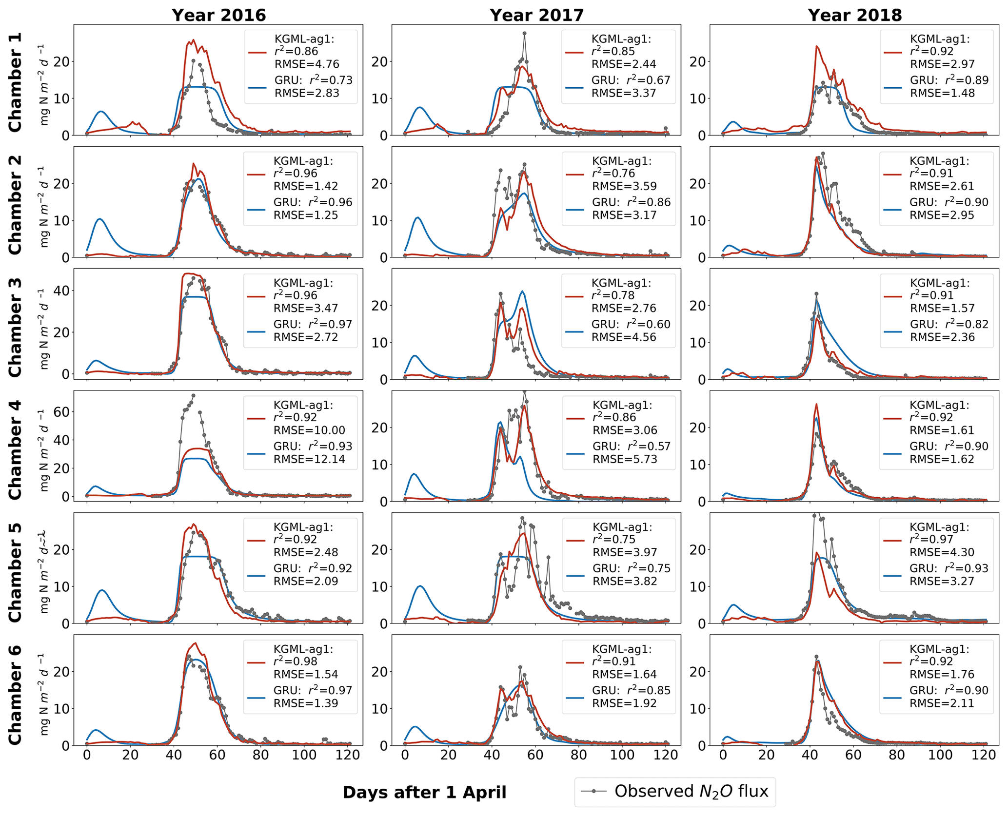
Figure 2 Leave-one-out cross validation of time series of N₂O flux ($\mathrm{mg}\mathrm{N}{\mathrm{m}}^{-\mathrm{2}}{\mathrm{d}}^{-\mathrm{1}}$) predicted by the pure non-pre-trained GRU model (blue line) and KGML-ag1 model (red line). Observations are shown as black line dots. Validation results for each chamber were based on out-of-sample predictions by models trained by the other five chambers.

Next, we used the knowledge learned from synthetic data to develop the structure of KGML-ag (Fig. 1c and d). Previous studies for KGML models have used physical laws, e.g., conservation of mass or energy, to design the loss function for constraining the ML model to produce physically consistent results (Read et al., 2019; Khandelwal et al., 2020). However, for complex systems like agroecosystems, it is challenging to incorporate physical laws, such as mass balance for N₂O, into the loss function due to the incomplete understanding of the processes and the lack of mass-balance-related data for validation. An alternative solution is to incorporate such information in the design of the neural network (Willard et al., 2021). Effectiveness of such an approach was demonstrated by Khandelwal et al. (2020) in the context of modeling stream flow in a river basin using Soil and Water Assessment Tool (SWAT). They used a hierarchical neural network to explicitly model IMVs (e.g., soil moisture, snow cover) and their relationships with the target variable (streamflow) and showed that this model is much more effective than a neural network that attempts to directly learn the relationship between input drivers and the target variables. Following this idea, we identified four desired features of an effective KGML-ag model, including the following. (1) We used initial values instead of sequence of the IMVs from synthetic data or observed data to provide a solid starting state for the ML system and reduce the IMV data demand and then used the rest of the data to further constrain the prediction of IMVs. (2) We built a hierarchical structure based on the structure of process representation in ecosys to first predict IMVs and then simulate N₂O with predicted IMVs. (3) We trained all variables together using multi-task learning to reach the best prediction scores, which generalized the model and incorporated interactions between IMVs and N₂O. (4) We initialized the KGML-ag model by pre-training with synthetic data before using real observed data to transfer physical knowledge, which further reduced the demand on large training samples and aided in faster convergence for fine-tuning.

To meet these desired features, we proposed two KGML-ag models (Fig. 1c and d). The first model, KGML-ag1, is a hierarchical structure containing two modules to simulate IMVs and N₂O sequentially. Each module is a 2-layer 64 units GRU ML model. The inputs to the module of the KGML-ag1 model for IMV predictions (KGML-ag1-IMV module) are FN, 7W and 8SCP together with the initial values of IMVs, and the outputs are IMV predictions. The inputs to the module of the KGML-ag1 model for N₂O predictions (KGML-ag1-N₂O module) are FN, 7W, 8SCP and predicted IMVs from KGML-ag1-IMV, and the output is the target variable N₂O. Linear dense layers were coded for both modules to map output states to IMVs or N₂O. The dropout method was applied to drop 20 % of the state output between GRU cells and dense layers. The second model, KGML-ag2, is also a hierarchical structure similar to KGML-ag1, but has multiple KGML-ag2-IMV modules to explicitly simulate IMVs by tuning them separately in the fine-tuning process (discussed in Sect. 2.2.5). Each KGML-ag2-IMV module in KGML-ag2 is a two-layer 64 units GRU cell with the inputs of FN, 7W, 8SCP and one IMV initial value and the output of one IMV prediction. The KGML-ag2-N₂O module collects the IMV predictions from KGML-ag2-IMV modules and predicts the N₂O with inputs of FN, 7W and 8SCP and predicted IMVs.

2.2.5 Strategies for pre-training and fine-tuning processes

To increase the efficiency of the training process, we used the Z-normalization ($(X-\mathit{\mu })/\mathit{\sigma }$, where X is the vector of a particular variable over all the data samples in the dataset; μ is the mean value of X; σ is the standard deviation of X) method to normalize each variable separately on synthetic data. Then the scaling factors (μ, σ) derived from ecosys synthetic data for each variable were used to ​​​​​​​normalize observed data into the same ranges as synthetic data. As mentioned in Sect. 2.2.1, the TDIF_AIR, HDIF_AIR were used instead of absolute min temperature (TMIN_AIR) and humidity (HMIN_AIR). This is done because TMIN_AIR and HMIN_AIR follow similar trends as TMAX_AIR and HMAX_AIR, making Z-normalization numerically poorly defined. Using the difference between maximum and minimum can provide a clearer information of daily air temperature and humidity variation.

During the pre-training process, we initialized the IMV of KGML-ag using the first day value of synthetic IMV time series. Adam optimizer with a start learning rate of 0.0001 was used for the training process. The learning rate would decay by 0.5 times after every 600 training epochs. At each epoch, synthetic data samples were randomly shuffled before being input to the model to predict N₂O (and IMVs if any). The mean square error (MSE) loss (calculation was equal to the square of RMSE) or sum of MSE loss (if multi-task learning) between predictions and ecosys synthetic observations were calculated to optimize the weights of GRU cells. After the training process updated the model's weights, the validation process was performed to evaluate the model performance based on untouched samples with RMSE and the square of Pearson correlation coefficient (r²). The r² was calculated as $\left({\sum }_i\right(y_i^{\prime }-\underset{\mathrm{¯}}{y_i^{\prime }}\left)\right(y_i-\underset{\mathrm{¯}}{y_i}){)}^{\mathrm{2}}/({\sum }_i(y_i^{\prime }-\underset{\mathrm{¯}}{y_i^{\prime }}{)}^{\mathrm{2}}(y_i-\underset{\mathrm{¯}}{y_i}{)}^{\mathrm{2}})$, where y_i is the ith measurement from synthetic data or observed data, $y_i^{\prime }$ is its corresponding prediction, $\underset{\mathrm{¯}}{y_i}$ is the mean of the measurement y in diagnosing space and $\underset{\mathrm{¯}}{y_i^{\prime }}$ is the mean of the predicted y^′ in diagnosing space. If both validated r² and RMSE were better than the best values in previous epochs, the updated model in this epoch would be saved. Normalized RMSE (NRMSE, calculated by RMSE$/$(max–min) of each variable observation) was introduced to evaluate IMV predictions between variables with different value ranges.

During the fine-tuning process, we used estimated IMV initial values of 1.0 g C m⁻², 0.2 m³ m⁻³, 0.0 g N Mg⁻¹ and 20.0 g N Mg⁻¹ for CO₂, VWC, ${{\mathrm{NH}}_{\mathrm{4}}}^{+}$ and ${{\mathrm{NO}}_{\mathrm{3}}}^{-}$ respectively, from starting day (1 April) to the day before the first day of real observations, as input to KGML-ag models. Then the first-day values of observed IMVs were input into KGML-ag during the rest of the days of the period as IMV initial values. In addition, as described in Sect. 2.2.2, we used a data augmentation method to augment the total number of data by a factor of 1000 for the fine-tuning process. The purpose of this data augmentation method was to increase the generalization of the fine-tuned model and to overcome the overfitting due to small sample size. The mask matrix was elementarily multiplied to the output matrix to calculate the MSE, r² and RMSE only for days with observations. The similar optimizer was used with an initial learning rate of 0.00005 and decay fraction of 0.5 per 200 epochs. Other training and validation methods in each epoch were similar to the pre-training process. Specifically, in the KGML-ag1 model fine-tuning process, we first froze the KGML-ag1-N₂O module and only trained the KGML-ag1-IMV module for IMVs. After finishing the KGML-ag1-IMV module training, we froze the KGML-ag1-IMV module and trained the KGML-ag1-N₂O module for N₂O. In the KGML-ag2 fine-tuning process, the similar freezing method was used but different KGML-ag2-IMV modules were trained separately one by one.

2.3 Development environment description

We used the Pytorch 1.6.0 (https://pytorch.org/get-started/previous-versions/, last access: 15 September 2021) and Python 3.7.9 (https://www.python.org/downloads/release/python-379/, last access: 15 September 2021) as the programming environment for the model development. In order to use the GPU to speed-up the training process, we installed CUDA Toolkit 10.2.89 (https://developer.nvidia.com/cuda-toolkit, last access: 15 September 2021). A desktop with NVIDIA 2080 super GPU was used for code development and testing. The Mangi cluster (https://www.msi.umn.edu/mangi, last access: 15 September 2021) from High-Performance Computing of Minnesota Supercomputing Institute (HPC-MSI, https://www.msi.umn.edu/content/hpc, last access: 15 September 2021) with two-way NVIDIA Tesla V100 GPU was used in training processes which consumed longer time and bigger memory space.

3 Results

3.1 Pre-training experiments using synthetic data from ecosys

In the pre-training stage, the GRU model with 76 IMVs achieved the best performance in predicting N₂O fluxes (r²=0.98, RMSE=0.54 $\mathrm{mg}\mathrm{N}{\mathrm{m}}^{-\mathrm{2}}{\mathrm{d}}^{-\mathrm{1}}$ and normalized RMSE (NRMSE)=0.01) on the test set of synthetic data generated from ecosys (Table 1). The high performance was due to some flux IMVs such as NH₃, H₂, O₂, CO₂ and ET, which are highly correlated to N₂O (Fig. S2a), were used as input to the model. The good performance of GRU with all IMVs indicates that ML models are able to perfectly mimic ecosys when sufficient information about IMVs is available. The GRU model with only basic input of N fertilizer rate, seven weather forcings, and eight soil and crop properties (FN, 7W and 8SCP) had the accuracy of r²=0.89 and RMSE=1.37 $\mathrm{mg}\mathrm{N}{\mathrm{m}}^{-\mathrm{2}}{\mathrm{d}}^{-\mathrm{1}}$ (Table 1). The relatively low performance is likely because this model failed to capture several highly nonlinear pathways that are employed by ecosys to predict N₂O (e.g., one influence pathway from precipitation to N₂O can be precipitation → soil moisture → N component solubility and concentration → nitrification and denitrification rate and amount → soil N₂O concentration → gas N₂O flux). When adding sequences of IMV combinations (i.e., IMVcb1 of CO₂ flux, ${{\mathrm{NO}}_{\mathrm{3}}}^{-}$, ${{\mathrm{NH}}_{\mathrm{4}}}^{+}$ and VWC, and IMVcb2 of ${{\mathrm{NO}}_{\mathrm{3}}}^{-}$, ${{\mathrm{NH}}_{\mathrm{4}}}^{+}$ and VWC), the GRU models performed slightly better than the GRU model using only basic inputs, achieving r² of 0.92 and 0.90, respectively (Table 1). The KGML-ag1 with IMVcb1 and IMVcb2 initial values provided better performance (both r²=0.90) than GRU with basic input and comparable performance to the GRU with inputs of IMVcb1 and IMVcb2 sequence. Besides, KGML-ag1 provided predicted IMVs of CO₂, ${{\mathrm{NO}}_{\mathrm{3}}}^{-}$, ${{\mathrm{NH}}_{\mathrm{4}}}^{+}$ and VWC with r² over 0.91 and NRMSE below 0.06 (Table 1). KGML-ag2 also provided comparable N₂O performance but relatively better IMV performance of r² over 0.92 and NRMSE below 0.05. Results indicated that KGML-ag models with IMV initial values as extra input performed similar or better than pure ML models in synthetic data.

Table 1 Pre-train results for different model and IMV combinations using ecosys synthetic data. Only the performance from testing datasets (synthetic data from 19 counties) was presented.

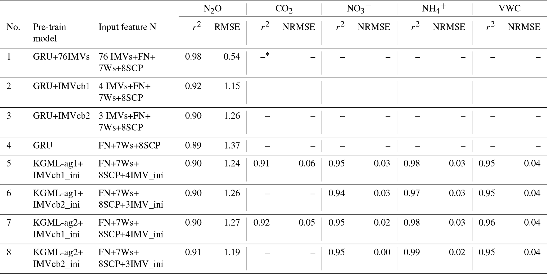
^* The empty slot indicates that the model does not predict that variable.

3.2 KGML-ag evaluation using observed data from mesocosm

After being fine-tuned with observed data, KGML-ag1 had N₂O prediction overall accuracy of r²=0.81 and RMSE=3.6 $\mathrm{mg}\mathrm{N}{\mathrm{m}}^{-\mathrm{2}}{\mathrm{d}}^{-\mathrm{1}}$, while the non-pre-trained GRU model provided r²=0.78 and RMSE=4.0 $\mathrm{mg}\mathrm{N}{\mathrm{m}}^{-\mathrm{2}}{\mathrm{d}}^{-\mathrm{1}}$, and the pre-trained GRU model provided r²=0.80 and RMSE=3.77 $\mathrm{mg}\mathrm{N}{\mathrm{m}}^{-\mathrm{2}}{\mathrm{d}}^{-\mathrm{1}}$ (Table 3). The time series of N₂O predictions from KGML-ag1 and the non-pre-trained GRU model were further compared (Fig. 2), from which we found at least two advantages of using KGML-ag1 for N₂O predictions. (1) For the region without observation data (normally before day 25), KGML-ag1 predicted stable N₂O fluxes close to 0 $\mathrm{mg}\mathrm{N}{\mathrm{m}}^{-\mathrm{2}}{\mathrm{d}}^{-\mathrm{1}}$ (which is close to the reality in the experiment setting), while GRU caused anomalous peaks of fluxes. This is because KGML-ag1 has learned knowledge for the whole period from the pre-training process with ecosys model-generated synthetic data, but the GRU model has no prior knowledge for the period without any data in observations. (2) Although KGML-ag1 had a lower accuracy than GRU in some chambers, KGML-ag1 can better capture the temporal dynamics of N₂O fluxes compare to GRU, especially when the fluxes are highly variable (e.g., Fig. 2, chamber 2).

Table 2 Prediction accuracy comparisons between non-pre-trained GRU model and KGML-ag1.

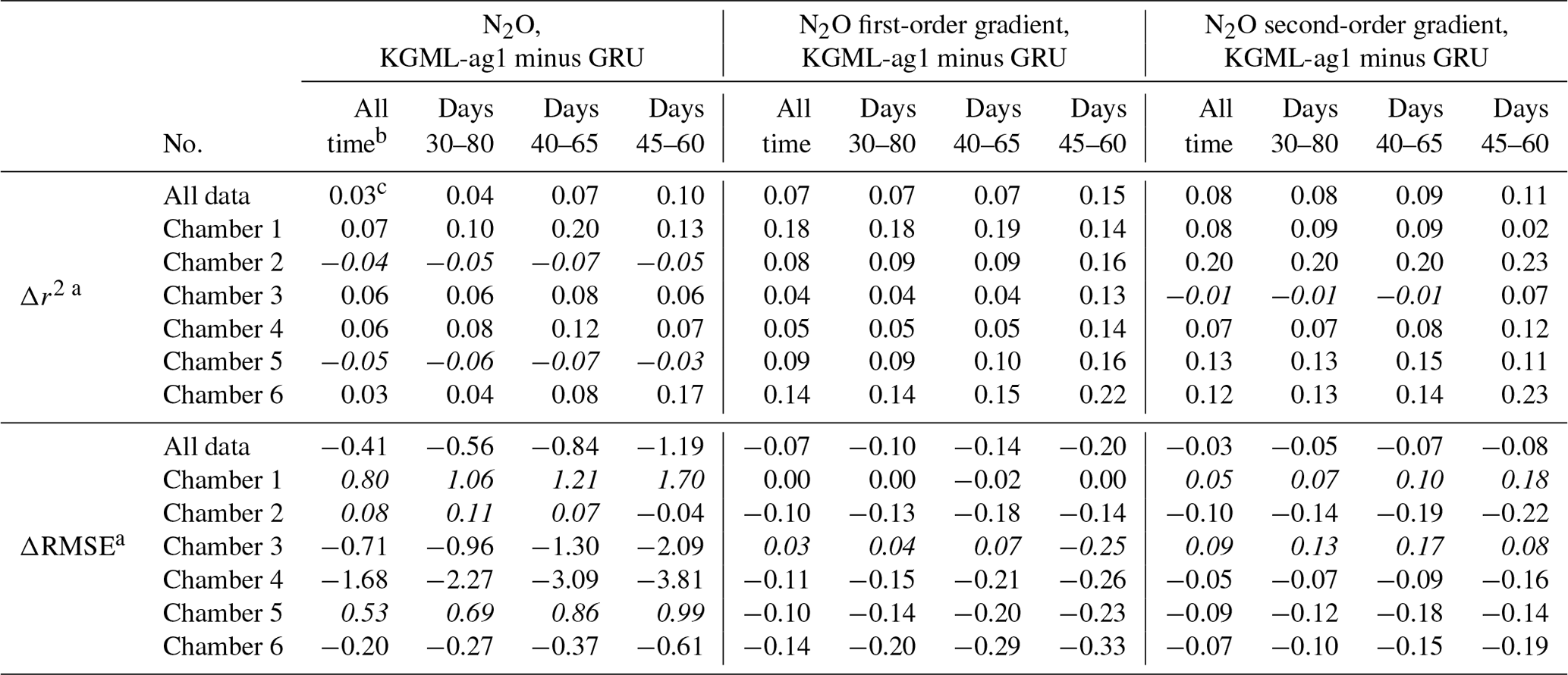
^a Leave-one-out cross validation results for each chamber were based on out-of-sample predictions by models trained by other five chambers. The “all data” performance was calculated by comparing out-of-sample predictions from all validated chambers with observations. The difference of r² (Δr²) and difference of RMSE (ΔRMSE; units are $\mathrm{mg}\mathrm{N}{\mathrm{m}}^{-\mathrm{2}}{\mathrm{d}}^{-\mathrm{1}}$, $\mathrm{mg}\mathrm{N}{\mathrm{m}}^{-\mathrm{2}}{\mathrm{d}}^{-\mathrm{2}}$, $\mathrm{mg}\mathrm{N}{\mathrm{m}}^{-\mathrm{2}}{\mathrm{d}}^{-\mathrm{3}}$ for N₂O value, first-order gradient and second-order gradient, respectively) were calculated by values from KGML-ag1 minus values from GRU. ^b Results from different time windows of different chambers during the period of 1 April–31 July (days 1–122) were detected. ^c The values not in italics mean KGML-ag1 outperforms GRU, while values in italics mean the opposite.

Table 3 Experiments for measuring GRU and KGML-ag model performance and the influence of pre-training process, training data augmentation and IMV initial values.

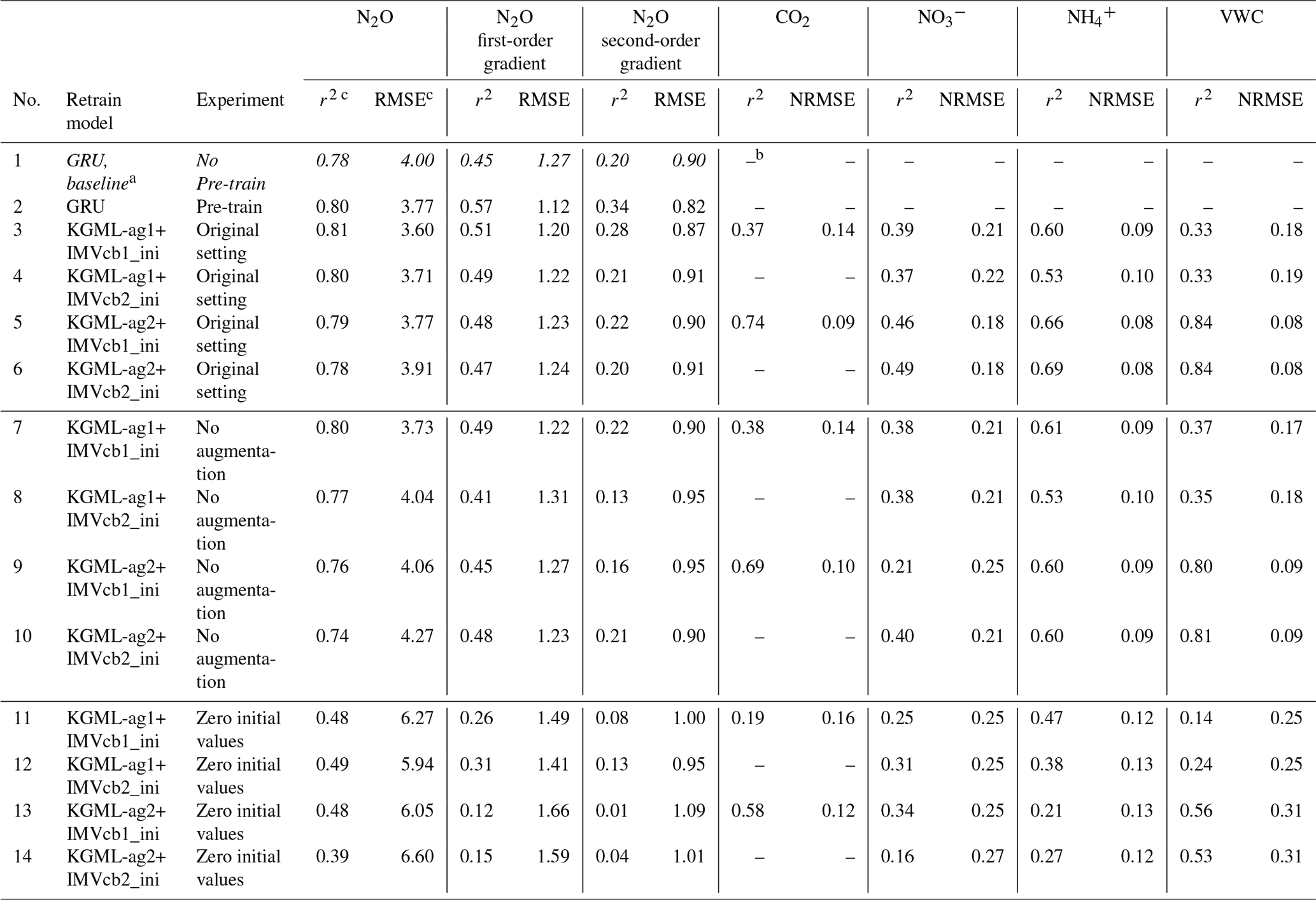
^a Nos. 1–6 include the experiments with original simulation settings as described in Sect. 2, and values in italics refer to the baseline GRU simulation; nos. 7–10 include the experiments without data augmentation during the fine-tuning process; and nos. 11–14 include the experiments of replacing original IMV initial values with zeros. ^b The empty slot indicates that the model does not predict that variable. ^c The leave-one-out cross-validation overall performance was calculated by comparing out-of-sample predictions (each chamber's predictions were from models trained by other five chambers) from all validated chambers with observations.

To validate KGML-ag1 robustness, we further investigated the KGML-ag1 and GRU model performance in different temporal windows, shrinking from the whole period to the N₂O peak occurrence time (days 1–122, days 30–80, days 40–65 and days 45–60 for the years 2016–2018) and performance in N₂O flux, first-order gradient of N₂O (slope) and second-order gradient of the N₂O (curvature) (Table 2). Slope represents the speed of N₂O flux changes through time and curvature represents the acceleration. Assessing prediction performance with these two metrics will reveal the model robustness on capture variable dynamics, which is critical when predicting fast-change variables with hot moments (a short period of time with rare events like flux increasing quickly) like N₂O. First of all, the overall r² and RMSE of KGML-ag1 for values, slope and curvature were always better than GRU. In particular, KGML-ag1 captured the peak region (e.g., days 45–60) much better than GRU in both magnitude and dynamics (Table 2 and Fig. 2). Even for chambers 2 and 5 in which KGML-ag1 made worse N₂O predictions than GRU (Δr² ranging from −0.07 to −0.03), it better captured temporal dynamics than GRU in terms of slope (Δr² ranging from 0.08 to 0.16) and curvature (Δr² from 0.11 to 0.23) (Table 2). For other chambers, KGML-ag1 outperformed GRU consistently. For chamber 1, KGML-ag1 had worse N₂O predictions RMSE than GRU but the Δr² increased as the window shrinks to the peak emission time (0.07→0.13). The slope and curvature for chamber 1 also indicated that KGML-ag1 captured the dynamics much better than GRU. For chamber 3, KGML-ag1 predicted better N₂O but presented worse slope and curvature RMSE than GRU (Table 2). However, when explicitly investigating the time series of N₂O flux, slope and curvature in each year, KGML-ag1 outperformed GRU more significantly in 2017, the year with more complex temporal dynamics of N₂O fluxes, than in 2016 and 2018, especially for chamber 3 (Figs. 2, S3 and S4). This investigation supported that KGML-ag1 was more capable for complex dynamics predictions.

Interestingly, the fine-tuned KGML-ag1 model predicted reasonable IMVs including CO₂, ${{\mathrm{NO}}_{\mathrm{3}}}^{-}$, ${{\mathrm{NH}}_{\mathrm{4}}}^{+}$ and VWC with overall r² of 0.37, 0.39, 0.60 and 0.33 and NRMSE of 0.14, 0.21, 0.09 and 0.18, respectively (Table 3). The time series comparisons between IMV predictions and observations further indicated that KGML-ag1 could reasonably capture both magnitude and dynamics (Fig. 3). KGML-ag2 presented better IMV predictions than KGML-ag1, with overall r² of CO₂, ${{\mathrm{NO}}_{\mathrm{3}}}^{-}$, ${{\mathrm{NH}}_{\mathrm{4}}}^{+}$ and VWC increasing by 0.37, 0.17, 0.06 and 0.51, and NRMSE decreasing by 0.05, 0.03, 0.01 and 0.10, respectively, but a slightly lower r² (decreasing 0.02) of N₂O (Table 3 and Fig. S5). This indicated that explicitly simulating each IMV with separated KGML-ag2-IMV modules did not benefit the N₂O flux prediction accuracy, likely due to increasing model complexity which resulted in reduced stability and ignoring the IMV interactions. In addition, we also found all KGML-ag models would perform better by using IMVcb1 (with CO₂) than using IMVcb2 (without CO₂) in real data tests, indicating feature importance analysis based on synthetic data can be a reasonable substitute for analysis with the often limited real-world data.

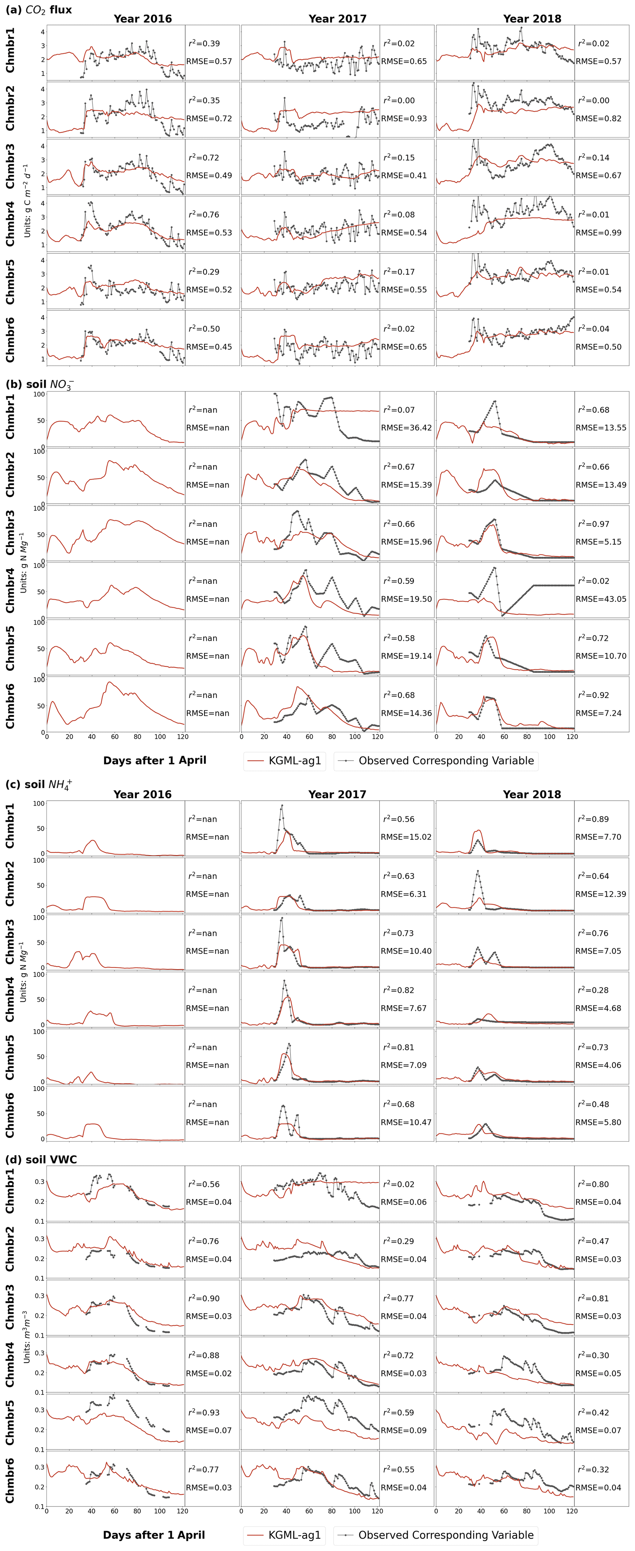
Figure 3 Leave-one-out cross validation of time series of IMVs predicted by KGML-ag1 model (red line). Observations are shown as black line-dots. Validation results for each chamber were based on out-of-sample predictions by models trained by other five chambers. Chmb is the abbreviation for chamber. r² and RMSE are calculated and present in each year and chamber. The CO₂ flux (a) and soil ${{\mathrm{NO}}_{\mathrm{3}}}^{-}$ concentration (b) units are $\mathrm{g}\mathrm{C}{\mathrm{m}}^{-\mathrm{2}}{\mathrm{d}}^{-\mathrm{1}}$ and g N Mg⁻¹, respectively. The soil ${{\mathrm{NH}}_{\mathrm{4}}}^{+}$ concentration (c) and soil VWC (d) units are g N Mg⁻¹ and m³ m⁻³, respectively.

3.3 KGML-ag comparing with other pure ML models

The results from eight different models showed that KGML-ag1 comparing with other pure ML models consistently provided the lowest RMSE (3.59–3.94 $\mathrm{mg}\mathrm{N}{\mathrm{m}}^{-\mathrm{2}}{\mathrm{d}}^{-\mathrm{1}}$, 1.14–1.23 $\mathrm{mg}\mathrm{N}{\mathrm{m}}^{-\mathrm{2}}{\mathrm{d}}^{-\mathrm{2}}$ and 0.84–0.89 $\mathrm{mg}\mathrm{N}{\mathrm{m}}^{-\mathrm{2}}{\mathrm{d}}^{-\mathrm{3}}$) and highest r² (0.78–0.81, 0.48–0.56 and 0.23–0.31) for N₂O fluxes, slope and curvature, respectively (Fig. 4). This indicated that KGML-ag1 outperformed other pure ML models in capturing both the magnitude and dynamics of N₂O flux. Meanwhile, we have calculated the uncertainty of mesocosm measurement due to converting hourly data to daily data during 30–80 d by using augmented values minus the mean of the augmented values with lower and upper limits being −10.2 and 10.4 $\mathrm{mg}\mathrm{N}{\mathrm{m}}^{-\mathrm{2}}{\mathrm{d}}^{-\mathrm{1}}$, respectively (standard deviation = 1.4 $\mathrm{mg}\mathrm{N}{\mathrm{m}}^{-\mathrm{2}}{\mathrm{d}}^{-\mathrm{1}}$). KGML-ag1 during the same period has comparable uncertainties based on ensemble simulations with lower and upper limits being −14.4 and 15.2 $\mathrm{mg}\mathrm{N}{\mathrm{m}}^{-\mathrm{2}}{\mathrm{d}}^{-\mathrm{1}}$, respectively (calculated by ensemble values minus the mean of ensemble values; standard deviation of 1.3 $\mathrm{mg}\mathrm{N}{\mathrm{m}}^{-\mathrm{2}}{\mathrm{d}}^{-\mathrm{1}}$). KGML-ag2 presented slightly better mean scores for N₂O flux predictions than KGML-ag1, but worse scores for slope and curvature and larger uncertainties. This proved the hypothesis discussed in Sect. 3.2 that KGML-ag2 did not benefit the magnitude and dynamics predictions of N₂O flux with its more complex structure and less connections between IMVs.

Figure 4 The comparisons of overall prediction accuracy from leave-one-out cross validation for N₂O value (a), first-order gradient (slope, b) and second-order gradient (curvature, c) between four tree-based ML models (DT, RF, GB and XGB), two deep-learning models (ANN and GRU) and KGML-ag models. The overall performance was calculated by comparing out-of-sample predictions (each chamber's predictions were from models trained by other five chambers) from all validated chambers with observations. Different color symbols represent the different models. The x- and y-error bars are coming from the maximum and minimum scores of ensemble experiments. The dot represents the mean score of the ensemble experiments.

Within the tree-based models (DT, RF, GB and XGB), the simplest model DT provided the worst predictions for N₂O flux, slope and curvature. The XGB model provided the highest N₂O flux accuracy with r² of 0.61–0.63 and RMSE of 5.07–5.17 $\mathrm{mg}\mathrm{N}{\mathrm{m}}^{-\mathrm{2}}{\mathrm{d}}^{-\mathrm{1}}$, while the GB model provided best slope and curvature predictions with r² of 0.38–0.40 and 0.23–0.26, and RMSE of 1.34–1.37 $\mathrm{mg}\mathrm{N}{\mathrm{m}}^{-\mathrm{2}}{\mathrm{d}}^{-\mathrm{2}}$ and 0.91–0.95 $\mathrm{mg}\mathrm{N}{\mathrm{m}}^{-\mathrm{2}}{\mathrm{d}}^{-\mathrm{3}}$, respectively. The highest N₂O flux accuracy and relatively low slope and curvature accuracy of the XGB model implied that there is a trade-off between the abilities of capturing dynamics and magnitude.

In the group of deep-learning models including ANN, GRU and KGML-ag1, ANN provided the worst predictions. Even with the better N₂O flux predictions than most tree-based models (except XGB), the slope and curvature predictions of ANN were the worst among all eight models. This implied that the trade-off between accurately capturing N₂O dynamics to magnitude in ANN was significant. But when considering the temporal dependence, deep-learning models GRU and KGML-ag1 outperformed all other models in flux, slope and curvature predictions. This indicated that without considering temporal dependence the improvement in N₂O flux prediction accuracy could be risky by causing the performance drop in capturing dynamics.

The detailed model comparisons in each chamber are shown in Fig. 5 (N₂O flux) and Figs. S6 and S7 (N₂O slope and curvature), where the results are found to follow the same pattern as described above. In addition, time series comparisons of chambers 3 and 4 in 2017 between different models are presented in Fig. S8 as two examples. For periods without any observed data, we assumed that the good model predictions should be stable, consistent with the nearest period and close to the reality in the experiment setting (e.g., no erratic peak and N₂O flux near 0 $\mathrm{mg}\mathrm{N}{\mathrm{m}}^{-\mathrm{2}}{\mathrm{d}}^{-\mathrm{1}}$ before day 25). From these comparisons, we infer that without considering temporal dependence and pre-training process, the tree-based model including DT, RF, GB and XGB and deep-learning model ANN predicted erratic peaks in almost every missing data point, while the GRU model was stable in short missing period (1–2 d of missing data) and only presented poor performance in long missing period (before day 25). This improvement by the GRU model may be attributed to the structure of GRU that naturally keeps the historical information using hidden states, which enables GRU to consider the temporal dependence and make consistent predictions over time.

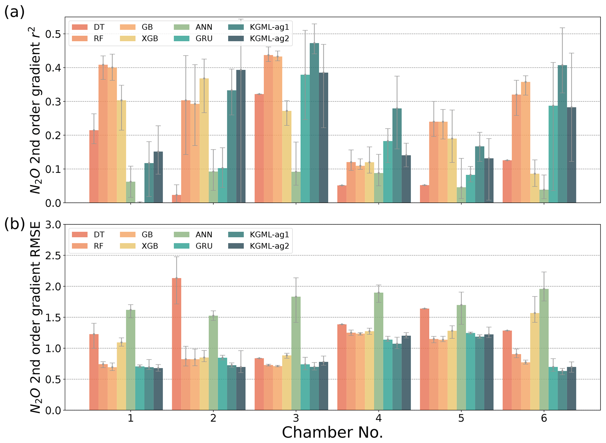
Figure 5 The comparisons of N₂O flux prediction accuracy r² (a) and (b) RMSE from leave-one-out cross validation, between four tree-based ML models (DT, RF, GB and XGB), two deep-learning models (ANN and GRU) and KGML-ag models in six chambers. Validation results for each chamber were based on out-of-sample predictions by models trained by other five chambers. The gray error bars are coming from the maximum and minimum scores of ensemble experiments.

3.4 Influence of pre-training process, data augmentation and using IMV initial values as input feature

After we pre-trained the GRU model with synthetic data, the overall r² of N₂O flux predictions in observed data increased by 0.02, 0.12 and 0.14, and RMSE decreased by 0.23 $\mathrm{mg}\mathrm{N}{\mathrm{m}}^{-\mathrm{2}}{\mathrm{d}}^{-\mathrm{1}}$, 0.15 $\mathrm{mg}\mathrm{N}{\mathrm{m}}^{-\mathrm{2}}{\mathrm{d}}^{-\mathrm{2}}$ and 0.02 $\mathrm{mg}\mathrm{N}{\mathrm{m}}^{-\mathrm{2}}{\mathrm{d}}^{-\mathrm{3}}$ for flux, slope and curvature predictions, respectively, compared to non-pre-trained GRU (nos. 1–6 in Table 3). The gap between the GRU model with pre-train and KGML-ag1 in N₂O value prediction shows the improvement resulting from architecture change (r² increases by 0.01 and RMSE decreases by 0.17 $\mathrm{mg}\mathrm{N}{\mathrm{m}}^{-\mathrm{2}}{\mathrm{d}}^{-\mathrm{1}}$). Although pre-trained GRU had higher slope and curvature prediction accuracy than KGML-ag models, it still could not achieve the current N₂O value prediction accuracy of KGML-ag1. Besides, the KGML-ag models had relatively shallow N₂O prediction modules (two-layer GRU KGML-ag-N₂O module of KGML-ag models vs. four-layer GRU) but included modules for IMV predictions, which therefore increased the model interpretability.

It is worth noting that prediction accuracy of all KGML-ag models dropped without augmenting the training dataset in the fine-tuning process (nos. 7–10 in Table 3). Moreover, the maximum training epochs increased from 800 to 20 000, which resulted in overfitting on the small dataset. This indicated that the data augmentation indeed helped the models become more generalizable and gain better accuracy.

Experiments using zero initial values presented a significant drop in every variable's prediction accuracy (nos. 11–14 in Table 3). This indicated that the IMV initial values input into the KGML-ag-IMV modules of KGML-ag models influenced not only the IMV prediction but also the N₂O prediction of the KGML-ag-N₂O module. This shows that there is useful information transferred from IMVs in the KGML-ag-IMV module to the KGML-ag-N₂O module.

4 Discussion

In the previous section, we showed that KGML-ag models can outperform ML models, by invoking architectural constraints and PB model synthetic data initialization. Compared to traditional PB models such as ecosys, KGML-ag models provide computationally more accurate and efficient predictions (KGML-ag few seconds vs. ecosys half hour), which is similar to traditional ML surrogate models (Fig. S9 in the Supplement). But KGML-ag goes beyond that by providing more interpretable predictions than pure ML models.

4.1 Interpretability of KGML-ag

The proposed KGML-ag models incorporate causal relations among N₂O-related variables and processes as shown in Fig. S10 in the Supplement. Managements, weather forcings and initial values of IMVs influence soil water, soil temperature and soil properties, which influence the availability of O₂ and N as well as the microbe populations in soil and further influence the nitrification and denitrification rates. N₂O is produced during both nitrification and denitrification when soil O₂ concentration is limited. Our KGML-ag follows this hierarchical structure by designing KGML-ag-IMV modules representing the soil processes for IMV predictions (Fig. 1c and d).

To better explain the time series predictions of N₂O flux (Figs. S1, 2 and 3), we separated the observations of each year into three periods: leading period (before N₂O increasing), increasing period (increasing to the peak) and decreasing period (peak decreasing to near zero). During the leading period, both ${{\mathrm{NH}}_{\mathrm{4}}}^{+}$ and CO₂ were increasing immediately in the following few days following urea N fertilizer application, indicating that urea was decomposing into ${{\mathrm{NH}}_{\mathrm{4}}}^{+}$ and CO₂ in soil water. With accumulating ${{\mathrm{NH}}_{\mathrm{4}}}^{+}$ in soil, nitrification started producing ${{\mathrm{NO}}_{\mathrm{3}}}^{-}$ and consuming O₂. N₂O did not respond to the fertilizer immediately due to enough O₂ in soil. Then when the soil became sufficiently hypoxic, N₂O fluxes entered an increasing period with N₂O being produced by nitrification and denitrification processes. CO₂ fluxes were relatively low and ${{\mathrm{NH}}_{\mathrm{4}}}^{+}$ kept decreasing during this period. Finally, when soil ${{\mathrm{NH}}_{\mathrm{4}}}^{+}$ was exhausted and ${{\mathrm{NO}}_{\mathrm{3}}}^{-}$ started decreasing due to denitrification, N₂O fluxes then entered the decreasing period. CO₂ flux was related to urea decomposition during the leading period and was more closely related to O₂ demand in other periods. The KGML-ag predictions of N₂O and IMV captured the three periods and transition points, demonstrating the connections between those variables following the description as above (Figs. 3 and S5). Although KGML-ag1 obtained lower IMV prediction accuracy compared to KGML-ag2, it captured the general trends and was doing better for transitions, especially in ${{\mathrm{NH}}_{\mathrm{4}}}^{+}$ predictions. KGML-ag2 overfitted on the observations and ignored the correlations between IMVs, which resulted in loss in pre-train knowledge, poorer performance in the leading period and erratic predictions in the period with missing observations (before day 25).

4.2 Lessons for KGML-ag development

The development of KGML-ag in our study is suitable to predict not only N₂O but also other variables, such as CO₂, CH₄ and ET, with complicated generation processes relying on the historical states. To develop a capable KGML model, we need to carefully address three questions.

What kind of ML model is suitable for developing KGML? The answer could be determined by the dominant variation type of the target variable in the data. If the dominant type is temporal variance, like flux variables in high temporal resolution (e.g., daily or hourly), we should consider ML models with temporal dependency. Recurrent neural network (RNN) models, such as GRU used in this study, and convolutional neural network (CNN) models, such as casual CNN (Oord et al., 2016), can be good starting ML models. If the dominant type is spatial variation, like variables in coarse temporal resolution (e.g., monthly or annually) but with high diversity due to soil property, land cover and climate, we should consider ML models with the ability to deal with edges, hotpoints and categories, such as CNN.

What physical and/or chemical constraints can be used to build KGML models? Although physical rules such as mass balance or energy balance are conceptually straightforward and were proved capable of constraining KGML in predicting lake phosphorus and temperature dynamics (Hanson et al., 2020; Read et al., 2019), they were excluded in this study according to our preliminary analysis. The reason is that the mass balance equation of N in the agriculture ecosystem includes too many unknown and unobservable components such as N₂ flux, NH₃ flux, N leaching, microbial N, plant N and soil–plant exchange, which collectively introduce large uncertainties in balance equations and make them hard to be directly applied in the KGML-ag framework. Other related physical (e.g., diffusion, solution) or chemical (e.g., nitrification, denitrification) processes cannot be easily added into the KGML-ag structure as rules due to lack of understanding of the process. Instead, as mentioned in Sect. 2.2.4, we used hierarchical structure to enforce an architectural constraint and causal relations among variables and pre-training processes to infuse knowledge from ecosys to KGML-ag models.

How can PB models be involved in the KGML development? An advanced PB model like ecosys built upon biophysical and biochemical rules instead of empirical relations will be a good basis to learn the process, guide the structure and provide the constraints for KGML. The generated synthetic data in this study helped us to obtain some knowledge about variables such as their general trends, dynamics and correlations. Such knowledge can be transferred to KGML models from synthetic data in the pre-training process, which can reduce the efforts to collect large numbers of real-world observation data. Moreover, while KGML shows great potential beyond PB models, we reckon that equally important for improving N₂O modeling is to continue improving our understanding of the related processes and mechanisms. Novel data collection and incorporating new understanding into PB models (e.g., ecosys) could provide foundation to further empower KGML (see further discussion in Sect. 4.3).

4.3 Limitation and possible improvement

First, the KGML-ag models in this study are limited by the available observed data. The mesocosm measurements of N₂O fluxes (16.9±11.7 $\mathrm{mg}\mathrm{N}{\mathrm{m}}^{-\mathrm{2}}{\mathrm{d}}^{-\mathrm{1}}$ during days 45–60; Highest value is 71 $\mathrm{mg}\mathrm{N}{\mathrm{m}}^{-\mathrm{2}}{\mathrm{d}}^{-\mathrm{1}}$) and ${{\mathrm{NO}}_{\mathrm{3}}}^{-}$ soil concentrations (59.3±20.7 g N Mg⁻¹ during days 45–60; Highest value is 95.2 g N Mg⁻¹) are at the high end of the range that has been observed by field studies (Fassbinder et al., 2013; Grant et al., 1999, 2006, 2008, 2016; Hamrani et al., 2020; Venterea et al., 2011). Some IMVs with high feature importance scores (e.g., O₂ flux, N₂ flux) or at different depths (e.g., soil ${{\mathrm{NO}}_{\mathrm{3}}}^{-}$ at 5 cm depth, VWC at 5 cm depth), and data out of growing seasons are not included. The direct consequences are that some important processes cannot be well represented by the current KGML-ag (e.g., O₂ demand and N availability for nitrification and denitrification). Further improvement of KGML should consider three categories of data: target variable N₂O flux, IMVs and basic inputs (Fig. 1a). For N₂O flux observation, we lack sub-hourly to sub-daily observations to capture the hot moment of emission during 0–30 d after N fertilizer applications. Besides, the non-growing season can provide 35 %–65 % of the annual direct N₂O emissions from seasonally frozen croplands and lead to a 17 %–28 % underestimate of the global agricultural N₂O budget if ignoring its contribution (Wagner-Riddle et al., 2017), but we can barely find observations from non-growing seasons. For IMVs, we found the oxygen demand indicator (e.g., O₂ concentration or flux, CO₂ flux, CH₄ flux), N mass-balance-related variables (e.g., N₂ flux, soil ${{\mathrm{NO}}_{\mathrm{3}}}^{-}$, soil ${{\mathrm{NH}}_{\mathrm{4}}}^{+}$, N leaching) and soil water and temperature, can be used to better constrain the processes and therefore improve the KGML performance. Rohe et al. (2021) also indicated the importance of O₂, CO₂ and N₂ soil fluxes for N₂O predictions. In addition, the layer-wise soil observations (e.g., soil ${{\mathrm{NO}}_{\mathrm{3}}}^{-}$, soil VWC) at 0–30 cm depth can be used to significantly improve the KGML model quality, according to our feature importance analysis (Fig. S2a). Moreover, continuous monitoring of these variables during the whole year is preferred rather than only during the growing season, since N₂O flux is largely influenced by previous states. To apply the KGML-ag to a large scale, other observational data including basic inputs of soil and crop properties (e.g., soil bulk density, pH, crop type), management information (e.g., fertilizer, irrigation, tillage) and weather forcings along with N₂O flux observations are critical for fine-tuning and validating the developed KGML-ag and therefore explicitly simulating the N₂O or IMVs dynamics under specific conditions. Recent advances in remote sensing and machine learning have enabled us to estimate these variables with high resolution at a large scale (Peng et al., 2020)

Second, the physical and chemical constraints can be more comprehensive in KGML-ag models. Although current KGML-ag models are well initialized with ecosys synthetic data and constrained by causal relations of processes with hierarchical structure, the predicted N₂O flux and IMVs can still violate some basic physical rules like mass balance. As we discussed in Sect. 4.2, it will be challenging to add physical rules like mass balance equation for N in a complicated agriculture ecosystem due to data limitations such as missing observations on certain key variables. Using inequalities instead of equations for mass balance may be one alternative solution. For example, we could use rectified linear units (ReLU) to add in a limitation for N mass balance residues which are calculated from known terms not larger than an empirical static value. Besides, better understanding of processes in the N cycle from fieldwork and lab experiments can also help us design new constraints. This limitation is also partially related to the data limitation and can be overcome by involving more complete N₂O data to introduce more powerful constraints to KGML-ag.

Third, the KGML-ag models are currently suffering from dealing with physical and chemical boundary transitions. Boundary transitions are common in the real world, such as phase change, volume solubility and soil porosity etc. A detailed PB model generally coded plenty of “if/else/switch” statements inside to deal with the boundaries. But KGML-ag models based on the GRU are better at capturing continuous changes, rather than discrete changes. One solution is to include data with boundary information. In this study, involving IMVs like O₂, CO₂ and N₂, which already have boundary information like water freezing point, N pool volumes and other complicated boundaries related to soil and crop properties, can significantly improve the model performance. The data with boundary information could be continuous observation or estimated value from existing data. By using initial values to predict IMVs, KGML-ag in this study can partially solve the boundary transition problem when observation data are limited. Another solution is designing new structures of KGML-ag, such as combining the ReLU function, including CNN models which are robust for discrete situations to the RNN models or designing new constraints to limit the model working within the thresholds.

Finally, at the current stage, we can not claim to have completely opened the black box of KGML-ag, but this framework is a significant step towards this goal. For example, some ideas implemented in our study, such as using pre-training to transfer knowledge from a PB model to a ML model, incorporating causal relations by hierarchical structure, predicting IMVs for tracking middle changes and using initial values as input to reduce data demand, would shed light on the future KGML-ag framework improvement. Besides, we acknowledge the importance of further testing the KGML-ag over completely independent datasets, but results presented in this paper are sufficient to justify the power of KGML as a framework. The mesocosm experiment data we used in this study have provided a comprehensive set of inputs and intermediate variables in addition to the output of N₂O fluxes, thus serving as a unique test bed. We expect to further validate and refine our KGML-ag model once more gold-standard data of N₂O fluxes along with other relevant inputs and intermediate variables become publicly available. Moreover, incorporating more and more domain knowledge into KGML-ag will be possible for further improvement, but we do not think KGML-ag will become inefficient as it becomes more like the PB model. In fact, to efficiently emulate components of PB models has been proposed as a research frontier in hybrid modeling for Earth system science (Reichstein et al., 2019; Irrgang et al., 2021), with latest advances occurring in weather forecasts (Bauer et al., 2021). By using a hybrid model, computationally inefficient components of PB can be identified one by one and be replaced with more efficient ML-based surrogates to eventually obtain the most efficient model. Further KGML-ag model development will also need to balance efficiency, accuracy and interpretability.

5 Conclusions

In this study, two KGML-ag models have been developed, validated and tested for agricultural soil N₂O flux prediction using synthetic data generated by the PB model ecosys and observational data from a mesocosm facility. The results show that KGML-ag models can outperform PB and pure ML models in N₂O prediction in not only magnitude (KGML-ag1 r²=0.81 vs. best ML model GRU r²=0.78) but also dynamics (KGML-ag1 accuracy minus GRU accuracy, slope Δr²=0.06 and curvature Δr²=0.08). KGML-ag can also defeat the PB model ecosys in efficiency by completing ecosys's half-hour job within a few seconds. Compared to ML models, KGML-ag models can better represent complex dynamics and high peaks of N₂O flux. Moreover, with IMV predictions and hierarchical structures, KGML-ag models can provide biogeophysical and chemical information about key processes controlling N₂O fluxes, which will be useful for interpretable forecasting and developing mitigation strategies. Data demand for the KGML-ag models is significantly reduced due to involving IMV initial values and pre-train processes with synthetic data. This study demonstrated that the potential of KGML-ag application in the complex agriculture ecosystem is high and illustrates possible pathways of KGML-ag development for similar tasks. Further improvement of our KGML-ag models can involve general principles to further constrain the predictions through loss functions or architectures, but call for more detailed, high-temporal-resolution N₂O observation data from field measurements.