the Creative Commons Attribution 4.0 License.
the Creative Commons Attribution 4.0 License.
 | 13 Jan 2022
Convolutional conditional neural processes for local climate downscaling
Anna Vaughan
Will Tebbutt
J. Scott Hosking
Richard E. Turner
A new model is presented for multisite statistical downscaling of temperature and precipitation using convolutional conditional neural processes (convCNPs). ConvCNPs are a recently developed class of models that allow deep-learning techniques to be applied to off-the-grid spatio-temporal data. In contrast to existing methods that map from low-resolution model output to high-resolution predictions at a discrete set of locations, this model outputs a stochastic process that can be queried at an arbitrary latitude–longitude coordinate. The convCNP model is shown to outperform an ensemble of existing downscaling techniques over Europe for both temperature and precipitation taken from the VALUE intercomparison project. The model also outperforms an approach that uses Gaussian processes to interpolate single-site downscaling models at unseen locations. Importantly, substantial improvement is seen in the representation of extreme precipitation events. These results indicate that the convCNP is a robust downscaling model suitable for generating localised projections for use in climate impact studies.
- Article
(6189 KB) - Full-text XML
- BibTeX
- EndNote


Statistical downscaling methods are vital tools in translating global and regional climate model output to actionable guidance for climate impact studies. General circulation models (GCMs) and regional climate models (RCMs) are used to provide projections of future climate scenarios; however, coarse resolution and systematic biases result in unrealistic behaviour, particularly for extreme events (Allen et al., 2016; Maraun et al., 2017). In recognition of these limitations, downscaling is routinely performed to correct raw GCM and RCM outputs. This is achieved either by dynamical downscaling, running a nested high-resolution simulation or via statistical methods. Comparisons of statistical and dynamical downscaling suggest that neither group of methods is clearly superior (Ayar et al., 2016; Casanueva et al., 2016); however, in practice computationally cheaper statistical methods are widely used.
Major classes of statistical downscaling methods are model output statistics (MOS) and perfect prognosis (PP; Maraun et al., 2010). MOS methods explicitly adjust the simulated distribution of a given variable to the observed distribution using variations of quantile mapping (Teutschbein and Seibert, 2012; Piani et al., 2010; Cannon et al., 2020). Though these methods are widely applied in impact studies, they struggle to downscale extreme values and artificially alter trends (Maraun, 2013; Maraun et al., 2017). In contrast, in PP downscaling, the aim is to learn a transfer function f such that
where is the downscaled prediction of a given climate variable whose true value is y at location x and Z is a set of predictors from the climate model (Maraun and Widmann, 2018). This is based on the assumption that while sub-grid-scale and parameterised processes are poorly represented in GCMs, the large-scale flow is generally better resolved (Maraun and Widmann, 2018).
Multiple different models have been trialled for parameterising f. Traditional statistical methods used for this purpose include multiple linear regression (Gutiérrez et al., 2013; Hertig and Jacobeit, 2013), generalised linear models (San-Martín et al., 2017) and analogue techniques (Hatfield and Prueger, 2015; Ayar et al., 2016). More recently, there has been considerable interest in applying advances in machine learning to this problem, including relevance vector machines (Ghosh and Mujumdar, 2008), artificial neural networks (Sachindra et al., 2018), auto-encoders (Vandal et al., 2019), recurrent neural networks (Bhardwaj et al., 2018; Misra et al., 2018), generative adversarial networks (White et al., 2019) and convolutional neural networks (Vandal et al., 2017, 2018; Pan et al., 2019; Baño-Medina et al., 2020; Höhlein et al., 2020; Liu et al., 2020). These models are trained in a supervised framework by learning a mapping from low-resolution predictors to downscaled values at a particular set of locations for which observations are available. Unsupervised downscaling using normalising flows has also been proposed (Groenke et al., 2020).
Limitations remain in these models. In many climate applications it is desirable to make projections that are both (i) consistent over multiple locations and (ii) specific to an arbitrary locality. The problem of multi-site downscaling has been widely studied, with two classes of approaches emerging. Traditional methods take analogues or principal components of the coarse-resolution field as predictors. The spatial dependence is then explicitly modelled for a given set of sites, using observations at those locations to train the model (Maraun and Widmann, 2018; Cannon, 2008; Bevacqua et al., 2017; Mehrotra and Sharma, 2005). More recent work has sought to leverage advances in machine learning, for example convolutional neural networks (CNNs), for feature extraction (Vandal et al., 2017; Bhardwaj et al., 2018; Misra et al., 2018; Baño-Medina et al., 2020; Höhlein et al., 2020). These methods take in a grid of low-resolution predictors and output downscaled predictions either on a fixed grid or at a pre-determined list of sites. The question naturally arises as to how we can generate predictions at new locations at test time. Models trained in one location can be applied in another using transfer learning (Wang et al., 2021). In this case, however, the output predictions are still at the resolution or list of sites determined at training time (i.e. a CNN model trained on 0.1∘ resolution will output 0.1∘ resolution predictions, regardless of where it is applied). To make predictions on a grid with a different resolution or at a new set of locations requires interpolation of model predictions or taking the closest location.
In this study we propose a new approach to statistical downscaling using a convolutional conditional neural process model (convCNP; Gordon et al., 2019), a state-of-the-art probabilistic machine learning method combining ideas from Gaussian processes (GPs) and deep neural networks. This model learns a mapping between a gridded set of low-resolution predictors and a continuous stochastic process over longitude and latitude representing the downscaled prediction of the required variable. In contrast to previous work where discrete predictions are made at a list of locations determined at training time, the stochastic process output from the convCNP can be queried at any location where a prediction is required. Although to our knowledge this is the first application of such a model in downscaling, similar work has demonstrated the advantages of learning a mapping from discrete input data to continuous prediction fields in modelling idealised fluid flow (Li et al., 2020b, a; Lu et al., 2019).
The specific aims of this study are as follows.
-
Develop a new statistical model for downscaling GCM output capable of generating a stochastic process as a prediction that can be queried at an arbitrary site.
-
Compare the performance of the statistical model to existing strong baselines.
-
Compare the performance of the statistical model at locations outside of the training set to existing interpolation methods.
-
Quantify the impact of including sub-grid-scale topography on model predictions.
Section 2 outlines the development of the downscaling model and presents the experimental setup used to address aims 2–4. Section 3 compares the performance of the statistical model to an ensemble of baselines. Sections 4 and 5 explore model performance at unseen locations and the impact of including local topographic data. Finally, Sect. 6 presents a discussion of these results and suggestions for further applications.
We first outline the development of the statistical downscaling model, followed by a description of three validation experiments.
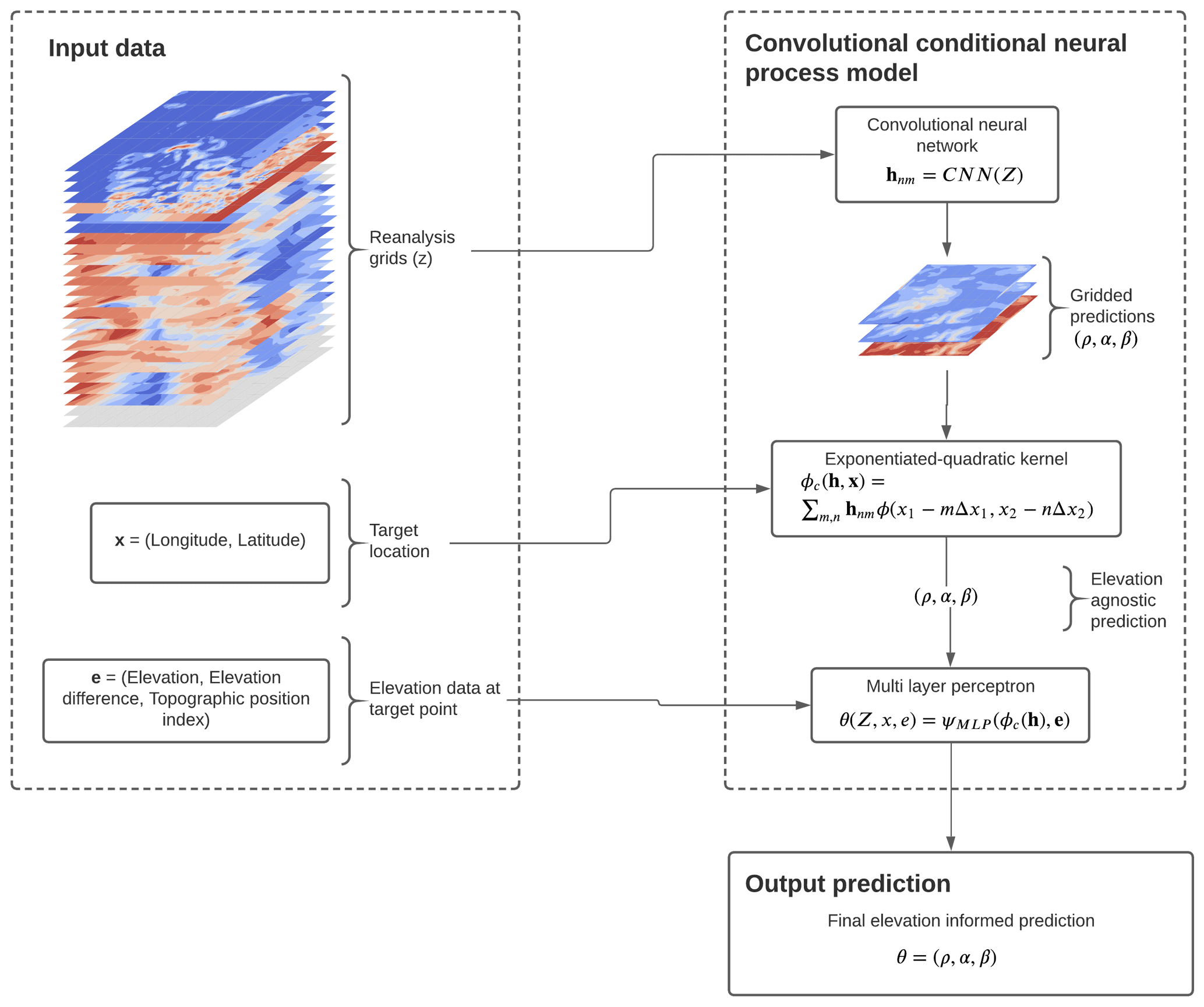
Figure 1Schematic of the convCNP model for downscaling precipitation demonstrating the flow of data in predicting precipitation for a given day at target locations x. Gridded coarse-resolution data for each predictor are fed into the CNN, producing predictions of at each grid point. These gridded predictions are then transformed to a prediction at the target location using an exponentiated-quadratic kernel. Finally, these elevation agnostic predictions are fed into a multi-layer perceptron together with topographic data e to produce a final prediction of the parameters.
2.1 The downscaling model
Our aim is to approximate the function f in Eq. (1) to predict the value of a downscaled climate variable y at locations x given a set of coarse-scale predictors Z. In order to take the local topography into account, we assume that this function also depends on the local topography at each target point, denoted e, i.e.
In this study, f is modelled as a convCNP (Gordon et al., 2019), a member of the conditional neural process family (Garnelo et al., 2018). A neural process model is a deep-learning model that parameterises a mapping from a discrete input set to a posterior stochastic process as a neural network. This is implemented as an encoder that maps the input set to a latent representation, followed by a decoder that takes the latent representation and a target location as input and outputs the predictive distribution at that location (Dubois et al., 2020). In the context of this downscaling problem, the input set is the low-resolution predictors, the mapping of a neural network, and the output a stochastic process over temperature or precipitation that can be queried at an arbitrary spatial location to generate the downscaled predictions. For spatial problems such as downscaling, a desirable inductive bias in a model is that it is translation equivariant, i.e. the model makes identical predictions if the input data are spatially translated. The convCNP model applied here builds this equivariance into the conditional neural process.
Using the convCNP model, we take a probabilistic approach to specifying f where we include a noise model, and thus
Deterministic predictions are made from this by using, for example, the predictive mean
In this model θ is parameterised as
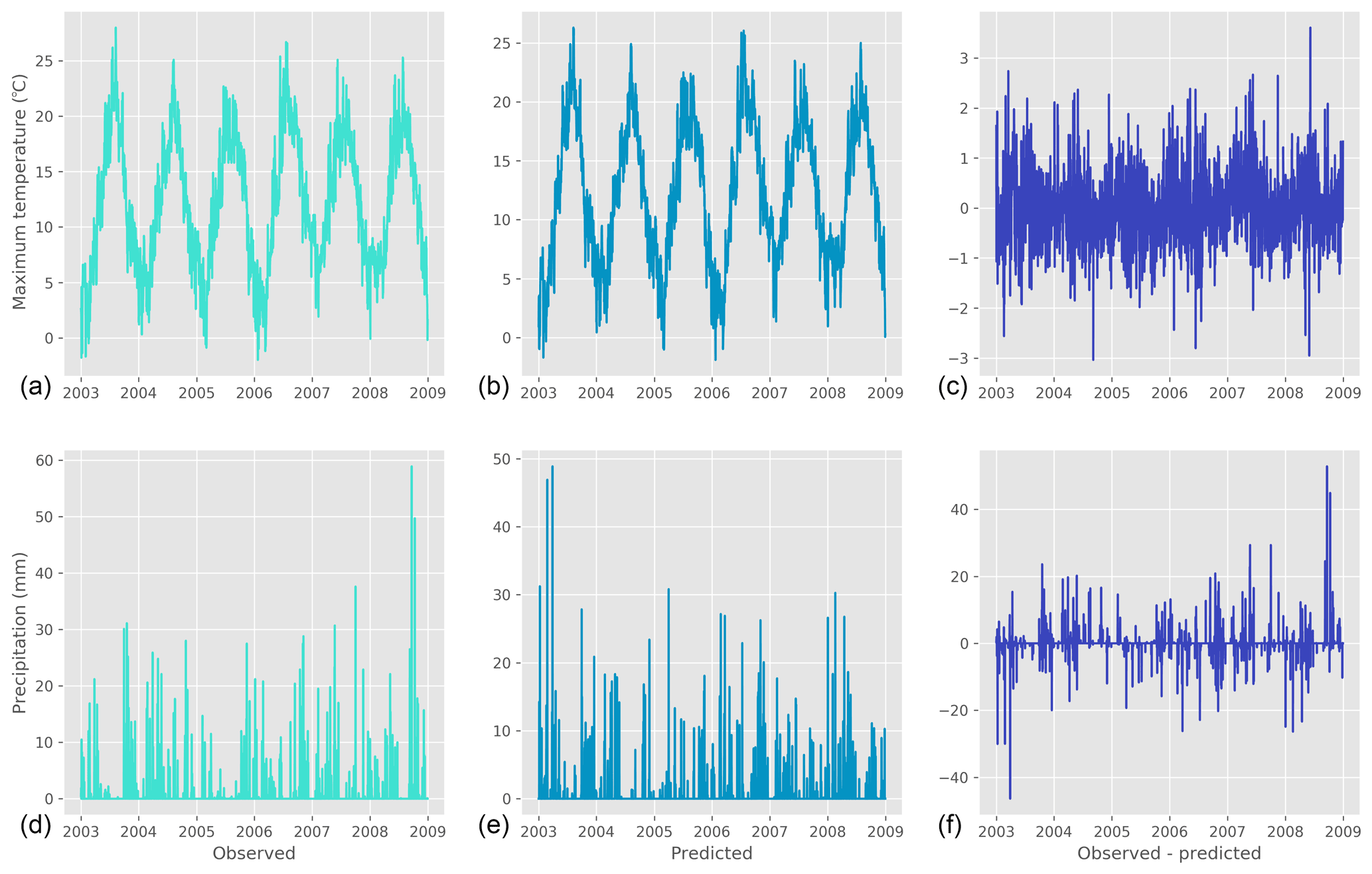
Figure 2Examples of convCNP model predictions compared to observations for (a–c) maximum temperature in Heligoland, Germany, and (d–f) precipitation in Madrid, Spain.
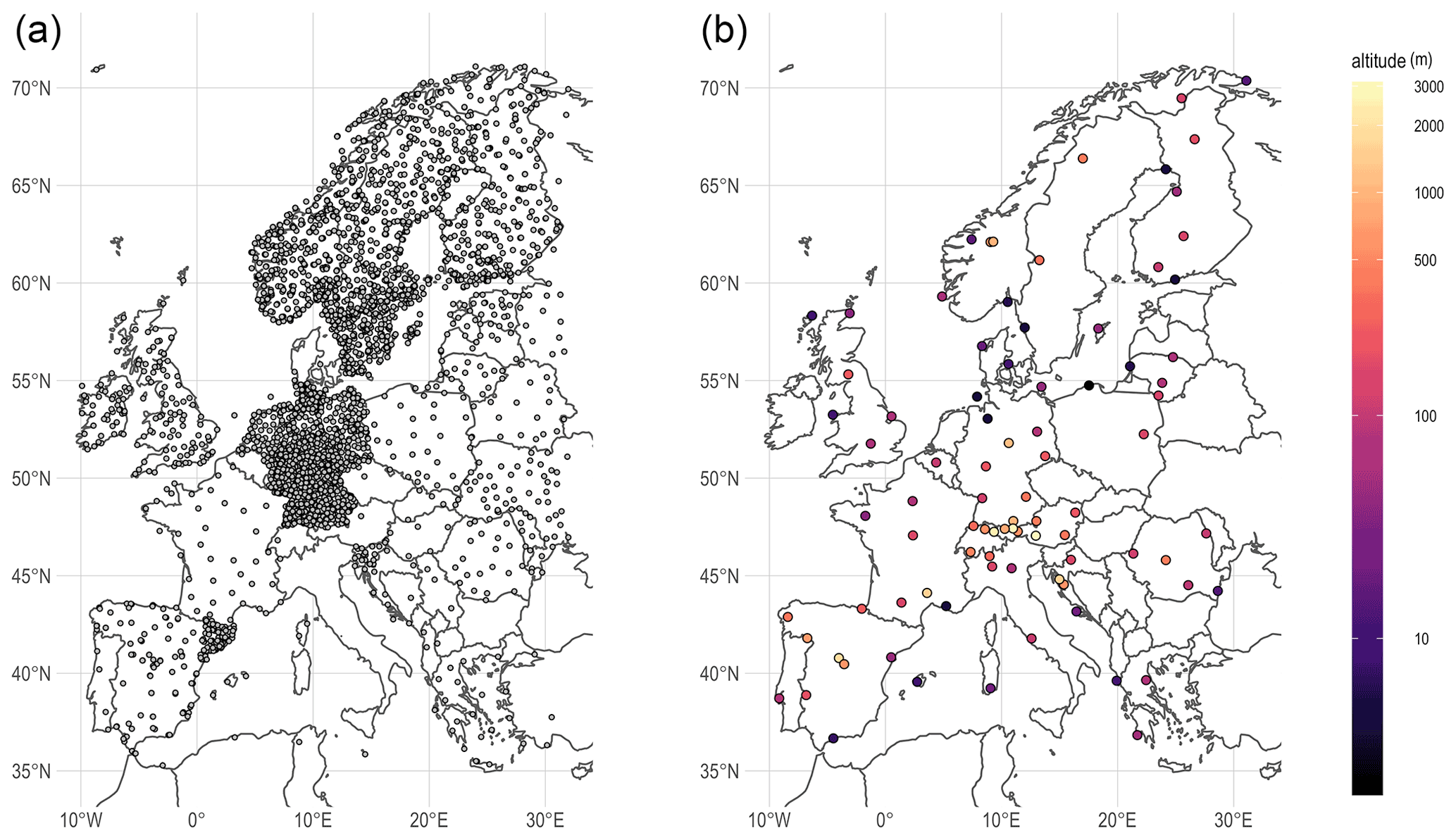
Figure 3Locations of ECA&D (a) and VALUE (b) stations, with altitude shaded.
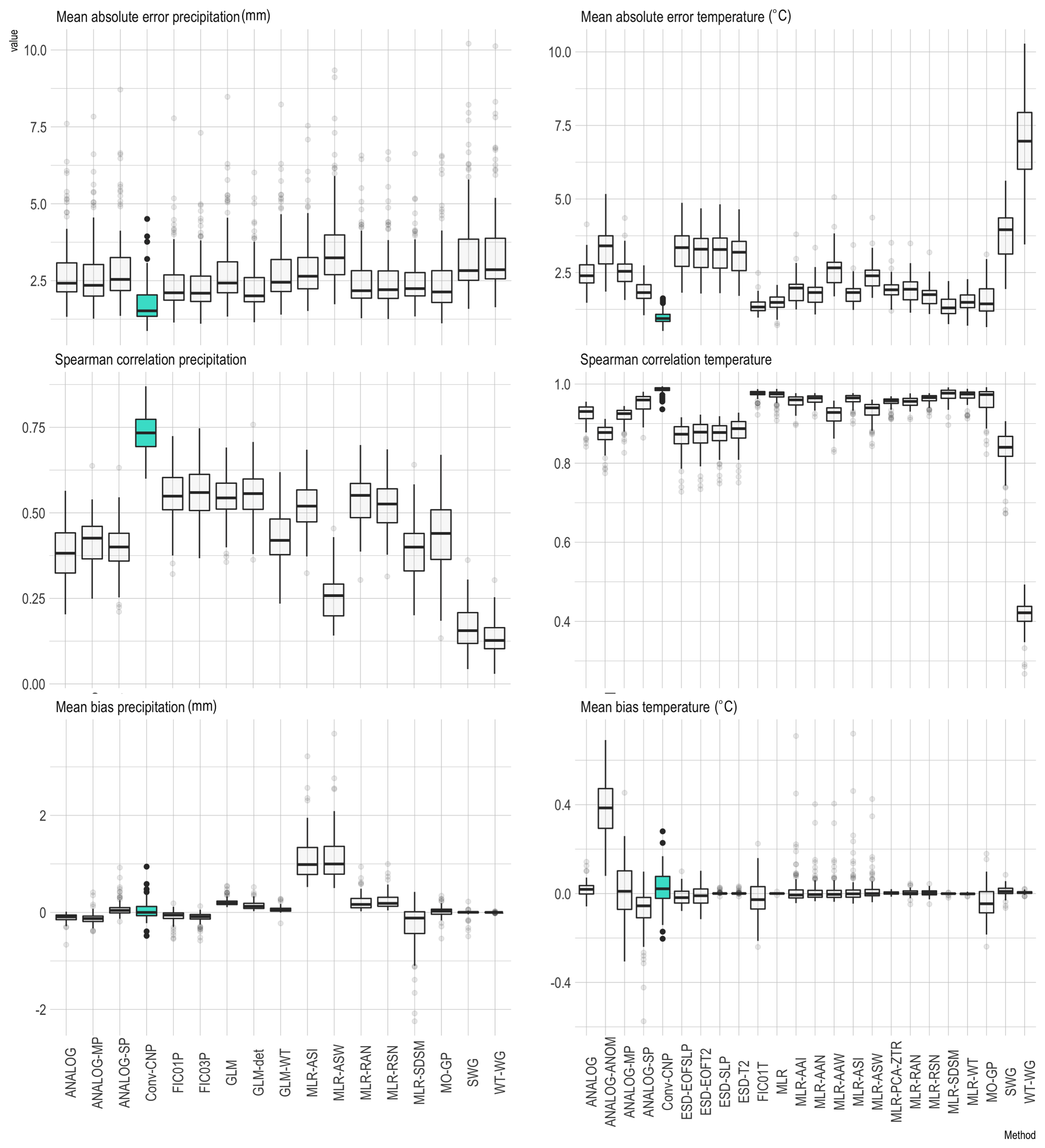
Figure 4Comparison of the convCNP model to VALUE ensemble baselines for mean metrics, with the convCNP model shaded in blue. Each box summarises the performance for one model in the ensemble over the 86 training stations on the held-out validation data.
Here θ is a vector of parameters of a distribution for the climate variable at prediction locations x. Consistent with previous stochastic downscaling studies (Cannon, 2008; Wilks, 2012), this is assumed to be Gaussian for maximum temperature and a Gamma–Bernoulli mixture for precipitation. We note that this is an extension of existing conditional and convolutional conditional neural process models where the predictive distribution is assumed to be Gaussian (Garnelo et al., 2018; Gordon et al., 2019). e is a vector of sub-grid-scale topographic information at each of the prediction locations, ψMLP is a multi-layer perceptron, ϕc is a kernel function with learnable length scale and CNN is a convolutional neural network. Each component of this is described below, with a schematic of the model shown in Fig. 1.
-
Convolutional neural network.
In the first step, daily gridded reanalysis predictor data Z for a single time step are fed into the model. These grids are used as input to a convolutional neural network to extract relevant features. This is implemented as a six-block Resnet architecture (He et al., 2016) with depth-wise separable convolutions (Chollet, 2017). The output from this step is a prediction of the relevant parameters for each variable at each grid point in the predictor set, i.e.where hnm is the vector-valued output at latitude mΔx1 and longitude nΔx2 and with Δxi indicating the grid spacing where the grid consists of M points in the longitude direction and N points in the latitude direction.
-
Translation to off-the-grid predictions.
These gridded predictions are translated to the off-the-grid target locations x using outputs from step 1 as weights for an exponentiated-quadratic (EQ) kernel ϕ, i.e.This outputs predictions of the relevant distributional parameters, θ, at each target location. An EQ kernel is chosen here as it ensures that the predictions are approximately translation equivariant.
-
Inclusion of sub-grid-scale topography
By design, the predictions from the previous step only model variation on the scale of the context grid spacing. This elevation agnostic output is post-processed using a multi-layer perceptron (MLP). This takes the parameter predictions from the EQ kernel as input together with a vector of topographic data e at each target location.The vector e consists of the following three measurements at each target point:
-
true elevation,
-
difference between the true and grid-scale elevation,
-
multi-scale topographic position index (mTPI; measuring the topographic prominence of the location, i.e. quantifying whether the point is in a valley or on a ridge).
This MLP outputs the final prediction of the distributional parameters θ at each target location.
-
Figure 2 shows a concrete example of temperature and precipitation time series produced using this model by sampling from the output distributions. Maximum temperature is shown for Heligoland, Germany, and precipitation is shown for Madrid, Spain. For both variables the model produces qualitatively realistic time series.
2.1.1 Training
The convCNP models are trained by minimising the average negative log likelihood. For temperature, this is given by
where yi is the observed value and denotes a Gaussian distribution over y with mean μi and variance . These parameters are generated by the model at each location xi and use topography ei. N is the total number of target locations. For precipitation, the negative log likelihood is given by
where ri is a Bernoulli random variable describing whether precipitation was observed at the ith target location, yi is the observed precipitation, ρi parameterises the predicted Bernoulli distribution, and is a Gamma distribution with shape parameter αi and scale parameter βi. Here .
Weights are optimised using Adam (Kingma and Ba, 2014), with the learning rate set to 5 × 10⁻⁴. Each model is trained for 100 epochs on 456 batches of 16 d each, using early stopping with a patience of 10 epochs.
2.2 Experiments and datasets
Having addressed the first aim in developing the convCNP model, we next evaluate model performance via three experiments. The first experiment compares the convCNP model to an ensemble of existing downscaling methods following a standardised experimental protocol. In contrast to the convCNP model, these methods are unable to make predictions at locations where training data are not available. In the second experiment, we assess the performance of the convCNP model at these unseen locations compared to a baseline constructed by interpolating single-site models. Finally, ablation experiments are performed to quantify the impact of including sub-grid-scale topographic information on performance.
2.2.1 Experiment 1 – baseline comparison
ConvCNP model performance is first compared to strong baseline methods taken from the VALUE experimental protocol. VALUE (Maraun et al., 2015) provides a standardised suite of experiments to evaluate new downscaling methods, together with data benchmarking the performance of existing methods. In the VALUE 1a experiment, each downscaling method predicts the maximum temperature and daily precipitation at 86 stations across Europe (Fig. 2), given gridded data from the ERA-Interim reanalysis (Dee et al., 2011). These stations are chosen as they offer continuous, high-fidelity data over the training and held-out test periods and represent multiple different climate regimes (Gutiérrez et al., 2019). Data are taken from 1979–2008, with 5-fold cross-validation used over 6-year intervals to produce a 30-year time series.
The convCNPs are trained to predict maximum temperature and precipitation at these 86 VALUE stations given the ERA Interim grids over Europe. Station data are taken from the European Climate Assessment Dataset (Klein Tank et al., 2002). These grids are restricted to points between 35 and 72∘ latitude and −15 to 40∘ longitude. The VALUE experiment protocol does not specify which predictors are used in each downscaling model (i.e. which gridded variables are included in Z), with different predictors chosen for each member of the baseline ensemble, as detailed in Gutiérrez et al. (2019). It is emphasised that in the VALUE baselines a separate model is trained for every location; hence, topographic predictors are not required.
Table 1Gridded predictors from ERA-Interim reanalysis included in Z.
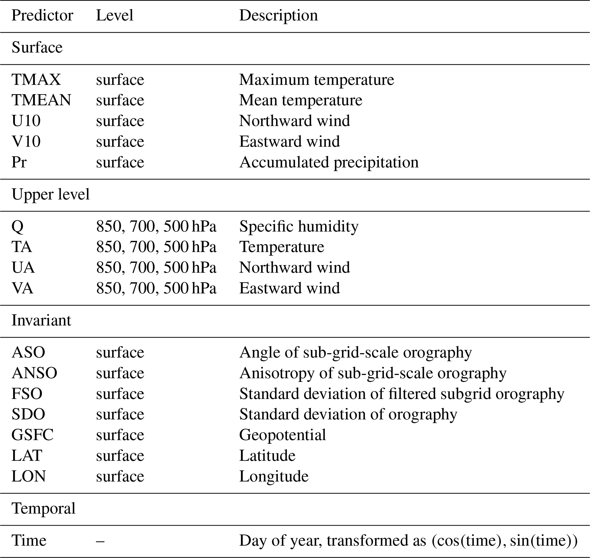
Based on the predictors used by methods in the baseline ensemble, winds, humidity and temperature are included at multiple levels together with time, latitude, longitude and invariant fields. Predictors are summarised in Table 1.
For the sub-grid-scale information for input into the final MLP, the point measurement of three products is provided at each station. True station elevation is taken from the Global Multi-resolution Terrain Elevation Dataset (Danielson and Gesch, 2011). This is provided to the model together with the difference between the ERA-Interim grid-scale resolution elevation and true elevation. Finally, topographic prominence is quantified using the ALOS Global mTPI (Theobald et al., 2015).
Results of the convCNP model are compared to all available PP models in the VALUE ensemble, a total of 16 statistical models for precipitation and 23 for maximum temperature. These models comprise a range of techniques including analogues, multiple linear regression, generalised multiple linear regression and genetic programming. For a complete description of all models included in the comparison, see Appendix A.

Figure 6Comparison of the convCNP model to the GP-baseline. Boxes summarise model performance over the 86 held-out VALUE stations for maximum temperature (a–c) and precipitation (d–f) for each of the mean metrics.
2.2.2 Experiment 2 – performance at unseen locations
We next quantify model performance at unseen locations compared to an interpolation baseline. The convCNP models are retrained using station data from the European Climate Assessment Dataset (ECA&D), comprising 3010 stations for precipitation and 3047 stations for maximum temperature (Fig. 2). The 86 VALUE stations are held out as the validation set, testing the model performance at both unseen times and locations.
As existing downscaling models are unable to handle unseen locations, it is necessary to construct a new baseline. A natural baseline for this problem is to construct individual models for each station using the training set, use these to make predictions at future times and then interpolate to get predictions at the held-out locations. For the single-station models, predictors are taken from ERA-Interim data at the closest grid box, similar to Gutiérrez et al. (2013). Multiple linear regression is used for maximum temperature. For precipitation, occurrence is modelled using logistic regression, and accumulation is modelled using a generalised linear model with gamma error distribution, similar to San-Martín et al. (2017). These methods are chosen as they are amongst the best-performing methods of the VALUE ensemble for each variable (Gutiérrez et al., 2019).
Following techniques used to convert station observations to gridded datasets (Haylock et al., 2008), predictions at these known stations in the future time period are made by first interpolating monthly means (totals) for temperature (precipitation) using a thin-plate spline and then using a GP to interpolate the anomalies (fraction of the total value). All interpolation is three-dimensional over longitude, latitude and elevation. Throughout the results section, this model is referred to as the GP-baseline.
2.2.3 Experiment 3 – topography ablation
Finally, the impact of topography on predictions is quantified. Experiment 2 is repeated three times with different combinations of topographic data fed into the final MLP (step 3 in Fig. 1): no topographic data, elevation and elevation difference only, and mTPI only.

Figure 7Spatial distribution of mean absolute error for convCNP (a, d), GP-baseline (b, e) and convCNP–GP-baseline (c, f). Maximum temperature (precipitation) is shown on the top (bottom) row. All panels show results for each of the 86 held-out VALUE stations.
2.3 Evaluation metrics
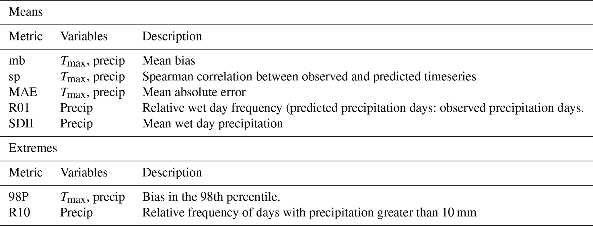
A selection of standard climate metrics are chosen to assess model performance over the evaluation period, quantifying the representation of mean properties and extreme events (Table 2). Metrics are chosen based on those reported for the VALUE baseline ensemble (Gutiérrez et al., 2019; Widmann et al., 2019; Maraun et al., 2019; Hertig et al., 2019).
Comparison to these metrics requires generating a time series of values from the distributions predicted by the convCNP model. For temperature, this is generated by taking the mean of the predicted distribution for mean metrics, and sampling is used to complete the extreme metrics. For precipitation, a day is first classified as wet if ρ≥0.5 or dry if ρ<0.5. For wet days, accumulations are generated by taking the mean of the gamma distribution for mean metrics or sampling for extreme metrics.
The convCNP model outperforms all VALUE baselines on median mean absolute error (MAE) and Spearman correlation for both maximum temperature and precipitation. Comparisons of convCNP model performance at the 86 VALUE stations to each model in the VALUE baseline ensemble are shown in Fig. 4. The low MAE and high Spearman correlation indicate that the model performs well at capturing day-to-day variability.
For maximum temperature, the mean bias is larger than baseline models at many stations, with interquartile range −0.02 to 0.08 ∘C. This is a direct consequence of training a global model as opposed to individual models to each station which will trivially correct the mean (Maraun and Widmann, 2018). Though larger than baseline models, this error is still small for a majority of stations. Similarly for precipitation, though mean biases are larger than many of the VALUE models, the interquartile range is just −0.07 to 0.12 mm. For precipitation, the bias in convCNP relative wet day frequency (R01) and mean wet day precipitation (SDII) are comparable to the best models in the VALUE ensemble (not shown).
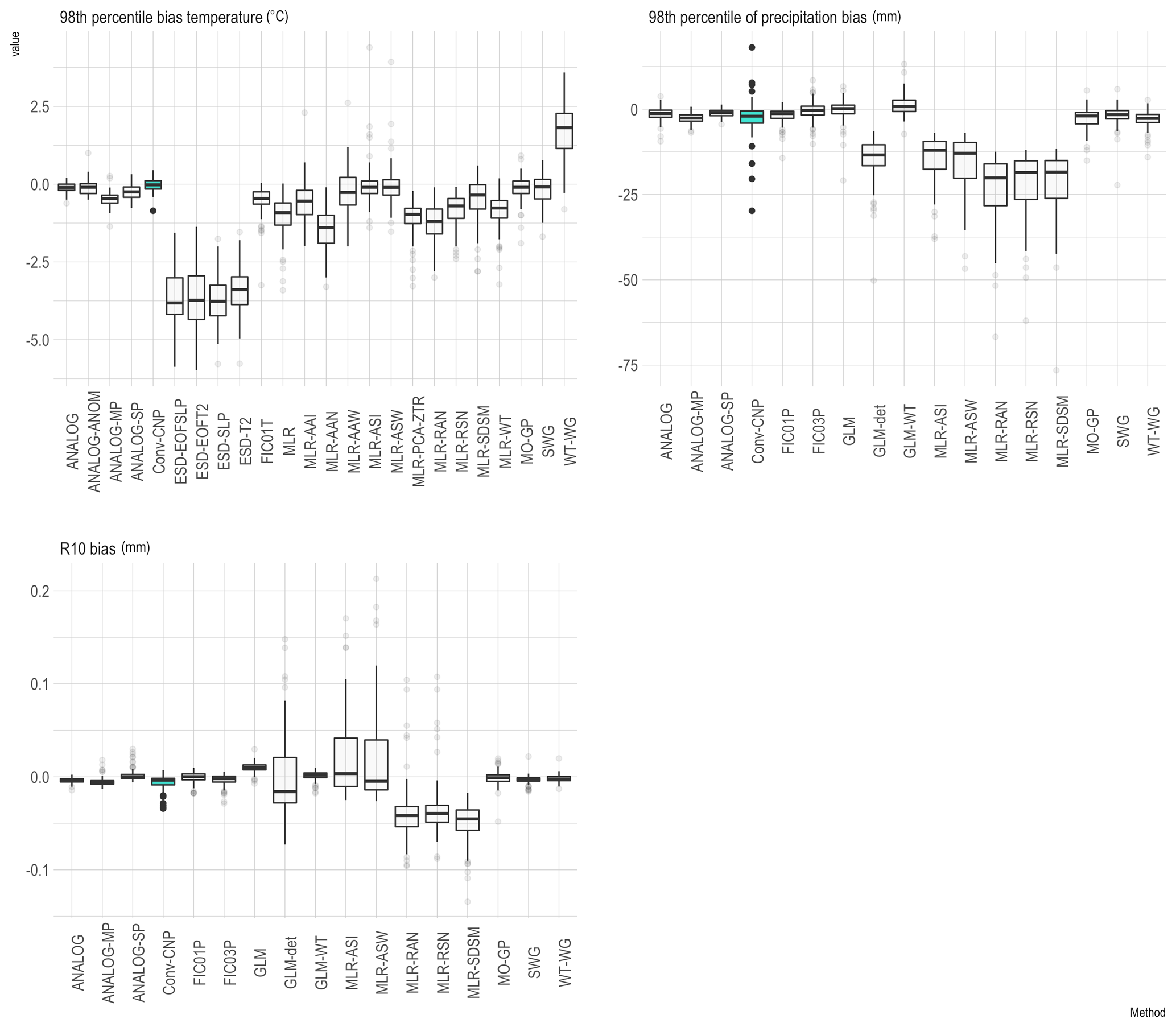
When downscaling GCM output for impact studies, it is of particular importance to accurately reproduce extreme events (Katz and Brown, 1992). In line with previous work comparing the VALUE baselines (Hertig et al., 2019), an extreme event is defined to be a value greater than the 98th percentile of observations. Comparisons of biases in the 98th percentile of maximum temperature and precipitation are shown in Fig. 5. The convCNP performs similarly to the best baselines, with a median bias of −0.02 ∘C for temperature and −2.04 mm for precipitation across the VALUE stations. R10 biases are comparable to baselines, with a median bias of just −0.003 mm.
The convCNP model outperforms the GP-baseline at unseen stations. Results for MAE, Spearman correlation and mean bias are shown in Fig. 6. For maximum temperature, the convCNP model gives small improvements over the baseline model, with Spearman correlations of 0.99 (0.98) and MAE of 1.19 ∘C (1.35 ∘C) for the convCNP (GP baseline). Importantly, large outliers (> 10 ∘C) in the baseline MAE are not observed in the convCNP predictions. Figure 7 shows the spatial distribution of MAE for the convCNP and GP-baseline together with the difference in MAE between the two models. This demonstrates that stations with high MAE in the convCNP model are primarily concentrated in the complex topography of the European Alps. The GP-baseline model displays large MAE not only in the Alps but also at other locations, for example in Spain and France. The convCNP improves predictions at 82 out of the 86 stations.
Repeating this analysis for precipitation, the convCNP model gives substantial improvement over the baseline for MAE and Spearman correlation. Spearman correlations are 0.57 (0.20) and MAE 2.10 mm (2.71 mm) for convCNP (GP-baseline). In contrast to maximum temperature, there is no clear link between topography and MAE, though again convCNP predictions have large MAE for multiple stations located in the Alps. The convCNP model improves on baseline predictions at 80 out of 86 stations.
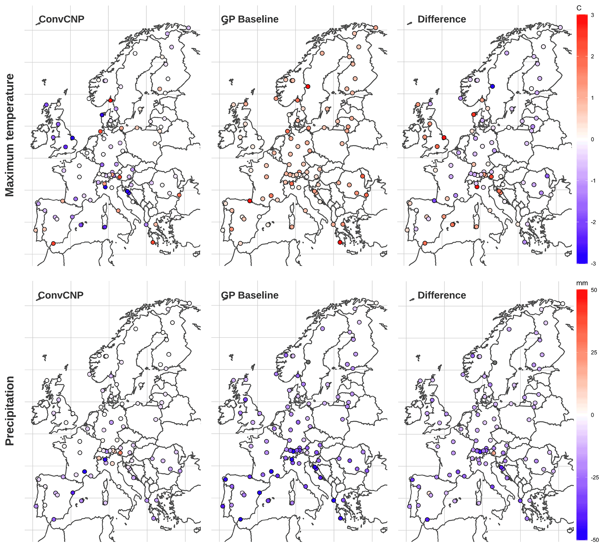
Figure 9The same as for Fig. 7 but for P98 biases. Here, the “difference” panels quantify the difference in absolute bias . Negative (positive) values indicate that the convCNP (GP-baseline) has better performance.
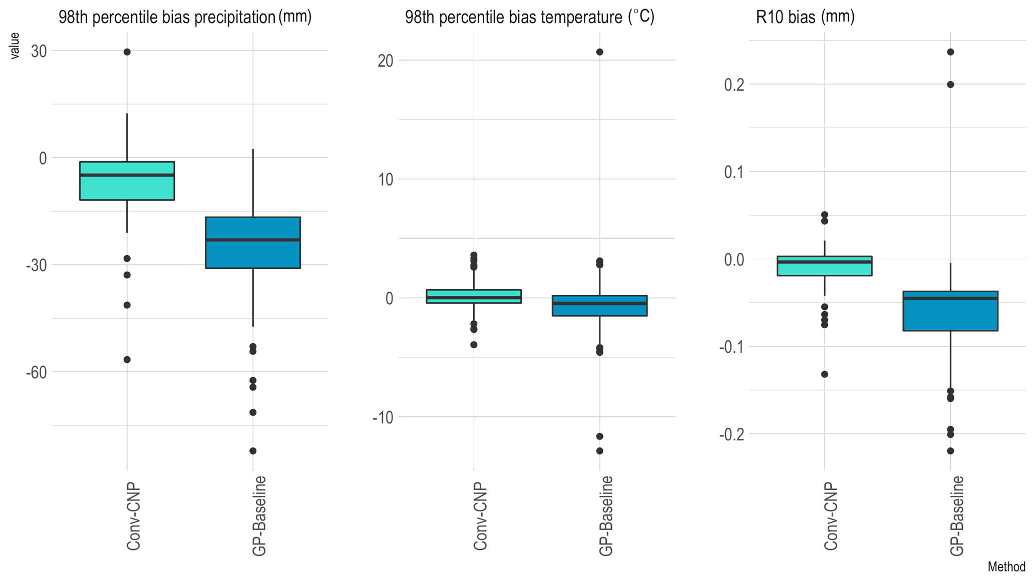
Comparisons between models for extreme metrics are shown in Fig. 8. For maximum temperature, the convCNP has slightly lower absolute 98th percentile bias than the baseline. For precipitation, errors are substantially lower, with median absolute 98th percentile bias of 4.90 mm for convCNP compared to 22.92 mm for GP-baseline. The spatial distributions of 98th percentile bias for maximum temperature and precipitation predictions together with the difference in absolute bias are shown in Fig. 9. For maximum temperature, the convCNP does not improve on the baseline at all stations. The GP-baseline exhibits uniformly positive biases, while the convCNP model has both positive and negative biases. Improvements are seen through central and eastern Europe, while the convCNP performs comparatively poorly in southern Europe and the British Isles. For precipitation, predictions have low biases across much of Europe for the convCNP, with the exception of in the complex terrain of the Alps. GP-baseline biases are negative throughout the domain. For this case, convCNP predictions have lower bias at 84 of the 86 validation stations.
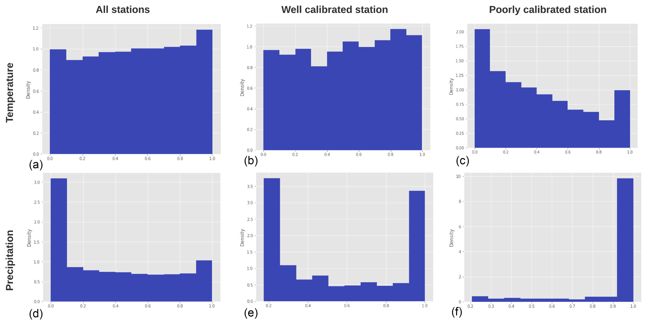
Figure 10Histograms showing probability integral transforms for model predictions compared to a uniform distribution to assess calibration for temperature (a–c) and precipitation (d–f). For temperature PIT plots are shown for all values (a), a station where the model is well calibrated (Bragança, Portugal; b) and a station where the model is poorly calibrated (Gospić, Croatia; c). Similarly for precipitation, PIT plots are shown for all values (d), a station where the model is well calibrated (Stornoway, UK; e) and a station where the model is poorly calibrated (Sodankylä, Finland; f).
A limitation to the analysis of the standard climate metrics in Table 2 is that these only assess certain aspects of the predicted distribution. To assess the calibration of the models, we next examine the probability integral transform (PIT) values. The PIT value for a given prediction is defined as the cumulative density function (CDF) of the distribution predicted by the convCNP model evaluated at the true observed value. These values can be used to determine whether the model is calibrated by evaluating the PIT for every model prediction at the true observation, and plotting their distribution. If the model is properly calibrated, it is both necessary and sufficient for this distribution to be uniform (Gneiting et al., 2007). PIT distributions for maximum temperature and wet-day precipitation are shown in Fig. 10. For temperature, the model is well calibrated overall, although the predicted distributions are often too narrow, as demonstrated by the peaks around zero and one indicating that the observed value falls outside the predicted normal distribution. Calibration of the precipitation model is poorer overall. The peak in PIT mass around zero indicates that this model often over-predicts rainfall accumulation. Performance varies between individual stations for both temperature and precipitation, with examples of PIT distributions for both well-calibrated and poorly calibrated stations shown in Fig. 10.
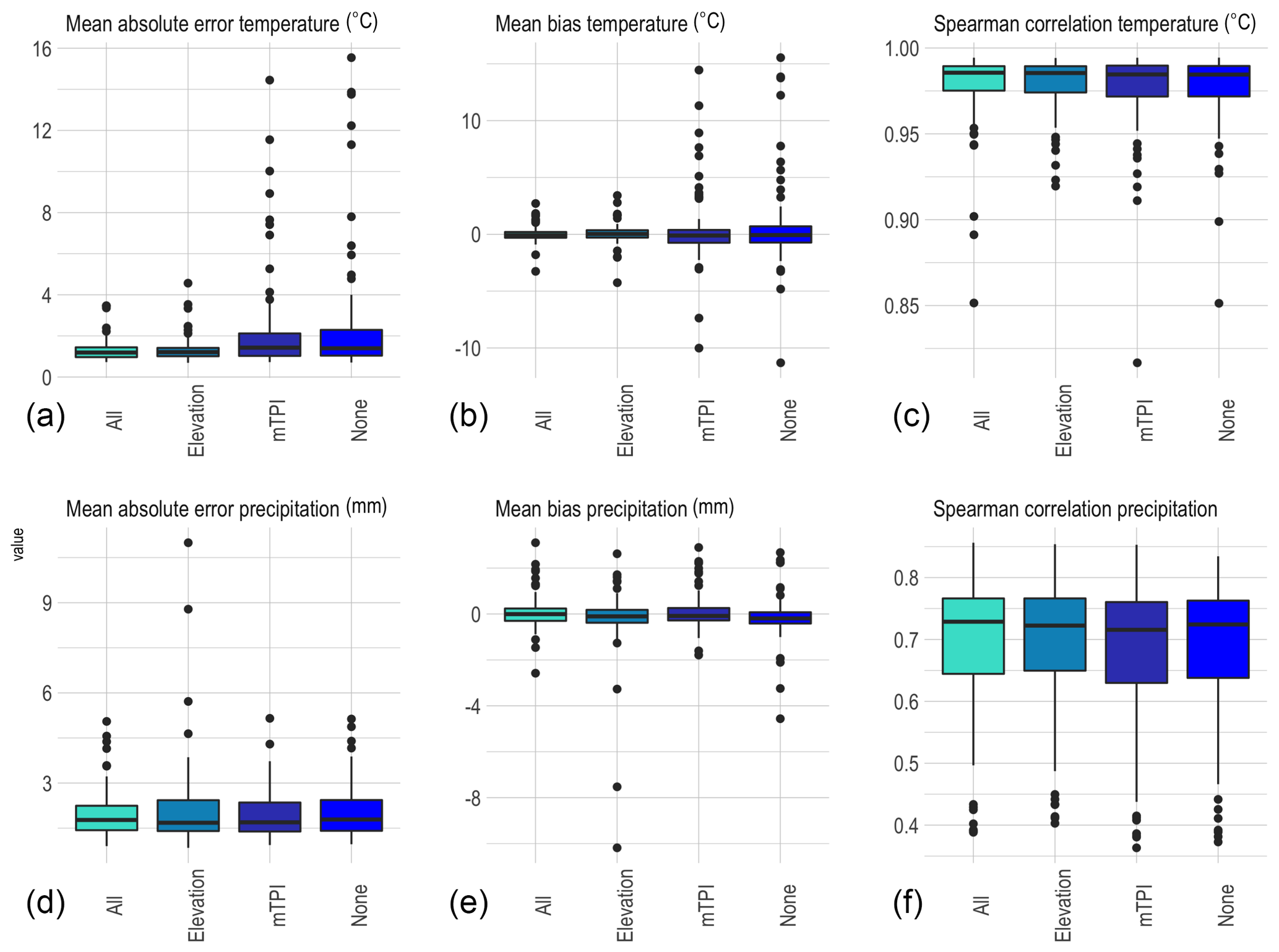
Figure 11Comparison of model performance in the topography ablation experiment. The complete model (All) is compared to models with no topographic data (None), elevation and elevation difference only (Elevation) and mTPI only (mTPI). Boxes summarise model performance over the 86 held-out VALUE stations for maximum temperature (a–c) and precipitation (d–f) for each of the mean metrics.
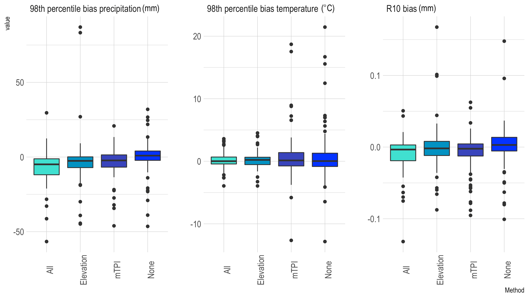
Results of the topography ablation experiment are shown in Fig. 11 (mean metrics) and Fig. 12 (extreme metrics). These figures compare the performance on each metric between the convCNP model with all topographic predictors and convCNP models trained with no topography, elevation and elevation difference only, and mTPI only.
For maximum temperature, inclusion of topographic information improves MAE, mean bias and Spearman correlation. Models including only mTPI or no topographic predictors have a number of stations with very large MAE, exceeding 10 ∘C at several stations. Unsurprisingly, these stations are found to be located in areas of complex topography in the Alps (not shown). Including elevation both decreases the median MAE and corrects errors at these outliers, with further improvement observed with mTPI added. A similar pattern is seen for mean bias. More modest improvements are seen for precipitation, though inclusion of topographic data does result in slightly improved performance.
For maximum temperature, inclusion of topographic data results in reduced 98th percentile bias. This is primarily as a result of including elevation and elevation difference data, with limited benefit derived from the inclusion of mTPI. In contrast, for precipitation, models with topographic correction perform worse than the elevation agnostic model for both 98th percentile and R10 biases. This reduced performance for precipitation may result from overfitting.
This study demonstrated the successful application of convCNPs to statistical downscaling of temperature and precipitation. The convCNP model performs well compared to strong baselines from the VALUE ensemble on both mean and extreme metrics. For both variables the convCNP model outperforms an interpolation-based baseline. Inclusion of sub-grid-scale topographic information is shown to improve model performance for mean and extreme metrics for maximum temperature and mean metrics for precipitation. The convCNP model has a significant advantage over these baselines in that the output prediction is a continuous function, allowing predictions to be made at an arbitrary (longitude, latitude, elevation) location. Although only temperature and precipitation are considered in this study, the model is easily applied to any climate variable with available station observations, for example wind speed.
Several areas remain for future work, both within the convCNP model and in comparison to other downscaling methods. In the convCNP predictions, representation of certain metrics, notably precipitation extremes requires further improvement, particularly in areas with complex topography. The topography ablation experiments demonstrate that the convCNP P98 bias increases in regions with complex topography. Dynamically, this is likely due to local flow effects such as Föhn winds (Gaffin, 2007; Basist et al., 1994), which depend on the incident angle of the background flow. A possible explanation for this is that the MLP is insufficient to model these effects. Further experimentation with adding a second CNN to capture the sub-grid-scale processes and possibly conditioning predictions of this model on local flow is left as a topic for future research. Another avenue for improving model performance would be to change the distribution predicted by the convCNP. Model calibration results presented in Sect. 4 indicate that the temperature downscaling model could be improved using a distribution with heavier tails. Precipitation model calibration requires improvement, with the model frequently under-predicting wet-day accumulations. A possible explanation for this is that the left-hand tail of the gamma distribution decays rapidly. For cases where the mode of the predicted distribution is greater than zero, small observed accumulations are heavily penalised. Previous work has acknowledged that the Bernoulli–gamma distribution used in this study is not realistic for all sites (Vlček and Huth, 2009) and suggested that representation of precipitation extremes can be improved using a Bernoulli–gamma–generalised Pareto distribution (Ben Alaya et al., 2015; Volosciuk et al., 2017). Future work will explore improving the calibration of the downscaling models using mixture distributions and normalising flows (Rezende and Mohamed, 2015) to improve the calibration of the model. A further possibility for extending the convCNP model would be to explicitly incorporate time by building recurrence into the model (Qin et al., 2019; Singh et al., 2019).
Future work will also focus on developing a standardised framework to compare the convCNP model to a variety of deep-learning baselines, building on the work of (Vandal et al., 2019). Although some studies have indicated that in certain cases deep-learning models offer little advantage over widely used statistical methods such as those included in the VALUE ensemble (Baño-Medina et al., 2020; Vandal et al., 2019), others suggest that deep-learning methods offer improved performance (White et al., 2019; Vandal et al., 2017; Höhlein et al., 2020; Liu et al., 2020; Sachindra et al., 2018; Misra et al., 2018). Further work is required both to rigorously compare the convCNP model to other machine learning models for downscaling and to generate a standardised intercomparison of models more broadly. Examination of a larger set of metrics, particularly for precipitation, would also be beneficial.
The final aspect to consider is extending these promising results downscaling reanalysis data to apply to future climate simulations from GCMs. An in depth analysis of the convCNP model performance on seasonal and annual metrics would be beneficial in informing application to impact scenarios. A limitation in all PP downscaling techniques is that applying a transfer function trained on reanalysis data to a GCM makes the assumption that the predictors included in the context set are realistically simulated in the GCM (Maraun and Widmann, 2018). Future work will aim to address this issue through training a convCNP model directly on RCM or GCM hindcasts available through projects such as EURO-CORDEX (Jacob et al., 2014).
Table A1 summarises the baseline methods in the VALUE ensemble. This information is adapted from Gutiérrez et al. (2019).
(Gutiérrez et al., 2013)(Ayar et al., 2016)(Raynaud et al., 2017)(Raynaud et al., 2017)(Benestad et al., 2015)(Benestad et al., 2015)(Benestad et al., 2015)(Ribalaygua et al., 2013)(Ribalaygua et al., 2013)(San-Martín et al., 2017)(San-Martín et al., 2017)(San-Martín et al., 2017)(Gutiérrez et al., 2013)(Huth et al., 2015)(Huth et al., 2015)(Huth et al., 2015)(Huth et al., 2015)(Huth et al., 2015)(Jacobeit et al., 2014)(Huth et al., 2015)(Huth et al., 2015)(Wilby et al., 2002)(Gutiérrez et al., 2013)(Zerenner et al., 2016)(Ayar et al., 2016)(Gutiérrez et al., 2013)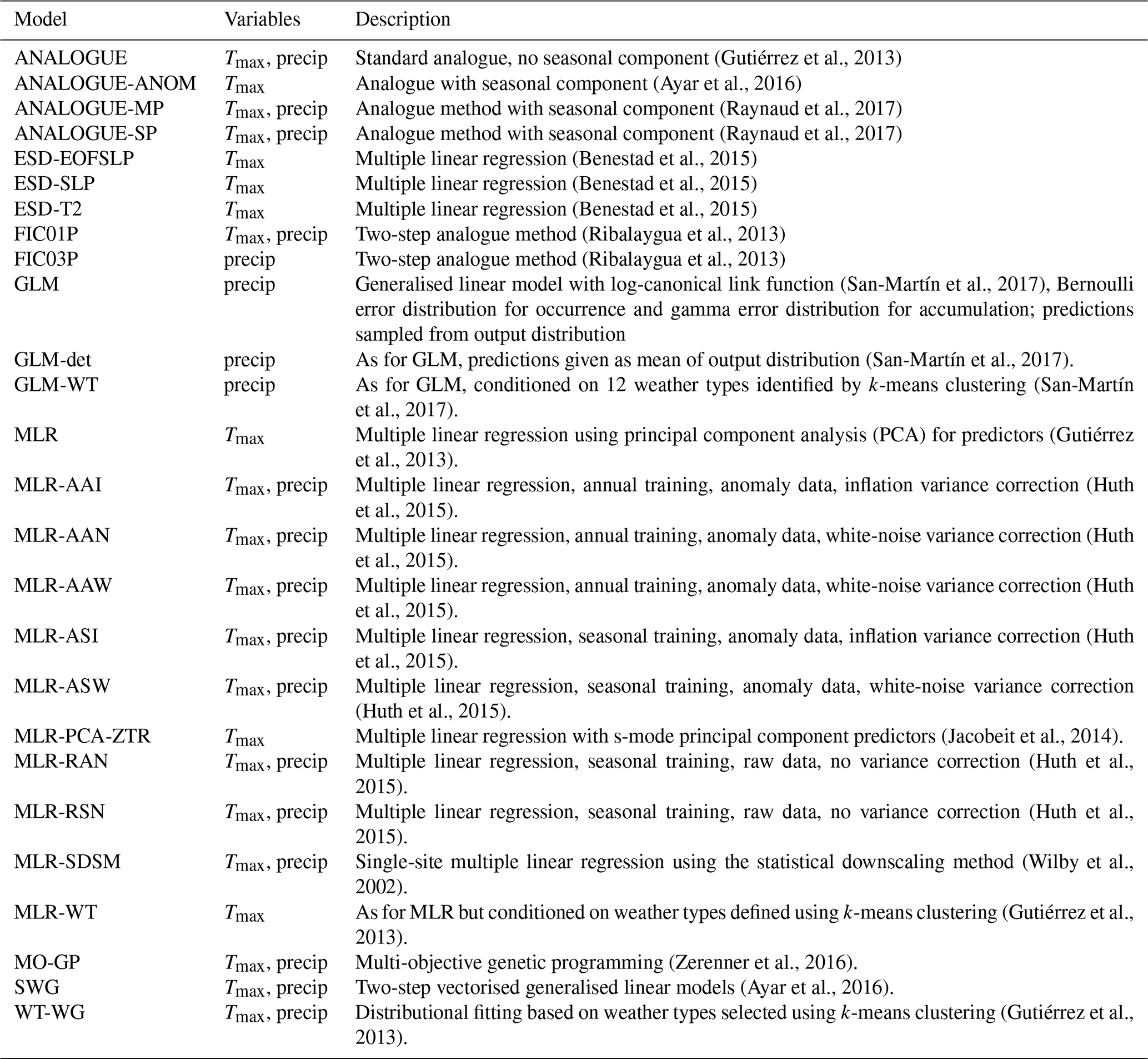
Model code is available at https://github.com/anna-184702/convCNPClimate (last access: 14 December 2020) and https://doi.org/10.5281/zenodo.4554603 (Vaughan, 2021).
ERA-Interim reanalysis data are publicly available at https://apps.ecmwf.int/datasets/data/interim-full-daily/levtype=sfc/ (Dee et al., 2011). Elevation data are available through the Google Earth engine at https://developers.google.com/earth-engine/datasets/catalog/USGS_GMTED2010 (Danielson and Gesch, 2011) and ALOS mTPI https://developers.google.com/earth-engine/datasets/catalog/CSP_ERGo_1_0_Global_ALOS_mTPI (Theobald et al., 2015). ECA&D observations are available at https://www.ecad.eu/dailydata/index.php (Klein Tank et al., 2002).
AV implemented the code, conducted the experiments and wrote the first draft. All authors designed the study and contributed to the analysis of results and final version of the paper.
The authors declare that they have no conflict of interest.
Publisher's note: Copernicus Publications remains neutral with regard to jurisdictional claims in published maps and institutional affiliations.
Anna Vaughan acknowledges the UKRI Centre for Doctoral Training in the Application of Artificial Intelligence to the study of Environmental Risks (AI4ER), led by the University of Cambridge and British Antarctic Survey, and studentship funding from Google DeepMind. Will Tebbutt is supported by Google DeepMind.
This research has been supported by the UKRI Centre for Doctoral Training in the Application of Artificial Intelligence to the study of Environmental Risks (AI4ER), led by the University of Cambridge and British Antarctic Survey, and by Google DeepMind.
This paper was edited by Simone Marras and reviewed by two anonymous referees.
Allen, S., Boschung, J., Nauels, A., Xia, Y., Bex, V., and Midgley, P.: Climate change 2013: the physical science basis. Contribution of working group I to the fifth assessment report of the Intergovernmental Panel on Climate Change, Cambridge University Press, Cambridge, UK, 2016. a
Ayar, P. V., Vrac, M., Bastin, S., Carreau, J., Déqué, M., and Gallardo, C.: Intercomparison of statistical and dynamical downscaling models under the EURO-and MED-CORDEX initiative framework: present climate evaluations, Clim. Dynam., 46, 1301–1329, 2016. a, b, c, d
Baño-Medina, J., Manzanas, R., and Gutiérrez, J. M.: Configuration and intercomparison of deep learning neural models for statistical downscaling, Geosci. Model Dev., 13, 2109–2124, https://doi.org/10.5194/gmd-13-2109-2020, 2020. a, b, c
Basist, A., Bell, G. D., and Meentemeyer, V.: Statistical relationships between topography and precipitation patterns, J. Climate, 7, 1305–1315, 1994. a
Ben Alaya, M. A., Chebana, F., and Ouarda, T. B.: Probabilistic multisite statistical downscaling for daily precipitation using a Bernoulli–generalized pareto multivariate autoregressive model, J. Climate, 28, 2349–2364, 2015. a
Benestad, R. E., Chen, D., Mezghani, A., Fan, L., and Parding, K.: On using principal components to represent stations in empirical–statistical downscaling, Tellus A, 67, 28326, https://doi.org/10.3402/tellusa.v67.28326, 2015. a, b, c
Bevacqua, E., Maraun, D., Hobæk Haff, I., Widmann, M., and Vrac, M.: Multivariate statistical modelling of compound events via pair-copula constructions: analysis of floods in Ravenna (Italy), Hydrol. Earth Syst. Sci., 21, 2701–2723, https://doi.org/10.5194/hess-21-2701-2017, 2017. a
Bhardwaj, A., Misra, V., Mishra, A., Wootten, A., Boyles, R., Bowden, J., and Terando, A. J.: Downscaling future climate change projections over Puerto Rico using a non-hydrostatic atmospheric model, Climatic Change, 147, 133–147, 2018. a, b
Cannon, A. J.: Probabilistic multisite precipitation downscaling by an expanded Bernoulli–Gamma density network, J. Hydrometeorol., 9, 1284–1300, 2008. a, b
Cannon, A. J., Piani, C., and Sippel, S.: Bias correction of climate model output for impact models, chap. 5, in: Climate Extremes and Their Implications for Impact and Risk Assessment, edited by: Sillmann, J., Sippel, S., and Russo, S., Elsevier, 77–104, https://doi.org/10.1016/B978-0-12-814895-2.00005-7, 2020. a
Casanueva, A., Herrera, S., Fernández, J., and Gutiérrez, J. M.: Towards a fair comparison of statistical and dynamical downscaling in the framework of the EURO-CORDEX initiative, Climatic Change, 137, 411–426, 2016. a
Chollet, F.: Xception: Deep learning with depthwise separable convolutions, in: Proceedings of the IEEE conference on computer vision and pattern recognition, 1251–1258, 2017. a
Danielson, J. J. and Gesch, D. B.: Global multi-resolution terrain elevation data 2010 (GMTED2010), U.S. Geological Survey Open-File Report 2011-1073, 26 pp., available at: https://developers.google.com/earth-engine/datasets/catalog/USGS_GMTED2010 (last access: 8 December 2020), 2011. a, b
Dee, D. P., Uppala, S. M., Simmons, A. J., Berrisford, P., Poli, P., Kobayashi, S., Andrae, U., Balmaseda, M. A., Balsamo, G., Bauer, P., Bechtold, P., Beljaars, A. C. M., van de Berg, L., Bidlot, J., Bormann, N., Delsol, C., Dragani, R., Fuentes, M., Geer, A. J., Haimberger, L., Healy, S. B., Hersbach, H., Hólm, E. V., Isaksen, L., Kållberg, P., Köhler, M., Matricardi, M., McNally, A. P., Monge-Sanz, B. M., Morcrette, J.-J., Park, B.-K., Peubey, C., de Rosnay, P., Tavolato, C., Thépaut, J.-N., and Vitart, F.: The ERA-Interim reanalysis: Configuration and performance of the data assimilation system, Q. J. Roy. Meteor. Soc., 137, 553–597, https://doi.org/10.1002/qj.828, 2011 (data available at: https://apps.ecmwf.int/datasets/data/interim-full-daily/levtype=sfc/, last access: 7 December 2020). a, b
Dubois, Y., Gordon, J., and Foong, A. Y.: Neural Process Family, available at: http://yanndubs.github.io/Neural-Process-Family/, last access: 10 December 2020. a
Gaffin, D. M.: Foehn winds that produced large temperature differences near the southern Appalachian Mountains, Weather Forecast., 22, 145–159, 2007. a
Garnelo, M., Rosenbaum, D., Maddison, C. J., Ramalho, T., Saxton, D., Shanahan, M., Teh, Y. W., Rezende, D. J., and Eslami, S.: Conditional neural processes, arXiv [preprint], arXiv:1807.01613, 2018. a, b
Ghosh, S. and Mujumdar, P. P.: Statistical downscaling of GCM simulations to streamflow using relevance vector machine, Adv. Water Resour., 31, 132–146, 2008. a
Gneiting, T., Balabdaoui, F., and Raftery, A. E.: Probabilistic forecasts, calibration and sharpness, J. R. Stat. Soc. B, 69, 243–268, 2007. a
Gordon, J., Bruinsma, W. P., Foong, A. Y., Requeima, J., Dubois, Y., and Turner, R. E.: Convolutional conditional neural processes, arXiv [preprint], arXiv:1910.13556, 2019. a, b, c
Groenke, B., Madaus, L., and Monteleoni, C.: ClimAlign: Unsupervised statistical downscaling of climate variables via normalizing flows, in: Proceedings of the 10th International Conference on Climate Informatics, 60–66, 2020. a
Gutiérrez, J. M., San-Martín, D., Brands, S., Manzanas, R., and Herrera, S.: Reassessing statistical downscaling techniques for their robust application under climate change conditions, J. Climate, 26, 171–188, 2013. a, b, c, d, e, f
Gutiérrez, J. M., Maraun, D., Widmann, M., Huth, R., Hertig, E., Benestad, R., Rössler, O., Wibig, J., Wilcke, R., Kotlarski, S., and San Martin, D.: An intercomparison of a large ensemble of statistical downscaling methods over Europe: Results from the VALUE perfect predictor cross-validation experiment, Int. J. Climatol., 39, 3750–3785, 2019. a, b, c, d, e
Hatfield, J. L. and Prueger, J. H.: Temperature extremes: Effect on plant growth and development, Weather and Climate Extremes, 10, 4–10, 2015. a
Haylock, M., Hofstra, N., Klein Tank, A., Klok, E., Jones, P., and New, M.: A European daily high-resolution gridded data set of surface temperature and precipitation for 1950–2006, J. Geophys. Res.-Atmos., 113, D20119, https://doi.org/10.1029/2008JD010201, 2008. a
He, K., Zhang, X., Ren, S., and Sun, J.: Deep residual learning for image recognition, in: Proceedings of the IEEE conference on computer vision and pattern recognition, 770–778, 2016. a
Hertig, E. and Jacobeit, J.: A novel approach to statistical downscaling considering nonstationarities: application to daily precipitation in the Mediterranean area, J. Geophys. Res.-Atmos., 118, 520–533, 2013. a
Hertig, E., Maraun, D., Bartholy, J., Pongracz, R., Vrac, M., Mares, I., Gutiérrez, J. M., Wibig, J., Casanueva, A., and Soares, P. M.: Comparison of statistical downscaling methods with respect to extreme events over Europe: Validation results from the perfect predictor experiment of the COST Action VALUE, Int. J. Climatol., 39, 3846–3867, 2019. a, b
Höhlein, K., Kern, M., Hewson, T., and Westermann, R.: A Comparative Study of Convolutional Neural Network Models for Wind Field Downscaling, arXiv [preprint], arXiv:2008.12257, 2020. a, b, c
Huth, R., Mikšovskỳ, J., Štěpánek, P., Belda, M., Farda, A., Chládová, Z., and Pišoft, P.: Comparative validation of statistical and dynamical downscaling models on a dense grid in central Europe: temperature, Theor. Appl. Climatol., 120, 533–553, 2015. a, b, c, d, e, f, g
Jacob, D., Petersen, J., Eggert, B., Alias, A., Christensen, O. B., Bouwer, L. M., Braun, A., Colette, A., Déqué, M., Georgievski, G., and Georgopoulou, E.: EURO-CORDEX: new high-resolution climate change projections for European impact research, Reg. Environ. Change, 14, 563–578, 2014. a
Jacobeit, J., Hertig, E., Seubert, S., and Lutz, K.: Statistical downscaling for climate change projections in the Mediterranean region: methods and results, Reg. Environ. Change, 14, 1891–1906, 2014. a
Katz, R. W. and Brown, B. G.: Extreme events in a changing climate: variability is more important than averages, Climatic Change, 21, 289–302, 1992. a
Kingma, D. P. and Ba, J.: Adam: A method for stochastic optimization, arXiv [preprint], arXiv:1412.6980, 2014. a
Klein Tank, A. M. G., Wijngaard, J. B., Können, G. P., Böhm, R., Demarée, G., Gocheva, A., Mileta, M., Pashiardis, S., Hejkrlik, L., Kern‐Hansen, C., and Heino, R.: Daily dataset of 20th-century surface air temperature and precipitation series for the European Climate Assessment, Int. J. Climatol., 22, 1441–1453, https://doi.org/10.1002/joc.773, 2002 (data available at: https://www.ecad.eu/dailydata/index.php, last access: 8 December 2020). a, b
Li, Z., Kovachki, N., Azizzadenesheli, K., Liu, B., Bhattacharya, K., Stuart, A., and Anandkumar, A.: Fourier neural operator for parametric partial differential equations, arXiv [preprint], arXiv:2010.08895, 2020a. a
Li, Z., Kovachki, N., Azizzadenesheli, K., Liu, B., Bhattacharya, K., Stuart, A., and Anandkumar, A.: Neural operator: Graph kernel network for partial differential equations, arXiv [preprint], arXiv:2003.03485, 2020b. a
Liu, Y., Ganguly, A. R., and Dy, J.: Climate Downscaling Using YNet: A Deep Convolutional Network with Skip Connections and Fusion, in: Proceedings of the 26th ACM SIGKDD International Conference on Knowledge Discovery & Data Mining, 3145–3153, 2020. a, b
Lu, L., Jin, P., and Karniadakis, G. E.: Deeponet: Learning nonlinear operators for identifying differential equations based on the universal approximation theorem of operators, arXiv [preprint], arXiv:1910.03193, 2019. a
Maraun, D.: Bias correction, quantile mapping, and downscaling: Revisiting the inflation issue, J. Climate, 26, 2137–2143, 2013. a
Maraun, D. and Widmann, M.: Statistical downscaling and bias correction for climate research, Cambridge University Press, Cambridge, UK, 2018. a, b, c, d, e
Maraun, D., Wetterhall, F., Ireson, A. M., Chandler, R. E., Kendon, E. J., Widmann, M., Brienen, S., Rust, H. W., Sauter, T., Themeßl, M., and Venema, V. K. C.: Precipitation downscaling under climate change: Recent developments to bridge the gap between dynamical models and the end user, Rev. Geophys., 48, RG3003, https://doi.org/10.1029/2009RG000314, 2010. a
Maraun, D., Widmann, M., Gutiérrez, J. M., Kotlarski, S., Chandler, R. E., Hertig, E., Wibig, J., Huth, R., and Wilcke, R. A.: VALUE: A framework to validate downscaling approaches for climate change studies, Earths Future, 3, 1–14, 2015. a
Maraun, D., Shepherd, T. G., Widmann, M., Zappa, G., Walton, D., Gutiérrez, J. M., Hagemann, S., Richter, I., Soares, P. M., Hall, A., and Mearns, L. O.: Towards process-informed bias correction of climate change simulations, Nat. Clim. Change, 7, 764–773, 2017. a, b
Maraun, D., Huth, R., Gutiérrez, J. M., Martín, D. S., Dubrovsky, M., Fischer, A., Hertig, E., Soares, P. M., Bartholy, J., Pongrácz, R., and Widmann, M.: The VALUE perfect predictor experiment: evaluation of temporal variability, Int. J. Climatol., 39, 3786–3818, 2019. a
Mehrotra, R. and Sharma, A.: A nonparametric nonhomogeneous hidden Markov model for downscaling of multisite daily rainfall occurrences, J. Geophys. Res.-Atmos., 110, D16108, https://doi.org/10.1029/2004JD005677, 2005. a
Misra, S., Sarkar, S., and Mitra, P.: Statistical downscaling of precipitation using long short-term memory recurrent neural networks, Theor. Appl. Climatol., 134, 1179–1196, 2018. a, b, c
Pan, B., Hsu, K., AghaKouchak, A., and Sorooshian, S.: Improving precipitation estimation using convolutional neural network, Water Resour. Res., 55, 2301–2321, 2019. a
Piani, C., Haerter, J., and Coppola, E.: Statistical bias correction for daily precipitation in regional climate models over Europe, Theor. Appl. Climatol., 99, 187–192, 2010. a
Qin, S., Zhu, J., Qin, J., Wang, W., and Zhao, D.: Recurrent attentive neural process for sequential data, arXiv [preprint], arXiv:1910.09323, 2019. a
Raynaud, D., Hingray, B., Zin, I., Anquetin, S., Debionne, S., and Vautard, R.: Atmospheric analogues for physically consistent scenarios of surface weather in Europe and Maghreb, Int. J. Climatol., 37, 2160–2176, 2017. a, b
Rezende, D. J. and Mohamed, S.: Variational inference with normalizing flows, arXiv [preprint], arXiv:1505.05770, 2015. a
Ribalaygua, J., Torres, L., Pórtoles, J., Monjo, R., Gaitán, E., and Pino, M.: Description and validation of a two-step analogue/regression downscaling method, Theor. Appl. Climatol., 114, 253–269, 2013. a, b
Sachindra, D., Ahmed, K., Rashid, M. M., Shahid, S., and Perera, B.: Statistical downscaling of precipitation using machine learning techniques, Atmos. Res., 212, 240–258, 2018. a, b
San-Martín, D., Manzanas, R., Brands, S., Herrera, S., and Gutiérrez, J. M.: Reassessing model uncertainty for regional projections of precipitation with an ensemble of statistical downscaling methods, J. Climate, 30, 203–223, 2017. a, b, c, d, e
Singh, G., Yoon, J., Son, Y., and Ahn, S.: Sequential Neural Processes, arXiv [preprint], arXiv:1906.10264, 27 October 2019. a
Teutschbein, C. and Seibert, J.: Bias correction of regional climate model simulations for hydrological climate-change impact studies: Review and evaluation of different methods, J. Hydrol., 456, 12–29, 2012. a
Theobald, D. M., Harrison-Atlas, D., Monahan, W. B., and Albano, C. M.: Ecologically-relevant maps of landforms and physiographic diversity for climate adaptation planning, PLoS One, 10, e0143619, https://doi.org/10.1371/journal.pone.0143619, 2015 (data available at: https://developers.google.com/earth-engine/datasets/catalog/CSP_ERGo_1_0_Global_ALOS_mTPI, last access: 9 December 2020). a, b
Vandal, T., Kodra, E., Ganguly, S., Michaelis, A., Nemani, R., and Ganguly, A. R.: Deepsd: Generating high resolution climate change projections through single image super-resolution, in: Proceedings of the 23rd acm sigkdd international conference on knowledge discovery and data mining, 1663–1672, 2017. a, b, c
Vandal, T., Kodra, E., Dy, J., Ganguly, S., Nemani, R., and Ganguly, A. R.: Quantifying uncertainty in discrete-continuous and skewed data with Bayesian deep learning, in: Proceedings of the 24th ACM SIGKDD International Conference on Knowledge Discovery & Data Mining, 2377–2386, 2018. a
Vandal, T., Kodra, E., and Ganguly, A. R.: Intercomparison of machine learning methods for statistical downscaling: the case of daily and extreme precipitation, Theor. Appl. Climatol., 137, 557–570, 2019. a, b, c
Vaughan, A.: annavaughan/convCNPClimate: First release (v1.0.0), Zenodo [code], https://doi.org/10.5281/zenodo.4554603, 2021. a
Vlček, O. and Huth, R.: Is daily precipitation Gamma-distributed?: Adverse effects of an incorrect use of the Kolmogorov–Smirnov test, Atmos. Res., 93, 759–766, 2009. a
Volosciuk, C., Maraun, D., Vrac, M., and Widmann, M.: A combined statistical bias correction and stochastic downscaling method for precipitation, Hydrol. Earth Syst. Sci., 21, 1693–1719, https://doi.org/10.5194/hess-21-1693-2017, 2017. a
Wang, F., Tian, D., Lowe, L., Kalin, L., and Lehrter, J.: Deep Learning for Daily Precipitation and Temperature Downscaling, Water Resour. Res., 57, e2020WR029308, https://doi.org/10.1029/2020WR029308, 2021. a
White, B., Singh, A., and Albert, A.: Downscaling Numerical Weather Models with GANs, in: AGU Fall Meeting Abstracts, vol. 2019, GC43D–1357, 2019. a, b
Widmann, M., Bedia, J., Gutiérrez, J. M., Bosshard, T., Hertig, E., Maraun, D., Casado, M. J., Ramos, P., Cardoso, R. M., Soares, P. M., and Ribalaygua, J.: Validation of spatial variability in downscaling results from the VALUE perfect predictor experiment, Int. J. Climatol., 39, 3819–3845, 2019. a
Wilby, R. L., Dawson, C. W., and Barrow, E. M.: SDSM?a decision support tool for the assessment of regional climate change impacts, Environ. Modell. Softw., 17, 145–157, 2002. a
Wilks, D. S.: Stochastic weather generators for climate-change downscaling, part II: multivariable and spatially coherent multisite downscaling, WIREs Clim. Change, 3, 267–278, 2012. a
Zerenner, T., Venema, V., Friederichs, P., and Simmer, C.: Downscaling near-surface atmospheric fields with multi-objective Genetic Programming, Environ. Modell. Softw., 84, 85–98, 2016. a
- Abstract
- Introduction
- Datasets and methodology
- Results: baseline comparison (experiment 1)
- Results: performance at unseen locations (experiment 2)
- Results: topography ablation (experiment 3)
- Discussion and conclusion
- Appendix A: VALUE ensemble methods
- Code availability
- Data availability
- Author contributions
- Competing interests
- Disclaimer
- Acknowledgements
- Financial support
- Review statement
- References