The effects of ocean surface waves on global intraseasonal prediction: case studies with a coupled CFSv2.0–WW3 system

This article describes the implementation of a coupling between a global forecast model (CFSv2.0) and a wave model (WW3) and investigates the effects of ocean surface waves on the air–sea interface in the new framework. Several major wave-related processes, including the Langmuir mixing, the Stokes–Coriolis force with entrainment, air–sea fluxes modified by the Stokes drift, and momentum roughness length, are evaluated in two groups of 56 d experiments, one for boreal winter and the other for boreal summer. Comparisons are made against in situ buoys, satellite measurements, and reanalysis data to evaluate the influence of waves on intraseasonal prediction of sea surface temperature (SST), 2 m air temperature (T02), mixed layer depth (MLD), 10 m wind speed (WSP10), and significant wave height (SWH). The wave-coupled experiments show that overestimated SSTs and T02s, as well as underestimated MLDs at mid-to-high latitudes in summer from original CFSv2.0, are significantly improved due to enhanced vertical mixing generated by the Stokes drift. For WSP10s and SWHs, the wave-related processes generally reduce biases in regions where WSP10s and SWHs are overestimated. On the one hand, the decreased SSTs stabilize the marine atmospheric boundary layer and weaken WSP10s and then SWHs. On the other hand, the increased roughness length due to waves reduces the originally overestimated WSP10s and SWHs. In addition, the effects of the Stokes drift and current on air–sea fluxes also rectify WSP10s and SWHs. These cases are helpful for the future development of the two-way CFSv2.0–wave coupled system.

1 Introduction

Ocean surface gravity waves play an important role in modifying physical processes at the atmosphere–ocean interface, which can influence momentum, heat, and freshwater fluxes across the air–sea interface (Li and Garrett, 1997; Taylor and Yelland, 2001; Moon et al., 2004; Janssen, 2004; Belcher et al., 2012; Moum and Smyth, 2019). For instance, ocean surface waves modify ocean surface roughness to influence the marine atmospheric boundary layer and thus change the momentum, latent heat, and sensible heat transfer (Janssen, 1989, 1991; Taylor and Yelland, 2001; Moon et al., 2004; Drennan et al., 2003, 2005). The breaking waves inject turbulent kinetic energy into the upper ocean, which enhances the mixing process (Terray et al., 1996). Nonbreaking surface waves also affect mixing in the upper ocean by adding a wave-related Reynolds stress (Qiao et al., 2004; Ghantous and Babanin, 2014). The wave-related Stokes drift interacts with the Coriolis force and produces the Stokes–Coriolis force (Hasselmann, 1970). The shear of the Stokes drift is critical for generation of Langmuir circulation, which significantly deepens the mixed layer by strong vertical mixing both at climate scales (Li and Garrett, 1997; Belcher et al., 2012) and at weather scales (Kukulka et al., 2009).

Various wave-related parameterizations have been proposed and used in modeling. The wave-related Charnock parameter (C_ch) defines sea surface roughness and affects wind stress estimates (Pineau-Guillou et al., 2018; Sauvage et al., 2020). There are primarily three methods for defining C_ch, considering the wave-induced kinematic stress (Janssen, 1989, 1991), the wave age (Drennan et al., 2003, 2005; Moon et al., 2004), or the steepness (Taylor and Yelland, 2001). The first two are based on the wind-sea conditions, whereas the latter includes both swells and wind-sea waves. Modifications to these Charnock parameterizations were suggested in recent studies for leveling off roughness under high winds (e.g., Fan et al., 2012; Bidlot et al., 2020; ECMWF, 2020; Li et al., 2021). In the oceanic boundary layer, waves influence upper ocean mixing via wave dissipation and the Stokes drift-induced processes. In Breivik et al. (2015), the wave dissipation-related turbulent kinetic energy flux is found to yield the largest sea surface temperature (SST) differences in the extratropics. The Stokes drift-induced Langmuir turbulence can improve temperature simulation over most of the world oceans, particularly in the Southern Ocean (Belcher et al., 2012; Li et al., 2016). Polonichko (1997), Van Roekel et al. (2012), and Li et al. (2017) indicated that the Langmuir cell intensity strongly depends on the alignment of winds and waves, reaching a maximum when they are aligned. Li et al. (2016) found that the effect of Langmuir cell can be further enhanced by entrainment. In Couvelard et al. (2020), the Stokes drift-related forces can also contribute modestly to deepening of the mixed layer depth (MLD). In the First Institute of Oceanography Earth System Model, Bao et al. (2019) indicated that the nonbreaking wave-induced mixing, the Stokes drift-affected air–sea fluxes, and sea spray are all important for climate estimates.

The wave-related processes at the air–sea interface are complex and important in global coupled systems (e.g., Breivik et al., 2015; Law-Chune and Aouf, 2018; Bao et al., 2019; Couvelard et al., 2020). Most of the coupled models with a wave component at global scale were developed for climate research (e.g., Law-Chune and Aouf, 2018; Bao et al., 2019; Couvelard et al., 2020). Exceptionally, an Integrated Forecasting System (IFS) with fully coupled atmosphere, ocean, and wave components, developed by European Centre for Medium-Range Weather Forecasts (ECMWF) (Janssen, 2004; Bidlot, 2019; Bidlot et al., 2020), has been assembled for global forecasts from medium-range weather scales to seasonal scales (Breivik et al., 2015). The National Centers for Environmental Prediction (NCEP) is establishing its atmosphere–ocean–wave system, in which the Global Forecast System (GFS; the atmosphere module in the Climate Forecast System model version 2.0) is one-way coupled with WAVEWATCH III (WW3).

The effects of wave-related processes are worth further evaluation in different global coupled modeling systems. Since it takes significant time for the wave energy to develop (Janssen, 2004), we investigate the impact of individual wave processes at intraseasonal timescale in a new global atmosphere–ocean–wave system. To achieve this, we couple WW3 to the Climate Forecast System model version 2.0 (CFSv2.0) and then conduct sensitivity experiments in boreal winter and summer for comparison. The effects of upper ocean mixing modified by Langmuir cell, the Stokes–Coriolis force and entrainment, air–sea fluxes modified by surface current and the Stokes drift, and momentum roughness length are evaluated. The CFSv2.0 is a coupled system mainly applied for intraseasonal and seasonal prediction (e.g., Saha et al., 2014). Our work can provide insights into two-way wave coupling of CFSv2.0 and is helpful for the future development of the CFSv2.0–wave coupling system. Two groups of 56 d predictions are conducted for boreal winter and boreal summer. Then, the predictions are compared with observations and reanalysis data. For each group, sensitivity experiments with different wave parameterizations are carried out to evaluate the effects of individual wave-related process.

The rest of the paper is structured as follows: methods and numerical experiments with different parameterizations are described in Sect. 2; the observations and reanalysis data are introduced in Sect. 3, and the results of experiments are evaluated and compared in Sect. 4. Finally, a summary and discussion are given in Sect. 5.

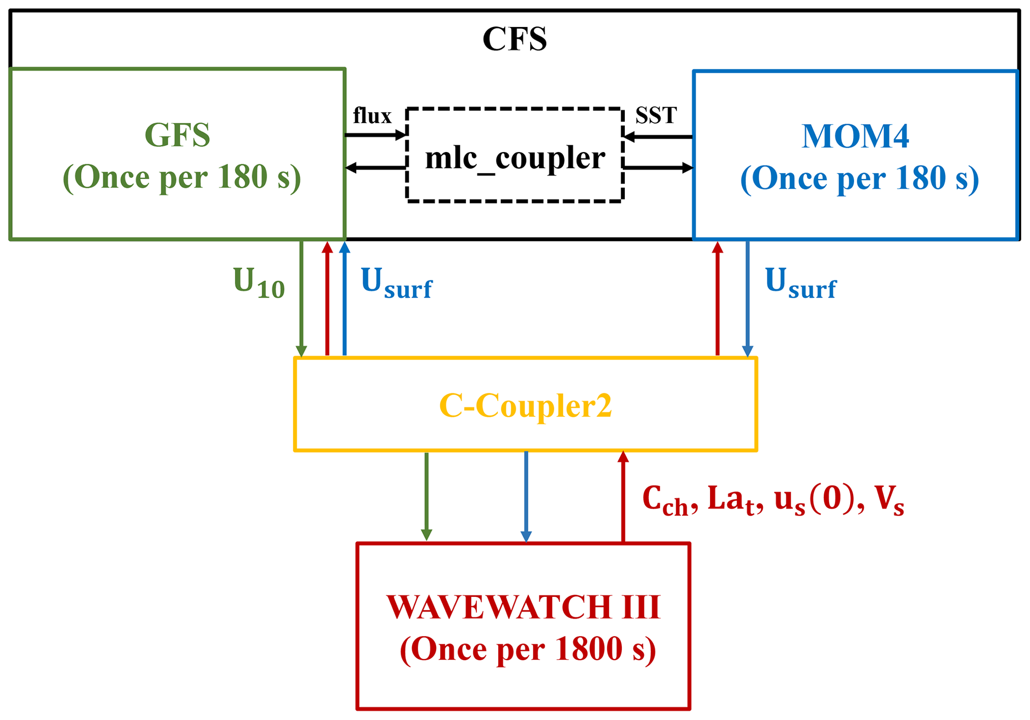
Figure 1 A schematic diagram of the atmosphere–ocean–wave coupled modeling system. The arrows indicate the coupled variables that are passed between the model components. In the diagram, C_ch, La_t, u_s(0), V_s, U₁₀, and U_surf are Charnock parameter (red arrows), turbulent Langmuir number (red arrows), surface Stokes drift velocity (red arrows), Stokes transport (red arrows), 10 m wind (green arrows), and surface current (blue arrows), respectively.

2 Methods and experiments

2.1 Coupling WAVEWATCH III with CFSv2.0

Version 5.16 of WW3 (WAVEWATCH III Development Group, 2016) developed by the National Oceanic and Atmospheric Administration (NOAA)/NCEP has been incorporated into the CFSv2.0 (Saha et al., 2014) as a new model component. The latitude range of WW3 is 78^∘ S–78^∘ N with a spatial resolution of $\mathrm{1}/\mathrm{3}$^∘; the frequency range is 0.04118–0.4056 Hz, and the total number of frequencies is 25; the number of wave directions is 24 with a resolution of 15^∘; the maximum global time step and the minimum source term time step are both 180 s.

The CFSv2.0 contains two components: the GFS (details are available at https://www.emc.ncep.noaa.gov/emc/pages/numerical_forecast_systems/gfs.php, last access: 20 January 2022) as the atmosphere component and the Modular Ocean Model version 4 (MOM4; Griffies et al., 2004) as the ocean component. MOM4 is integrated on a nominal 0.5^∘ horizontal grid with horizontal resolution enhanced to 0.25^∘ in the tropics and has 40 vertical levels; the vertical spacing is 10 m in the upper 225 m, and it then increases in unequal intervals to the bottom at 4478.5 m. A three-layer sea ice model is included in MOM4 (Wu et al., 2005). GFS uses a spectral triangular truncation of 382 waves (T382) in the horizontal, which is equivalent to a grid resolution of nearly 35 km, and 64 sigma–pressure hybrid layers in the vertical. The time steps of both MOM4 and GFS are 180 s. The ocean and atmosphere components are then coupled at the same rate. In the original two-way coupled system, GFS receives SST from MOM4 and sends fluxes of heat, momentum, and freshwater to MOM4 (black arrows in Fig. 1).

The Chinese Community Coupler version 2.0 (C-Coupler2; Liu et al., 2018) is used to interpolate and pass variables between atmosphere and wave components as well as ocean and wave components. Each component receives inputs and supplies outputs on its own grids. The C-Coupler2 is a common, flexible, and user-friendly coupler, which contains a dynamic 3-D coupling system and enables variables to remain conserved after interpolation.

A schematic diagram of the coupled atmosphere–ocean–wave system is shown in Fig. 1. As illustrated, WW3 is two-way coupled with MOM4 and GFS, through the C-Coupler2. WW3 is forced by 10 m wind from GFS (green arrows) and surface current from MOM4 (blue arrows) and generates the wave action density spectrum. Meanwhile, the surface Stokes drift velocity, the Stokes transport, and the turbulent Langmuir number are passed to MOM4 (red arrows; see Sect. 2.3) from WW3, and the surface Stokes drift velocity and the Charnock parameter are passed to GFS (red arrows; see Sect. 2.4 and 2.5). The high-frequency tail assumption for the Stokes drift in WW3 is used with a spectral level decaying as f⁻⁵ (frequency). Additionally, the regular ocean surface current velocities from MOM4 are also passed to GFS to calculate the relative wind velocity for the turbulent fluxes together with the surface Stokes drift (blue arrows; see Sect. 2.4).

Both CFSv2.0 and WW3 use warm starts; the initial fields at 00:00 UTC of the first day in each experiment for CFSv2.0 were generated by the real-time operational Climate Data Assimilation System (Kalnay et al., 1996), downloaded from the CFSv2.0 official website (http://nomads.ncep.noaa.gov/pub/data/nccf/com/cfs/prod, last access: 20 January 2022). To get initial conditions for WW3, a stand-alone WW3 model is set up synchronously (see Sect. 2.2). Since the interactions between waves and sea ice are complicated and beyond the scope of the study, we turn off the coupling between WW3 and CFSv2.0 in areas with sea ice.

In addition, to properly select the coupling frequency between CFSv2.0 and WW3, the root-mean-square errors (RMSEs) of SST, significant wave height (SWH), and 10 m wind speed (WSP10) with different coupling steps for the fully coupled experiment (ALL; details in Sect. 2.6) are calculated and compared (Table S1 of the Supplement). The three components are coupled every time step (180 s) in the 1_STEP_ALL experiment, every 5 steps (900 s) in the 5_STEP_ALL experiment, and every 10 steps (1800 s) in the 10_STEP_ALL experiment. In 10_STEP_WW3, only WW3 is coupled every 10 time steps, whereas GFS and MOM4 remain at the one-time-step (180 s) coupling frequency as in the original settings in CFSv2.0. From Table S1, the 10_STEP_WW3 experiment has a relatively short runtime and small RMSEs. Therefore, the time steps of 10_STEP_WW3 are selected to compromise between computing time and model RMSEs.

2.2 Initialization of WAVEWATCH III

In WW3, input of momentum and energy by wind and dissipation for wave–ocean interaction are two important terms (combined as input–dissipation source term) in the energy balance equation (WAVEWATCH III Development Group, 2016), which includes the estimation of the Charnock parameter. Several different packages to calculate the input–dissipation source term (ST) are available in the WW3 version 5.16, including ST2 (Tolman and Chalikov, 1996), ST3 (Janssen, 2004; Bidlot, 2012), ST4 (Ardhuin et al., 2010), and ST6 (Zieger et al., 2015).

The initial wave fields are generated from 10 d simulation starting from rest in a stand-alone WW3 model. To minimize the biases of initial wave fields, we test simulations with ST2, ST3, ST4, and ST6 schemes and compare the results with Janson-3 observations. Two 10 m wind datasets, the Cross-Calibrated Multi-Platform (CCMP; Atlas et al., 2011) data and the fifth-generation European Centre for Medium-Range Weather Forecasts (ECMWF) Reanalysis (ERA5; Hersbach et al., 2020) data, are used to drive the wave model. Comparing all results, the ST4 scheme with ERA5 wind forcing generates the minimum SWH bias (Table S2 in the Supplement), consistent with findings in Stopa et al. (2016). Thus, the ST4 scheme is chosen to calculate the input and dissipation term and to generate initial wave fields with ERA5 wind forcing for experiments listed in Table 1. The parameters used for the ST4 scheme follow TEST471f from WAVEWATCH III Development Group (2016), which is the CFSR (CFS Reanalysis) tuned setup and is commonly used at the global scale.

Table 1 List of numerical experiments: setups different from control (CTRL) are marked with bold.

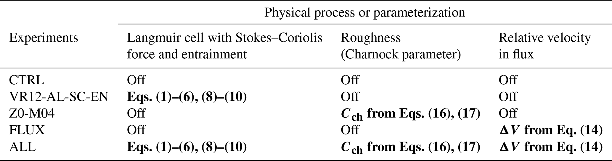
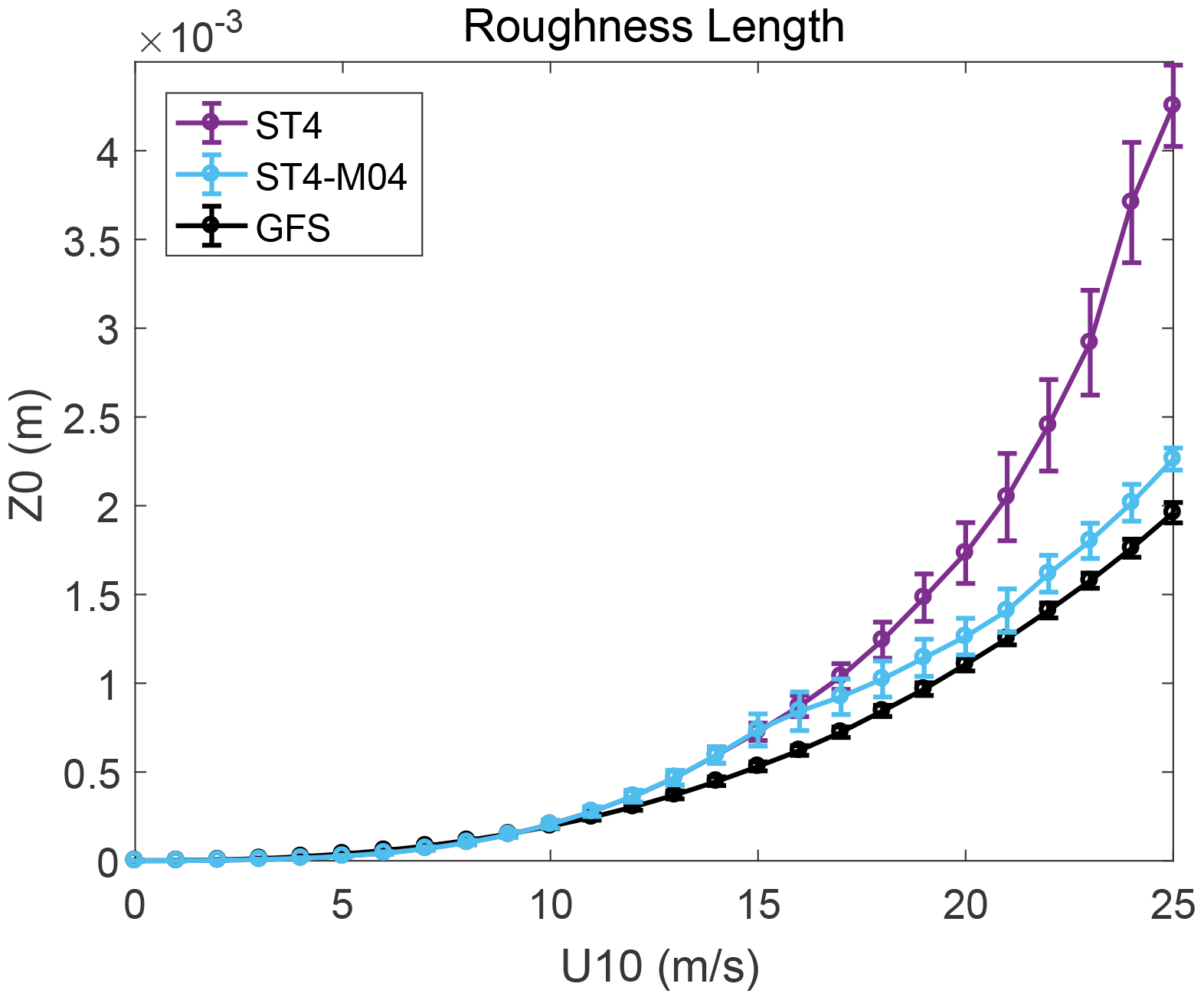
Figure 2 Relationships between momentum roughness length z₀ (m) in the coupled system and 10 m wind speed (m s⁻¹); error bars indicate twice the standard deviations for each point.

2.3 Parameterizations of the Stokes drift-related ocean mixing

The full Stokes drift profile used in MOM4 is obtained by the method by Couvelard et al. (2020), which is based on the work by Breivik et al. (2014, 2016). Breivik et al. (2016) derived the full Stokes drift profile as

$$\begin{array}{}\text{(1)}& u_{\mathrm{s}}\mathrm{B}\mathrm{16}\left(z\right)=u_{\mathrm{s}}\left(\mathrm{0}\right)[\exp \left(\mathrm{2}{k}_{p}z\right)-\sqrt{-\mathrm{2}\mathit{\pi }{k}_{p}z}\mathrm{erfc}(\sqrt{-\mathrm{2}{k}_{p}z}\left)\right],\end{array}$$

where u_s(0) is the surface Stokes drift velocity, $k_p=\frac{u_{\mathrm{s}}\left(\mathrm{0}\right)}{\mathrm{6}{V}_{\mathrm{s}}}$, V_s is the Stokes transport, and erfc is the complementary error function. Equation (1) is depth-averaged within each vertical grid interval as

$$\begin{array}{}\text{(2)}& {\displaystyle }{u}_{\mathrm{s}}\left(z\right)={\displaystyle \frac{u_{\mathrm{s}}\left(\mathrm{0}\right)}{{\left(\mathrm{th}\right)}_k}}[I\left(z_{k+\mathrm{1}/\mathrm{2}},k_p\right)-I\left(z_{k-\mathrm{1}/\mathrm{2}},k_p\right)],\text{(3)}& {\displaystyle }I\left(z,k_p\right)={\displaystyle \frac{\mathrm{1}}{\mathrm{6}{k}_p}}[e^{\mathrm{2}{k}_{p}z}+\mathrm{4}{k}_{p}z{\displaystyle \frac{u_{\mathrm{s}}\mathrm{B}\mathrm{16}\left(z\right)}{u_{\mathrm{s}}\left(\mathrm{0}\right)}}],\end{array}$$

where “th” is the thickness of layer k, following Li et al. (2017), Wu et al. (2019), and Couvelard et al. (2020).

2.3.1 Mixing of Langmuir turbulence

McWilliams and Sullivan (2000) modified the turbulent velocity scale W in K-Profile Parameterization (KPP) for vertical mixing by introducing an enhancement factor ε, to account for both boundary layer depth changes and nonlocal mixing by Langmuir turbulence. Based on their work, Van Roekel et al. (2012) improved the enhancement factor corresponding to alignment and misalignment of winds and waves. Li et al. (2016) evaluated these parameterizations in a coupled global climate model and found that the difference between parameterizations with alignment and with misalignment was not significant, owing to the relatively coarse resolution which cannot accurately represent the refraction by coasts and current features. We use the parameterization from Van Roekel et al. (2012) as well. Because the resolution in our model is relatively coarse too and the angles between winds and waves are less than 30^∘ in most areas (Fig. S1i and j in the Supplement), we do not consider misalignment in the study.

W ($W=k{u}_{\ast }/\mathit{\varphi }$, where u_∗ is the surface friction velocity, ϕ is the dimensionless flux profile, and k=0.4 is the von Kármán constant) depends on the turbulent Langmuir number; that is,

$$\begin{array}{}\text{(4)}& {\displaystyle }\mathrm{W}={\displaystyle \frac{k{u}_{\ast }}{\mathit{\varphi }}}\mathit{\epsilon },\text{(5)}& {\displaystyle }\mathit{\epsilon }=\sqrt{\mathrm{1}+(\mathrm{3.1}L{a}_{\mathrm{t}}{)}^{-\mathrm{2}}+(\mathrm{5.4}L{a}_{\mathrm{t}}{)}^{-\mathrm{4}}},\end{array}$$

where La_t is the turbulent Langmuir number, defined as

$$\begin{array}{}\text{(6)}& L{a}_{\mathrm{t}}=\sqrt{{\displaystyle \frac{u_{\ast }}{\left|u_{\mathrm{s}}\left(\mathrm{0}\right)\right|}}},\end{array}$$

with u_s(0) being the surface Stokes drift velocity.

Furthermore, the enhanced W will influence the calculation of boundary layer depth. In KPP the boundary layer depth is determined as the smallest depth at which the bulk Richardson number equals the critical value Ri_cr=0.3; that is,

$$\begin{array}{}\text{(7)}& R{i}_b\left(h\right)={\displaystyle \frac{gh[{\mathit{\rho }}_r-\mathit{\rho }(h\left)\right]}{{\mathit{\rho }}_{\mathrm{0}}[{\left|u_r-u\left(h\right)\right|}^{\mathrm{2}}+W^{\mathrm{2}}]}}=R{i}_{\mathrm{cr}},\end{array}$$

where g is acceleration due to gravity, ρ is density, u is velocity, ρ_r is surface density, u_r is surface velocity, ρ₀ is the average value of the density, and h is the boundary layer depth. Hence, when W is enhanced, the boundary layer depth h is deepened accordingly.

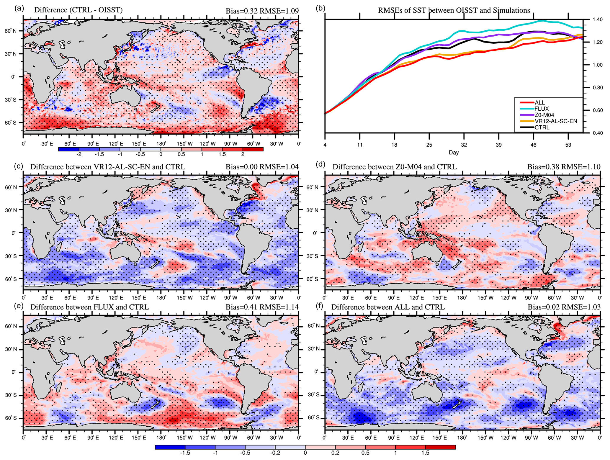
Figure 3 The 53 d average SST (^∘C) bias in CTRL (a; CTRL minus OISST), the time series of global-averaged RMSE (b), and the differences between VR12-AL-SC-EN (c) /Z0-M04 (d) /FLUX (e) /ALL (f), and CTRL in January–February 2017 (VR12-AL-SC-EN/Z0-M04/FLUX/ALL minus CTRL). The first 3 d of the simulation is discarded. The dotted areas are statistically significant at 95 % confidence level.

2.3.2 The Stokes–Coriolis force and associated entrainment

Because the Stokes drift velocity is an increment superimposed on the original current velocity, the Coriolis force and the Stoke drift together produce an additional so-called Stokes–Coriolis (SC) force (Hasselmann 1970); that is,

$$\begin{array}{}\text{(8)}& \text{SC Force}={\mathit{u}}_{\mathrm{s}}\left(z\right)\times f\mathit{z}.\end{array}$$

Here u_s(z) is the Stokes drift velocity vector, f is the Coriolis frequency, and z is the vertical unity vector. For consistency, the Stokes drift velocity is also included in advection terms of tracers (e.g., temperature, salinity) and convergence terms (Law-Chune and Aouf, 2018; Couvelard et al., 2020). And the free surface condition for barotropic mode is correspondingly modified to

$$\begin{array}{}\text{(9)}& {\displaystyle \frac{\partial \mathit{\eta }}{\partial t}}=-\mathrm{\nabla }{M}_{\mathrm{curr}}-\mathrm{\nabla }{M}_{\mathrm{st}},\end{array}$$

where η is surface elevation, and M_curr and M_st are the total vertical integral of the regular Eulerian current and the Stokes drift, respectively.

Figure 4 The same as Fig. 3 but for August–September 2018.

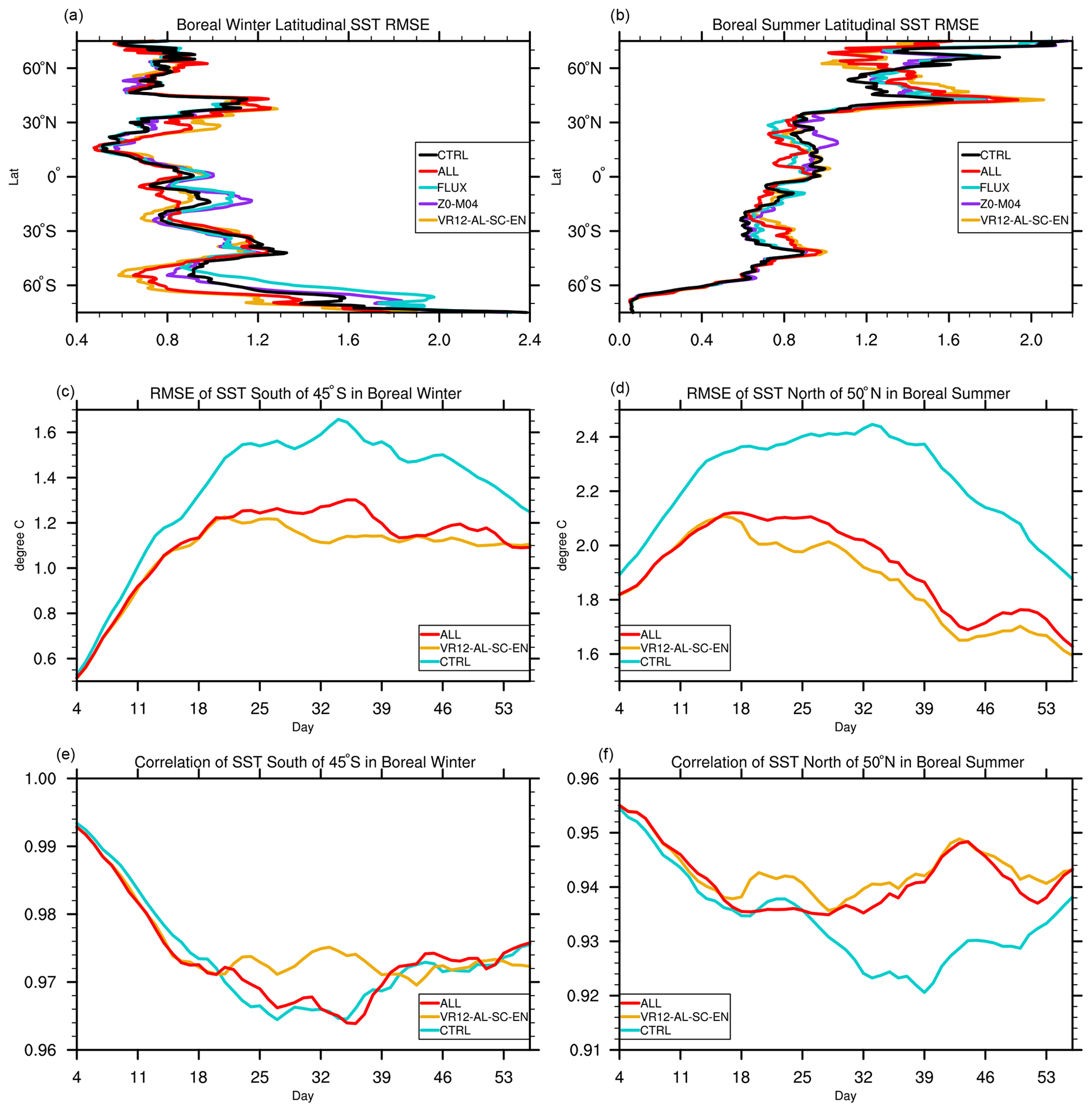
Figure 5 The 53 d averaged latitudinal distribution of SST root-mean-square errors (RMSE), time series of domain-averaged SST RMSE, and correlation coefficient: (a), (b) the latitudinal RMSE in boreal winter/summer compared with OISST; (c), (d) the time series of domain-averaged (0–360^∘ E, 45–78^∘ S/50–78^∘ N) SST RMSE in boreal winter/summer; (e), (f) the time series of domain-averaged (0–360^∘ E, 45–78^∘ S/50–78^∘ N) SST correlation coefficient in boreal winter/summer; differences of RMSE and correlation coefficient time series between VR12-AL-SC-EN/ALL and CTRL are statistically significant at 99 % confidence level, except those in Fig. e​​​​​​​.

To depict the entrainment below the ocean surface boundary layer induced by the Stokes drift, Li et al. (2016) suggested adding the square of the surface Stokes drift velocity (|u_s(0)|²) to the denominator of Eq. (7); that is,

$$\begin{array}{}\text{(10)}& R{i}_b\left(h\right)={\displaystyle \frac{gh[{\mathit{\rho }}_r-\mathit{\rho }(h\left)\right]}{{\mathit{\rho }}_{\mathrm{0}}[{\left|u_r-u\left(h\right)\right|}^{\mathrm{2}}+W^{\mathrm{2}}+\mathrm{|}{u}_{\mathrm{s}}(\mathrm{0}\left){\mathrm{|}}^{\mathrm{2}}\right]}}=R{i}_{\mathrm{cr}}.\end{array}$$

The boundary layer depth h in KPP from Eq. (10) is then enhanced due to the Stokes drift velocity.

2.4 The Stokes drift and sea surface current on air–sea fluxes

At the air–sea boundary layer, the momentum flux (τ), sensible heat flux (SH), and freshwater flux (E) are calculated as

$$\begin{array}{}\text{(11)}& {\displaystyle }\mathit{\tau }={\mathit{\rho }}_{\mathrm{a}}{C}_{\mathrm{d}}\left|\mathrm{\Delta }\mathit{V}\right|\mathrm{\Delta }\mathit{V},\text{(12)}& {\displaystyle }\mathrm{SH}={\mathit{\rho }}_{\mathrm{a}}{C}_{\mathrm{h}}\left|\mathrm{\Delta }\mathit{V}\right|\mathrm{\Delta }\mathit{\theta },\text{(13)}& {\displaystyle }E={\mathit{\rho }}_{\mathrm{a}}{C}_{\mathrm{e}}\left|\mathrm{\Delta }\mathit{V}\right|\mathrm{\Delta }q,\end{array}$$

where C_d, C_h, and C_e are surface exchange coefficients for momentum, sensible heat, and freshwater. ρ_a is air density. Δθ and Δq are potential temperature and humidity differences between air and sea, and ΔV is velocity of air relative to water flow.

In CFSv2.0, ΔV is set to be wind speed (U_wind). However, the effect of ocean surface current should not be ignored. Luo et al. (2005) first indicated that including ocean surface current (U_surf) improves estimates of τ and subsequent ocean response. Renault et al. (2016) further indicated that the improvements of τ by U_surf also fed back into the atmosphere. At present, $\mathrm{\Delta }\mathit{V}={\mathit{U}}_{\mathrm{wind}}-{\mathit{U}}_{\mathrm{surf}}$ is widely used in coupled ocean–atmosphere models (e.g., Hersbach and Bidlot, 2008; Takatama and Schneider, 2017​​​​​​​; Renault et al., 2021). Furthermore, Bao et al. (2019) indicated that as a part of the sea surface water movement with speed magnitude comparable to surface current in mid-to-high latitudes, the surface Stokes drift (u_s(0)) should also be included; that is,

$$\begin{array}{}\text{(14)}& \mathrm{\Delta }\mathit{V}={\mathit{U}}_{\mathrm{wind}}-{\mathit{U}}_{\mathrm{surf}}-{\mathit{u}}_{\mathrm{s}}\left(\mathrm{0}\right).\end{array}$$

To account for the effects of the surface currents and of the Stokes drift, Eq. (14) is used in the coupled experiments (Table 1). To complete the coupling, the corresponding modification of the tridiagonal matrix (Lemarié, 2015) has been implemented in CFSv2.0. Note that the direction of Stokes drift is generally consistent with 10 m wind (Fig. S1i and j in the Supplement), but the directions of surface current and 10 m wind are usually different due to the Coriolis effect (Fig. S1g and h). Consequently, the effects of U_surf and u_s(0) on ΔV depend on the angles between them and U_wind.

2.5 Parameterizations of momentum roughness

In CFSv2.0, the fluxes of momentum, heat, and freshwater are passed from atmosphere to ocean, and their estimate is critically important. The fluxes are in part determined by surface roughness length, which can be converted to surface exchange coefficients based on Monin–Obukhov similarity theory (Monin and Obukhov, 1954).

2.5.1 The momentum roughness length in GFS

In GFS, the momentum roughness length z₀ has two terms. The first term, z_ch, is parameterized by the Charnock relationship (Charnock, 1955), representing wave-resulted sea surface roughness, and the second term, z_vis, is the viscous contribution (Beljaars, 1994) for low winds and smooth surface; that is,

$$\begin{array}{}\text{(15)}& z_{\mathrm{0}}=z_{\mathrm{ch}}+z_{\mathrm{vis}}={\displaystyle \frac{C_{\mathrm{ch}}{u}_{\ast }^{\mathrm{2}}}{g}}+{\displaystyle \frac{\mathrm{0.11}\mathit{\nu }}{u_{\ast }}}.\end{array}$$

Here C_ch=0.014 is the constant Charnock parameter, and ν is the air kinematic viscosity. The relation of z₀ in GFS versus 10 m wind speed is shown in Fig. 2 (black line).

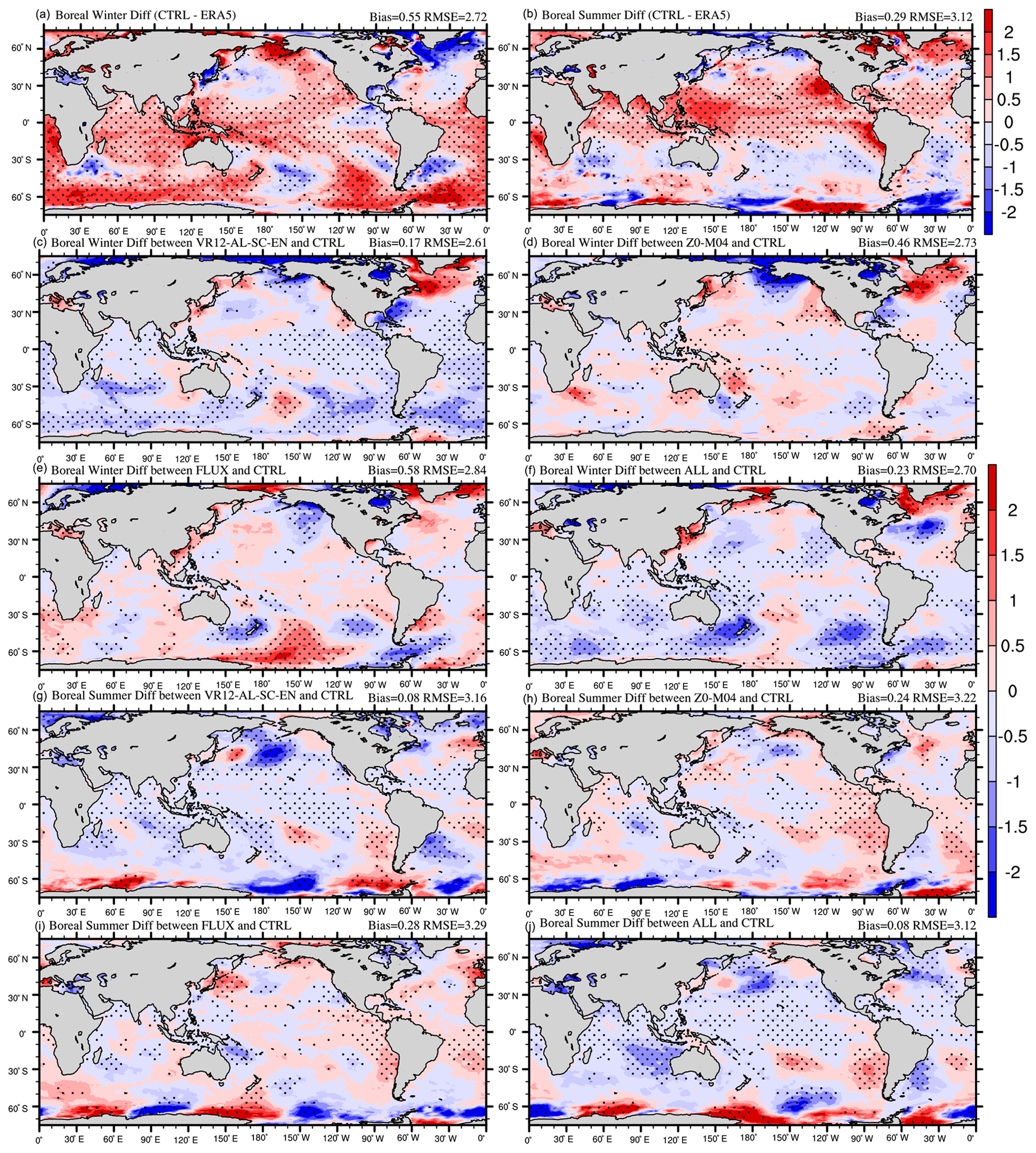
Figure 6 The 53 d average T02 (^∘C) bias in CTRL (a and b; CTRL minus ERA5), and the differences between VR12-AL-SC-EN (c and g) /Z0-M04 (d and h) /FLUX (e and i) /ALL (f and j) and CTRL (VR12-AL-SC-EN/Z0-M04/FLUX/ALL minus CTRL). The first 3 d of the simulation is discarded. The dotted areas are statistically significant at 95 % confidence level. Panels (a), (c), (d), (e), and (f) are for January–February 2017, and panels (b), (g), (h), (i), and (j) are for August–September 2018.

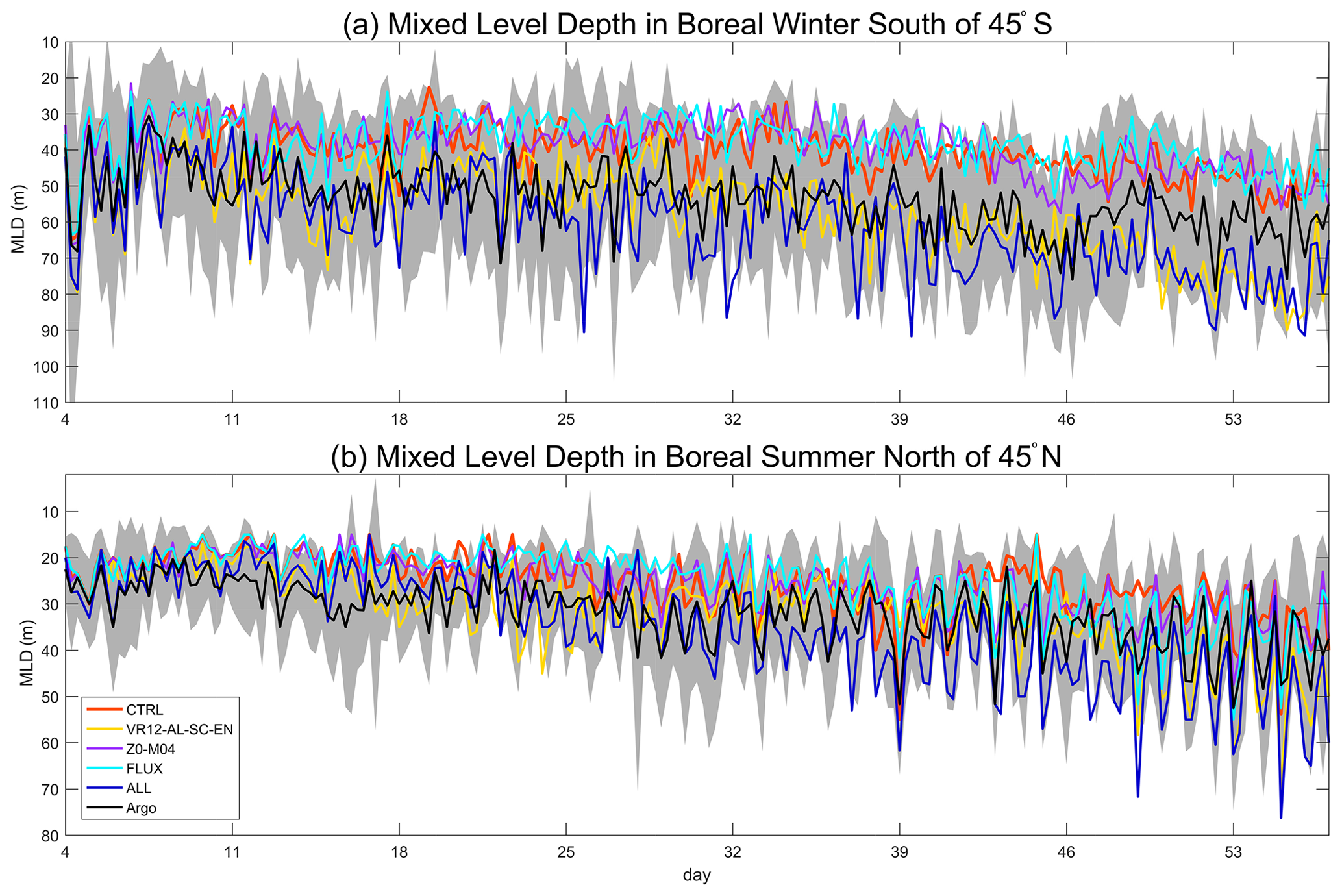
Figure 7 The 53 d time series of domain-averaged (0–360^∘ E, 45–78^∘ S/N) mixed layer depth (MLD, m) in boreal winter/summer: the difference between CTRL and VR12-AL-SC-EN/ALL passes the Student's t test at 99 % confidence level; the time intervals are 6 h; shaded areas indicate twice the standard deviations for Argo.

2.5.2 The Charnock relationship related to wave state

When ocean surface waves are explicitly considered, the Charnock parameter, C_ch, is not a constant (Janssen, 1989, 1991; Taylor and Yelland, 2001; Moon et al., 2004; Drennan et al., 2003, 2005). In the study, we adopt a method developed by Moon et al. (2004), which considered the surface roughness leveling off under extremely high wind speed (Powell et al., 2003; Donelan et al., 2004). Based on observations, Moon et al. (2004) proposed Eq. (16) to estimate the Charnock parameter by the wave age $\frac{c_{\mathrm{pi}}}{u_{\ast }}$ (c_pi is the peak phase speed of the dominant wind-forced waves) with constant values of a and b changing with 10 m wind speed every 5 m s⁻¹ in the range of 10 to 50 m s⁻¹.

$$\begin{array}{}\text{(16)}& C_{\mathrm{ch}}=a({\displaystyle \frac{c_{\mathrm{pi}}}{u_{\ast }}}{)}^b.\end{array}$$

To obtain continuous values of a and b, we derive a new relationship (Eq. 17 to estimate a and b from 10 m wind speed U₁₀ by fitting the values in Table 1 of Moon et al., 2004):

$$\begin{array}{ll}{\displaystyle }& {\displaystyle }a={\displaystyle \frac{\mathrm{1}}{\mathrm{0.1477}{U}_{\mathrm{10}}^{\mathrm{2}}-\mathrm{0.7395}{U}_{\mathrm{10}}-\mathrm{10.9995}}},\\ \text{(17)}& {\displaystyle }& {\displaystyle }b=\mathrm{1.5661}{E}^{-\mathrm{5}}{U}_{\mathrm{10}}^{\mathrm{3}}-\mathrm{0.002}{U}_{\mathrm{10}}^{\mathrm{2}}+\mathrm{0.1017}{U}_{\mathrm{10}}-\mathrm{1.6182}.\end{array}$$

Because the observations in Moon et al. (2004) were obtained under tropical cyclones, Eq. (17) is used for U₁₀>15 m s⁻¹, whereas the original Charnock relationship of the WW3 ST4 scheme (Janssen, 1989, 1991) is used for U₁₀≤15 m s⁻¹. The revised parameterization is called ST4-M04. Figure S2 in the Supplement shows the C_ch distribution obtained by Eqs. (16)–(17). In general small wind direction variations at low latitudes lead to large wave age and thus low C_ch. The situation is opposite at mid-to-high latitudes.

The relationships between z₀ and U₁₀ in GFS, WW3 ST4 scheme (Janssen, 1989, 1991), and ST4-M04 scheme are compared in Fig. 2. The z₀ in GFS increases relatively slowly with increasing wind speed (black). The value of z₀ from ST4 scheme (purple) increases rapidly with wind speed at high winds. In comparison, in ST4-M04 scheme (blue) the rapid increase in z₀ at high wind speed is obviously restrained, although the mean z₀ is slightly higher than that in GFS at wind speed >10 m s⁻¹ due to larger C_ch (>0.014 in Fig. S2). Furthermore, since the Charnock number is constant in GFS, the standard deviation (SD) of z₀ at a given wind speed is near zero. Since z₀ is determined only by wind-sea conditions in ST4 and ST4-M04 schemes, the SD at a given wind speed is mainly due to variations in wind fetch and development stage of sea state. The reduced SDs in ST4-M04 scheme, compared to ST4, imply less sensitivity of z₀ to fetch and sea state. Note that ST4-M04 is used in GFS, while z₀ in WW3 is still calculated by the ST4 source term to avoid affecting the balance of adjusted wind input and dissipation.

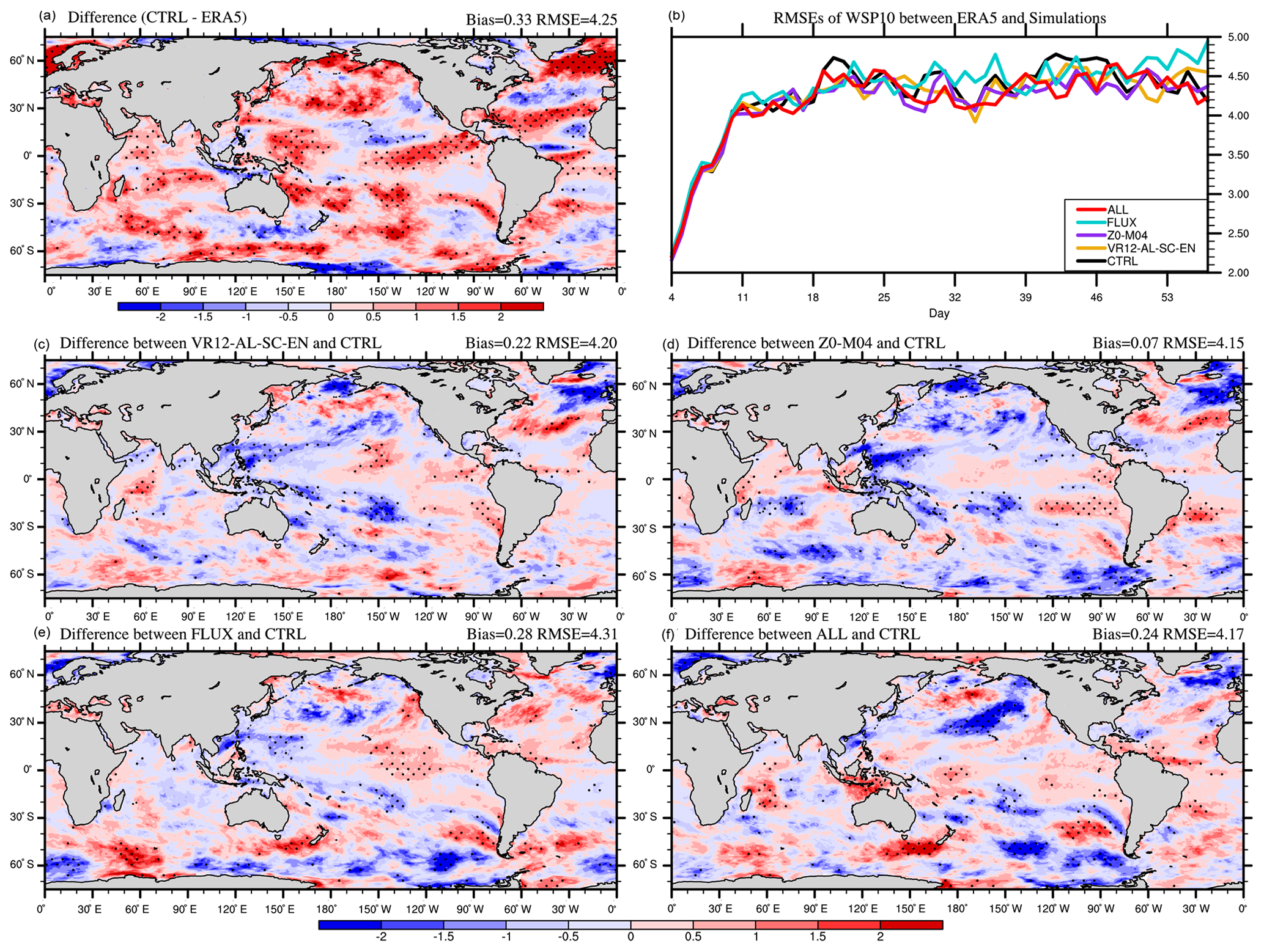
Figure 8 The 53 d average WSP10 (m s⁻¹) bias in CTRL (a; CTRL minus ERA5), the time series of global-averaged RMSE (b), and the differences between VR12-AL-SC-EN (c) /Z0-M04 (d) /FLUX (e) /ALL (f) and CTRL in January–February 2017 (VR12-AL-SC-EN/Z0-M04/FLUX/ALL minus CTRL). The first 3 d of the simulation is discarded. The dotted areas are statistically significant at 95 % confidence level.

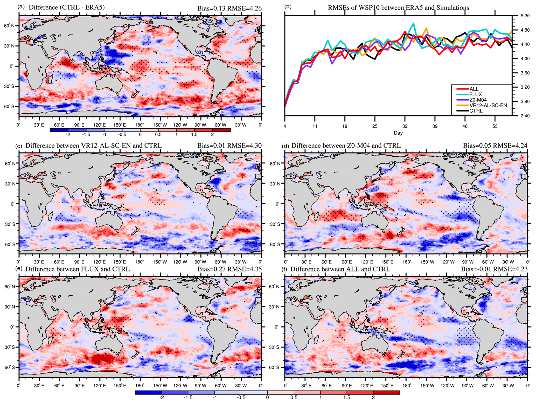
Figure 9 The same as Fig. 8 but for August–September 2018.

2.6 Set of experiments

A series of numerical experiments is conducted to evaluate the effects of the aforementioned wave-related processes on ocean and atmosphere in two 56 d periods, from 3 January to 28 February 2017​​​​​​​ and from 3 August to 28 September 2018 for boreal winter and boreal summer, respectively.

The reference experiment (CTRL) is a one-way coupled experiment, in which CFSv2.0 provides 10 m wind and surface current to WW3, whereas no variable is transferred from WW3 to CFSv2.0. The results of CFSv2.0 in CTRL are consistent with the corresponding CFS Reanalysis data (Saha et al., 2010). For each period, four sensitivity experiments are carried out (Table 1). Based on CTRL, the first is the VR12-AL-SC-EN experiment, in which the Langmuir mixing parameterization is used with the Stokes–Coriolis force and entrainment in MOM4. The second is the Z0-M04 experiment, in which the constant C_ch in GFS is replaced by C_ch from the WW3 ST4-M04 scheme. The effect of fluxes in GFS generated by ΔV (Eq. 14) is tested in the FLUX experiment. The last experiment is ALL, which includes all three parameterizations.

3 Data

Due to the availability of in situ and reanalysis data in the simulation periods, only sea surface temperature (SST), ocean subsurface temperature and salinity (T&S), 2 m air temperature (T02), 10 m wind speed (WSP10), and significant wave height (SWH) are used to evaluate the simulation results.

The daily-average satellite Optimum Interpolation SST (OISST) data are obtained from NOAA, with 0.25^∘ × 0.25^∘ resolution (Reynolds et al., 2007; https://www.ncdc.noaa.gov/oisst, last access: 20 January 2022). The global Argo observational profiles of T&S (Li et al., 2019) are from China Argo Real-time Data Center (http://www.argo.org.cn, last access: 20 January 2022). The ERA5 datasets of T02, WSP10, and SWH with a spatial resolution of 0.5^∘ are also used (Hersbach et al., 2020; https://cds.climate.copernicus.eu/cdsapp#!/dataset/reanalysis-era5-single-levels, last access: 20 January 2022), which assimilated huge amounts of historical data and thus provided reliable hourly estimates. Additionally, the WSP10 and SWH observations from the available National Data Buoy Center (NDBC) buoy data (https://www.ndbc.noaa.gov, last access: 20 January 2022) are used for comparison.

4 Experimental results

In this section, an evaluation of simulation results is presented. Comparisons are made between model results and observations or reanalysis data. The results in the first 3 d are excluded in the evaluation, since the wave influences are weak at the beginning. Compared with observations or ERA5, the general increase in the biases in all experiments is likely a drift from the initial conditions since no data are assimilated.

4.1 Sea surface temperature (SST) and 2 m air temperature (T02)

Figure 3a shows the spatial distribution of 53 d (day 4 to day 56) averaged SST biases in CTRL in boreal winter, defined as SST in CTRL minus OISST. The global mean SST bias is approximately 0.32 ^∘C, and the average RMSE is about 1.09 ^∘C from day 4 to day 56 in CTRL (Fig. 3a). The simulated SSTs are generally overestimated, and the large biases (>1.0 ^∘C) are mainly distributed in the Southern Ocean. In Fig. 3b, the global-averaged RMSEs of CTRL (black) increase with time in the first month and then gradually level off. Compared with CTRL, the RMSEs are reduced continuously in VR12-AL-SC-EN and ALL (yellow and red) but not in Z0-M04 and FLUX (purple and blue).

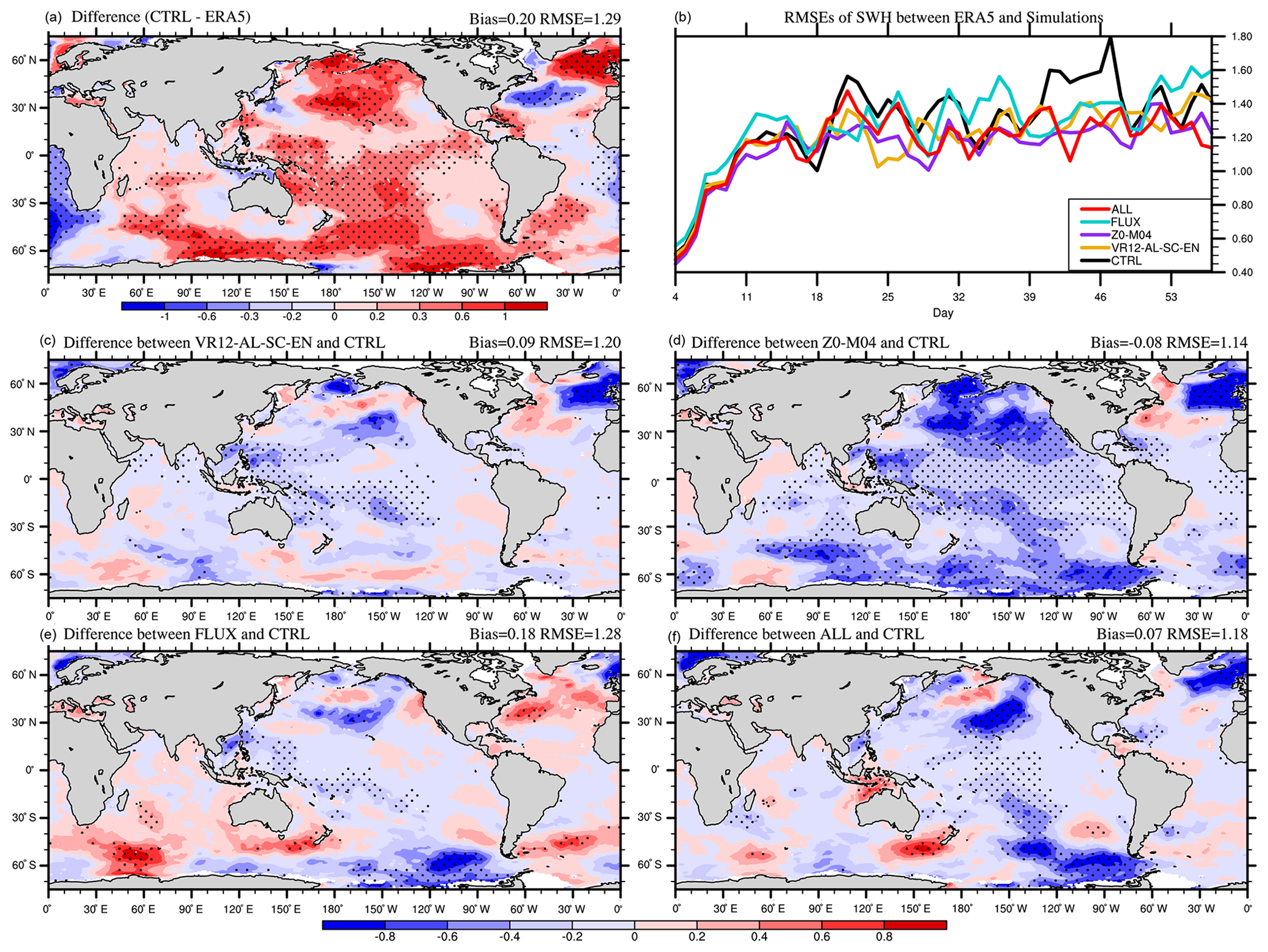
Figure 10 The 53 d average SWH (m) bias in CTRL (a; CTRL minus ERA5), the time series of global-averaged RMSE (b), and the differences between VR12-AL-SC-EN (c) /Z0-M04 (d) /FLUX (e) /ALL (f) and CTRL in January–February 2017 (VR12-AL-SC-EN/Z0-M04/FLUX/ALL minus CTRL). The first 3 d of the simulation is discarded. The dotted areas are statistically significant at 95 % confidence level.

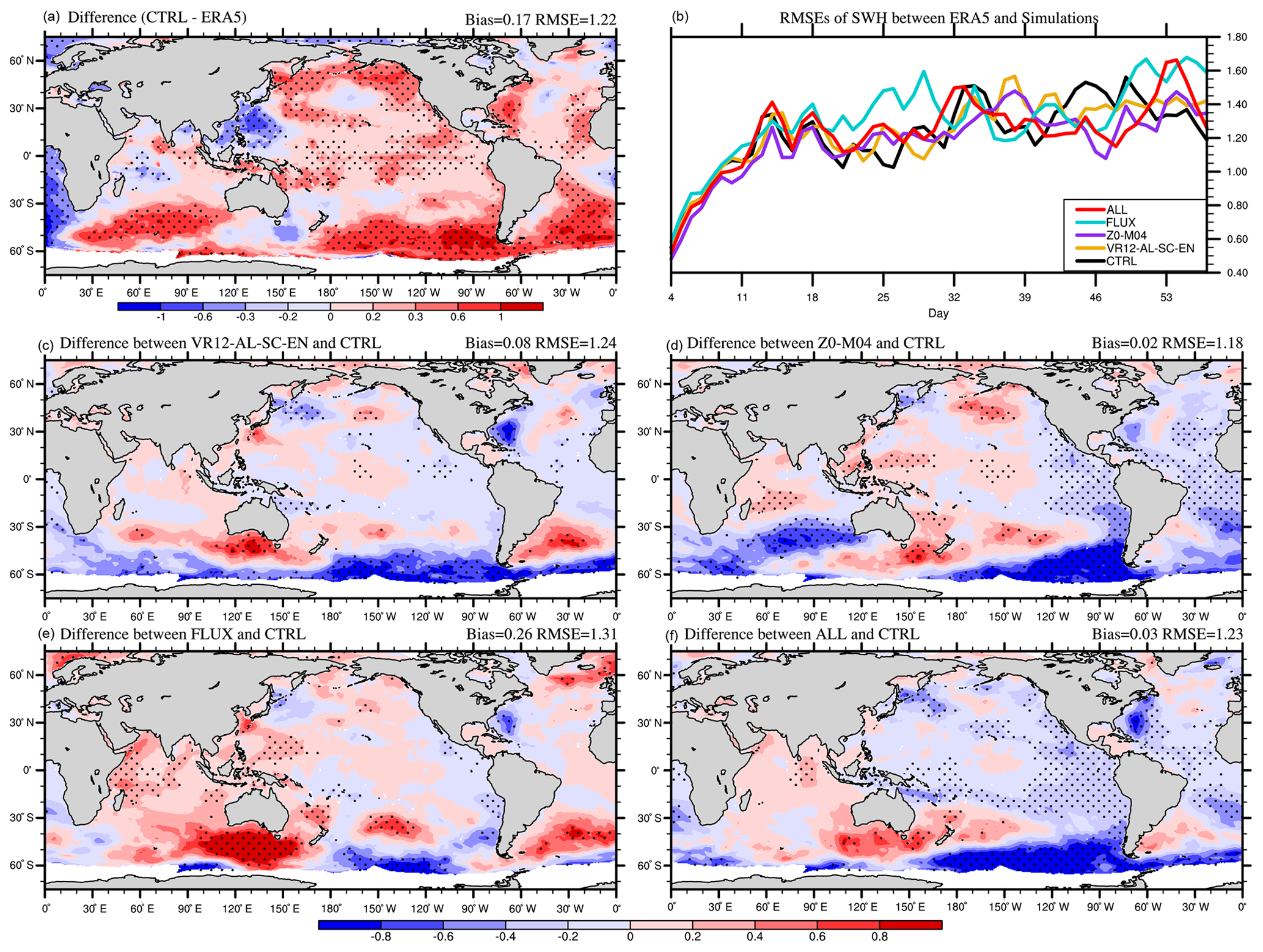
Figure 11 The same as Fig. 10 but for August–September 2018.

To understand the critical process responsible for the bias reduction in ALL, the SST differences are compared across all four experiments (Fig. 3c–f). Clearly, the difference in experiment VR12-AL-SC-EN is similar to that in ALL (Fig. 3c and f). The spatial correlation coefficient between the SST differences with CTRL of the two experiments (Fig. 3c and f) is 0.67, significant at 99 % confidence level, and the RMSEs of SST are not different significantly (red and yellow lines in Fig. 3b), indicating the Stokes drift-related parameterizations in VR12-AL-SC-EN mainly contribute to the SST positive bias reduction. This contrasts with Couvelard et al. (2020), where SST overestimations and MLD underestimations are reduced mainly due to the directly modified turbulence kinetic energy scheme. The global mean SST bias in ALL is 0.02 ^∘C with RMSE of 1.03 ^∘C, and in most areas the SST differences compared with CTRL are significant (P≤0.05) (dotted areas in Fig. 3f). Large SST improvements mainly appear in the Southern Ocean, with a regional RMSE decrease from 1.27 to 1.04 ^∘C south of 45^∘ S (Fig. 3f and red line in Fig. 5a). The reduction of overestimated SSTs in CTRL (red in Fig. 3a) is because the Stokes drift-related parameterizations in MOM4 inject turbulent kinetic energy into the ocean, which enhances vertical mixing and subsequently cools the surface waters (Belcher et al., 2012; Li et al., 2016). The modified roughness and relative velocity in Z0-M04 and FLUX also influence upper ocean mixing (Fig. 3d and e) via changing momentum flux and lead to generally warmer SSTs (purple and blue lines in Figs. 3b and 5a). The effect from Stokes drift-related ocean mixing parameterizations dominates SST changes in ALL.

In boreal summer, the global mean SST bias in CTRL is overestimated approximately 0.29 ^∘C, and the averaged RMSE from day 4 to day 56 is about 1.19 ^∘C. The overestimated SSTs (>1.0 ^∘C) mainly occur in the Northern Hemisphere (Fig. 4a). The global-averaged RMSEs are also generally lower in VR12-AL-SC-EN and ALL than in CTRL (Fig. 4b). The cooling effects in VR12-AL-SC-EN lead to a global mean bias of 0.06 ^∘C, and the large SST improvements mainly occur north of 50^∘ N (Fig. 4c and yellow line in Fig. 5b). The changes in SST in Z0-M04 and FLUX (Fig. 4d and e; purple and blue lines in Figs. 4b and 5b) are relatively small. The global mean bias in ALL is 0.04 ^∘C with an RMSE of 1.14 ^∘C (Fig. 4f).

As mentioned before, large improvements of overestimated SST mainly occur at mid-to-high latitudes in local summer. The time series of RMSEs and correlation coefficients of SST between model and observation in the region (0–360^∘ E, 45–78^∘ S in boreal winter and 0–360^∘ E, 50–78^∘ N in boreal summer) are shown in Fig. 5c–f. The RMSEs in CTRL (blue in Fig. 5c and d) increase in the first few weeks and then gradually decrease afterward. Compared with CTRL, RMSEs in VR12-AL-SC-EN (yellow) and ALL (red) are significantly (P≤0.01) reduced by about 0.3 ^∘C. The spatial correlation coefficients decrease with time but remain high (>0.90) for all experiments (Fig. 5e and f) with higher values in experiment VR12-AL-SC-EN (yellow).

We also compared T02 from experiments with ERA5 (Fig. 6). Warm biases of T02 appear in both winter and summer in CTRL (Fig. 6a and b). The changes in T02 in sensitivity experiments (Fig. 6c–j) are generally consistent with the changes in SST in the same experiments (Figs. 3 and 4). The correlation coefficients between the SST and the T02 changes for the ALL experiment in boreal winter and summer (Figs. 3f and 6f and 4f and 6j) are 0.61 and 0.53, respectively, significant at 99 % confidence level. In boreal winter, all wave-coupled experiments except FLUX reduce the T02 mean bias (Fig. 6c–f). VR12-AL-SC-EC has the largest T02 bias reduction compared with CTRL, from 0.55 to 0.17 ^∘C (Fig. 6c). In boreal summer, both VR12-AL-SC-EC and ALL have the largest T02 bias reduction, from 0.29 to 0.08 ^∘C (Fig. 6g and j). Noticeably, the improvements in RMSEs are not large for all experiments, because the improvements mainly occur in areas with overestimated temperature.

4.2 Mixed layer depth (MLD)

To further evaluate the direct effect of the wave-related processes on the upper ocean, we compare the MLD of all experiments with that estimated from Argo profiles in summer. The simulated T&S are interpolated onto the positions of Argo profiles at the nearest time. The MLD is estimated as the depth where the change of potential density reaches the value corresponding to a 0.2 ^∘C decrease in potential temperature with unchanged salinity from surface (de Boyer Montégut et al., 2004; Wang and Xu, 2018).

The time series of MLDs from numerical experiments and Argo south of 45^∘ S in boreal winter (north of 45^∘ N in boreal summer) are compared in Fig. 7a (b). The simulated MLDs are generally within the SD of Argo MLDs (shading in Fig. 7). In CTRL, the mean bias (CTRL minus Argo) with SD is −13.15 ± 7.82 m (−6.75 ± 5.29 m) in boreal winter (summer). The correlation coefficient of MLDs in CTRL with Argo MLDs is 0.55 (0.68) with P≤0.01, and the mean RMSE is 15.30 m (8.55 m) in boreal winter (summer). In ALL, the mean bias (ALL minus Argo) with SD is 7.70 ± 10.42 m (3.30 ± 7.78 m) in boreal winter (summer), and the correlation coefficient of MLDs enhances to 0.63 (0.78). The RMSE south of 45^∘ S decreases from 15.30 m in CTRL to 12.96 m in ALL. The RMSE north of 45^∘ N decreases from 6.71 in CTRL to 5.55 m in ALL in the first 6 weeks but the value increases in the last 2 weeks due to overestimation of MLDs. Compared with CTRL (orange in Fig. 7), VR12-AL-SC-EN (yellow) and ALL (dark blue) show significant improvements (P≤0.01) on the underestimated MLDs time series, whereas the MLDs difference between CTRL and Z0-M04 (purple)/FLUX (blue) is nonsignificant.

4.3 Wind speed at 10 m (WSP10) and significant wave height (SWH)

Compared with ERA5, the WSP10s in CTRL are generally overestimated in both winter and summer (Figs. 8a and 9a). The global averaged RMSEs of WSP10s in CTRL are 4.25 m s⁻¹ (4.26 m s⁻¹) in boreal winter (summer). The global averaged RMSEs of WSP10s in all experiments increase with time in the first 2 weeks and then gradually level off (Figs. 8b and 9b). The differences of RMSEs between CTRL and other experiments are tiny in the first 10 d, and afterwards the RMSEs in Z0-M04 and ALL (purple and red) become clearly smaller than in CTRL over most of the time.

The comparisons of the simulated SWHs in CTRL with the ERA5 also show that the SWHs are overestimated in both winter and summer (Figs. 10a and 11a). In boreal winter, the global mean SWH bias in CTRL is approximately 0.20 m with overestimates (>0.30 m) in the Pacific, the North Atlantic and the Southern Ocean (Fig. 10a), and the average RMSE is about 1.29 m. In boreal summer, the global mean bias in CTRL is approximately 0.17 m with 1.22 m RMSE (Fig. 11a). Similar to WSP10s, the RMSEs of SWHs also increase in the first 2 weeks and then gradually level off (Figs. 10b and 11b). The RMSEs in Z0-M04 and ALL (purple and red) are smaller than in CTRL over most of the time, consistent with changes in WSP10s. The correlation coefficients between changes in WSP10s and changes in SWHs in ALL are 0.77 and 0.73 in boreal winter and summer, respectively (Figs. 8f and 10f and 9f and 11f), significant at 99 % confidence level, indicating that the SWHs changes are closely related to changes in wind speeds.

In VR12-AL-SC-EN, the reduction of SST warm biases affects air temperature and stabilizes the marine atmospheric boundary layer (Sweet et al., 1981; O'Neill et al., 2003), and subsequently reduces WSP10s and SWHs with decreased global bias in boreal winter (Figs. 8c and 10c). In Z0-M04, the overestimated WSP10s and SWHs are also reduced (Figs. 8d and 10d) due to the larger z₀ with the ST4-M04 scheme at wind speed >10 m s⁻¹ (Fig. 2). The increase in z₀ enhances wind stress and momentum transferred into the ocean and therefore reduces surface winds (Pineau-Guillou et al., 2018; Sauvage et al., 2020) and consequently reduces SWHs. In FLUX (Figs. 8e and 10e), U_surf and u_s(0) decrease wind stress and momentum transfer when their directions are consistent with wind directions and vice versa (Hersbach and Bidlot, 2008; Renault et al., 2016). For instance, the angles between wind and current are relatively small (<90^∘) in the northeastern Pacific, reducing the wind stress and thus enhancing WSP10s (Fig. 8e). In contrast, the large angles (>90^∘) between the northwesterlies and the Kuroshio in the northwestern Pacific enhance wind stress, and decrease WSP10s (Fig. 8e). Consequently, improvements occur in areas with misalignment of winds and currents. With all combined effects, the biases of WSP10s and SWHs in ALL in most regions are decreased (Figs. 8f and 10f), with the reduced global RMSEs of 4.17 m s⁻¹ and 1.18 m, respectively. In boreal summer, the improvements of WSP10s and SWHs are relatively small in terms of global averaged RMSEs, because of smaller positive biases in CTRL (Figs. 9a and 11a). In ALL, the global averaged bias of WSP10s (SWHs) is −0.01 m s⁻¹ (0.03 m). The largest reduction primarily appears in the Southern Ocean (Figs. 9f and 11f) to improve the overestimated westerlies and SWHs in CTRL (Figs. 9a and 11a).

Previous studies indicated that ocean surface winds in ERA5 are underestimated in some regions (Belmonte Rivas and Stoffelen, 2019; Kalverla et al., 2020; Sharmar and Markina, 2020). To better demonstrate the effects of waves on WSP10s and SWHs, comparisons of WSP10s and SWHs with the NDBC buoy data are made (Table 2 and Fig. 12). The differences between sensitivity experiments and CTRL are all statistically significant at 95 % confidence level. Buoys are mainly located in the northeastern Pacific, the tropical Pacific, and the northwestern Atlantic oceans (Fig. S3), and buoy identifiers with total numbers, longitudes, and latitudes are listed in Table S3. The method from Hsu et al. (1994) is used to adjust wind speeds from buoy data to the reference height of 10 m.

Table 2 The 53 d mean bias with standard deviation (SD) and RMSE for WSP10 and SWH compared with NDBC buoy observation: the bias is calculated as simulation minus NDBC.

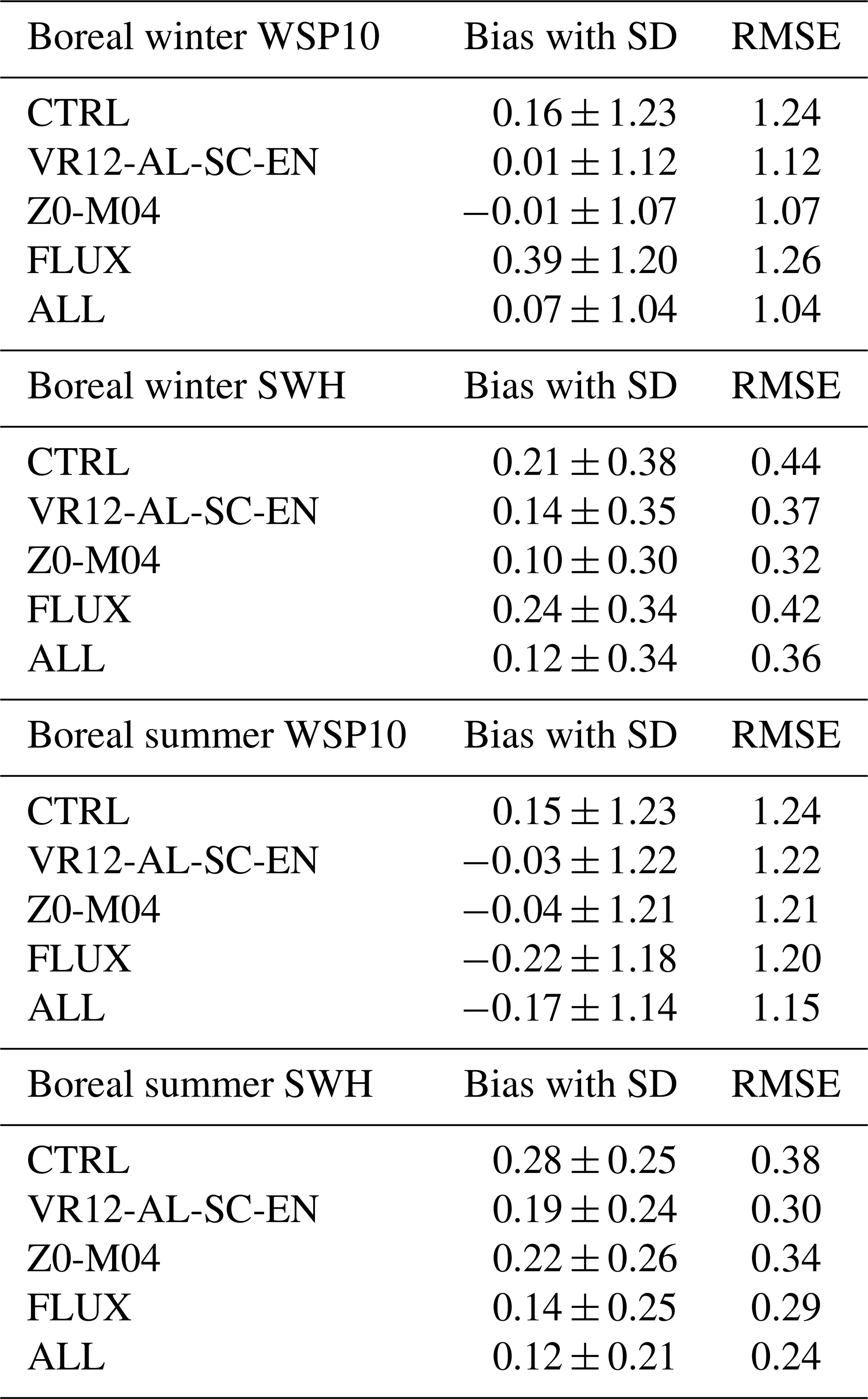
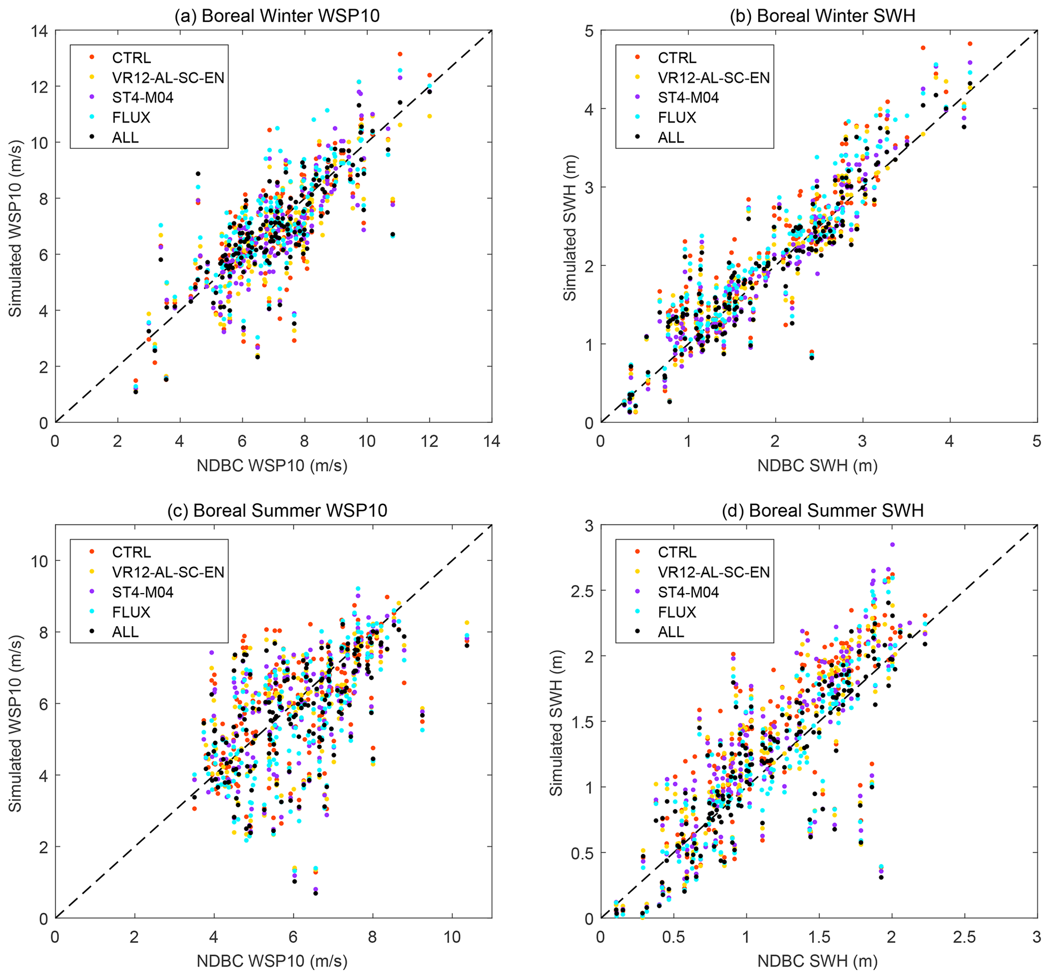
Figure 12 Scatterplots of simulated WSP10/SWH (y axis) vs. buoy WSP10/SWH (x axis): (a) the WSP10 in January–February 2017, (b) the SWH in January–February 2017, (c) the WSP10 in August–September 2018, and (d) the SWH in August–September 2018. The dotted line is y=x. The corresponding mean biases with standard deviations and RMSEs for every experiment are shown in Table 2.

Compared to the NDBC data, the WSP10s and the SWHs in CTRL are generally overestimated in both winter and summer with positive mean biases (Table 2 and Fig. 12). The reduction of mean biases appears in all experiments except FLUX in boreal winter. The wave-related processes are most effective in areas with positive biases, consistent with previous comparisons with ERA5. In boreal winter, the angles between winds and currents are small. The wind stresses are then reduced in FLUX, and the WSP10s are enhanced, so the positive bias is further enhanced. The improvements in ALL are generally the largest (Table 2), with the WSP10s RMSE of 1.04 m s⁻¹ (1.15 m s⁻¹) and the SWHs RMSE of 0.36 m (0.24 m) in boreal winter (summer). As shown in Fig. 12, with the increase in WSP10s and SWHs, the reduction of overestimation in ALL compared with CTRL is more prominent.

5 Summary and discussion

To investigate the individual role played by wave-related processes on the atmosphere and ocean interface in a coupled global atmosphere–ocean–wave modeling system on an intraseasonal scale, we implement version 5.16 of WW3 into CFSv2.0 over the domain 78^∘ S–78^∘ N, using the C-Coupler2. In this coupled system, the WW3 is forced by 10 m wind and surface current generated in CFSv2.0. The Stokes drift-related Langmuir mixing, the Stokes–Coriolis force and entrainment in ocean, air–sea fluxes modified by surface current and the Stokes drift, and momentum roughness length (z₀) are considered separately, and the results of sensitivity experiments are compared against in situ buoys, satellite measurements, and ERA5 reanalysis. The effects of waves on intraseasonal prediction are examined in two 56 d cases, one for boreal winter and the other one for boreal summer.

The following key results are found:

1. Overestimated SST, T02, and underestimated MLD in the mid-to-high latitudes in CFSv2.0 are significantly improved, particularly in local summer. Langmuir turbulence, Stokes–Coriolis force and entrainment in VR12-AL-SC-EN lead to enhanced vertical mixing. The enhanced vertical mixing changes the temperature structure in the upper ocean and further affects air temperature. In boreal winter, the regional RMSE of SST (T02) in the Southern Ocean decreases from 1.27 (1.93) in the CTRL experiment to 1.04 (1.67) ^∘C in the ALL experiment. In boreal summer, the effect is weaker because of the relatively smaller ocean areas in the mid-to-high latitudes of the Northern Hemisphere.

2. In general, all wave-related processes reduce biases for WSP10s and SWHs, particularly in regions where WSP10s and SWHs were overestimated. The decreased SSTs in VR12-AL-SC-EN stabilize the marine atmospheric boundary layer and lead to weakened WSP10s and SWHs. The modified roughness in Z0-M04 generally enhances momentum transfer into the ocean, and so decreases WSP10s and SWHs. The relative wind–wave-current speed in FLUX also affects wind stress and further influences WSP10s and SWHs. Compared with NDBC buoy observations and ERA5, the ALL experiment shows significant improvements.

In addition to the variables mentioned before, the changes in simulated enthalpy fluxes are also compared, which mainly depend on the WSP10s changes. However, the wave-related effects on enthalpy fluxes are nonsignificant for the 2-month simulation, so the results are not shown.

The wave-related parameterizations used in the study mainly improve model biases at mid-to-high latitudes, and SST biases in tropical oceans are only slightly improved (Figs. 3 and 4). Breivik et al. (2015) improved SST as well as subsurface temperature simulations in Nucleus for European Modelling of the Ocean (NEMO) with parameterizations including the wave-related Charnock parameter, modification of water-side stress with wind input and wave dissipation, wave dissipation-related turbulent kinetic energy flux, and the Stokes–Coriolis force. Based on a global NEMO–WW3 coupled framework, Couvelard et al. (2020) modified the Charnock parameter, the Stokes drift-related forces and the Langmuir cell with misalignment of winds and waves, the oceanic surface momentum flux, and the turbulence kinetic energy to reduce SST and MLD biases. In addition, sea spray can enhance air–sea heat fluxes in the tropics (Andreas et al., 2008, 2015). We will consider more processes in future studies.

Different parameterizations for the same wave-related process also deserve discussion. For ocean surface roughness, the most classic parameterizations are those developed by Janssen (1989, 1991), Taylor and Yelland (2001), and Drennan et al. (2003). The method by Taylor and Yelland (2001) requires the peak wavelength for the total spectrum, whereas that by Drennan et al. (2003) only requires the peak of wind-sea waves. This difference leads to the fact that the former is more suitable for a mixed sea state, while the latter is more suitable for a young sea state (Drennan et al., 2005). And the effect of Janssen's parameterization (Janssen, 1989, 1991) is similar to that of Drennan et al. (2003), since it is also based on the wind-sea conditions (Shimura et al., 2017).

Our case studies indicate that significant biases in the coupled system remain, probably owing to inaccuracy of the coarse resolution, absence of a coupled wave–ice module, and deficiency of initial fields. In addition, every individual model component could be further improved via new parameter settings or updated parametrization schemes. All these aspects will need to be considered for improving our coupled system.