From emission scenarios to spatially resolved projections with a chain of computationally efficient emulators: coupling of MAGICC (v7.5.1) and MESMER (v0.8.3)

Producing targeted climate information at the local scale, including major sources of climate change projection uncertainty for diverse emissions scenarios, is essential to support climate change mitigation and adaptation efforts. Here, we present the first chain of computationally efficient Earth system model (ESM) emulators that allow for the translation of any greenhouse gas emission pathway into spatially resolved annual mean temperature anomaly field time series, accounting for both forced climate response and natural variability uncertainty at the local scale. By combining the global mean, emissions-driven emulator MAGICC with the spatially resolved emulator MESMER, ESM-specific and constrained probabilistic emulated ensembles can be derived. This emulator chain can hence build on and extend large multi-ESM ensembles such as the ones produced within the sixth phase of the Coupled Model Intercomparison Project (CMIP6). The main extensions are threefold. (i) A more thorough sampling of the forced climate response and the natural variability uncertainty is possible, with millions of emulated realizations being readily created. (ii) The same uncertainty space can be sampled for any emission pathway, which is not the case in CMIP6, where only a limited number of scenarios have been explored and some of the most societally relevant strong mitigation scenarios have been run by only a small number of ESMs. (iii) Other lines of evidence to constrain future projections, including observational constraints, can be introduced, which helps to refine projected ranges beyond the multi-ESM ensembles' estimates. In addition to presenting results from the coupled MAGICC–MESMER emulator chain, we carry out an extensive validation of MESMER, which is trained on and applied to multiple emission pathways for the first time in this study. By coupling MAGICC and MESMER, we pave the way for rapid assessments of any emission pathway's regional climate change consequences and the associated uncertainties.

1 Introduction

Earth system models (ESMs) are the primary tools to study the impact of greenhouse gas emissions on regional climate change (IPCC, 2013, 2021). While the insights they provide are invaluable to advance our understanding of the coupled Earth system to external influences, their projections are affected by three major sources of uncertainty: (i) internal variability uncertainty, i.e., unforced natural climate variability; (ii) forced climate response uncertainty, i.e., uncertainty in the response of the climate system to both forced natural (solar and volcanic) and anthropogenic (greenhouse gases, aerosols, land use change, etc.) influences; and (iii) emission scenario uncertainty, i.e., which emission pathway the world chooses (Hawkins and Sutton, 2009; Lehner et al., 2020). Each of these uncertainty classes again encompass a myriad of different contributions to the total uncertainty, e.g., carbon cycle uncertainty, aerosol forcing uncertainty, and climate sensitivity uncertainty are all captured within the climate response uncertainty in the above categorization. Due to their high computational cost, ESMs can only sparsely explore the full uncertainty phase space.

This sparse exploration is problematic since targeted climate information accounting for all major sources of climate change uncertainty is urgently needed, especially because both Earth's climate (IPCC, 2013, 2018, 2021) and the future emission pathway the world's nations have pledged to follow (CAT, 2019, 2021a, b) are changing rapidly. When assessing the implications of a large number of emission pathways for future climate, it is neither computationally feasible nor efficient to create full ESM ensembles for each emission pathway, especially ESM ensembles which thoroughly sample the natural variability and climate response uncertainty space. Instead, computationally inexpensive ESM emulators can be useful tools to provide targeted climate information for a few key variables, such as surface air temperature.

Figure 1 Illustration of the MAGICC–MESMER emulator chain. The sequence of the analysis starts from either an emission or a concentration scenario, as highlighted in panel (a) for the CO₂ concentration time series of the historical time period and two Shared Socioeconomic Pathway (SSP) scenarios (O'Neill et al., 2017), namely SSP1-1.9 and SSP3-7.0. The probabilistic global mean temperature change distributions – whose medians and 90 % ranges (5th–95th percentile) are shown in panel (b) – consist of realizations that are a combination of the scenario-specific forced global warming from MAGICC and emulated global natural variability from MESMER. Based on this information, MESMER can derive the associated spatially resolved temperature change distributions, with the maps shown in panel (c) representing the 5th percentile, the median, and the 95th percentile (each map trio from bottom to top) for 2014 (first column of maps), for 2050 for both SSP scenarios (second column of maps), and for 2100 for both SSP scenarios (third column of maps).

Here, we present the first chain of computationally efficient ESM emulators able to translate user-defined emission or concentration scenarios into spatially and temporally resolved temperature anomalies with respect to a pre-industrial baseline accounting for all major sources of climate change uncertainty (Fig. 1). In this study, the global MAGICC emulator (Meinshausen et al., 2009, 2011, 2020) is used to turn greenhouse gas concentration pathways into constrained probabilistic forced global temperature change time series by taking multiple lines of evidence into account. These are then translated into temperature anomaly field time series, accounting for both regional forced climate response and internal natural variability uncertainty, with the spatially resolved MESMER emulator (Beusch et al., 2020a), calibrated on a set of ESMs from the sixth phase of the Coupled Model Intercomparison Project (CMIP6; Eyring et al., 2016) ensemble.

Figure 2 Visualization of the cumulative contribution of different uncertainty sources accounted for in the MAGICC–MESMER emulator chain with time series for a single grid point in eastern North America and with maps of example realizations for the year 2030 for the low-emission scenario SSP1-1.9. The example emulations shown in the maps are also depicted in the grid-point-level time series by using the colors displayed on top of the maps. Note that whenever several colors are depicted on top of a single map, the associated emulations all exhibit an identical temperature change trajectory. Hence, the individual example emulations fully overlap both in the map and in the time series plot. Light blue markers are employed to indicate the year 2030 in the time series plots and to show which location the time series belong to on the maps. From top to bottom, the rows exhibit an increasing reflection of uncertainties. Panel (a) accounts for no uncertainty since a single MAGICC forced global warming time series is combined with a single MESMER forced response pattern, meaning that all emulations are identical. Panel (b) accounts for the uncertainty in the global response by combining all of MAGICC's forced global warming time series with a single MESMER forced response pattern. In the time series plot, the solid black line indicates the median of the temperature change distribution for that grid point, and the gray shading shows the 90 % range (5th–95th percentile). Panel (c) adds uncertainty in the regional response by combining all of MAGICC's forced global warming time series with all of MESMER's forced response patterns. Panel (d) adds natural internal variability provided by MESMER on top of the forced response patterns.

Figure 2 illustrates how the different sources of uncertainty accounted for in the MAGICC–MESMER chain accumulate at the local scale by presenting time series for a single grid point in eastern North America and maps of example realizations in 2030 for a low-emission scenario. In the most basic setup of the MAGICC–MESMER chain, a single forced global mean temperature change time series can be coupled to a single set of local forced response parameters, resulting in a single spatially resolved forced warming time series (Fig. 2a). When accounting for global climate response uncertainty by using MAGICC's probabilistic distribution of forced global mean temperature time series in combination with the single local forced response parameter set, a range of realizations are obtained but they all share the same spatial pattern (Fig. 2b). Different spatial patterns become available once the uncertainty in the regional forced response is included and the forced global temperature time series are combined with each of the different available ESM-specific local forced response parameter sets (Fig. 2c). The last source of uncertainty is ESM-specific natural climate variability, which is added on top of the local forced response patterns (Fig. 2d). In this low-emission scenario, natural variability accounts for roughly half of the uncertainty at the local scale even at the end of the 21st century. For a high-emission scenario, the overall spread at the end of the century in terms of regional forced response would increase, and thus natural variability would be less important compared to the other sources of uncertainty.

While this study is, to our knowledge, the first to combine all of these uncertainties in a single emulator chain, rich background literature exists around emulating each individual uncertainty aspect. The uncertainty in the global climate response to greenhouse gas emissions is modeled by a variety of global emulators, which usually have a physical core and use different statistical approaches during calibration (Nicholls et al., 2021c). The uncertainty in the local forced response to global temperature is most frequently accounted for through different flavors of pattern scaling (Tebaldi and Arblaster, 2014; Lynch et al., 2017; Beusch et al., 2020a). The last element of our emulation chain, local-scale natural variability, has been stochastically created through re-sampling of either individual temperature field realizations (Alexeeff et al., 2018) or of principal components with perturbed phases (Link et al., 2019), and by sampling from autoregressive processes with spatially correlated innovation terms (Beusch et al., 2020a). Additionally, there are two studies that directly translate emissions into spatially resolved temperature change realizations (Goodwin et al., 2020; Yuan et al., 2021). However, both of the available approaches do not account for all major sources of uncertainty. Goodwin et al. (2020) combine the global emulator WASP with a pattern scaling approach to obtain probabilistic mean warming realizations but do not account for internal climate variability. Yuan et al. (2021), on the other hand, use a statistical emulator calibrated on a single ESM to create spatially resolved temperature realizations directly from CO₂ equivalence concentrations and thus neither account for forced climate response uncertainty nor uncertainty in the representation of unforced natural climate variability.

2 Data

2.1 ESM data

We use climate information from 25 ESMs participating in the Scenario Model Intercomparison Project (ScenarioMIP; O'Neill et al., 2016) of CMIP6 (Eyring et al., 2016) listed in Appendix Table A1. While our ESM ensemble does not contain all of the ESMs available within CMIP6, it does cover a wide range of temperature realizations and is broadly representative of the overall warming spread and the relative fraction of simulations available for each scenario.

Data from 1850–2100 are employed, covering the historical time period (1850–2014) and the ScenarioMIP's future (2015–2100) emission and land use change scenarios, i.e., the Shared Socioeconomic Pathways (SSPs) SSP1-1.9, SSP1-2.6, SSP4-3.4, SSP5-3.4-over, SSP2-4.5, SSP4-6.0, SSP3-7.0, and SSP5-8.5. In this study, a special focus is set on SSP1-1.9, the most ambitious mitigation scenario of CMIP6, and SSP3-7.0, a physically plausible high-end emission scenario (Hausfather and Peters, 2020).

We primarily employ annual 2 m air temperature (T) data, but ocean heat uptake (OHU) is additionally used for some analyses. Both variables are re-gridded onto a common 2.5^∘ × 2.5^∘ spatial grid according to Brunner et al. (2020a). Anomalies with respect to 1850–1900 are obtained at the grid-point level and used for all analyses.

Regional averages refer to area-weighted averages, and regional land averages refer to area-weighted and land-fraction-weighted averages. Grid cells with more than one-third land fraction according to the land–sea mask of the regionmask package v0.8.0 (Hauser et al., 2021b) are considered to be land grid points. The global land average does not include Antarctica as no emulations are created for Antarctica. The eastern North America region frequently employed throughout this study is one of the updated Intergovernmental Panel on Climate Change (IPCC) climate reference regions (Iturbide et al., 2020) and is extracted from the gridded fields with the help of the regionmask package v0.8.0 (Hauser et al., 2021b).

2.2 Observational data

To calibrate MESMER, a proxy for volcanic activity is needed in addition to temperature data (Beusch et al., 2020a). Here, we use the globally averaged stratospheric aerosol optical depth time series employed in the recently published Sixth Assessment Report of the IPCC (Forster et al., 2021; Smith et al., 2021b) for this purpose. The time series is available in monthly resolution (Smith et al., 2021a), and thus annual averages need to be created before using it.

For a qualitative visual validation of the MAGICC–MESMER emulations, annual blended temperature anomalies from the Berkeley Earth data set are employed (Rohde and Hausfather, 2020), which consist of land and sea ice 2 m air temperature anomalies and ocean surface temperature anomalies. They are interpolated onto the same spatial grid as the ESM data, also following the approach described in Brunner et al. (2020a). To account for differences in the global average of blended temperature anomalies and 2 m air temperature anomalies, the observational global blended averages ΔT^glob,blend are transformed into 2 m air global averages ΔT^glob,air at every point in time t via $\mathrm{\Delta }{T}_t^{\mathrm{glob},\mathrm{air}}=\mathrm{1.098}\cdot \mathrm{\Delta }{T}_t^{\mathrm{glob},\mathrm{blend}}-\mathrm{0.001}$ ^∘C, a relationship derived by Beusch et al. (2020b) based on CMIP6 data. Additionally, the observational data need to be shifted from their native 1951–1980 baseline to the 1850–1900 baseline employed within this study. However, during the 1850–1900 time period, the observational data are not spatially complete and the quality of the available data is lower. Hence, the MAGICC–MESMER emulated regional median warming between the 1850–1900 baseline and the native baseline of the observational data is added to the observational data as a constant offset during plotting.

3 Methods

3.1 MAGICC (v7.5.1)

MAGICC is a reduced complexity climate model that calculates – among other quantities – forced global warming and global ocean heat uptake. Its hemispherically resolved, multi-layer upwelling–entrainment–diffusion ocean and climate cores (based on the energy balance equation with state- and forcing-dependent climate sensitivity) are described in Meinshausen et al. (2011) and Meinshausen et al. (2020). It also includes representations of the carbon cycle, non-CO₂ greenhouse gas cycles, and the relationship between aerosol precursor species emissions and aerosol effective radiative forcing (Meinshausen et al., 2011, 2020), alongside a parameterization of the response of permafrost to global heating (Schneider von Deimling et al., 2012).

The MAGICC output employed throughout this paper is the same as presented in Nicholls et al. (2020) and Nicholls et al. (2021c). We use simulations driven by greenhouse gas concentrations, following the CMIP6 ScenarioMIP approach (O'Neill et al., 2016). A slightly wider output temperature distribution would be achieved if MAGICC were run in an emissions-driven mode instead (Nicholls et al., 2021c).

3.2 MESMER (v0.8.3)

3.2.1 Default configuration: local temperature anomalies as a function of global temperature anomalies

The MESMER emulator was introduced in Beusch et al. (2020a) to emulate multi-ESM initial-condition ensembles for a specific emission pathway in a spatially resolved manner. This first MESMER configuration has thus far been successfully applied to emulate temperature anomalies for the highest-emission scenarios of both the CMIP5 (Beusch et al., 2020a) and the CMIP6 (Beusch et al., 2020b) ensembles.

MESMER is an ESM-specific emulator that needs to be calibrated for each emulated ESM separately to capture the unique characteristics of that ESM, both in terms of local forced warming and local variability around the forced warming (Beusch et al., 2020a). Within MESMER, local temperature anomalies ΔT for a specific climate model “m” at every point in space “s” and time “t” are emulated as follows:

$$\begin{array}{}\text{(1)}& \begin{array}{rl}\mathrm{\Delta }{T}_{\mathrm{m},\mathrm{s},\mathrm{t}}& =f\left(\mathrm{\Delta }{T}_{\mathrm{m},\mathrm{t}}^{\mathrm{glob}}\right)+{\mathit{\eta }}_{\mathrm{m},\mathrm{s},\mathrm{t}}={\mathit{\beta }}_{\mathrm{m},\mathrm{s}}^{\mathrm{fr}}\cdot \mathrm{\Delta }{T}_{\mathrm{m},\mathrm{t}}^{\mathrm{glob},\mathrm{fr}}\\ & +{\mathit{\beta }}_{\mathrm{m},\mathrm{s}}^{\mathrm{iv}}\cdot \mathrm{\Delta }{T}_{\mathrm{m},\mathrm{t}}^{\mathrm{glob},\mathrm{iv}}+{\mathit{\beta }}_{\mathrm{m},\mathrm{s}}^{\mathrm{intercept}}+{\mathit{\eta }}_{\mathrm{m},\mathrm{s},\mathrm{t}}.\end{array}\end{array}$$

The local temperature anomaly is a direct function of global mean temperature change ΔT^glob and a spatiotemporally correlated noise term η. At every point in space, a multiple linear regression is employed to relate ΔT^glob information to local temperature anomalies. Forced global temperature change ΔT^glob,fr and internal global temperature variability ΔT^glob,iv serve as predictors. The associated regression coefficients are β^fr and β^iv. β^intercept constitutes the intercept term. ΔT^glob,fr is obtained by first applying locally weighted scatterplot smoothing (LOWESS) to the ΔT^glob time series and subsequently adding volcanic spikes to the smooth forced temperature time series via a linear regression of the global temperature anomaly residuals to stratospheric aerosol optical depth. The remaining internal global variability ΔT^glob,iv and the residual local variability η are both modeled as autoregressive processes. For η, spatially correlated innovation terms are drawn to account for local to regional cross-correlations between grid points. Beusch et al. (2020a) describe the full algorithm and additionally carry out a thorough evaluation of the resulting emulations. In short, their evaluation highlights that MESMER reliably emulates grid-point-level forced warming and internal climate variability. However, they also show that MESMER's emulations are increasingly under-dispersive for larger regional averages since MESMER's local residual variability module reduces the magnitude of the empirical covariance between grid cells as a function of their geographical distance. At the global land level, MESMER emulations become reliable again, due to the global-scale variability captured through the ${\mathit{\beta }}_{\mathrm{m},\mathrm{s}}^{\mathrm{iv}}\cdot \mathrm{\Delta }{T}_{\mathrm{m},\mathrm{t}}^{\mathrm{glob},\mathrm{iv}}$ term.

In this work, MESMER is for the first time trained on and applied to the full range of emission scenarios covered within the CMIP6 ScenarioMIP projections instead of a single emission pathway. The main additional assumption when extending MESMER from emulating a single emission pathway to emulating a range of scenarios is that the estimated parameters are scenario-independent. This assumption of universal scenario applicability of the calibrated parameters is also regularly made in the well-established pattern scaling literature (Tebaldi and Arblaster, 2014), although care is nonetheless required, particularly for strong mitigation scenarios (Goodwin et al., 2020).

To obtain robust MESMER parameter estimates for each ESM, MESMER is trained on all available ensemble members of each available scenario and equal weight is given to each scenario. The scenarios employed for training are – subject to availability – SSP5-8.5, SSP3-7.0, SSP4-6.0, SSP2-4.5, SSP5-3.4-over, SSP4-3.4, SSP1-2.6, SSP1-1.9, and the historical scenario. Note that we consider the historical time period as its own scenario during the MESMER training. Since projections for different SSPs usually branch from the same historical members, the historical years would receive more weight if the historical and the future time period were concatenated during training.

Many ESMs have a different number of ensemble members (n_e) for each scenario, and the scenarios (historical and projections) have a different number of time steps (n_t), resulting in a different number of samples ($n_{\mathrm{s}}=n_{\mathrm{e}}\cdot n_{\mathrm{t}}$) per scenario. Therefore, when estimating the coefficients of the multiple linear regression, all simulations from all scenarios are pooled and each sample (e.g., the temperature anomaly for a specific location, year, and scenario) is weighted by $\mathrm{1}/n_{\mathrm{s}}$, i.e., by the inverse number of samples available for the respective scenario. The same approach is applied when estimating the empirical spatial covariance matrix of the residual local variability.

For the autoregressive processes, the coefficients are determined for each ensemble member individually and are subsequently averaged for each scenario before averaging across all scenarios. For the autoregressive process describing the global variability, the order of the process must additionally be selected before the parameters are fit. The order is first chosen for each ensemble member individually based on the Bayesian information criterion and then the median order is identified for each scenario. Lastly, the median order over all scenarios is selected to describe the global variability of the ESM at hand.

The ESM-specific forced global warming time series for each scenario is obtained by using data solely from that scenario, since the forced global warming module relies on a simple statistical smoothing and volcanic spikes approach (see Beusch et al., 2020a, for details). To facilitate the task of the forced global warming module, it operates directly on the average global warming across all ensemble members for a given ESM and scenario rather than on individual ensemble members.

3.2.2 Additional predictors configuration: local temperature anomalies as a function of global temperature anomalies and global ocean heat uptake

To account for potential nonlinearities in the climate system (Mitchell, 2003) and for changing forced response warming patterns when moving from a transient to an equilibrium climate (King et al., 2020), we introduce two additional predictors into the grid-point-level multiple linear regressions of MESMER (Eq. 1): (i) squared forced global temperature change (ΔT^glob,fr)² is used to represent nonlinear feedbacks, and (ii) the forced trend in global ocean heat uptake ΔOHU^glob,fr is used as a proxy for how close the climate system is to equilibrium. ΔOHU^glob,fr is obtained with the same LOWESS approach used to derive ΔT^glob,fr, but no volcanic spikes are added as they are already accounted for in the global temperature response. Hence, the grid-point-level temperature anomalies are emulated as follows:

$$\begin{array}{}\text{(2)}& \begin{array}{rl}\mathrm{\Delta }{T}_{\mathrm{m},\mathrm{s},\mathrm{t}}& ={\mathit{\beta }}_{\mathrm{m},\mathrm{s}}^{\mathrm{fr}}\cdot \mathrm{\Delta }{T}_{\mathrm{m},\mathrm{t}}^{\mathrm{glob},\mathrm{fr}}+{\mathit{\beta }}_{\mathrm{m},\mathrm{s}}^{\mathrm{fr}\mathrm{2}}\cdot (\mathrm{\Delta }{T}_{\mathrm{m},\mathrm{t}}^{\mathrm{glob},\mathrm{fr}}{)}^{\mathrm{2}}\\ & +{\mathit{\beta }}_{\mathrm{m},\mathrm{s}}^{\mathrm{fr},\mathrm{ohu}}\cdot \mathrm{\Delta }{\mathrm{OHU}}_{\mathrm{m},\mathrm{t}}^{\mathrm{glob},\mathrm{fr}}+{\mathit{\beta }}_{\mathrm{m},\mathrm{s}}^{\mathrm{iv}}\cdot \mathrm{\Delta }{T}_{\mathrm{m},\mathrm{t}}^{\mathrm{glob},\mathrm{iv}}\\ & +{\mathit{\beta }}_{\mathrm{m},\mathrm{s}}^{\mathrm{intercept}}+{\mathit{\eta }}_{\mathrm{m},\mathrm{s},\mathrm{t}},\end{array}\end{array}$$

where β^fr2 and β^fr,ohu are the newly introduced regression coefficients.

3.2.3 Evaluating both MESMER configurations

Before continuing with the methods, we evaluate the two proposed MESMER configurations. Specifically, we assess whether the additional predictors configuration offers considerable benefits over the default configuration. When analyzing climate information, it is often helpful to distinguish between forced response and natural variability. Here, we evaluate both MESMER configurations in terms of their performance in emulating single ESMs with respect to these two quantities. The two can be separated in a straightforward fashion within the additive MESMER framework (Eqs. 1 and 2).

The forced local temperature anomaly ΔT^fr of the default MESMER configuration consists of the following terms:

$$\begin{array}{}\text{(3)}& \mathrm{\Delta }{T}_{\mathrm{m},\mathrm{s},\mathrm{t}}^{\mathrm{fr}}={\mathit{\beta }}_{\mathrm{m},\mathrm{s}}^{\mathrm{fr}}\cdot \mathrm{\Delta }{T}_{\mathrm{m},\mathrm{t}}^{\mathrm{glob},\mathrm{fr}}+{\mathit{\beta }}_{\mathrm{m},\mathrm{s}}^{\mathrm{intercept}}.\end{array}$$

In the additional predictors configuration of MESMER, the contribution of the additional predictors enters the forced local temperature anomaly too, resulting in the following equation:

$$\begin{array}{}\text{(4)}& \begin{array}{rl}\mathrm{\Delta }{T}_{\mathrm{m},\mathrm{s},\mathrm{t}}^{\mathrm{fr}}& ={\mathit{\beta }}_{\mathrm{m},\mathrm{s}}^{\mathrm{fr}}\cdot \mathrm{\Delta }{T}_{\mathrm{m},\mathrm{t}}^{\mathrm{glob},\mathrm{fr}}+{\mathit{\beta }}_{\mathrm{m},\mathrm{s}}^{\mathrm{fr}\mathrm{2}}\cdot (\mathrm{\Delta }{T}_{\mathrm{m},\mathrm{t}}^{\mathrm{glob},\mathrm{fr}}{)}^{\mathrm{2}}\\ & +{\mathit{\beta }}_{\mathrm{m},\mathrm{s}}^{\mathrm{fr},\mathrm{ohu}}\cdot \mathrm{\Delta }{\mathrm{OHU}}_{\mathrm{m},\mathrm{t}}^{\mathrm{glob},\mathrm{fr}}+{\mathit{\beta }}_{\mathrm{m},\mathrm{s}}^{\mathrm{intercept}}.\end{array}\end{array}$$

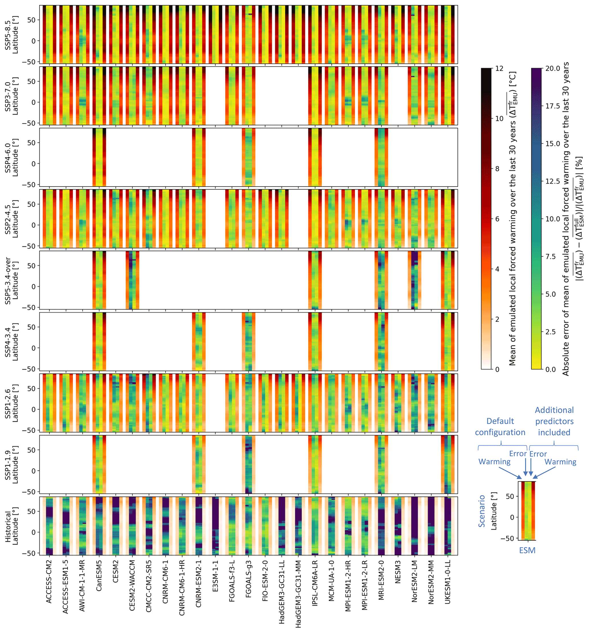
Figure 3 Latitudinally averaged grid-point-level mean of emulated local forced warming and performance with respect to ESM simulations for both MESMER configurations over the last 30 years of each scenario. The error shown here represents the absolute deviation between the mean of the emulated forced warming and the mean temperature anomaly value across all available ESM initial-condition members for the scenario at hand and is normalized by the absolute value of the mean of the emulated forced warming.

Figure 3 visualizes the latitudinally averaged mean of the local forced warming over the last 30 years for each individual ESM and scenario for both MESMER configurations. For a given scenario, the ESMs' latitudinal patterns exhibit considerable differences. For example, the magnitude of the Arctic amplification (Serreze and Barry, 2011) clearly differs between the ESMs. These regional differences are additionally visualized in maps for select high- and low-emission scenarios for each ESM in the Supplement (Figs. S1–S5). Overall, the patterns of forced warming are very similar in the default and additional predictors configurations (Fig. 3) and inter-ESM differences are considerably larger than MESMER inter-configuration differences.

Nevertheless, with the additional predictors configuration, consistent but small improvements are achieved for most ESMs (Fig. 3). The magnitude of the improvements depends on the ESM, the scenario, and the latitude. The improvements mostly occur in the highest-emission scenario (SSP5-8.5) and in the strong mitigation scenarios (SSP5-3.4-over, SSP1-2.6, and SSP1-1.9). This is an expected consequence of the additional predictors targeting nonlinearities and the transition to an equilibrium climate.

Overall, the performance is excellent for both MESMER configurations (Fig. 3): the latitudinally averaged absolute error with respect to the local warming signal rarely reaches 10 % in the future projections. The SSP1 scenarios have a tendency for higher percentage errors because of their lower overall forced warming signal. This is amplified in the historical period, since its low regional warming leads to small absolute deviations, translating into large percentage errors. In the Supplement (Figs. S1–S5), error maps can be found that further highlight regional differences in the errors for select high- and low-emission scenarios.

Sensitivity experiments are additionally carried out to quantify the impact on emulation performance when using a reduced number of scenarios during training. For MESMER's default configuration, a generally very similar, although slightly reduced, performance is achieved by only training on a single high-emission (SSP5-8.5) and low-emission (SSP1-2.6) scenario (Fig. S6). If only a single future scenario and the historical time period are used for training, a high-emission future scenario results in a better overall performance. This is because training on a low-emission scenario requires MESMER to extrapolate to warm climates when emulating higher-emission scenarios. Overall, the SSP5-8.5-trained default MESMER configuration often performs comparably to MESMER trained on all scenarios but experiences minor performance reductions in strong mitigation scenarios whose climate moves towards equilibrium conditions. The SSP1-2.6-trained emulator, on the other hand, struggles to emulate high-emission scenarios. Hence, for MESMER's default configuration even a single (high-emission) scenario largely suffices to emulate a wide range of different emission pathways as long as their emissions do not exceed the ones used for training. The best emulation performance across all scenarios is, however, achieved if both high- and low-emission scenarios are included in the training.

If the additional predictors configuration of MESMER is applied instead, it is more important that at least one high-emission scenario and one low-emission scenario are available during training because training on a single emission pathway leads to overfitting on the scenario type and thus poor emulation skill in other scenarios (Fig. S7). This mainly occurs because the cross-correlations between the three predictors ($\mathrm{\Delta }{T}_{\mathrm{m},\mathrm{t}}^{\mathrm{glob},\mathrm{fr}}$,$(\mathrm{\Delta }{T}_{\mathrm{m},\mathrm{t}}^{\mathrm{glob},\mathrm{fr}}{)}^{\mathrm{2}}$, and $\mathrm{\Delta }{\mathrm{OHU}}_{\mathrm{m},\mathrm{t}}^{\mathrm{glob},\mathrm{fr}}$) are fundamentally different in the high-emission transient climate change scenarios compared to the low-emission equilibrium-approaching scenarios.

After considering the forced response in detail, we now turn our attention to the local temperature variability for MESMER trained on all available scenarios. The ESM-specific emulated local temperature variability around the forced warming consists of the combination between the local response to the global variability and the residual local variability for both MESMER configurations:

$$\begin{array}{}\text{(5)}& \mathrm{\Delta }{T}_{\mathrm{m},\mathrm{s},\mathrm{t}}^{\mathrm{iv}}={\mathit{\beta }}_{\mathrm{m},\mathrm{s}}^{\mathrm{iv}}\cdot \mathrm{\Delta }{T}_{\mathrm{m},\mathrm{t}}^{\mathrm{glob},\mathrm{iv}}+{\mathit{\eta }}_{\mathrm{m},\mathrm{s},\mathrm{t}}.\end{array}$$

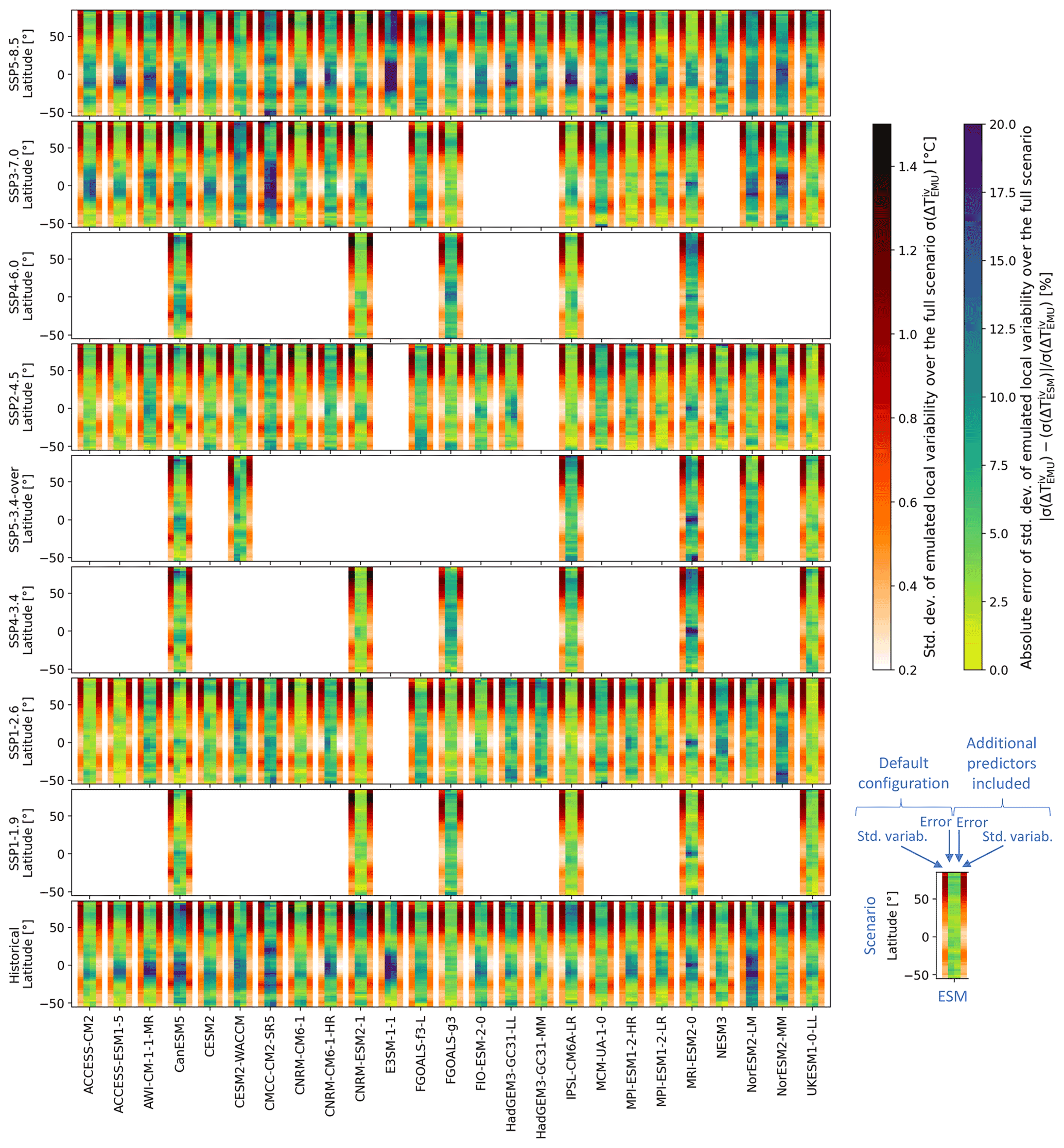
Figure 4 Latitudinally averaged grid-point-level standard deviation of emulated local variability and performance with respect to ESM simulations for both MESMER configurations over the full scenario period. The standard deviation of the emulated local variability is computed based on 600 variability emulations for each ESM. To obtain local variability from ESM simulations, the emulated local forced warming is subtracted from every ESM simulation. Subsequently, the standard deviation of these estimates of ESM simulations' local variability is computed while employing all ESM initial-condition ensemble members available for the scenario at hand. The error shown here represents the absolute deviation between the standard deviation of the emulated variability and the standard deviation of the ESMs' variability normalized by the standard deviation of the emulated variability.

Figure 4 shows the latitudinally averaged standard deviation of the emulated local variability analogously to Fig. 3 for each ESM and scenario available for that ESM. However, the standard deviations are computed over the full scenario length instead of only over the last 30 years to obtain more robust estimates. Additionally, the standard deviation of the emulated variability is identical for every scenario since no scenario dependence is integrated in the variability emulation. Differences in the error between different scenarios for individual ESMs hence solely occur because the ESMs' variability differs from simulation to simulation.

Generally, the emulated variability is smallest in the tropics and largest in the northern high latitudes, but considerable inter-ESM differences in the magnitude and spatial distribution exist (Fig. 4). In the Supplement Figs. S8–S12, spatially resolved maps of the standard deviation of the emulated local variability are shown that further highlight region-specific characteristics. MESMER inter-configuration differences are minimal in terms of improvements with respect to capturing the characteristics of the local variability of the actual ESM simulations (Fig. 4). However, the spatially resolved maps can help pinpoint differences in the errors of the two configurations in some regions (Figs. S8–S12).

The percentage errors in the emulated local variability (Fig. 4) are generally a bit larger than the forced local warming ones (Fig. 3). In part, the larger errors are caused by the fact that percentage differences are considered and that standard deviation of local variability is mostly a small quantity. This impression is reinforced by the fact that the largest percentage differences occur most often in the low-variability tropics. A possible physical explanation of the remaining errors is revealed by consulting maps of the error in the standard deviation (Figs. S8–S12). For certain ESMs and regions, the standard deviations are overestimated in the high-end scenario but underestimated in the low-end scenario (or the other way round), indicative of changes in local variability across climate states (Olonscheck and Notz, 2017), which are not accounted for in either MESMER configuration. In line with this finding, the highest deviations are generally observed for SSP5-8.5, which experiences the most extreme climatic change and thus also the largest changes in variability (Fig. 4). Given that SSP5-8.5 is designed to represent an unlikely high-risk future (Hausfather and Peters, 2020), one could justify excluding it from the local variability training to further improve the local variability emulations for the other scenarios. However, since the absolute differences in standard deviations are nevertheless rather small, we continue to use all scenarios for training.

This detailed MESMER evaluation reveals that the additional predictors bring systematic but small improvements. The main forced warming signal can already be successfully extracted based on forced global temperature change alone and local variability is generally emulated similarly well in both MESMER configurations. In the following, we thus use the default MESMER configuration instead of the additional predictors configuration. This minimizes the risk of poorly calibrated parameters when only a limited number of scenarios are available for training in which different predictors are strongly correlated.

3.3 Coupling MAGICC and MESMER

After determining the MESMER configuration to use throughout the rest of the paper, we now describe the employed MAGICC–MESMER coupling approach. MAGICC and MESMER are calibrated individually before using them jointly to create ensembles of spatially resolved emulations. In the coupled MAGICC–MESMER emulation mode, MESMER's own statistical estimates of ΔT^glob,fr in Eq. (1) are replaced with MAGICC's ΔT^glob,fr estimates (Sect. 3.2.1), making it possible to also provide spatially resolved emulations for emission scenarios which were not available during the MESMER training.

3.3.1 ESM-specific emulations

When emulating a specific ESM with MAGICC, a single forced global temperature anomaly ΔT^glob,fr time series is obtained for every emission scenario. Here, we employ ESM-specific MAGICC output published as part of the Reduced Complexity Model Intercomparison Project (RCMIP) Phase 1 (Nicholls et al., 2020) for two ESMs, CanESM5 and CNRM-CM6-1. Note that this output was generated with MAGICC v7.1.0-beta but that very similar results would be obtained with MAGICC v7.5.1, which is employed throughout all other parts of our study.

To obtain full global realizations ΔT^glob for these ESMs, the stochastically generated, ESM-specific global variability of MESMER ΔT^glob,iv is added to MAGICC's ESM-specific ΔT^glob,fr time series. For this study, 600 ΔT^glob,iv emulations are created with MESMER for each ESM. Hence, the MAGICC–MESMER ΔT^glob ensemble contains 600 realizations per ESM.

The spatially resolved forced warming fields ΔT^fr are obtained by combining MAGICC's ΔT^glob,fr time series with the associated ESM's local forced response parameters provided by MESMER (Eq. 3). The resulting ΔT^fr field time series is combined with 600 local variability emulations ΔT^iv for that ESM provided by MESMER (Eq. 5), leading to a 600-member ESM-specific MAGICC–MESMER ensemble of ΔT (Eq. 1).

The ESM-specific MAGICC–MESMER ensembles can be regarded as a direct approximation of very large ESM initial-condition ensembles (Deser et al., 2012, 2020), which can be provided at a negligible computational cost for any emission scenario of interest.

3.3.2 Globally constrained probabilistic emulations

To derive trustworthy probabilistic climate projections that thoroughly sample the climate response and natural variability uncertainty space for any emission scenario, observational constraints are often required. At each point of the MAGICC–MESMER emulation chain, an observational constraint could theoretically be introduced.

Several studies employing fundamentally different approaches have all demonstrated that the CMIP6 ESMs which exhibit the strongest future forced global warming are not consistent with observationally constrained forced global warming estimates (Forster et al., 2020; Beusch et al., 2020b; Brunner et al., 2020b; Tokarska et al., 2020; Nicholls et al., 2021c; Ribes et al., 2021). However, in terms of regional forced warming response to the global forced warming, i.e., in terms of regionally averaged ${\mathit{\beta }}_{\mathrm{m},\mathrm{s}}^{\mathrm{fr}}$ (see Eq. 1), most CMIP6 ESMs perform in an observationally consistent manner in most regions (Beusch et al., 2020b). Therefore, the MAGICC–MESMER constrained probabilistic projections are constrained solely at the global level and span the full regional ESM response uncertainty in this study.

The probabilistic MAGICC output used in this study follows the HadCRUT5 (Morice et al., 2021) calibration of MAGICC presented in Nicholls et al. (2021c) and consists of 600 forced global temperature change ΔT^glob,fr time series per scenario. It is assumed that global- and regional-scale performance are sufficiently decoupled to allow for combining MAGICC's probabilistic output with each of MESMER's ESM-specific local parameter sets. This assumption is supported by Beusch et al. (2020b), who demonstrate that there is no direct relation between an ESM's performance skill for global-scale forced warming response to emissions and regional-scale forced warming response to forced global warming. Hence, similar to the ESM-specific emulation approach, a full initial-condition ensemble is created for each combination of the 600 ΔT^glob,fr time series with the 25 ESM-specific parameter sets. For the global temperature realizations ΔT^glob, this means that each of the 600 MAGICC ΔT^glob,fr time series are combined with 600 global variability ΔT^glob,iv realizations of 25 ESMs, resulting in a total number of 9 million ΔT^glob realizations. For the local temperature anomaly field realizations ΔT, each of MAGICC's ΔT^glob,fr time series is combined with the ESM-specific local parameter sets of MESMER (Eq. 1). This results in 600 local forced temperature change ΔT^fr field time series for each ESM-specific parameter set (Eq. 3). Each of these local forced temperature field time series is subsequently combined with 600 local variability ΔT^iv realizations from MESMER (Eq. 5), yielding 600 different initial-condition ensembles with 600 members each (Eq. 1). Thus, 360 000 probabilistic ΔT realizations are contributed from each set of ESM-specific local parameters, and the full probabilistic ensemble contains 9 million emulations.

The complete sampling approach we employ here ensures a thorough sampling of the full uncertainty space but may quickly lead to computer memory issues. Alternatively, a broad – albeit sparser – sampling of the full climate response and natural variability uncertainty space could also be achieved by randomly combining single MAGICC time series with single ESM-specific parameter sets.

4 Results

4.1 ESM-specific temperature projections

To illustrate the MAGICC–MESMER chain's ability to capture the distinct behavior of individual ESMs in its ESM-specific configuration, we approximate the behavior of two example ESMs, CanESM5 and CNRM-CM6-1, for two example scenarios, SSP3-7.0 and SSP1-1.9 (Fig. 5). In both scenarios, the emulations serve to fill the gaps in the natural variability uncertainty space by successfully capturing the characteristic ESM-dependent forced warming and climate variability around that warming for the different spatial scales. The increasing magnitude of natural variability for smaller spatial scales results in an increasing overlap between the temperature anomaly distributions spanned by the two ESMs. In the low-emission scenario, the emulations additionally fill a gap in the climate response uncertainty space as no SSP1-1.9 simulations are available for CNRM-CM6-1. Hence, in this configuration, our emulator chain approximates the full climate change uncertainty phase space spanned by the considered ESMs since it can create very large emulated initial-condition ensembles for any given scenario.

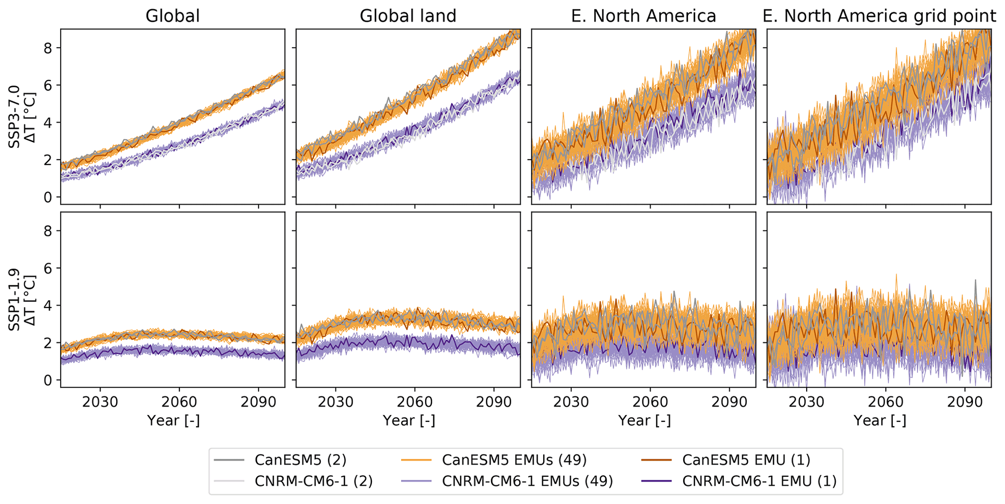
Figure 5 Temperature anomaly time series of ESM-specific MAGICC–MESMER emulations (in color) and actual ESM simulations (in gray) for CanESM5 and CNRM-CM6-1 averaged across different spatial scales: global, global land, eastern North America, and a single grid point within eastern North America for a high-emission (SSP3-7.0) and a low-emission (SSP1-1.9) scenario. For illustrative purposes, 50 out of the 600 available emulations are shown for both ESMs in color, and a single emulation is highlighted in a darker color. For the ESMs, two initial-condition ensemble members are shown for each scenario for which simulations are available.

It should be noted that the success of these ESM-specific emulations is strongly dependent on MAGICC's ability to match a given ESM's behavior over a range of scenarios. While we satisfactorily emulate the example ESMs shown here, there are other ESMs that are captured less accurately by MAGICC in this emulation mode (see Nicholls et al., 2020). On the other hand, the regional features of single ESMs given the forced global warming trajectories are generally well captured by MESMER (Sect. 3.2.3). Overall, in the context of ESM-specific emulation, more work on emulating ESMs' forced global temperature change is required compared to the relative success seen in emulating an ESM's natural variability and regional response to forced global warming.

4.2 Globally constrained probabilistic temperature projections

When sampling the full globally constrained climate response and internal variability uncertainty space with the probabilistic MAGICC–MESMER ensemble, the emulations no longer coincide with individual ESM simulations (Fig. 6). Instead, the globally constrained emulated ensemble encompasses a smaller range of temperature anomalies than the raw CMIP6 ensemble and also samples this space much more thoroughly with 9 million emulations. This thorough sampling means that even extreme quantiles at individual grid cells can be statistically robustly estimated in any year. An additional advantage with respect to the CMIP6 ensemble is that the same forced climate response and natural variability uncertainty space can be sampled for each scenario, whereas there are strong differences in the number of ESMs providing simulations for each scenario and in the number of available simulations of a single ESM for a specific scenario. This is especially relevant because SSP1-1.9, which is of great interest for society as it comes closest to the 1.5 ^∘C Paris Agreement temperature limit (UNFCCC, 2015), is one of the scenarios that has only been run by a rather small and warm sub-selection of ESMs. In our CMIP6 ensemble, only six ESMs provide SSP1-1.9 simulations, two of which warm unrealistically fast during the historical period in terms of global mean and continue to do so in the future (see, e.g., Tokarska et al., 2020; Beusch et al., 2020b). The global warming of these two ESM simulations is clearly incompatible with the globally constrained emulated ensemble (Fig. 6). The two ESMs' global and global land mean temperature anomalies are almost constantly above the 95th percentile of the emulated ensemble. At the regional and grid-point level, the constrained ensemble also warms distinctly less than these high-warming simulations, but the larger internal variability results in a partial overlap between those ESMs' realizations and the climate change uncertainty space (5th–95th percentile) of the emulated ensemble.

Figure 6 Temperature anomaly projection distributions for the emulated globally constrained probabilistic MAGICC–MESMER ensembles and actual ESM simulations averaged across different spatial scales: global, global land, eastern North America, and a single grid point within eastern North America for a high-emission (SSP3-7.0) and low-emission (SSP1-1.9) scenario. For the MAGICC–MESMER ensemble, the median and the 90 % range (5th–95th percentile) of the temperature anomaly distribution are shown in color. For the ESMs, a single simulation per available ESM for that emission pathway is shown in gray.

Figure 7 Temperature anomaly distribution for the emulated globally constrained probabilistic MAGICC–MESMER ensemble, actual CMIP6 simulations, and observations averaged across different spatial scales: global, global land, eastern North America, and a single grid point within eastern North America for the period covered by observations, i.e., the historical time period extended with the middle of the road future scenario (SSP2-4.5). For the MAGICC–MESMER ensemble, the median and the 90 % range (5th–95th percentile) of the temperature anomaly distribution is shown in color. For the ESMs, a single simulation per available ESM for that scenario is depicted in gray. The observations are shown in black.

To qualitatively validate the probabilistic MAGICC–MESMER ensemble and to highlight further differences to the raw CMIP6 ensemble, we additionally turn back to the time period covered by observations (Fig. 7). For the spatial scales and locations shown here, the MAGICC–MESMER ensemble captures the key characteristics of the observations both in terms of forced warming and spatial-scale-specific variability around the forced warming. In line with observations and in contrast to CMIP6, the emulated ensemble does not contain any extreme outlier realizations that exhibit a drastic cooling after the 1950s. Hence, the emulated ensemble filters out physically implausible ESM simulations that affect the overall distribution of the CMIP6 ensemble.

5 Discussion: potential further extensions

5.1 Going beyond global mean temperature as a predictor for spatially resolved forced response

The careful evaluation in Sect. 3.2.3 showed that even when emulating multiple emission scenarios, a representation of local forced warming as a linear function of forced global warming and global natural variability is sufficient. Nevertheless, the current MESMER implementation can ingest additional predictors, as highlighted for the squared forced global temperature and forced global ocean heat uptake in Sect. 3.2.2. Future work could furthermore explore the added value of employing vertically resolved global heat uptake from MAGICC to separately represent mixed-layer and deeper-layer processes. Alternative predictors could be emission time series of short-lived climate forcers, such as aerosols and greenhouse gases, which have been documented to influence regional warming as well (Persad and Caldeira, 2018; Lund et al., 2020). Also these predictors could readily be integrated into the MAGICC–MESMER emulator chain, since greenhouse gas and aerosol concentrations are direct outputs of the MAGICC emulator. However, such additional predictors are expected to be most useful when emulating variables whose regional forced response signal can be less successfully approximated as a function of solely global mean temperature than is the case for annual mean temperature. For example, annual mean forced precipitation changes are known to clearly depend on the greenhouse gas and aerosol compositions of the emission pathway at both global (Ramanathan et al., 2001; Frieler et al., 2012; Pendergrass et al., 2015; Richardson et al., 2018) and regional (Frieler et al., 2012; Samset et al., 2016) scales.

However, great care should be taken when deciding to introduce additional predictors into MESMER. The additional predictors need to be sufficiently decoupled from the original predictors in the range of emission scenarios used for training to avoid artifacts in the calibrated parameters stemming from cross-correlations in the training data and leading to poor emulation skill in different scenarios. For example, if ocean heat uptake is included as a predictor, it is vital that the training data contains both a high-end and low-end emission scenario. If MESMER is trained only on a high-emission scenario, the calibrated parameters are not well defined because global temperature and ocean heat uptake are strongly correlated throughout the full scenario. Hence, the emulation skill is poor if this MESMER calibration is used in a low-emission scenario in which the two predictors are no longer correlated (see Fig. S7). The more predictors are included, the higher the risk that the current approach, in which the linear regression parameters are fit for each grid cell independently, could result in noisy calibrated parameter fields. This would in turn negatively impact the residual local variability module since the residual local variability fields employed for training would exhibit less spatial coherence. Hence, if MESMER were to move towards a larger set of predictors, additional strategies would need to be explored to encourage physically meaningful spatial coherence in the regression coefficients.

Additionally, when using the full MAGICC–MESMER emulator chain, instead of MESMER alone, it should be verified that MAGICC successfully emulates each of the additional predictors and that MAGICC's internal cross-correlations between the predictors are similar to the ones found within the ESMs used to train MESMER. Naturally, deviations from these inter-predictor relationships are acceptable for physically justified reasons, such as too strong feedbacks within individual ESMs. However, this would raise the question as to whether these ESMs' regional forced climate response uncertainties should be excluded from the climate change uncertainty space sampled by the MAGICC–MESMER ensemble.

Lastly, predictors do not need to be limited to the forced response module. They could additionally be introduced in the local variability module to account for non-stationarities in internal climate variability. Since the overall emulation performance for annual mean temperature anomalies is satisfactory in most regions and for most ESMs with MESMER's stationary emulated internal variability approach (Sect. 3.2.3), no other approaches have been explored in this study. However, the monthly version of MESMER, MESMER-M, has already been extended to capture non-stationarities in month-to-month temperature variability (Nath et al., 2021). MESMER-M's local variability module starts with a month-specific, yearly temperature-dependent power transformation of the non-stationary and skewed monthly temperature variability to obtain a Gaussian distribution. Subsequently, the same sampling approach as in MESMER is employed to create additional realizations before back-transforming the variability emulations into the original distribution. Such an approach could also be of interest for annual mean quantities of variables like precipitation that exhibit more pronounced skewness and non-stationarity across different climate states than annual mean temperature (Pendergrass et al., 2017).

5.2 Constraints on regional scale

In this study, we solely constrain the quantity best documented to be in need of a constraint in CMIP6: the forced global temperature response to changes in greenhouse gas concentrations and anthropogenic aerosol precursor emissions (see Sect. 3.3.2). In Sect. 4.2, we show that the resulting emulated MAGICC–MESMER ensemble exhibits a smaller spread than the raw CMIP6 ensemble, especially reducing the high-end global warming estimates in line with published literature (e.g., Brunner et al., 2020b; Tokarska et al., 2020), and we also show that it can successfully approximate observed warming at various spatial scales.

However, to further improve the regional accuracy of the emulated ensemble's projections, a regional constraint could be applied in addition to the global constraint. Beusch et al. (2020b) have proposed a first regional-scale observational constraint by identifying ESMs that have a regional response to forced global warming that can be regarded as consistent with observations and by only including those ESMs' climate response and natural variability uncertainty when deriving regionally optimized projections. To account for inter-ESM dependencies (Abramowitz et al., 2019; Knutti, 2010), Beusch et al. (2020b) choose the simplest possible way and only consider one ESM per “ESM name family”, e.g., only one of the CNRM ESMs. Their constraint could be further refined to account for inter-ESM dependencies and consistency with observations in a more elaborate way, potentially moving towards a Bayesian constraining framework and introducing Monte Carlo sampling of parameters like in MAGICC (Meinshausen et al., 2009). Additional effort should be put into explicitly constraining natural variability, which differs substantially between different ESMs (Beusch et al., 2020a; Deser et al., 2020) but has thus far received considerably less attention than the forced response.

5.3 Exploring regional climate change uncertainty beyond the MAGICC–MESMER coupling

With the MAGICC–MESMER coupling we are able to thoroughly sample climate response and natural variability uncertainty for arbitrary emission scenarios from global to spatially resolved local scales. However, the MAGICC–MESMER coupling is still confined in its representation of local-scale climate change uncertainty by MAGICC's representation of the forced global response to greenhouse gas emission uncertainty and by MESMER's representation of the forced local response to global climate information and its local variability uncertainty. A straightforward way to address this issue, would be to additionally combine different global and spatially resolved ESM emulators with each other to ultimately create multi-emulator-based probabilistic emulations.

On the global emulator side, the first progress towards this direction has already been achieved with the Open Simple Climate Models (OpenSCM) initiative, which aims to bring different global emulators together and to provide standardized output for them. A uniform interface for emissions-driven runs, OpenSCM Runner (Nicholls et al., 2021b), is available and the implementations for MAGICC (Meinshausen et al., 2011, 2020), FaIR (Smith et al., 2018; Leach et al., 2021), and CICERO-SCM (Skeie et al., 2017, 2021) are fully functional. Additionally, more global emulators have expressed their interest in joining this initiative. In this study, MAGICC output was accessed through OpenSCM tools, and thus from a technical viewpoint it would be straightforward to assess the implications of differences in forced global warming distributions from multiple global emulators for regional-scale temperature change realizations.

For spatially resolved emulators, no such common framework exists to date. However, in addition to MESMER, the fldgen emulator (Link et al., 2019; Snyder et al., 2019) is publicly available and could be coupled to the same global emulators. With this, the local-scale uncertainty introduced by different spatially resolved emulators' representations of regional climate change could be quantified.

Depending on the scientific question, different emulation strategies are called for. If the aim is to sample as broad an uncertainty space as possible, several global and spatially resolved emulator combinations should be included when deriving probabilistic emulated ensembles. On other occasions, it may be more beneficial to try and identify the best performing emulator pair for the question at hand. After all, each emulator comes with its own set of assumptions and thus most appropriate domain of applicability. For example, the MAGICC–MESMER emulator chain presented in this paper is a suitable tool to quantify grid-point-level to regional temperature changes for any emission pathway but – due to the design of MESMER's currently implemented internal climate variability module (Beusch et al., 2020a) – cannot be used to reliably assess the risks associated with concurrent warm anomalies across the globe.

6 Conclusions

In this paper, we present the MAGICC–MESMER emulator chain. To the best of our knowledge, this is the first emulator chain that can be directly used to rapidly assess the implications of different emission scenarios for annual temperature changes at global to local spatial scales while accounting for both forced climate response and natural variability uncertainty. With illustrative examples, it is demonstrated that the MAGICC–MESMER chain is able to successfully provide ESM-specific and globally constrained probabilistic emulations for a range of emission pathways. While MAGICC is run here in concentration-driven greenhouse gas mode for different SSP scenarios following the CMIP6 ScenarioMIP approach, MAGICC could alternatively directly translate any emission pathway into the predictors needed by MESMER. The default configuration of MESMER, which is employed for most of our analyses, only requires forced global temperature change as a predictor from MAGICC. However, MESMER can also ingest additional predictors. This feature could become especially useful in future work aiming to extend the MAGICC–MESMER chain to emulate additional variables such as precipitation.

To increase the accessibility of our emulator chain and thus the use of such targeted climate information, MESMER (https://github.com/MESMER-group/mesmer, last access: 7 March 2022) and the MAGICC–MESMER coupler (https://github.com/MESMER-group/mesmer-openscmrunner, last access: 7 March 2022) are already publicly available under the GNU General Public License version 3 (GPL-3.0), while MAGICC is in the process of becoming open source. In the meantime, MAGICC output for various emission scenarios has been published as part of RCMIP Phase 1 (Nicholls et al., 2020) and 2 (Nicholls et al., 2021c) and could be translated to the local scale with the currently publicly available parts of the MAGICC–MESMER chain.

Appendix A

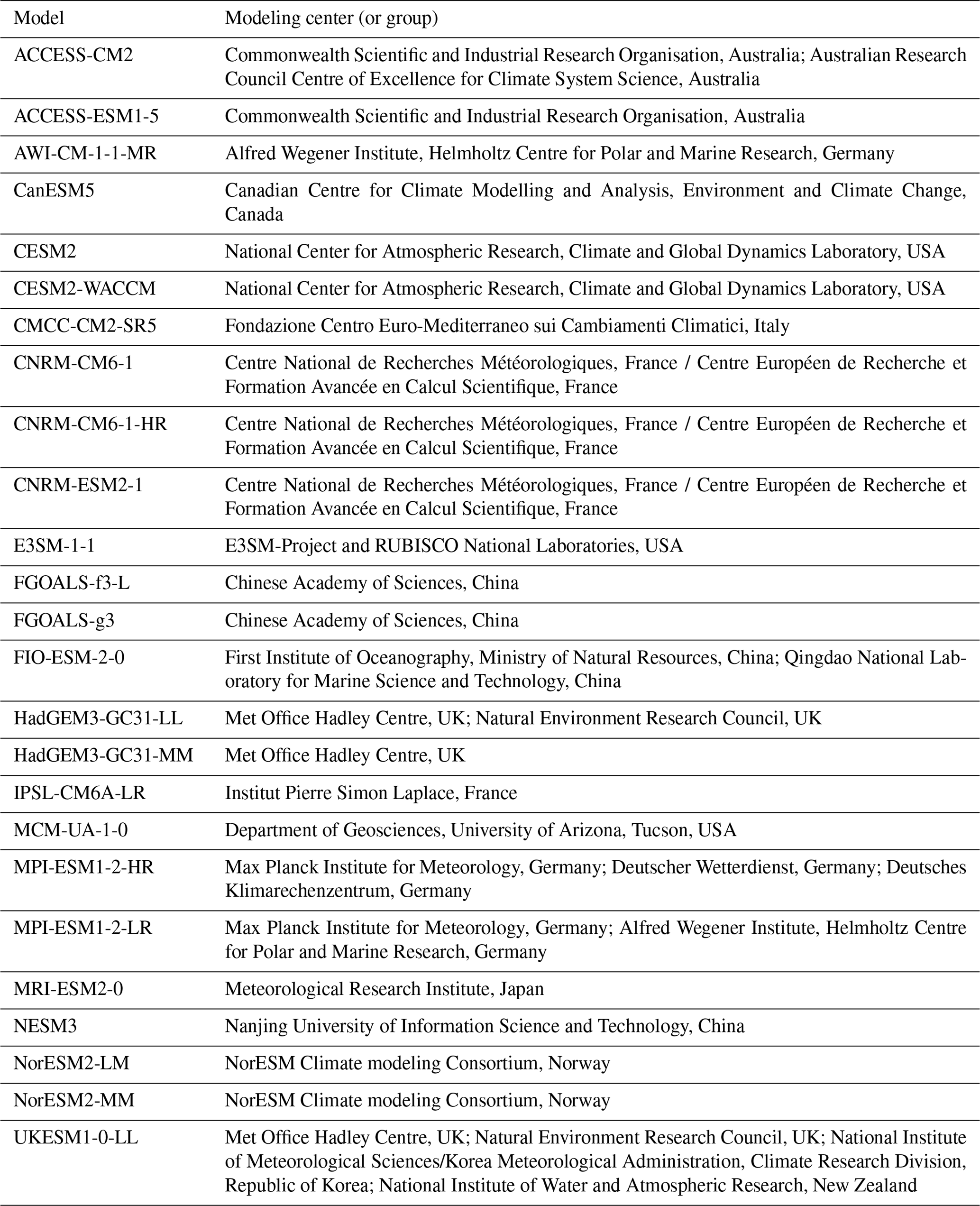
Table A1 List of the 25 employed CMIP6 models and the modeling groups providing them.