the Creative Commons Attribution 4.0 License.
the Creative Commons Attribution 4.0 License.
 | 09 Mar 2022
Global evaluation of the Ecosystem Demography model (ED v3.0)
Lei Ma
George Hurtt
Lesley Ott
Ritvik Sahajpal
Justin Fisk
Rachel Lamb
Steve Flanagan
Louise Chini
Abhishek Chatterjee
Joseph Sullivan
Terrestrial ecosystems play a critical role in the global carbon cycle but have highly uncertain future dynamics. Ecosystem modeling that includes the scaling up of underlying mechanistic ecological processes has the potential to improve the accuracy of future projections while retaining key process-level detail. Over the past two decades, multiple modeling advances have been made to meet this challenge, such as the Ecosystem Demography (ED) model and its derivatives, including ED2 and FATES. Here, we present the global evaluation of the Ecosystem Demography model (ED v3.0), which, like its predecessors, features the formal scaling of physiological processes for individual-based vegetation dynamics to ecosystem scales, together with integrated submodules of soil biogeochemistry and soil hydrology, while retaining explicit tracking of vegetation 3-D structure. This new model version builds on previous versions and provides the first global calibration and evaluation, global tracking of the effects of climate and land-use change on vegetation 3-D structure, spin-up process and input datasets, as well as numerous other advances. Model evaluation was performed with respect to a set of important benchmarking datasets, and model estimates were within observational constraints for multiple key variables, including (i) global patterns of dominant plant functional types (broadleaf vs. evergreen), (ii) the spatial distribution, seasonal cycle, and interannual trends for global gross primary production (GPP), (iii) the global interannual variability of net biome production (NBP) and (iv) global patterns of vertical structure, including leaf area and canopy height. With this global model version, it is now possible to simulate vegetation dynamics from local to global scales and from seconds to centuries with a consistent mechanistic modeling framework amendable to data from multiple traditional and new remote sensing sources, including lidar.
- Article
(9989 KB) - Full-text XML
-
Supplement
(473 KB) - BibTeX
- EndNote


Terrestrial ecosystems and the associated carbon cycle are of critical importance in providing ecosystem services and regulating global climate. Plants store approximately 450–650 Pg C as biomass globally. They remove approximately 120 Pg C from the atmosphere each year through photosynthesis, and release a similar magnitude of carbon into the atmosphere through respiration (Beer et al., 2010; Ciais et al., 2014b). Human activities in past centuries have significantly impacted terrestrial ecosystems through biophysical and biogeochemical mechanisms (Cramer et al., 2001; Walther et al., 2002; Brovkin et al., 2004; Pielke et al., 2011). Quantification, attribution and future projections of the terrestrial carbon sink require an in-depth understanding of the underlying ecological processes and their sophisticated responses and feedbacks to climate change, elevated CO2, and land-use and land-cover change (LULCC) across multiple biomes and spatial and temporal scales (Canadell et al., 2007; Erb et al., 2013; Keenan and Williams, 2018). This demand for information has driven the emergence and development of dynamic global ecosystem models (DGVMs), which simplify the structure and functioning of global vegetation into several plant functional types and simulate vegetation distribution and associated biogeochemical and hydrological cycles with ecophysiological principles (Prentice et al., 2007; Prentice and Cowling, 2013). The first generation of DGVMs have been successfully used to address a variety of carbon-cycle-related questions and integrated into Earth system models (ESMs) (Cramer et al., 2001; Sitch et al., 2008). Subsequent developments have improved the representation of vegetation demographic processes within ESMs, and include the Ecosystem Demography model (ED) (Hurtt et al., 1998; Moorcroft et al., 2001), ED2 (Medvigy, 2006; Medvigy et al., 2009; Longo et al., 2019), CLM(ED) (Fisher et al., 2015; Lawrence et al., 2019; Massoud et al., 2019), SEIB-DGVM (Spatially-Explicit Individual-based Dynamic Global Vegetation Model) (Sato et al., 2007), LPJ-GUESS (Lund-Potsdam-Jena General Ecosystem Simulator) (Smith et al., 2001, 2014) and GFDL-LM3-PPA (Geophysical Fluid Dynamics Laboratory Land Model 3 with the Perfect Plasticity Approximation) (Weng et al., 2015, as summarized in Fisher et al., 2018).
In addition to model development, model evaluation is important for assessing model uncertainties and identifying processes that need particular improvements (Anav et al., 2013; Luo et al., 2012; Eyring et al., 2019). Considerable effort has been spent on standardizing evaluation practices and developing a comprehensive benchmarking system (Abramowitz, 2012; Collier et al., 2018; Eyring et al., 2016; Randerson et al., 2009). For example, a benchmarking system from the International Land Model Benchmarking (ILAMB) project has been increasingly used to evaluate ecosystem and climate models (Collier et al., 2018; Ghimire et al., 2016; Luo et al., 2012). In parallel, new observations are providing new opportunities to initialize and test models. Of particular relevance for ecosystem models is the advent of spaceborne lidar missions (i.e., GEDI and ICESat-2) (Dubayah et al., 2020a; Markus et al., 2017), which provide unprecedented global observations of forest structure, including the vertical distribution of leaf foliage. Building on that past work, and utilizing new observations, an updated and systematic evaluation of model performance across multiple variables is now possible.
Here, we present the global evaluation of Ecosystem Demography v3.0. The ED model was developed two decades ago using a formal scaling approach (size- and age-structured approximation, SAS) to efficiently approximate the expected dynamics of individual-based forest dynamics (Hurtt et al., 1998; Moorcroft et al., 2001). Since its emergence, the ED model has been continuously developed and applied to various regions and spatial scales with land-use changes and lidar observations (Hurtt et al., 2002, 2004). In the original paper, the model was implemented at the site scale and primarily evaluated for aboveground biomass accumulation during succession using chronosequence field data, and at the regional scale using 1∘-resolution data on potential biomass, soil carbon, and net primary productivity (NPP) (Moorcroft et al., 2001). Most recently, ED was implemented at a high spatial resolution (90 m) over a regional domain of the Northeastern United States and evaluated for aboveground biomass using wall-to-wall lidar-based estimates of contemporary biomass at that spatial resolution (Hurtt et al., 2019b; Ma et al., 2021b). The evaluation included >30 million grid cell pairs and >103 forest inventory field plots. This progression of development includes a range of model capabilities, spatial resolutions and evaluation data, spanning from coarse-resolution potential vegetation to high-spatial-resolution contemporary conditions at regional scales. However, the development and evaluation of ED at the global scale for contemporary conditions has not yet been accomplished. In this study, ED v3.0 is evaluated at global scales for the first time. Multiple key variables are considered in the evaluation, including benchmark datasets on vegetation distribution, vegetation structure, and carbon and water fluxes.
ED v3.0 is built upon a series of previous model developments (Moorcroft et al., 2001; Hurtt et al., 2002; Albani et al., 2006; Fisk, 2015; Flanagan et al., 2019). To extend ED's capabilities globally, several additional modifications were introduced to capture the global vegetation distribution across biomes and related carbon stocks and fluxes. Below, a summary of the ED approach and recent modifications is provided. The full descriptions of each submodule can be found in the Supplement, along with tables of parameter values. To conduct the model evaluation, a model experimental protocol including equilibrium and transient simulations was developed, and relevant forcing data were identified from global existing datasets. Model simulations were then compared to benchmarking datasets.

Figure 1Diagram of the vegetation representation scheme in the ED model. Globe consists of land grids with a fixed spatial resolution. A grid consists of patches with different ages from last disturbance and land-use types, and patch areas dynamically change over time as a result of disturbance and land-use changes. A patch consists of different plant functional types and sizes. Plants in a cohort are depicted by properties including individual density, canopy height, diameter at breast (DBH), and biomass in leaf, sapwood, structural tissue and fine roots, and all these properties are simulated as a result of interactions with the environment and other cohorts. Note that not all properties are shown here.
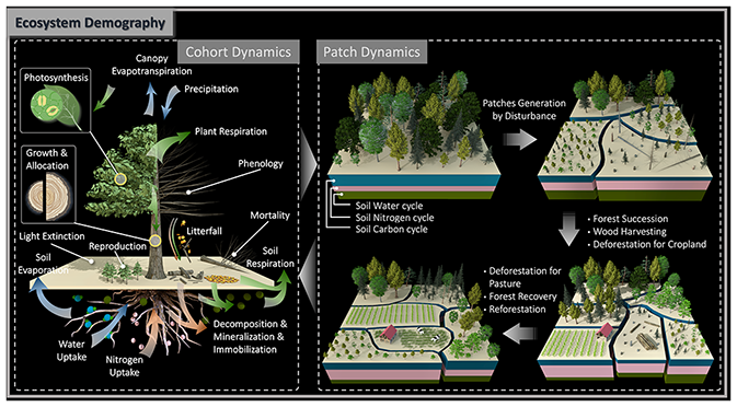
Figure 2Schematic diagram of processes represented in the ED model. Dynamics at cohort level consist of carbon-related flow (green arrows), water-related flow (blue arrows) and nitrogen-related flow (orange arrows). Carbon dynamics include carbon assimilation by photosynthesis, carbon allocation for plant growth in height/DBH, reproduction and respiration, carbon translocation between plants and soil through tissue turnover as litterfall and dead plants due to mortality, and carbon decomposition and respiration in soil carbon pools. Water dynamics include water inputs from precipitation and infiltration into soil, uptake by vegetation, and evaporation and transpiration from the soil and canopy. Nitrogen dynamics include nitrogen uptake from soil pools, translocation from vegetation to soil through litterfall and dead plants, and mineralization and immobilization in soil. Note that not all processes that ED characterizes are depicted here. Dynamics at the patch level consist of consequences of a variety of disturbance events, both natural and anthropogenic. Patch dynamics include disturbance-driven patch heterogenization in age and areas, forest succession, wood harvesting, deforestation for cropland and pasture expansion, and forest recovery and reforestation from abandoned cropland, harvested forest and pasture.
2.1 Model
The ED model is an individual-based prognostic ecosystem model (Moorcroft et al., 2001). By integrating submodules of growth, mortality, hydrology, carbon cycle and soil biogeochemistry, ED can track plant dynamics, including growth, mortality and reproduction. Along with plant dynamics, ED can track the carbon cycle, including carbon uptake by leaf photosynthesis, carbon allocation to biomass growth in leaves, roots and stems, carbon redistribution from plants to soil based on plant tissue turnover from dead plants due to mortality and disturbance, carbon decomposition in various pools (metabolic litter pool, structural litter pool, soil slow pool, soil passive pool, wood product pool, harvested crop pool, etc.), as well as carbon combustion from fire (Figs. 1 and 2). Over the last two decades, ED has been continuously developed and combined with lidar and land-use change data to predict ecosystem dynamics and associated water and carbon fluxes across spatial scales (e.g., site to regional and continental) and temporal scales (e.g., short-term seasonal to long-term decadal and century) (Hurtt et al., 2002, 2004, 2010, 2016; Fisk et al., 2013; Flanagan et al., 2019). ED distinguishes itself from most other ecosystem models by explicitly tracking vegetation structure and scaling fine-scale physiological processes to large scale ecosystem dynamics (Hurtt et al., 1998; Moorcroft et al., 2001; Fisher et al., 2018). In ED, vegetation structure (e.g., height and diameter at breast height) and physiological processes (e.g., leaf photosynthesis and phenology) are modeled at the individual scale, where individual plants compete mechanically for light, water and nutrients. During implementation, this horizontal heterogeneity is tracked through cohort and patch demography. Explicitly modeling vegetation height facilitates a potential connection to lidar data.
Additional modifications
Major modifications in ED v3.0 focus on four areas: plant functional type representation, leaf level physiology, hydrology and wood products. These areas have been identified as particularly important for improving model performance globally.
Plant functional types (PFTs) describe the characteristics of vegetation in different representative groups for modeling. In previous ED versions, various PFT combinations were implemented to represent vegetation in the respective regions where the model was implemented. In the original implementation of ED for Central and South America, four PFTs were represented (i.e., early-successional broadleaf, middle-successional broadleaf, late-successional broadleaf and C4 grasses; Moorcroft et al., 2001). In a subsequent implementation over North America, two additional PFTs (i.e., northern pines and southern pines) were proposed in Albani et al. (2006). Here, these PFTs are included and further refined as seven major PFTs: early-successional broadleaf trees (EaSBT), middle-successional broadleaf trees (MiSBT), late-successional broadleaf trees (LaSBT), northern and southern pines (NSP), late-successional conifers (LaSC), C3 shrubs and grasses (C3ShG), and C4 shrubs and grasses (C4ShG) (Sect. S1 in the Supplement). Tropical and non-tropical subtypes of the broadleaf PFTs (i.e., EaSBT, MiSBT, and LaSBT) are distinguished. These PFTs primarily differ in phenology, leaf physiological traits, allometry, mortality rate and dispersal distance. As in previous versions of ED, the spatial distribution of PFTs is mechanistically determined by individual competition for light, water and nutrients. No quasi-equilibrium climate–vegetation relationships, or other assumptions or observations, are used to constrain the presence or absence of PFTs.
Leaf physiology determines short-term (i.e., < hourly) leaf-level carbon and water exchanges in response to environmental conditions (air temperature, shortwave radiation, air humidity, wind speed and CO2 level). The representation of leaf-level physiology in previous versions of ED (Moorcroft et al., 2001) was taken from IBIS (Foley et al., 1996), which in turn was based on prior work from Farquhar, Collatz, Ball, Berry and others (Farquhar and Sharkey, 1982; Ball et al., 1987; Collatz et al., 1991, 1992). Here, ED's representation of leaf-level physiology is reformulated for C3 and C4 pathways (Farquhar et al., 1980; von Caemmerer and Furbank, 1999) with added boundary layer conductance for diffusing water vapor and CO2 between the ambient air and leaf surface, and parameterized with temperature dependence functions from other studies (Bernacchi et al., 2001; von Caemmerer et al., 2009; Kattge and Knorr, 2007; Massad et al., 2007; von Caemmerer, 2000, Sect. S3).
Hydrology controls the water available for vegetation. The hydrology submodule in ED tracks soil moisture dynamics between incoming water flow from precipitation and outgoing flow through percolation, runoff and transpiration. Previous ED versions did not include evaporation from the soil and canopy and also did not account for snow dynamics. Here, evaporation from the soil and canopy is estimated based on the Penman–Monteith (P-M) equation (Monteith, 1965; Mu et al., 2011). In addition, a simple snow dynamics process is introduced to decrease water availability for plants when the air temperature drops below freezing point or to increase it when the air temperature rises above freezing point at a rate that depends on the air temperature. More details can be found in Sect. S9.
Land-use activities (e.g., deforestation and wood harvesting) remove vegetation carbon from ecosystems for various purposes. This carbon is traditionally tracked in wood product pools with different lifetimes and temporal emissions to the atmosphere. The previous land-use submodule in ED only tracked changes in vegetation and soil carbon during various land-use activities; it did not track subsequent decay processes of product pools (Hurtt et al., 2002). In ED v3.0, three wood product pools are added to track the life cycles of harvested wood and associated decay processes (Sect. S11). Wood product pools gain carbon from land-use activities such as wood harvesting or deforestation and lose carbon through decay and emissions to the atmosphere. The loadings of these product pools, and their decay rates, are based on a prior study (Hansis et al., 2015).
2.2 Model initialization and overview of experiments
The global spin-up of ED initialized ecosystems to contemporary conditions by taking into account climate change, rising CO2 and land-use change. This global spin-up comprised two separate runs at 0.5∘ spatial resolution. The first run, called the “equilibrium simulation,” ran ED from the initial conditions to equilibrium. This run was performed for 1000 years, by which time the PFT composition and carbon pools of vegetation and soil had reached dynamic equilibrium. The second run, called “transient simulation,” restarted from the end of the equilibrium simulation and simulated for 1166 years, corresponding to the period AD 851–AD 2016, with varying CO2 levels, land-use change and climate variability. Both runs were driven with meteorological forcing from NASA's Modern-Era Retrospective analysis for Research and Applications, version 2 (MERRA2) (Gelaro et al., 2017) and surface CO2 concentrations from the NOAA CarbonTracker Database, version 2016 (NOAA CT2016) (Peters et al., 2007, with updates documented at http://carbontracker.noaa.gov, last access: 1 March 2022). Additionally, the transient simulation ran the utilized prescribed burned area from the Global Fire Emissions Database, version 4 (GFED4) (Randerson et al., 2015) and forced land-use change from Land Use Harmonization, version 2 (LUH2) (Hurtt et al., 2019a, 2020). Details of these simulations are provided below.
The equilibrium simulation was started from bare ground, where the soil and vegetation carbon pools were set at zero, and all PFTs were initialized with equal seedling density for all patches and all grid cells over the globe. This run was driven for 1000 years with MERRA2 climatology for 1981–1990 and NOAA CT2016 average surface CO2 between 2001 and 2014 (with spatial variation and the global average rescaled to 280 ppm). No climatic envelope or potential biome maps were used to constrain the PFT spatial distribution; competition determined the final PFT distributions, vegetation structure and carbon stocks. The land-use change module was disabled in this run of the simulation.
The transient simulation was restarted from equilibrium conditions. The land-use change submodule was activated and all land-use transition types from LUH2 were incorporated into the simulation at annual time steps. These transitions included changes in agriculture and forest extent, shifting cultivation and wood harvesting, among others. MERRA2, NOAA CT2016 and GFED were used throughout the simulation with varying temporal settings depending on data availability. Specifically, for MERRA2, the climatology between 1981 and 1990 was used until 1981, and annual meteorology was used subsequently. For NOAA CT2016, the average surface CO2 concentration between 2001 and 2014, which varies spatially and grows over time, was used until 2000, while annual NOAA CT2016 surface CO2 concentrations were used subsequently. For the GFED4 burned area, the average between 1996 and 2016 was used until 1996, after which the annual burned area was used.
2.3 Forcing data
Meteorological variables utilized from MERRA2 include surface air temperature (TLML), surface specific humidity (QLML), precipitation (PRECTOTCORR), incident shortwave radiation (SWGDN), surface wind speed (SPEED) and multilayer soil temperature (TSOIL1–TSOIL3). Original estimates of surface air temperature, surface specific humidity, incident shortwave radiation and surface wind speed were averaged from daily hourly to monthly hourly for each year between 1981 to 2016. The resulting annual monthly averages of diurnal meteorological variables were used to drive the leaf physiology submodule in ED. Hourly surface air temperature, precipitation and soil temperature were also aggregated to monthly averages for each year between 1981 to 2016 and then used to drive the soil hydrology, phenology, evapotranspiration and biogeochemical modules in ED.
Surface CO2 concentration was extracted from the lowest vertical level of NOAA CT2016 CO2 mole fraction that varies temporally and spatially. The original datasets were first linearly interpolated from 3∘ × 2∘ (longitude × latitude) to 0.5∘ × 0.5∘ and from 3 h to hourly, and then averaged to give monthly hourly estimates for each grid cell and each year between 2001 and 2014, resulting in surface CO2 concentration maps with 4032 timesteps (14 years, 24 h, 12 months) for each 0.5∘ × 0.5∘ grid. The surface CO2 concentration maps were used to drive the transient simulation from 850 to 2000, retaining the average spatial variation between 2001 and 2014 and applying a scaling factor to force the global annual average CO2 concentration to remain at 280 ppm before 1850 and then grow linearly to 310 ppm in 1950 and 375 ppm in 2000. This increasing trend in the global average matches observed CO2 growth rates from Keeling (2008).
LUC forcing was derived from LUH2 (version v2h) for years 850–2015 (Hurtt et al., 2019a, 2020). The original land-use state and land-use transitions were aggregated from a spatial resolution of 0.25∘ × 0.25∘ to 0.5∘ × 0.5∘ for each year between 850 and 2015. Subtypes of land-use states and associated transitions were grouped into the major land-use types of the model's predecessor version (LUH1). Specifically, the sub-crop types of C3 annual crops (c3ann), C3 perennial crops (c3per), C4 annual crops (c4ann), C4 perennial crops (c4per) and C3 nitrogen-fixing crops (c3nfx) were all merged as cropland. Forested primary land (primf) and non-forested primary land (primn) were merged as primary land; forested secondary land (secdf) and non-forested secondary land were merged as secondary land, and managed pasture (pastr) and rangeland were merged as pasture. Note that all types of land-use transitions and gross transition rates were used in ED's land-use module.
Soil properties, including depth, hydraulic conductivity, and residual and saturated volumetric water content, are important for determining plant water availability. These soil properties were taken from Montzka et al. (2017). Additional details can be found in the Supplement (Sect. S9, hydrology submodule).
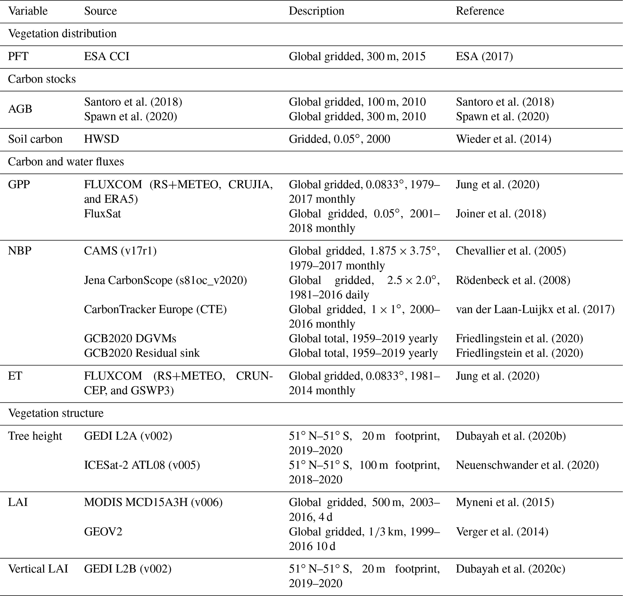
Table 1Summary of benchmarking datasets used for ED model evaluation.
2.4 Model evaluation
A benchmarking package of data (Table 1) was collected to evaluate ED performance. Eight critical variables, proven to be important for terrestrial biogeochemical cycles (Spafford and MacDougall, 2021), were assessed in four categories: PFT distribution, carbon stocks in vegetation and soil, carbon and water fluxes, and vegetation structures in terms of canopy height and vertical leaf area index (LAI). The evaluation was carried out at different spatial (grid, latitudinal and biome) and temporal (climatological, seasonal and interannual) scales. For each variable, a widely used dataset was used for reference. In some cases, these spanned different years. An important feature of our method was the adjustment of the simulation years from ED to match each benchmarking dataset.
2.4.1 Vegetation distribution
The satellite-based land-cover product ESA CCI was used to examine the distribution of three modeled PFTs: grass, broadleaf trees and needleleaf trees (ESA, 2017). Many satellite-based land-cover datasets differ largely from ED in PFT definition. For example, no successional PFTs exist in ESA CCI land-cover types. Thus, the native PFTs in ED and ESA CCI both have to be aggregated to broader categories such as broadleaf PFTs, needleleaf PFTs and grass PFTs. To do this, the 22 native land-cover classes of ESA CCI were first reclassified to “broadleaf evergreen tree,” “broadleaf deciduous tree,” “needleleaf evergreen tree,” “needleleaf deciduous tree,” “natural grass” and “manned grass” using a cross-walk table (Poulter et al., 2015). They were then further merged by phenology type and aggregated to 0.5∘, resulting in PFT fraction maps of broadleaf PFTs, needleleaf PFTs, and grass and shrub PFTs. ED PFTs of EaSBT, MiSBT and LaSBT were merged as broadleaf PFTs, NSP and LaSC were merged as needleleaf PFTs, and C3ShG and C4ShG were merged as grass and shrub PFTs.
2.4.2 Carbon fluxes
Evaluation of carbon fluxes focused on gross primary production (GPP) and net biome production (NBP). Modeled GPP was evaluated with respect to spatial pattern, seasonality and interannual variability using two satellite-data-driven GPP datasets, FLUXCOM (Jung et al., 2020) and FluxSat (Joiner et al., 2018), and the satellite-retrieved sun-induced chlorophyll fluorescence (CSIF) dataset (Zhang et al., 2018). The FLUXCOM and FluxSat datasets are derived from a data-driven approach that combines carbon flux measurements from FLUXNET and satellite observations from MODIS. Major differences between FLUXCOM and FluxSat include the use of meteorological forcing and the specific approach used. FLUXCOM used meteorological forcing and a machine learning approach, while FluxSat used a simplified light-use efficiency model that does not rely upon meteorological forcing. FluxSat also used satellite-based sun-induced chlorophyll fluorescence (SIF) to delineate highly productive regions. Satellite measurements of SIF have recently been suggested as a promising proxy for terrestrial GPP, as they exhibit high sensitivity to plant photosynthetic activities (Lee et al., 2013; Guanter et al., 2014; Yang et al., 2015). In this study, we chose the CSIF dataset for its improved spatiotemporal continuity. CSIF is generated by fusing Orbiting Carbon Observatory-2 (OCO-2)-retrieved SIF and MODIS reflectance data using a machine learning approach. FLUXCOM, FluxSat and CSIF were all resampled to give monthly estimates at 0.5∘ × 0.5∘ spatial resolution before the evaluation.

Figure 3Spatial distribution of broadleaf PFTs, needleleaf PFTs, and grass and shrub PFTs in 2015 from ED (a, c, e), and from ESA CCI (b, d, f). The corresponding latitudinal total areas are compared in (g) and (h).
Modeled NBP was compared against multiple sources, including estimates from process-based models, atmospheric inversions and the 2020 global carbon budget (GCB2020) (Friedlingstein et al., 2020). For process-based models, 17 DGVMs reported in the GCB2020 were used to calculate the respective net land sink by differencing land-uptake and land-use emissions estimates (i.e., SLAND−ELUC). For atmospheric inversions, three systems are used, namely CarbonTracker Europe (CTE) (van der Laan-Luijkx et al., 2017), Jena CarboScope (version s81oc) (Rödenbeck et al., 2008) and the Copernicus Atmosphere Monitoring Service (CAMS) (Chevallier et al., 2005). The three inversions all derive surface carbon fluxes using atmospheric CO2 measurements, prior constraints on fluxes, and an uncertainty and atmospheric transport model, but vary with respect to the specific data, prior constraints and transport models used (Peylin et al., 2013). In the GCB2020, the residual terrestrial sink was used, which was calculated as the total emissions from fossil fuel and land-use change minus the atmospheric CO2 growth rate and ocean sink (i.e., ).
2.4.3 Carbon stocks
Modeled carbon pools were evaluated with regards to vegetation aboveground biomass (AGB) and soil carbon. The reference AGB data included estimates from Santoro et al. (2018) and Spawn et al. (2020). These two AGB datasets provide high spatial resolution (e.g., 100–1000 m) wall-to-wall global estimates of the year 2010, but differ in their methodologies. Specifically, AGB from Santoro et al. (2018) was produced by combining spaceborne synthetic aperture radar (SAR) (ALOS PLASAR, Envisat ASAR), Landsat-7, and lidar (from the Ice, Cloud, and land Elevation Satellite: ICESat) observations. AGB from Spawn et al. (2020) includes biomass of forests and other woody non-forest plants. Reference soil carbon was from the Harmonized World Soil Database (HWSD) (Wieder et al., 2014), and included soil carbon for topsoil (0–30 cm) and subsoil (30–100 cm).
2.4.4 Water fluxes
Modeled ET was evaluated against the FLUXCOM dataset (Jung et al., 2020), which used meteorological forcing, remote sensing data and a machine learning approach to scale up the measurements from FLUXNET eddy covariance towers to the global scale. This dataset provides gridded estimates at a resolution of 0.0833∘ for the period 1981–2014. The FLUXCOM dataset was resampled to monthly estimates at 0.5∘ × 0.5∘ spatial resolution before evaluation.
2.4.5 Vegetation structure
Evaluation of modeled forest structure focused on the total and vertical distributions of LAI and tree canopy height. Two reference LAI products, namely MODIS MCD15A3H (Myneni et al., 2015) and GEOV2 LAI (Verger et al., 2014), were used for evaluating total LAI in terms of spatial distribution, seasonality and interannual variability. The MODIS and GEOV2 LAI datasets were both derived from passive optical observations with empirically based inversion methods that relate leaf area with optical canopy reflectance or vegetation indices; however, these two products vary by the source of optical observations and the inversion method chosen. The reference vertical LAI was from the Global Ecosystem Dynamics Investigation (GEDI) L2B products, which retrieves the leaf vertical distribution from lidar waveform return (Dubayah et al., 2020c). Reference canopy height data were based on direct forest structure observations from GEDI L2A (Dubayah et al., 2020b) and the ICESat-2 ATL08 products (Neuenschwander et al., 2020). Mean canopy height was generated at 0.5∘ spatial resolution from the relative height 98th percentile (RH98) of all GEDI L2A footprints and the canopy top height (h_canopy) of all ICESat-2 ATL08 segments of good quality.
ED results were evaluated across four primary categories: PFT distribution, vegetation and soil carbon pools, carbon and water fluxes, and vegetation structure. Evaluation included comparing modeled global quantities and their associated spatial and temporal patterns to the benchmarking datasets.

Figure 4AGB in 2010 from ED (a), Spawn et al. (2020) (b) and Santoro et al. (2018) (c), with the latitudinal average AGBs compared in (d).
3.1 Evaluation of the PFT distribution
Global total areas of broadleaf PFTs, needleleaf PFTs, and grass and shrub PFTs were estimated by ED to be 24.30, 8.93 and 24.63 million km2, respectively. These results were compared to the respective estimated global PFT areas from ESA CCI data: 20.13, 10.65 and 41.49 million km2. The global spatial distributions and corresponding zonal distributions of broadleaf PFTs, needleleaf PFTs, and grass and shrub PFTs are shown in Fig. 3. In this comparison, the major patterns of the ED estimated PFT distribution were similar to the observed distribution of PFTs. ED estimated needleleaf PFTs were dominant at high latitudes, broadleaf PFTs dominated in the tropics, and grass and shrub PFTs were widespread globally. ED also predicted the observed coexistence of broadleaf and needleleaf PFTs in southern China and the eastern US. However, beyond these major patterns, ED estimates differed in some specific regions. For example, ED predicted the existence of needleleaf PFTs along the Andes Mountains in South America and in southern Australia. While this pattern was not evident in the ESA CCI data, there are other studies based on ground observations that support it (Farjon and Filer, 2013). ED also estimated more broadleaf PFTs in eastern Europe and southern China, less broadleaf PFTs in Africa savanna, less needleleaf PFTs in east Siberia, and less grass and shrub PFTs in both the African savanna and northern China. Analogous results can also be seen zonally, where major patterns of PFTs are broadly similar to those observed but with some specific differences. In terms of zonal distribution per PFT, the smallest discrepancies between ED and ESA CCI appear for broadleaf PFTs, followed by needleleaf PFTs and grass and shrub PFTs. Spatial distribution maps for each of the seven PFTs from ED can be found in Fig. S1.
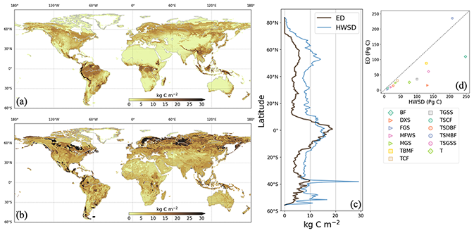
Figure 5Soil carbon density in 2000 from ED (a) and HWSD (b). Latitudinal average density and total stocks per biome are compared in (c) and (d), respectively. In the legend of (d), BF is boreal forests/taiga, DXS is deserts and xeric shrublands, FGS is flooded grasslands and savannas, MFWS is Mediterranean forests, woodlands, and scrub, MGS is montane grasslands and shrublands, TBMF is temperate broadleaf and mixed forests, TCF is temperate coniferous forests, TGSS is temperate grasslands, savannas, and shrublands, TSCF is tropical and subtropical coniferous forests, TSDBF is tropical and subtropical dry broadleaf forests, TSMBF is tropical and subtropical moist broadleaf forests, TSGSS is tropical and subtropical grasslands, savannas, and shrublands, and T is tundra.
3.2 Evaluation of AGB and soil carbon
ED estimates of AGB were compared to corresponding benchmark data. ED estimated the global total aboveground vegetation carbon (including forest and non-forest) at 298 Pg C in 2010. This compares to 283 and 297 Pg C, as estimated by Spawn et al. (2020) and Santoro et al. (2018). ED's estimate of the spatial pattern of AGB was also comparable to those of both benchmark datasets, with the highest biomass densities found across the tropics (i.e., the Amazon rainforest, the Congo river basin and southeast Asia) and declining biomass densities northward towards the temperate and boreal regions. For example, similar to observations, the average estimated AGB density was ∼15 kg C m−2 in the tropics and less than 2.5 kg C m−2 across temperate and boreal regions (Fig. 4d). In addition, the AGB transition along the African forest–savanna zone was represented by ED, albeit with lower values in the savanna. Major discrepancies between ED and benchmarking data appear in southern China, southeast Asia and southeast Brazil.
ED estimates of soil carbon were compared to benchmark data on soil carbon. ED estimated the total global soil carbon at 671 Pg C in 2000, which was within the range of CMIP5 ESMs (510–3040 Pg C) (Todd-Brown et al., 2013) but lower than the HWSD estimate of 1201 Pg C. Comparing total stocks at the biome level (Fig. 5d) showed that ED generally reproduced soil carbon variation across biomes but notably underestimated carbon in boreal forest/taiga, deserts and xeric shrublands, tropical and subtropical grasslands, savannas and shrubland. The soil carbon map from ED revealed different spatial patterns compared to HWSD, with less spatial heterogeneity and fewer regions with densities above 30 kg C m−2.

Figure 6Average annual GPP between 2001 and 2016 from ED (a), FLUXCOM (b), FluxSat (c) and the CSIF (d). A comparison of the latitudinal average GPP values is shown in (e).
3.3 Evaluation of GPP, NBP and ET
Globally, the ED estimate of average annual GPP was 134 Pg C yr−1 between 2001–2016, which compares to 120 Pg C yr−1 from FLUXCOM and 136 Pg C yr−1 from FluxSat over the same period. The spatial pattern of GPP from ED was also compared to benchmark values at the grid and latitudinal scales (Fig. 6). Similar to observations, the areas of highest productivity occur in the tropics, followed by the temperate and boreal regions. For the tropics, ED was ∼0.5 kg C m−2 yr−1 higher than FLUXCOM and ∼ 0.2 kg C m−2 higher than FluxSat, but lower than both over the African savanna. Additionally, ED was higher in southern China and Brazil than in either benchmark dataset. A notably increasing annual trend was seen in the total global GPP in both ED and FluxSat estimates between 2001 and 2016 as well as in the globally averaged CSIF (Fig. 7). ED also reproduced the GPP interannual variability from FluxSat, FLUXCOM and CSIF, dipping in the years 2005, 2012 and 2015 and peaking in 2006, 2011 and 2014. Regarding latitudinal seasonality at the biome scale (Fig. 8), ED captured the GPP timing for most latitudinal zones, including 60–90∘ N, 45–60∘ N, 15–30∘ N and 60–30∘ S. Major differences appeared at 30–45∘ N, where ED showed a decrease from July–September, and at 15∘ S–0∘, where ED showed delayed monthly timing of the lowest annual GPP values.

Figure 7Time series of the global annual total GPP (from ED, FLUXCOM and FluxSat) and the global annual average CSIF. Their interannual anomalies are shown in the inset.
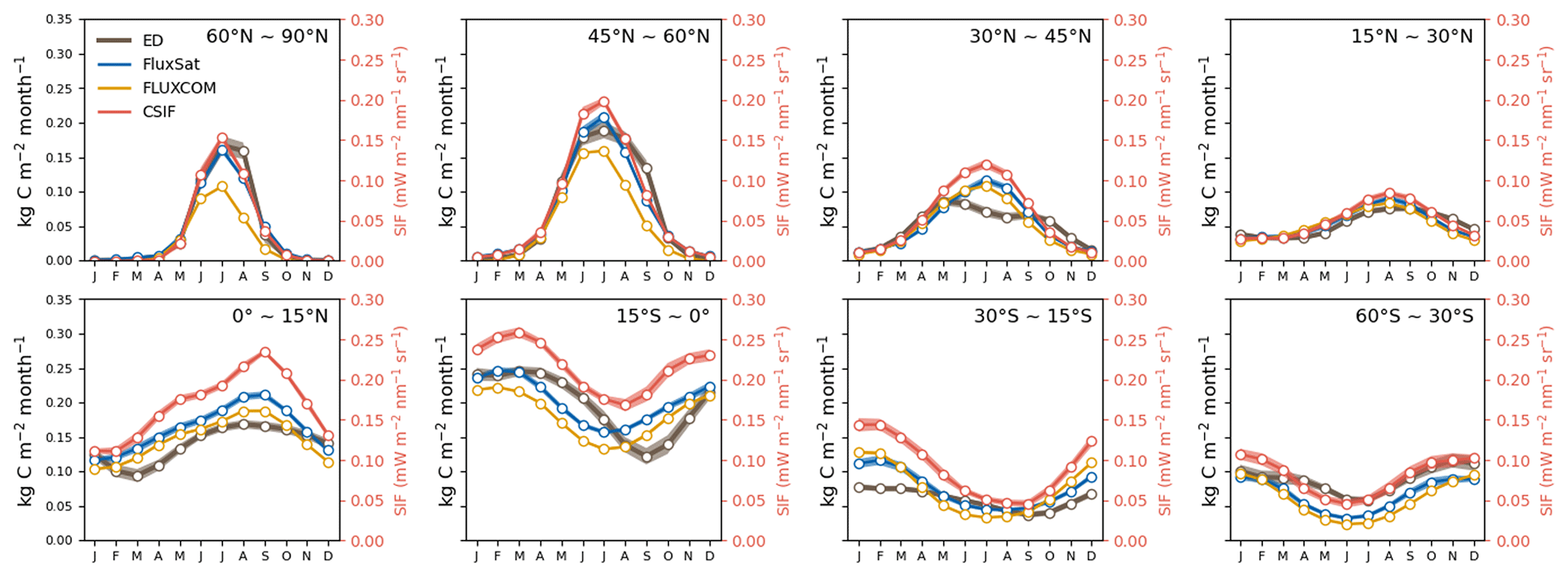
Figure 8Average seasonal cycle (2001–2016) of GPP (from ED, FLUXCOM and FluxSat) and CSIF by latitudinal band.
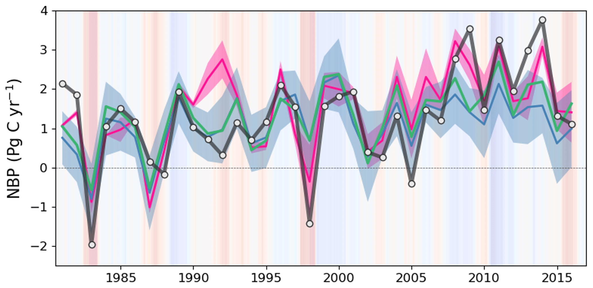
Figure 9Global annual NBP between 1981 and 2016 from ED (black line), DGVMs from the GCB2020 (ensemble average shown as a blue line, with the ±1σ spread shown as blue shading), the ensemble of atmospheric inversions (ensemble average shown as a pink line, with the ±1σ spread shown as pink shading) and the terrestrial residual sink of the GCB2020 (green line). Positive values indicate net carbon uptake from land. Background shading represents the bimonthly Multivariate El Niño/Southern Oscillation (ENSO) index, where red indicates El Niño and blue indicates La Niña.
Globally, the ED estimate of average annual NBP between 1981 and 2016 was 1.99 Pg C yr−1, which can be compared to 1.21–1.80 Pg C yr−1 from atmospheric inversions, 1.11 Pg C yr−1 from DGVMs, and 1.31 Pg C yr−1 from the GCB2020 residual terrestrial sink. ED estimates were also compared to benchmark datasets on global changes over time (Fig. 9). Similar to the references, ED estimated an increasing trend with substantial interannual variation during the 1981–2015 period. This variation included reductions in El Niño years (such as 1983, 1998 and 2015) and increases in La Niña years (such as 1989, 2001–2002 and 2011). An exception is 1991–1992, where ED and DGVMs were both lower than atmospheric inversions. This period includes the Mt. Pinatubo eruption, the effect of which is not included in the shortwave radiation forcing of GCB2020 DGVMs or ED (Mercado et al., 2009; Friedlingstein et al., 2020). During the period 2007–2016, ED produced a continued increasing trend, as reflected in the mean of atmospheric inversions but not the mean of DGVMs. Specifically, ED estimated NBP averaged 2.34 Pg C yr−1 from 2007 to 2016, which was within the range of the atmospheric inversion estimates (1.77–2.64 Pg C yr−1) and DGVM estimates (0.58–2.82 Pg C yr−1), but higher than either the mean of DGVMs (1.40 Pg C yr−1) or the GCB2020 residual terrestrial sink (1.81 Pg C yr−1). Despite the similarities in global trends, the latitudinal comparison between ED and atmospheric inversions indicated contrasting attribution of the global sink (Fig. 10). In comparison to the atmospheric inversions, ED predicted a stronger sink in the tropics and a weaker sink in the Northern Hemisphere. Such a pattern was highlighted in the global carbon budget (Friedlingstein et al., 2020), where process-based models and the atmospheric inversions generally show less agreement on the spatial pattern of the carbon sink in these two regions. There is recognized uncertainty about the underlying actual pattern due in part to the in situ network, which is spatially biased towards the mid-latitudes (i.e., more observational sites) relative to the tropics (i.e., fewer observational sites) (Ciais et al., 2014a).
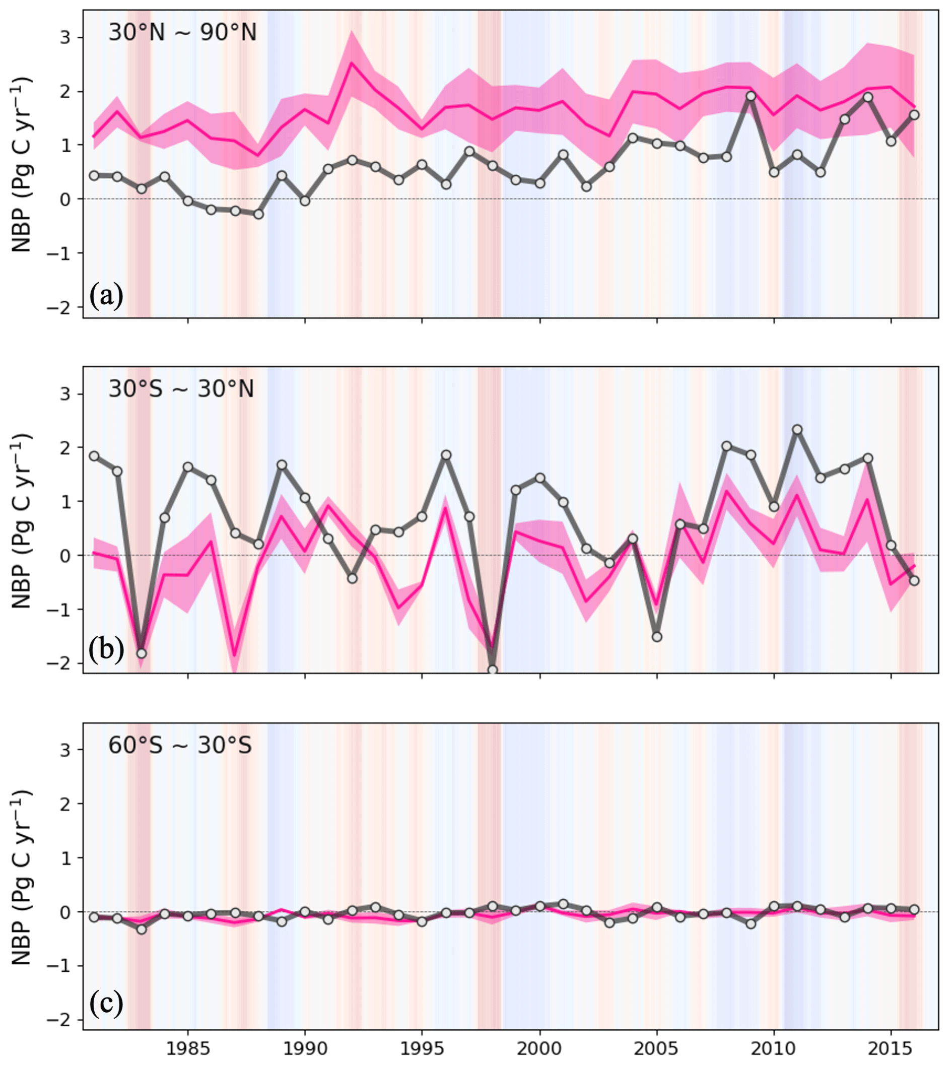
Figure 10Annual NBP between 1981 and 2016 from ED, and ensemble of atmospheric inversions for the Northern Hemisphere (>30∘ N) (a), tropics (30∘ N–30∘ S) (b) and the Southern Hemisphere (<30∘ S) (c). Black line is ED and the pink line and pink shading are the inversion ensemble average and the ±1σ spread of atmospheric inversions, respectively.
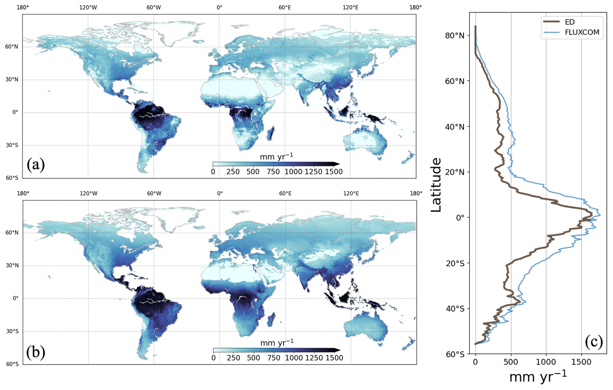
Figure 11Average annual ET between 1981 and 2016 from ED (a) and FLUXCOM (b), with a comparison of the corresponding latitudinal averages (c).
Globally, the ED estimate of global mean annual ET between 1981 and 2014 was 393.46 mm yr−1, which can be compared to 582.10 mm yr−1 from FLUXCOM. ED estimates of ET were also compared to gridded FLUXCOM data and to FLUXCOM data by latitude (Fig. 11). Similar to the reference dataset, ED estimated the highest rates across the tropics, with decreases towards high latitudes. This pattern generally followed the spatial distribution of precipitation. ED estimates were close to FLUXCOM over the tropics (i.e., 1500 mm yr−1) as well as latitudes above 60∘ N and below 35∘ S (i.e., below 500 mm yr−1), but notably underestimated average annual ET in other latitudes. ED estimates were generally smaller than FLUXCOM in dry regions such as southern Africa and interior Australia.
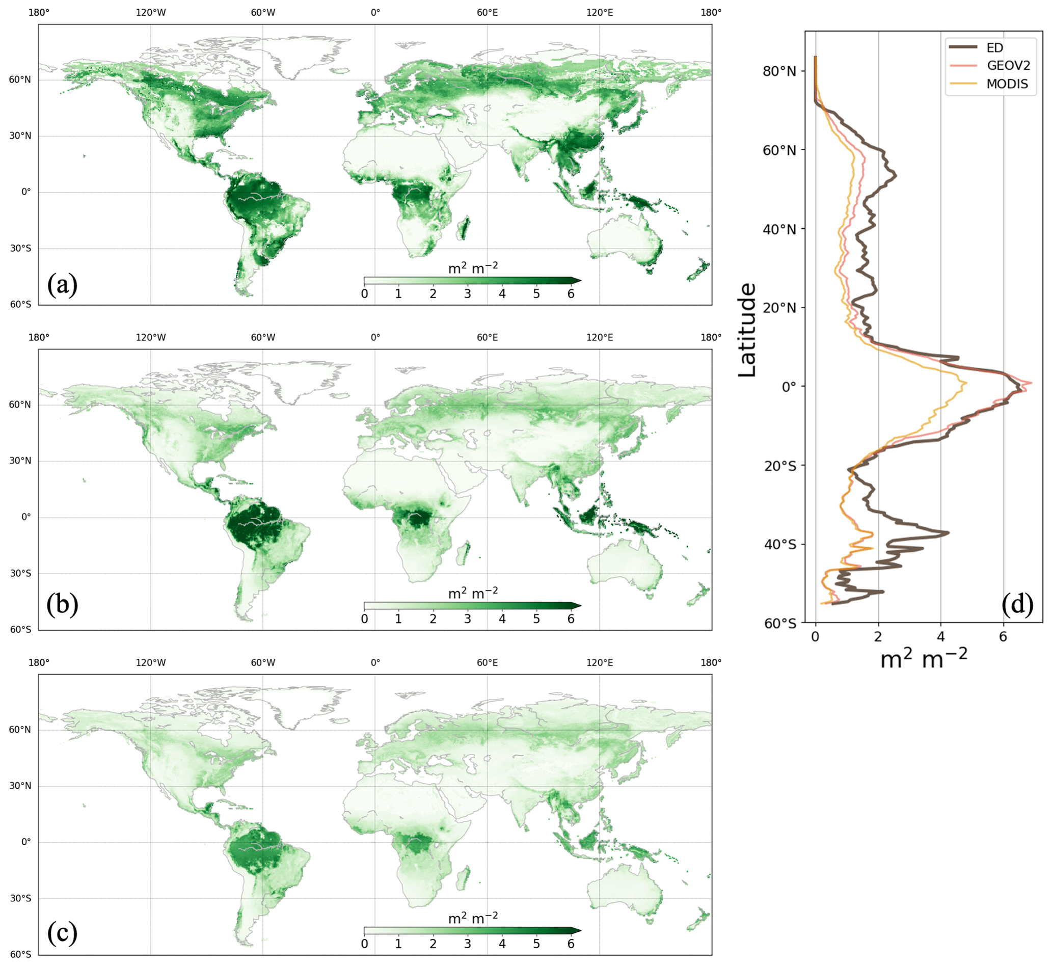
Figure 12Average LAI during the growing season between 2003 and 2016 from ED (a), GEOV2 (b) and MODIS (c). Corresponding latitudinal averages are compared in (d). Growing season is defined as the months during which the average air temperature of MERRA2 is above 0 ∘C.
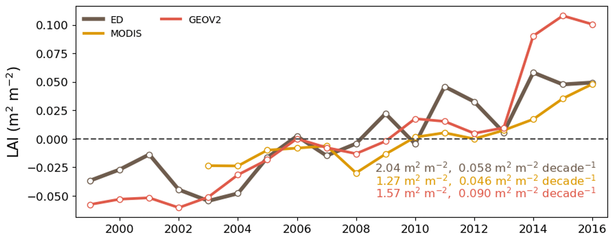
Figure 13Interannual global average growing season LAI from ED, MODIS and GEOV2. The anomaly is calculated by subtracting the multi-year average from the annual LAI.
3.4 Evaluation of canopy height and LAI vertical profile
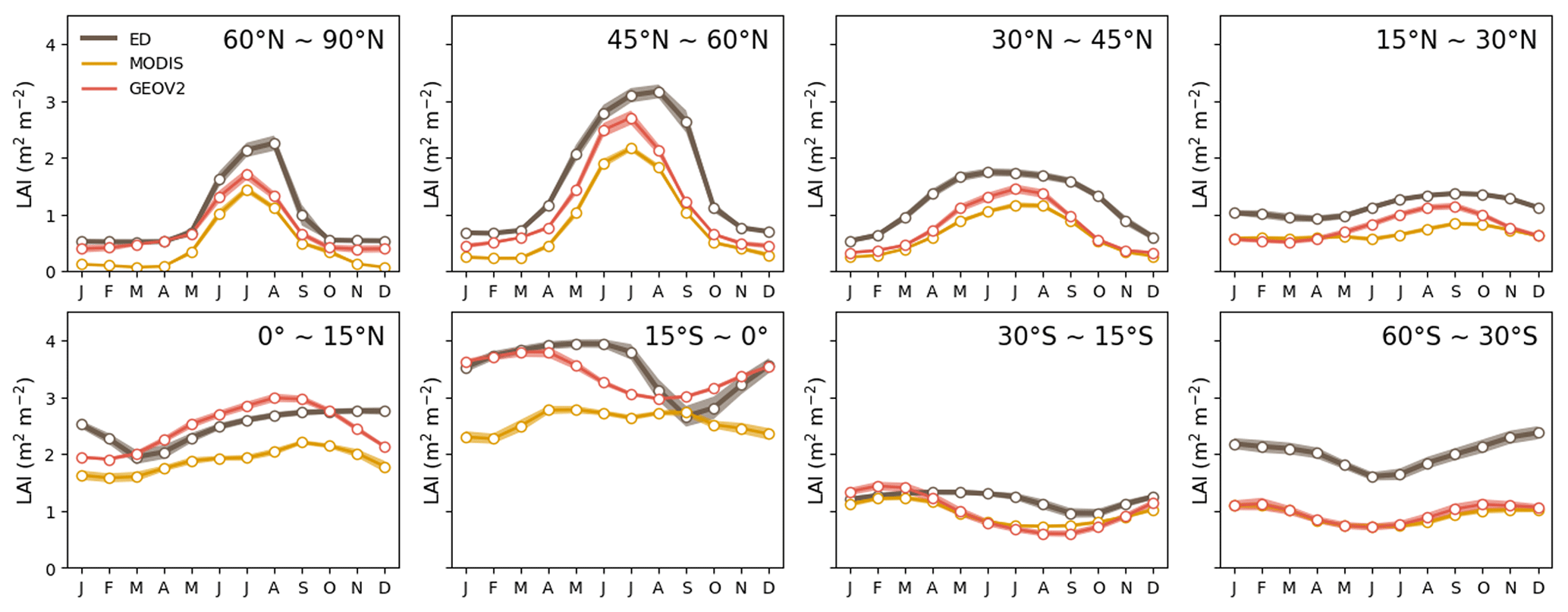
Evaluation of vegetation structure estimates focused on leaf area and canopy height. Figure 12 presents the spatial distribution of growing-season LAI from ED, GEOV2 and MODIS. Growing-season LAI was chosen for comparison because winter snow in the northern region (e.g., boreal forests) might affect LAI retrieval and cause uncertainties in remote sensing estimates (Murray-Tortarolo et al., 2013). There was good agreement in spatial pattern between ED and reference LAIs (Fig. 12d); the pattern showed peaks in the tropics and boreal region (near 50∘ N) and relatively low estimates across temperate regions. In the tropics, ED estimated an average LAI of 6.0 m2 m−2, which was similar to GEOV2 but higher than MODIS. However, ED produced higher LAI in temperate and boreal regions than both reference datasets, specifically in southern China and Brazil. Despite these differences, there was a general agreement in the greening trend between 1999 and 2016 (as shown in Fig. 13). The linear-fitted LAI trend was 0.058 m2 m−2 per decade for ED, 0.090 m2 m−2 for GEOV2, and 0.046 m2 m−2 for MODIS. LAI seasonality is also compared across latitudinal bands in Fig. 14. Similar to the references, ED captures the peak season in latitudinal bands 60–90∘ N, 45–60∘ N and 60–30∘ S, but shows less agreement with the references in the tropics (0–15∘ N and 15∘ S–0∘). In addition, ED LAI is larger than either reference LAI in winter; also, at latitudes above 45∘ N, and between 30 and 45∘ N, ED LAI is higher in all seasons. Similarly, there is higher LAI at 60–30∘ S, across southern China and Brazil.
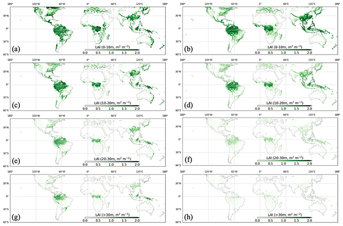
Figure 15Vertical LAI from ED (left column) and GEDI L2B (right column) at heights of 0–10 m in (a) and (b), 10–20 m in (c) and (d), 20–30 m in (e) and (f), and above 30 m in (g) and (h).
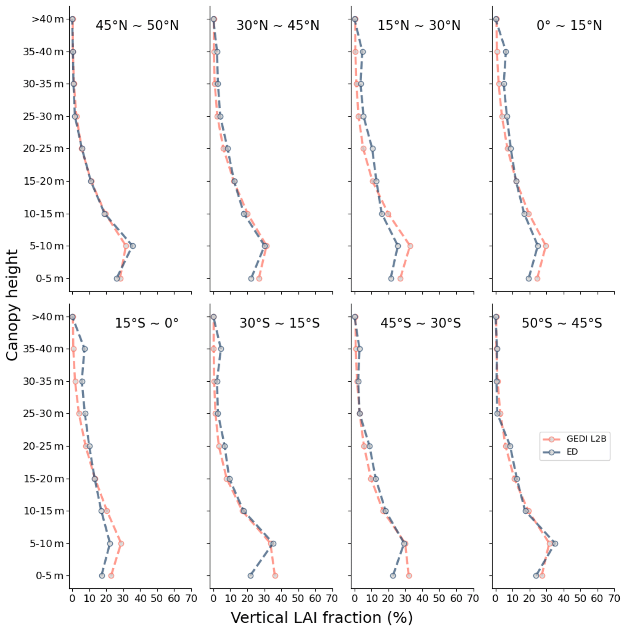
The estimated vertical profile of LAI from ED was compared to that from GEDI both spatially and latitudinally. Spatially, ED and GEDI L2B had similar spatial patterns, with most vegetated regions having concentrated LAI values under 10 m, and only tropical forests, part of southern China and the US having substantial LAI values above 30 m (Fig. 15). Comparisons of LAI profiles by latitude band indicate close agreement in each zone, with all regions having the highest values of LAI closest to the ground (0–5 and 5–10 m), and LAI decreasing with canopy height (Fig. 16). Discrepancies can be seen at the 0–5 m interval in the latitudinal bands 30–15∘ S and 45–30∘ S, where ED tends to be higher.
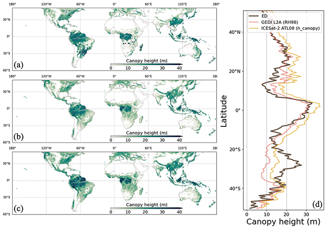
Figure 17Canopy height from ED (a), GEDI L2A (b) and ICESat-2 ATL08 (c). Latitudinal averages are compared in (d). ESA CCI data grids with tree fractions below 5 % are masked.
Tree canopy height estimates from ED were compared with satellite lidar observations from GEDI and ICESat-2 (Fig. 17). Like the reference datasets, ED produced a spatial pattern with taller trees in tropical rainforests, southern China and the eastern US. The canopy height gradient from forests to savannas in South America (northwest to southeast) and in Africa (central to north and south) were also generally captured by ED. A latitudinal comparison shows that the ED estimated average height is above 30 m in the tropics and ∼10 m in temperate regions. The general differences between the ED and reference datasets are less than 10 m across all latitudes. However, ED tree height in southern China and Brazil was higher than those from the references, and was lower than those from the references across African savanna.
Previous studies have developed benchmarking packages and designed model intercomparison activities to evaluate model performance (Abramowitz, 2012; Collier et al., 2018; Eyring et al., 2016; Ghimire et al., 2016; Luo et al., 2012; Randerson et al., 2009; Sitch et al., 2008). Like those studies, we evaluated ED model results using many key datasets and variables. This work utilized a particularly wide range of variables, including the latest versions of key forcing data on climate and land use and added a new focus on vegetation structure.
ED v3.0 includes modifications in four major areas (i.e., PFT representation, leaf-level physiology, hydrology and wood products) to improve model performance at the global scale. These modifications have several qualitative benefits. The refinement of PFTs provides a more complete representation of global vegetation functional types spanning from deciduous to evergreen, from broadleaf to needleleaf, from C3 to C4, and from softwood to hardwood. Updated temperature dependence functions in the leaf physiology submodule provide improved calibration and validation with independent field studies. The hydrology submodule now includes characterization of evaporation and snow, which was missing in previous regional versions. The land-use submodule now includes a wood product pool that facilitates tracking of the magnitude and timing of vegetation carbon loss and emissions due to deforestation and wood harvesting. These modifications also led to improved quantitative performance against a range of important benchmarks.
ED estimation of carbon stocks and fluxes compared favorably to benchmarking datasets across a range of spatial and temporal scales, from grid cell to global and from seasonal to decadal. Similar to benchmarking datasets, ED reproduced latitudinal gradients of GPP and AGB, a positive trend in global total GPP, global total AGB and GPP within reference ranges, and the interannual variation of NBP in response to El Niño and La Niña events. Producing such patterns of global carbon fluxes and stocks is challenging, as it requires models to have the ability to mechanistically scale up physiological processes from the leaf to ecosystem scale. It also requires models to accurately characterize responses of ecosystem demographic processes to climate change, soil conditions, and land-use activities. As a part of a new generation of DGVMs attempting to meet these challenges, ED leverages advances in the understanding of ecosystem physiology (e.g., the Ball–Berry stomatal conductance model and Farquhar photosynthesis model) (Ball et al., 1987; Farquhar et al., 1980), soil biogeochemistry (e.g., the CENTURY soil model) (Parton, 1996), and disturbance and recovery processes (e.g., LUH1/LUH2 modeling of land-use transition through time) (Hurtt et al., 2011, 2020).
In addition to carbon stocks and fluxes, ED simultaneously estimated the spatial distribution of seven major PFTs globally. ED reproduced the dominance of broadleaf PFTs in tropics and needleleaf PFTs at high latitudes, which is similar to benchmarking data. The ability to estimate these patterns mechanistically required the ability to characterize functional plant traits and trade-offs of vegetation as well as the processes and timescales of competition for light, water and other resources. Numerous studies have made advances that have contributed to the progress made in this study. For example, plant traits have been observed and compiled across a wide range of species and geographical domains (Reich et al., 1997; Kattge et al., 2011, 2020). Individual-based/gap models have been developed to track the life cycle of each individual tree and competition between individuals at the plot and site levels (Botkin et al., 1972; Shugart and West, 1977; Shugart et al., 2018; Pacala et al., 1996). Meanwhile, the SAS scaling approach was developed to efficiently scale up the individual scale to ecosystem dynamics at regional and continental scales (Hurtt et al., 1998; Moorcroft et al., 2001).
ED estimation of vegetation structure was also evaluated against benchmark data; in this case, novel observations from lidar remote-sensing data. Impressively, ED mechanistically and independently produced latitudinal mean height and LAI profiles similar to benchmarking datasets on vegetation structure. This progress is perhaps the most novel achievement because progress on this topic was previously limited due to a lack of global observations of vegetation structure. Importantly, the ED model is natively height structured, in that all trees have explicit heights. Originally, this feature was included to enable the simulation of individual-based competition for light. This feature, however, also offers the potential for a direct connection to lidar observations on vegetation structure for the purpose of model validation and/or initialization. Numerous studies have been completed at local and regional scales by initializing the ED model with airborne lidar data, demonstrating the power of the lidar technique to improve the characterization of contemporary ecosystem conditions (Hurtt et al., 2004, 2010, 2016, 2019a; Ma et al., 2021b). The advent of GEDI (Dubayah et al., 2020a) and ICESat-2 (Markus et al., 2017) has now expanded the potential for model evaluation and initialization to global scales.
Despite all of these advances, there are several important examples of differences between ED estimates and reference values that present important challenges for the future. First, ED estimates of AGB/GPP exceeded reference values in some regions, most notably southern China, southeast Asia and southeast Brazil. Correspondingly, ED also tended to overestimate tree height in those regions. The discrepancies share a similar spatial pattern and are likely interrelated. One hypothesis is that this overestimation may result, at least in part, from the land-use forcing. LUH2 has been shown to underestimate harvesting area in primary forest for the period after 1950 for both southern China and Southeast Asia, and it underestimates total cropland area in Brazil (Chini et al., 2021). LUH2 is being continuously updated and improved through its contribution to the Global Carbon Budget project (Chini et al., 2021). Second, while relative patterns for soil carbon showed close agreement at the biome level for the majority of biomes, the absolute magnitude of soil carbon was much lower than reference for several biomes and thus globally. Before overinterpreting these differences, it should be noted that there are substantial uncertainties with current empirical soil carbon maps in terms of both global totals and the spatial distribution (Todd-Brown et al., 2013). Model errors in soil carbon may arise from poor representations of biophysical conditions, inaccurate parameterization, or a lack of other important drivers. The representation of soil carbon in ED, like that in many other DGVMs/ESMs, is highly simplified, and the relatively low soil carbon is consistent with a relatively short residence time of soil carbon (about 11.4 years), which was close to the lower bound of other CMIP6 ESMs (Ito et al., 2020). Third, ED estimates of ET were lower than reference across all latitudes. One reason for this difference could be the parameterization of Penman–Monteith equations in the Hydrology submodule, as the value of aerodynamic resistance used in this study was higher than reported in Mu et al. (2011). A second potential cause could be the scaling of evapotranspiration (Bonan et al., 2021), which combines cohort-scale transpiration with patch-scale evaporation and currently omits the vertical variation of evaporation. Finally, the seasonality of GPP and LAI in the tropics differed from reference datasets. The pattern and timing of seasonality in the tropics is scientifically challenging to understand and has been the subject of several recent studies (Morton et al., 2014; Saleska et al., 2016; Tang and Dubayah, 2017). In ED, similar to other DGVMs/ESMs, soil water availability is assumed to be the primary driver of tropical phenology. Such mechanisms lead to reduced LAI and GPP in dry seasons, which contrasts with observations (Restrepo-Coupe et al., 2017).
Historically, different models have been developed separately in areas of biogeochemistry, biogeography and biophysics, and in some cases important patterns have been established through observations or other prior constraints (Bonan, 1994; Dickinson et al., 1993; Haxeltine and Prentice, 1996; Hurtt et al., 1998; Lieth, 1975; Neilson, 1995; Parton, 1996; Potter et al., 1993; Prentice et al., 1992; Raich et al., 1991; Sellers et al., 1986). The ability of this model to reliably simulate such a wide range of phenomena globally in a single mechanistic and consistent framework represents an important interdisciplinary synthesis and a functional modeling advance, and is, to our knowledge, unprecedented. Future work will focus on addressing the limitations discussed above and making direct connections with lidar forest structure observations from GEDI and ICESat-2 to improve demographic processes and the quantification and attribution of the terrestrial carbon cycle. Meanwhile, the global development and evaluation of ED demonstrates the model's ability to characterize essential aspects of terrestrial vegetation dynamics and the carbon cycle for a range of important applications. This model has recently been integrated with NASA's Goddard Earth Observing System, Version 5 (GEOS-5) to forecast seasonal biosphere–atmosphere CO2 fluxes in the 2015–2016 El Niño (Ott et al., 2018), used in NASA's Carbon Monitoring System as the tool for high spatial resolution (e.g., 90 m) regional forest carbon modeling and monitoring (Hurtt et al., 2019b; Ma et al., 2021b), and leveraged by NASA's Global Ecosystem Dynamics Investigation mission for the quantification of land carbon sequestration potential (Dubayah et al., 2020a; Ma et al., 2020). Results from these studies will likely be of importance for a range of scientific applications and will be used to inform and prioritize future model advances. Meanwhile, the increasing number of remote sensing missions and related datasets, advances in computation, and growing stakeholder interests in carbon and the climate, as evidenced by the UN Paris Climate Agreement, bode well for future advances.
All model simulation and source scripts can be found in https://doi.org/10.5281/zenodo.5236771 (Ma et al., 2021a). All benchmarking datasets are cited and publicly available.
The supplement related to this article is available online at: https://doi.org/10.5194/gmd-15-1971-2022-supplement.
LM, GH, JF, SF and RS developed the model code. LM, GH and LO designed this study. LM conducted the model simulation and evaluation. LM, GH and RL wrote the main body of the paper. All authors contributed to the analysis and paper preparation.
The contact author has declared that neither they nor their co-authors have any competing interests.
Publisher's note: Copernicus Publications remains neutral with regard to jurisdictional claims in published maps and institutional affiliations.
We would like to thank the editor Hisashi Sato for the help and handling of the paper at various stages, and we also thank the anonymous reviewers for their constructive comments which significantly contributed to improve the paper.
This work was funded by NASA-CMS (grant nos. 80NSSC17K0710, 80NSSC20K0006 and 80NSSC21K1059) and NASA-IDS (grant no. 80NSSC17K0348).
This paper was edited by Hisashi Sato and reviewed by two anonymous referees.
Abramowitz, G.: Towards a public, standardized, diagnostic benchmarking system for land surface models, Geosci. Model Dev., 5, 819–827, https://doi.org/10.5194/gmd-5-819-2012, 2012.
Albani, M., Medvigy, D., Hurtt, G. C., and Moorcroft, P. R.: The contributions of land-use change, CO2 fertilization, and climate variability to the Eastern US carbon sink, Global Change Biology, 12, 2370–2390, https://doi.org/10.1111/j.1365-2486.2006.01254.x, 2006.
Anav, A., Friedlingstein, P., Kidston, M., Bopp, L., Ciais, P., Cox, P., Jones, C., Jung, M., Myneni, R., and Zhu, Z.: Evaluating the land and ocean components of the global carbon cycle in the CMIP5 earth system models, J. Climate, 26, 6801–6843, https://doi.org/10.1175/JCLI-D-12-00417.1, 2013.
Ball, J. T., Woodrow, I. E., and Berry, J. A.: A model predicting stomatal conductance and its contribution to the control of photosynthesis under different environmental conditions, in: Progress in photosynthesis research, https://doi.org/10.1007/978-94-017-0519-6_48, Springer, 221–224, 1987.
Beer, C., Reichstein, M., Tomelleri, E., Ciais, P., Jung, M., Carvalhais, N., Rödenbeck, C., Arain, M. A., Baldocchi, D., Bonan, G. B., Bondeau, A., Cescatti, A., Lasslop, G., Lindroth, A., Lomas, M., Luyssaert, S., Margolis, H., Oleson, K. W., Roupsard, O., Veenendaal, E., Viovy, N., Williams, C., Woodward, F. I., and Papale, D.: Terrestrial Gross Carbon Dioxide Uptake: Global Distribution and Covariation with Climate, Science, 329, 834, https://doi.org/10.1126/science.1184984, 2010.
Bernacchi, C. J., Singsaas, E. L., Pimentel Jr., C. A. R. P., and Long, S. P.: Improved temperature response functions for models of Rubisco-limited photosynthesis, Plant Cell Environ., 24, 253–259, https://doi.org/10.1111/j.1365-3040.2001.00668.x, 2001.
Bonan, G. B.: Comparison of two land surface process models using prescribed forcings, J. Geographys. Res.-Atmos., 99, 25803–25818, https://doi.org/10.1029/94JD02188, 1994.
Bonan, G. B., Patton, E. G., Finnigan, J. J., Baldocchi, D. D., and Harman, I. N.: Moving beyond the incorrect but useful paradigm: reevaluating big-leaf and multilayer plant canopies to model biosphere-atmosphere fluxes – a review, Agric. Forest Meteorol., 306, 108435, https://doi.org/10.1016/j.agrformet.2021.108435, 2021.
Botkin, D. B., Janak, J. F., and Wallis, J. R.: Some ecological consequences of a computer model of forest growth, J. Ecol., 60, 849–872, 1972.
Brovkin, V., Sitch, S., Von Bloh, W., Claussen, M., Bauer, E., and Cramer, W.: Role of land cover changes for atmospheric CO2 increase and climate change during the last 150 years, Global Change Biol., 10, 1253–1266, https://doi.org/10.1111/j.1365-2486.2004.00812.x, 2004.
Canadell, J. G., Kirschbaum, M. U. F., Kurz, W. A., Sanz, M.-J., Schlamadinger, B., and Yamagata, Y.: Factoring out natural and indirect human effects on terrestrial carbon sources and sinks, Environ. Sci. Policy, 10, 370–384, https://doi.org/10.1016/j.envsci.2007.01.009, 2007.
Chevallier, F., Fisher, M., Peylin, P., Serrar, S., Bousquet, P., Bréon, F.-M., Chédin, A., and Ciais, P.: Inferring CO2 sources and sinks from satellite observations: Method and application to TOVS data, J. Geophys. Res., 110, D24309, https://doi.org/10.1029/2005JD006390, 2005.
Chini, L., Hurtt, G., Sahajpal, R., Frolking, S., Klein Goldewijk, K., Sitch, S., Ganzenmüller, R., Ma, L., Ott, L., Pongratz, J., and Poulter, B.: Land-use harmonization datasets for annual global carbon budgets, Earth Syst. Sci. Data, 13, 4175–4189, https://doi.org/10.5194/essd-13-4175-2021, 2021.
Ciais, P., Dolman, A. J., Bombelli, A., Duren, R., Peregon, A., Rayner, P. J., Miller, C., Gobron, N., Kinderman, G., Marland, G., Gruber, N., Chevallier, F., Andres, R. J., Balsamo, G., Bopp, L., Bréon, F.-M., Broquet, G., Dargaville, R., Battin, T. J., Borges, A., Bovensmann, H., Buchwitz, M., Butler, J., Canadell, J. G., Cook, R. B., DeFries, R., Engelen, R., Gurney, K. R., Heinze, C., Heimann, M., Held, A., Henry, M., Law, B., Luyssaert, S., Miller, J., Moriyama, T., Moulin, C., Myneni, R. B., Nussli, C., Obersteiner, M., Ojima, D., Pan, Y., Paris, J.-D., Piao, S. L., Poulter, B., Plummer, S., Quegan, S., Raymond, P., Reichstein, M., Rivier, L., Sabine, C., Schimel, D., Tarasova, O., Valentini, R., Wang, R., van der Werf, G., Wickland, D., Williams, M., and Zehner, C.: Current systematic carbon-cycle observations and the need for implementing a policy-relevant carbon observing system, Biogeosciences, 11, 3547–3602, https://doi.org/10.5194/bg-11-3547-2014, 2014a.
Ciais, P., Sabine, C., Bala, G., Bopp, L., Brovkin, V., Canadell, J., Chhabra, A., DeFries, R., Galloway, J., and Heimann, M.: Carbon and other biogeochemical cycles, in Climate change 2013: the physical science basis. Contribution of Working Group I to the Fifth Assessment Report of the Intergovernmental Panel on Climate Change, 465–570, Cambridge University Press, https://doi.org/10.1017/CBO9781107415324.015, 2014b.
Collatz, G. J., Ball, J. T., Grivet, C., and Berry, J. A.: Physiological and environmental regulation of stomatal conductance, photosynthesis and transpiration: a model that includes a laminar boundary layer, Agric. Forest Meteorol., 54, 107–136, https://doi.org/10.1016/0168-1923(91)90002-8, 1991.
Collatz, G. J., Ribas-Carbo, M., and Berry, J. A.: Coupled photosynthesis-stomatal conductance model for leaves of C4 plants, Aust. J. Plant Physiol., 19, 519–538, https://doi.org/10.1071/PP9920519, 1992.
Collier, N., Hoffman, F. M., Lawrence, D. M., Keppel-Aleks, G., Koven, C. D., Riley, W. J., Mu, M., and Randerson, J. T.: The International Land Model Benchmarking (ILAMB) System: Design, Theory, and Implementation, J. Adv. Model. Earth Sy., 10, 2731–2754, https://doi.org/10.1029/2018MS001354, 2018.
Cramer, W., Bondeau, A., Woodward, F. I., Prentice, I. C., Betts, R. A., Brovkin, V., Cox, P. M., Fisher, V., Foley, J. A., Friend, A. D., Kucharik, C., Lomas, M. R., Ramankutty, N., Sitch, S., Smith, B., White, A., and Young-Molling, C.: Global response of terrestrial ecosystem structure and function to CO2 and climate change: results from six dynamic global vegetation models, Global Change Biol., 7, 357–373, https://doi.org/10.1046/j.1365-2486.2001.00383.x, 2001.
Dickinson, R. E., Henderson-Sellers, A., and Kennedy, P. J.: Biosphere-atmosphere Transfer Scheme (BATS) Version 1e as Coupled to the NCAR Community Climate Model (No. NCAR/TN-387+STR), University Corporation for Atmospheric Research, https://doi.org/10.5065/D67W6959, 1993.
Dubayah, R., Blair, J. B., Goetz, S., Fatoyinbo, L., Hansen, M., Healey, S., Hofton, M., Hurtt, G., Kellner, J., Luthcke, S., Armston, J., Tang, H., Duncanson, L., Hancock, S., Jantz, P., Marselis, S., Patterson, P. L., Qi, W., and Silva, C.: The Global Ecosystem Dynamics Investigation: High-resolution laser ranging of the Earth's forests and topography, Sci. Remote Sens., 1, 100002, https://doi.org/10.1016/j.srs.2020.100002, 2020a.
Dubayah, R., Hofton, M., Blair, J., Armston, J., Tang, H., and Luthcke, S.: GEDI L2A Elevation and Height Metrics Data Global Footprint Level V001, NASA Earth Data, https://doi.org/10.5067/GEDI/GEDI02_A.001, 2020b.
Dubayah, R., Tang, H., Armston, J., Luthcke, S., Hofton, M., and Blair, J.: GEDI L2B Canopy Cover and Vertical Profile Metrics Data Global Footprint Level V001, NASA Earth Data, https://doi.org/10.5067/GEDI/GEDI02_B.001, 2020c.
Erb, K.-H., Kastner, T., Luyssaert, S., Houghton, R. A., Kuemmerle, T., Olofsson, P., and Haberl, H.: Bias in the attribution of forest carbon sinks, Nat. Clim. Change, 3, 854–856, https://doi.org/10.1038/nclimate2004, 2013.
ESA: Land Cover CCI Product User Guide Version 2, Tech. Rep., http://maps.elie.ucl.ac.be/CCI/viewer/download/ESACCI-LC-Ph2-PUGv2_2.0.pdf (last access: 1 March 2022), 2017.
Eyring, V., Gleckler, P. J., Heinze, C., Stouffer, R. J., Taylor, K. E., Balaji, V., Guilyardi, E., Joussaume, S., Kindermann, S., Lawrence, B. N., Meehl, G. A., Righi, M., and Williams, D. N.: Towards improved and more routine Earth system model evaluation in CMIP, Earth Syst. Dynam., 7, 813–830, https://doi.org/10.5194/esd-7-813-2016, 2016.
Eyring, V., Cox, P. M., Flato, G. M., Gleckler, P. J., Abramowitz, G., Caldwell, P., Collins, W. D., Gier, B. K., Hall, A. D., Hoffman, F. M., Hurtt, G. C., Jahn, A., Jones, C. D., Klein, S. A., Krasting, J. P., Kwiatkowski, L., Lorenz, R., Maloney, E., Meehl, G. A., Pendergrass, A. G., Pincus, R., Ruane, A. C., Russell, J. L., Sanderson, B. M., Santer, B. D., Sherwood, S. C., Simpson, I. R., Stouffer, R. J., and Williamson, M. S.: Taking climate model evaluation to the next level, Nat. Clim. Change, 9, 102–110, https://doi.org/10.1038/s41558-018-0355-y, 2019.
Farjon, A. and Filer, D.: An Atlas of the World's Conifers: An Analysis of their Distribution, Biogeography, Diversity and Conservation Status, Brill, https://brill.com/view/title/20587 (last access: 22 December 2020), 2013.
Farquhar, G. D. and Sharkey, T. D.: Stomatal conductance and photosynthesis, Annu. Rev. Plant Physiol., 33, 317–345, https://doi.org/10.1146/annurev.pp.33.060182.001533, 1982.
Farquhar, G. D., von Caemmerer, S., and Berry, J. A.: A biochemical model of photosynthetic CO2 assimilation in leaves of C3 species, Planta, 149, 78–90, https://doi.org/10.1007/BF00386231, 1980.
Fisher, R. A., Muszala, S., Verteinstein, M., Lawrence, P., Xu, C., McDowell, N. G., Knox, R. G., Koven, C., Holm, J., Rogers, B. M., Spessa, A., Lawrence, D., and Bonan, G.: Taking off the training wheels: the properties of a dynamic vegetation model without climate envelopes, CLM4.5(ED), Geosci. Model Dev., 8, 3593–3619, https://doi.org/10.5194/gmd-8-3593-2015, 2015.
Fisher, R. A., Koven, C. D., Anderegg, W. R. L., Christoffersen, B. O., Dietze, M. C., Farrior, C. E., Holm, J. A., Hurtt, G. C., Knox, R. G., Lawrence, P. J., Lichstein, J. W., Longo, M., Matheny, A. M., Medvigy, D., Muller-Landau, H. C., Powell, T. L., Serbin, S. P., Sato, H., Shuman, J. K., Smith, B., Trugman, A. T., Viskari, T., Verbeeck, H., Weng, E., Xu, C., Xu, X., Zhang, T., and Moorcroft, P. R.: Vegetation demographics in Earth System Models: A review of progress and priorities, Global Change Biol., 24, 35–54, https://doi.org/10.1111/gcb.13910, 2018.
Fisk, J. P.: Net effects of disturbance: Spatial, temporal, and soci-etal dimensions of forest disturbance and recovery on terrestrial carbon balance, PhD thesis, University of Maryland, College Park, Maryland, 2015.
Fisk, J. P., Hurtt, G. C., Chambers, J. Q., Zeng, H., Dolan, K. A., and Negrón-Juárez, R. I.: The impacts of tropical cyclones on the net carbon balance of eastern US forests (1851–2000), Environ. Res. Lett., 8, 045017, https://doi.org/10.1088/1748-9326/8/4/045017, 2013.
Flanagan, S. A., Hurtt, G. C., Fisk, J. P., Sahajpal, R., Zhao, M., Dubayah, R., Hansen, M. C., Sullivan, J. H., and Collatz, G. J.: Potential Transient Response of Terrestrial Vegetation and Carbon in Northern North America from Climate Change, Climate, 7, 113, https://doi.org/10.3390/cli7090113, 2019.
Foley, J. A., Prentice, I. C., Ramankutty, N., Levis, S., Pollard, D., Sitch, S., and Haxeltine, A.: An integrated biosphere model of land surface processes, terrestrial carbon balance, and vegetation dynamics, Global Biogeochem. Cycles, 10, 603–628, https://doi.org/10.1029/96GB02692, 1996.
Friedlingstein, P., O'Sullivan, M., Jones, M. W., Andrew, R. M., Hauck, J., Olsen, A., Peters, G. P., Peters, W., Pongratz, J., Sitch, S., Le Quéré, C., Canadell, J. G., Ciais, P., Jackson, R. B., Alin, S., Aragão, L. E. O. C., Arneth, A., Arora, V., Bates, N. R., Becker, M., Benoit-Cattin, A., Bittig, H. C., Bopp, L., Bultan, S., Chandra, N., Chevallier, F., Chini, L. P., Evans, W., Florentie, L., Forster, P. M., Gasser, T., Gehlen, M., Gilfillan, D., Gkritzalis, T., Gregor, L., Gruber, N., Harris, I., Hartung, K., Haverd, V., Houghton, R. A., Ilyina, T., Jain, A. K., Joetzjer, E., Kadono, K., Kato, E., Kitidis, V., Korsbakken, J. I., Landschützer, P., Lefèvre, N., Lenton, A., Lienert, S., Liu, Z., Lombardozzi, D., Marland, G., Metzl, N., Munro, D. R., Nabel, J. E. M. S., Nakaoka, S.-I., Niwa, Y., O'Brien, K., Ono, T., Palmer, P. I., Pierrot, D., Poulter, B., Resplandy, L., Robertson, E., Rödenbeck, C., Schwinger, J., Séférian, R., Skjelvan, I., Smith, A. J. P., Sutton, A. J., Tanhua, T., Tans, P. P., Tian, H., Tilbrook, B., van der Werf, G., Vuichard, N., Walker, A. P., Wanninkhof, R., Watson, A. J., Willis, D., Wiltshire, A. J., Yuan, W., Yue, X., and Zaehle, S.: Global Carbon Budget 2020, Earth Syst. Sci. Data, 12, 3269–3340, https://doi.org/10.5194/essd-12-3269-2020, 2020.
Gelaro, R., McCarty, W., Suárez, M. J., Todling, R., Molod, A., Takacs, L., Randles, C. A., Darmenov, A., Bosilovich, M. G., Reichle, R., Wargan, K., Coy, L., Cullather, R., Draper, C., Akella, S., Buchard, V., Conaty, A., da Silva, A. M., Gu, W., Kim, G.-K., Koster, R., Lucchesi, R., Merkova, D., Nielsen, J. E., Partyka, G., Pawson, S., Putman, W., Rienecker, M., Schubert, S. D., Sienkiewicz, M., and Zhao, B.: The Modern-Era Retrospective Analysis for Research and Applications, Version 2 (MERRA-2), J. Climate, 30, 5419–5454, https://doi.org/10.1175/JCLI-D-16-0758.1, 2017.
Ghimire, B., Riley, W. J., Koven, C. D., Mu, M., and Randerson, J. T.: Representing leaf and root physiological traits in CLM improves global carbon and nitrogen cycling predictions, J. Adv. Model. Earth Sy., 8, 598–613, https://doi.org/10.1002/2015MS000538, 2016.
Guanter, L., Zhang, Y., Jung, M., Joiner, J., Voigt, M., Berry, J. A., Frankenberg, C., Huete, A. R., Zarco-Tejada, P., Lee, J.-E., Moran, M. S., Ponce-Campos, G., Beer, C., Camps-Valls, G., Buchmann, N., Gianelle, D., Klumpp, K., Cescatti, A., Baker, J. M., and Griffis, T. J.: Global and time-resolved monitoring of crop photosynthesis with chlorophyll fluorescence, P. Natl. Acad. Sci. USA, 111, E1327–E1333, https://doi.org/10.1073/pnas.1320008111, 2014.
Hansis, E., Davis, S. J., and Pongratz, J.: Relevance of methodological choices for accounting of land use change carbon fluxes, Global Biogeochem. Cycles, 29, 1230–1246, https://doi.org/10.1002/2014GB004997, 2015.
Haxeltine, A. and Prentice, I. C.: BIOME3: An equilibrium terrestrial biosphere model based on ecophysiological constraints, resource availability, and competition among plant functional types, Global Biogeochem. Cycles, 10, 693–709, 1996.
Hurtt, G. C., Moorcroft, P. R., Pacala, S. W., and Levin, S. A.: Terrestrial models and global change: challenges for the future, Global Change Biol., 4, 581–590, https://doi.org/10.1046/j.1365-2486.1998.t01-1-00203.x, 1998.
Hurtt, G. C., Pacala, S. W., Moorcroft, P. R., Caspersen, J., Shevliakova, E., Houghton, R. A., and Moore, B.: Projecting the future of the U.S. carbon sink, P. Natl. Acad. Sci. USA, 99, 1389–1394, https://doi.org/10.1073/pnas.012249999, 2002.
Hurtt, G. C., Dubayah, R., Drake, J., Moorcroft, P. R., Pacala, S. W., Blair, J. B., and Fearon, M. G.: Beyond Potential Vegetation: Combining Lidar Data and a Height-Structured Model for Carbon Studies, Ecol. Appl., 14, 873–883, https://doi.org/10.1890/02-5317, 2004.
Hurtt, G. C., Fisk, J., Thomas, R. Q., Dubayah, R., Moorcroft, P. R., and Shugart, H. H.: Linking models and data on vegetation structure, J. Geophys. Res.-Biogeo., 115, G00E10, https://doi.org/10.1029/2009JG000937, 2010.
Hurtt, G. C., Chini, L. P., Frolking, S., Betts, R., Feddema, J., Fischer, G., Fisk, J., Hibbard, K., Houghton, R., and Janetos, A.: Harmonization of land-use scenarios for the period 1500–2100: 600 years of global gridded annual land-use transitions, wood harvest, and resulting secondary lands, Clim. Change, 109, 117–161, 2011.
Hurtt, G. C., Thomas, R. Q., Fisk, J. P., Dubayah, R. O., and Sheldon, S. L.: The Impact of Fine-Scale Disturbances on the Predictability of Vegetation Dynamics and Carbon Flux, PLOS ONE, 11, e0152883, https://doi.org/10.1371/journal.pone.0152883, 2016.
Hurtt, G. C., Chini, L., Sahajpal, R., Frolking, S., Bodirsky, B. L., Calvin, K., Doelman, J., Fisk, J., Fujimori, S., Goldewijk, K. K., Hasegawa, T., Havlik, P., Heinimann, A., Humpenöder, F., Jungclaus, J., Kaplan, J., Krisztin, T., Lawrence, D., Lawrence, P., Mertz, O., Pongratz, J., Popp, A., Riahi, K., Shevliakova, E., Stehfest, E., Thornton, P., van Vuuren, D., and Zhang, X.: input4MIPs.CMIP6.CMIP.UofMD, Earth System Grid Federation, https://doi.org/10.22033/ESGF/input4MIPs.10454, 2019a.
Hurtt, G. C., Zhao, M., Sahajpal, R., Armstrong, A., Birdsey, R., Campbell, E., Dolan, K., Dubayah, R., Fisk, J. P., Flanagan, S., Huang, C., Huang, W., Johnson, K., Lamb, R., Ma, L., Marks, R., O'Leary, D., O'Neil-Dunne, J., Swatantran, A., and Tang, H.: Beyond MRV: high-resolution forest carbon modeling for climate mitigation planning over Maryland, USA, Environ. Res. Lett., 14, 045013, https://doi.org/10.1088/1748-9326/ab0bbe, 2019b.
Hurtt, G. C., Chini, L., Sahajpal, R., Frolking, S., Bodirsky, B. L., Calvin, K., Doelman, J. C., Fisk, J., Fujimori, S., Klein Goldewijk, K., Hasegawa, T., Havlik, P., Heinimann, A., Humpenöder, F., Jungclaus, J., Kaplan, J. O., Kennedy, J., Krisztin, T., Lawrence, D., Lawrence, P., Ma, L., Mertz, O., Pongratz, J., Popp, A., Poulter, B., Riahi, K., Shevliakova, E., Stehfest, E., Thornton, P., Tubiello, F. N., van Vuuren, D. P., and Zhang, X.: Harmonization of global land use change and management for the period 850–2100 (LUH2) for CMIP6, Geosci. Model Dev., 13, 5425–5464, https://doi.org/10.5194/gmd-13-5425-2020, 2020.
Ito, A., Hajima, T., Lawrence, D. M., Brovkin, V., Delire, C., Guenet, B., Jones, C. D., Malyshev, S., Materia, S., McDermid, S. P., Peano, D., Pongratz, J., Robertson, E., Shevliakova, E., Vuichard, N., Wårlind, D., Wiltshire, A., and Ziehn, T.: Soil carbon sequestration simulated in CMIP6-LUMIP models: implications for climatic mitigation, Environ. Res. Lett., 15, 124061, https://doi.org/10.1088/1748-9326/abc912, 2020.
Joiner, J., Yoshida, Y., Zhang, Y., Duveiller, G., Jung, M., Lyapustin, A., Wang, Y., and Tucker, C. J.: Estimation of Terrestrial Global Gross Primary Production (GPP) with Satellite Data-Driven Models and Eddy Covariance Flux Data, Remote Sens., 10, 1346, https://doi.org/10.3390/rs10091346, 2018.
Jung, M., Schwalm, C., Migliavacca, M., Walther, S., Camps-Valls, G., Koirala, S., Anthoni, P., Besnard, S., Bodesheim, P., Carvalhais, N., Chevallier, F., Gans, F., Goll, D. S., Haverd, V., Köhler, P., Ichii, K., Jain, A. K., Liu, J., Lombardozzi, D., Nabel, J. E. M. S., Nelson, J. A., O'Sullivan, M., Pallandt, M., Papale, D., Peters, W., Pongratz, J., Rödenbeck, C., Sitch, S., Tramontana, G., Walker, A., Weber, U., and Reichstein, M.: Scaling carbon fluxes from eddy covariance sites to globe: synthesis and evaluation of the FLUXCOM approach, Biogeosciences, 17, 1343–1365, https://doi.org/10.5194/bg-17-1343-2020, 2020.
Kattge, J. and Knorr, W.: Temperature acclimation in a biochemical model of photosynthesis: a reanalysis of data from 36 species, Plant Cell Environ., 30, 1176–1190, https://doi.org/10.1111/j.1365-3040.2007.01690.x, 2007.
Kattge, J., Ogle, K., Bönisch, G., Díaz, S., Lavorel, S., Madin, J., Nadrowski, K., Nöllert, S., Sartor, K., and Wirth, C.: A generic structure for plant trait databases, Methods Ecol. Evol., 2, 202–213, https://doi.org/10.1111/j.2041-210X.2010.00067.x, 2011.
Kattge, J., Bönisch, G., Díaz, S., Lavorel, S., Prentice, I. C., Leadley, P., Tautenhahn, S., Werner, G. D., Aakala, T., and Abedi, M.: TRY plant trait database – enhanced coverage and open access, Global Change Biol., 26, 119–188, 2020.
Keeling, R. F.: Recording Earth's Vital Signs, Science, 319, 1771, https://doi.org/10.1126/science.1156761, 2008.
Keenan, T. F. and Williams, C. A.: The Terrestrial Carbon Sink, Annu. Rev. Environ. Resour., 43, 219–243, https://doi.org/10.1146/annurev-environ-102017-030204, 2018.
Lawrence, D. M., Fisher, R. A., Koven, C. D., Oleson, K. W., Swenson, S. C., Bonan, G., Collier, N., Ghimire, B., van Kampenhout, L., and Kennedy, D.: The Community Land Model version 5: Description of new features, benchmarking, and impact of forcing uncertainty, J. Adv. Model. Earth Sy., 11, 4245–4287, 2019.
Lee, J.-E., Frankenberg, C., van der Tol, C., Berry, J. A., Guanter, L., Boyce, C. K., Fisher, J. B., Morrow, E., Worden, J. R., Asefi, S., Badgley, G., and Saatchi, S.: Forest productivity and water stress in Amazonia: observations from GOSAT chlorophyll fluorescence, P. Roy. Soc. B, 280, 20130171, https://doi.org/10.1098/rspb.2013.0171, 2013.
Lieth, H.: Modeling the primary productivity of the world, in: Primary productivity of the biosphere, edited by: Lieth, H. and Whittaker, R. H., Springer, 237–263, https://doi.org/10.1007/978-3-642-80913-2, 1975.
Longo, M., Knox, R. G., Medvigy, D. M., Levine, N. M., Dietze, M. C., Kim, Y., Swann, A. L. S., Zhang, K., Rollinson, C. R., Bras, R. L., Wofsy, S. C., and Moorcroft, P. R.: The biophysics, ecology, and biogeochemistry of functionally diverse, vertically and horizontally heterogeneous ecosystems: the Ecosystem Demography model, version 2.2 – Part 1: Model description, Geosci. Model Dev., 12, 4309–4346, https://doi.org/10.5194/gmd-12-4309-2019, 2019.
Luo, Y. Q., Randerson, J. T., Abramowitz, G., Bacour, C., Blyth, E., Carvalhais, N., Ciais, P., Dalmonech, D., Fisher, J. B., Fisher, R., Friedlingstein, P., Hibbard, K., Hoffman, F., Huntzinger, D., Jones, C. D., Koven, C., Lawrence, D., Li, D. J., Mahecha, M., Niu, S. L., Norby, R., Piao, S. L., Qi, X., Peylin, P., Prentice, I. C., Riley, W., Reichstein, M., Schwalm, C., Wang, Y. P., Xia, J. Y., Zaehle, S., and Zhou, X. H.: A framework for benchmarking land models, Biogeosciences, 9, 3857–3874, https://doi.org/10.5194/bg-9-3857-2012, 2012.
Ma, L., Hurtt, G., Ott, L., Sahajpal, R., Fisk, J., Flanagan, S., Poulter, B., Liang, S., Sullivan, J., and Dubayah, R.: Global Ecosystem Demography Model (ED-global v1.0): Development, Calibration and Evaluation for NASA's Global Ecosystem Dynamics Investigation (GEDI), Earth and Space Science Open Archive, https://doi.org/10.1002/essoar.10505486.1, 2020.
Ma, L., Hurtt, G., Ott, L., Sahajpal, R., Fisk, J., Lamb, R., Tang, H., Flanagan, S., Chini, L., Chatterjee, A., and Sullivan, J.: Global evaluation of the Ecosystem Demography model (ED v3.0), Zenodo [code], https://doi.org/10.5281/zenodo.5236771, 2021a.
Ma, L., Hurtt, G., Tang, H., Lamb, R. L., Campbell, E., Dubayah, R. O., Guy, M., Huang, W., Lister, A., and Lu, J.: High-resolution forest carbon modeling for climate mitigation planning over the RGGI region, USA, Environ. Res. Lett., 16, 045014, https://doi.org/10.1088/1748-9326/abe4f4, 2021b.
Markus, T., Neumann, T., Martino, A., Abdalati, W., Brunt, K., Csatho, B., Farrell, S., Fricker, H., Gardner, A., Harding, D., Jasinski, M., Kwok, R., Magruder, L., Lubin, D., Luthcke, S., Morison, J., Nelson, R., Neuenschwander, A., Palm, S., Popescu, S., Shum, C., Schutz, B. E., Smith, B., Yang, Y., and Zwally, J.: The Ice, Cloud, and land Elevation Satellite-2 (ICESat-2): Science requirements, concept, and implementation, Remote Sens. Environ., 190, 260–273, https://doi.org/10.1016/j.rse.2016.12.029, 2017.
Massad, R.-S., Tuzet, A., and Bethenod, O.: The effect of temperature on C4-type leaf photosynthesis parameters, Plant Cell Environ., 30, 1191–1204, https://doi.org/10.1111/j.1365-3040.2007.01691.x, 2007.
Massoud, E. C., Xu, C., Fisher, R. A., Knox, R. G., Walker, A. P., Serbin, S. P., Christoffersen, B. O., Holm, J. A., Kueppers, L. M., Ricciuto, D. M., Wei, L., Johnson, D. J., Chambers, J. Q., Koven, C. D., McDowell, N. G., and Vrugt, J. A.: Identification of key parameters controlling demographically structured vegetation dynamics in a land surface model: CLM4.5(FATES), Geosci. Model Dev., 12, 4133–4164, https://doi.org/10.5194/gmd-12-4133-2019, 2019.
Medvigy, D.: The State of the Regional Carbon Cycle: Results from a Constrained Coupled Ecosystem-atmosphere Model, PhD thesis, Harvard University, Cambridge, Massachusetts, 644 pp., 2006.
Medvigy, D., Wofsy, S. C., Munger, J. W., Hollinger, D. Y., and Moorcroft, P. R.: Mechanistic scaling of ecosystem function and dynamics in space and time: Ecosystem Demography model version 2, J. Geophys. Res.-Biogeo., 114, G01002, https://doi.org/10.1029/2008JG000812, 2009.
Mercado, L. M., Bellouin, N., Sitch, S., Boucher, O., Huntingford, C., Wild, M., and Cox, P. M.: Impact of changes in diffuse radiation on the global land carbon sink, Nature, 458, 1014–1017, 2009.
Monteith, J.: Evaporation and environment, Symposia of the Society for Experimental Biology, 19, 205–234, 1965.
Montzka, C., Herbst, M., Weihermüller, L., Verhoef, A., and Vereecken, H.: A global data set of soil hydraulic properties and sub-grid variability of soil water retention and hydraulic conductivity curves, Earth Syst. Sci. Data, 9, 529–543, https://doi.org/10.5194/essd-9-529-2017, 2017.
Moorcroft, P. R., Hurtt, G. C., and Pacala, S. W.: A Method for Scaling Vegetation Dynamics: The Ecosystem Demography Model, Ecological Monographs, 71, 557–586, https://doi.org/10.1890/0012-9615(2001)071[0557:AMFSVD]2.0.CO;2, 2001.
Morton, D. C., Nagol, J., Carabajal, C. C., Rosette, J., Palace, M., Cook, B. D., Vermote, E. F., Harding, D. J., and North, P. R. J.: Amazon forests maintain consistent canopy structure and greenness during the dry season, Nature, 506, 221–224, https://doi.org/10.1038/nature13006, 2014.
Mu, Q., Zhao, M., and Running, S. W.: Improvements to a MODIS global terrestrial evapotranspiration algorithm, Remote Sens. Environ., 115, 1781–1800, 2011.
Murray-Tortarolo, G., Anav, A., Friedlingstein, P., Sitch, S., Piao, S., Zhu, Z., Poulter, B., Zaehle, S., Ahlström, A., Lomas, M., Levis, S., Viovy, N., and Zeng, N.: Evaluation of Land Surface Models in Reproducing Satellite-Derived LAI over the High-Latitude Northern Hemisphere. Part I: Uncoupled DGVMs, Remote Sens., 5, 4819–4838, https://doi.org/10.3390/rs5104819, 2013.
Myneni, R., Knyazikhin, Y., and Park, T.: MCD15A3H MODIS/Terra+Aqua Leaf Area Index/FPAR 4-day L4 Global 500 m SIN Grid V006, NASA Earth Data, https://doi.org/10.5067/MODIS/MCD15A3H.006, 2015.
Neilson, R. P.: A model for predicting continental-scale vegetation distribution and water balance, Ecol. Appl., 5, 362–385, 1995.
Neuenschwander, A. L., Popescu, S. C., Nelson, R. F., Harding, D., Pitts, K. L., and Robbins, J.: ATLAS/ICESat-2 L3A Land and Vegetation Height, version 3, NSIDC, https://doi.org/10.5067/ATLAS/ATL08.003, 2020.
Ott, L., Hurtt, G. C., Randerson, J. T., Chatterjee, A., Chen, Y., Chini, L. P., Davis, S. J., Hubacek, K., Lee, E., Ma, L., Poulter, B., Rousseaux, C. S., Sun, L., Woodard, D., and Zeng, F.: Toward integrated seasonal predictions of land and ocean carbon flux: lessons from the 2015–16 El Nino, AGU Fall Meeting Abstracts, 51, 2018AGUFM.B51E1990O, http://adsabs.harvard.edu/abs/2018AGUFM.B51E1990O (last access: 24 November 2020), 2018.
Pacala, S. W., Canham, C. D., Saponara, J., Silander Jr, J. A., Kobe, R. K., and Ribbens, E.: Forest models defined by field measurements: estimation, error analysis and dynamics, Ecol. Monogr., 66, 1–43, 1996.
Parton, W. J.: The CENTURY model, in: Evaluation of soil organic matter models, Springer, 283–291, https://doi.org/10.1007/978-3-642-61094-3_23, 1996.
Peters, W., Jacobson, A. R., Sweeney, C., Andrews, A. E., Conway, T. J., Masarie, K., Miller, J. B., Bruhwiler, L. M. P., Pétron, G., Hirsch, A. I., Worthy, D. E. J., van der Werf, G. R., Randerson, J. T., Wennberg, P. O., Krol, M. C., and Tans, P. P.: An atmospheric perspective on North American carbon dioxide exchange: CarbonTracker, P. Natl. Acad. Sci. USA, 104, 18925, https://doi.org/10.1073/pnas.0708986104, 2007.
Peylin, P., Law, R. M., Gurney, K. R., Chevallier, F., Jacobson, A. R., Maki, T., Niwa, Y., Patra, P. K., Peters, W., Rayner, P. J., Rödenbeck, C., van der Laan-Luijkx, I. T., and Zhang, X.: Global atmospheric carbon budget: results from an ensemble of atmospheric CO2 inversions, Biogeosciences, 10, 6699–6720, https://doi.org/10.5194/bg-10-6699-2013, 2013.
Pielke Sr., R. A., Pitman, A., Niyogi, D., Mahmood, R., McAlpine, C., Hossain, F., Goldewijk, K. K., Nair, U., Betts, R., Fall, S., Reichstein, M., Kabat, P., and de Noblet, N.: Land use/land cover changes and climate: modeling analysis and observational evidence, WIREs Climate Change, 2, 828–850, https://doi.org/10.1002/wcc.144, 2011.
Potter, C. S., Randerson, J. T., Field, C. B., Matson, P. A., Vitousek, P. M., Mooney, H. A., and Klooster, S. A.: Terrestrial ecosystem production: A process model based on global satellite and surface data, Global Biogeochem. Cycles, 7, 811–841, https://doi.org/10.1029/93GB02725, 1993.
Poulter, B., MacBean, N., Hartley, A., Khlystova, I., Arino, O., Betts, R., Bontemps, S., Boettcher, M., Brockmann, C., Defourny, P., Hagemann, S., Herold, M., Kirches, G., Lamarche, C., Lederer, D., Ottlé, C., Peters, M., and Peylin, P.: Plant functional type classification for earth system models: results from the European Space Agency's Land Cover Climate Change Initiative, Geosci. Model Dev., 8, 2315–2328, https://doi.org/10.5194/gmd-8-2315-2015, 2015.
Prentice, I. C. and Cowling, S. A.: Dynamic global vegetation models, Encyclopedia of biodiversity, 2nd edn., 670–689, https://doi.org/10.1016/B978-0-12-384719-5.00412-3, 2013.
Prentice, I. C., Cramer, W., Harrison, S. P., Leemans, R., Monserud, R. A., and Solomon, A. M.: Special paper: a global biome model based on plant physiology and dominance, soil properties and climate, Biogeography, 19, 117–134, 1992.
Prentice, I. C., Bondeau, A., Cramer, W., Harrison, S. P., Hickler, T., Lucht, W., Sitch, S., Smith, B., and Sykes, M. T.: Dynamic Global Vegetation Modeling: Quantifying Terrestrial Ecosystem Responses to Large-Scale Environmental Change, in: Terrestrial Ecosystems in a Changing World, edited by: Canadell, J. G., Pataki, D. E., and Pitelka, L. F., Springer, Berlin, Heidelberg, 175–192, https://doi.org/10.1007/978-3-540-32730-1_15, 2007.
Raich, J. W., Rastetter, E. B., Melillo, J. M., Kicklighter, D. W., Steudler, P. A., Peterson, B. J., Grace, A. L., Moore, B., and Vorosmarty, C. J.: Potential Net Primary Productivity in South America: Application of a Global Model, Ecol. Appl., 1, 399–429, https://doi.org/10.2307/1941899, 1991.
Randerson, J. T., Hoffman, F. M., Thornton, P. E., Mahowald, N. M., Lindsay, K., Lee, Y.-H., Nevison, C. D., Doney, S. C., Bonan, G., and Stöckli, R.: Systematic assessment of terrestrial biogeochemistry in coupled climate–carbon models, 15, 2462–2484, 2009.
Randerson, J., Van Der Werf, G., Giglio, L., Collatz, G., and Kasibhatla, P.: Global Fire Emissions Database, Version 4.1 (GFEDv4), ORNL DAAC, https://doi.org/10.3334/ORNLDAAC/1293, 2015.
Reich, P. B., Walters, M. B., and Ellsworth, D. S.: From tropics to tundra: Global convergence in plant functioning, P. Natl. Acad. Sci. USA, 94, 13730, https://doi.org/10.1073/pnas.94.25.13730, 1997.
Restrepo-Coupe, N., Levine, N. M., Christoffersen, B. O., Albert, L. P., Wu, J., Costa, M. H., Galbraith, D., Imbuzeiro, H., Martins, G., da Araujo, A. C., Malhi, Y. S., Zeng, X., Moorcroft, P., and Saleska, S. R.: Do dynamic global vegetation models capture the seasonality of carbon fluxes in the Amazon basin? A data-model intercomparison, Global Change Biol., 23, 191–208, https://doi.org/10.1111/gcb.13442, 2017.
Rödenbeck, C., Le Quéré, C., Heimann, M., and Keeling, R. F.: Interannual variability in oceanic biogeochemical processes inferred by inversion of atmospheric O2/N2 and CO2 data, Tellus B, 60, 685–705, https://doi.org/10.1111/j.1600-0889.2008.00375.x, 2008.
Saleska, S. R., Wu, J., Guan, K., Araujo, A. C., Huete, A., Nobre, A. D., and Restrepo-Coupe, N.: Dry-season greening of Amazon forests, Nature, 531, E4–E5, https://doi.org/10.1038/nature16457, 2016.
Santoro, M., Cartus, O., Mermoz, S., Bouvet, A., Le Toan, T., Carvalhais, N., Rozendaal, D., Herold, M., Avitabile, V., Quegan, S., Carreiras, J., Rauste, Y., Balzter, H., Schmullius, C., and Seifert, F. M.: GlobBiomass – global datasets of forest biomass, 174 data points, PANGAEA, https://doi.org/10.1594/PANGAEA.894711, 2018.
Sato, H., Itoh, A., and Kohyama, T.: SEIB–DGVM: A new Dynamic Global Vegetation Model using a spatially explicit individual-based approach, Ecol. Model., 200, 279–307, 2007.
Sellers, P. J., Mintz, Y., Sud, Y. C., and Dalcher, A.: A Simple Biosphere Model (SIB) for Use within General Circulation Models, J. Atmos. Sci., 43, 505–531, https://doi.org/10.1175/1520-0469(1986)043<0505:ASBMFU>2.0.CO;2, 1986.
Shugart, H. H. and West, D.: Development of an Appalachian deciduous forest succession model and its application to assessment of the impact of the chestnut blight, J. Environ. Manag., 5, 161–179, 1977.
Shugart, H. H., Wang, B., Fischer, R., Ma, J., Fang, J., Yan, X., Huth, A., and Armstrong, A. H.: Gap models and their individual-based relatives in the assessment of the consequences of global change, Environ. Res. Lett., 13, 033001, https://doi.org/10.1088/1748-9326/aaaacc, 2018.
Sitch, S., Huntingford, C., Gedney, N., Levy, P. E., Lomas, M., Piao, S. L., Betts, R., Ciais, P., Cox, P., Friedlingstein, P., Jones, C. D., Prentice, I. C., and Woodward, F. I.: Evaluation of the terrestrial carbon cycle, future plant geography and climate-carbon cycle feedbacks using five Dynamic Global Vegetation Models (DGVMs), Global Change Biol., 14, 2015–2039, https://doi.org/10.1111/j.1365-2486.2008.01626.x, 2008.
Smith, B., Prentice, I. C., and Sykes, M. T.: Representation of vegetation dynamics in the modelling of terrestrial ecosystems: comparing two contrasting approaches within European climate space, Global Ecol. Biogeogr., 10, 621–637, https://doi.org/10.1046/j.1466-822X.2001.t01-1-00256.x, 2001.
Smith, B., Wårlind, D., Arneth, A., Hickler, T., Leadley, P., Siltberg, J., and Zaehle, S.: Implications of incorporating N cycling and N limitations on primary production in an individual-based dynamic vegetation model, Biogeosciences, 11, 2027–2054, https://doi.org/10.5194/bg-11-2027-2014, 2014.
Spafford, L. and MacDougall, A. H.: Validation of terrestrial biogeochemistry in CMIP6 Earth system models: a review, Geosci. Model Dev., 14, 5863–5889, https://doi.org/10.5194/gmd-14-5863-2021, 2021.
Spawn, S. A., Sullivan, C. C., Lark, T. J., and Gibbs, H. K.: Harmonized global maps of above and belowground biomass carbon density in the year 2010, Sci. Data, 7, 112, https://doi.org/10.1038/s41597-020-0444-4, 2020.
Tang, H. and Dubayah, R.: Light-driven growth in Amazon evergreen forests explained by seasonal variations of vertical canopy structure, P. Natl. Acad. Sci. USA, 114, 2640–2644, https://doi.org/10.1073/pnas.1616943114, 2017.
Todd-Brown, K. E. O., Randerson, J. T., Post, W. M., Hoffman, F. M., Tarnocai, C., Schuur, E. A. G., and Allison, S. D.: Causes of variation in soil carbon simulations from CMIP5 Earth system models and comparison with observations, Biogeosciences, 10, 1717–1736, https://doi.org/10.5194/bg-10-1717-2013, 2013.
van der Laan-Luijkx, I. T., van der Velde, I. R., van der Veen, E., Tsuruta, A., Stanislawska, K., Babenhauserheide, A., Zhang, H. F., Liu, Y., He, W., Chen, H., Masarie, K. A., Krol, M. C., and Peters, W.: The CarbonTracker Data Assimilation Shell (CTDAS) v1.0: implementation and global carbon balance 2001–2015, Geosci. Model Dev., 10, 2785–2800, https://doi.org/10.5194/gmd-10-2785-2017, 2017.
Verger, A., Baret, F., and Weiss, M.: Near Real-Time Vegetation Monitoring at Global Scale, IEEE J. Sel. Top. Appl., 7, 3473–3481, https://doi.org/10.1109/JSTARS.2014.2328632, 2014.
von Caemmerer, S.: Biochemical models of leaf photosynthesis, Csiro publishing, https://doi.org/10.1071/9780643103405, 2000.
von Caemmerer, S. and Furbank, R. T.: Modeling C4 photosynthesis, C4 plant biology, edited by: Sage, R. F. and Monson, R. K., 173–211, https://doi.org/10.1016/B978-0-12-614440-6.X5000-9, 1999.
von Caemmerer, S., Farquhar, G., and Berry, J.: Biochemical Model of C3 Photosynthesis, in: Photosynthesis in silico: Understanding Complexity from Molecules to Ecosystems, edited by: Laisk, A., Nedbal, L., and Govindjee, Springer Netherlands, Dordrecht, 209–230, https://doi.org/10.1007/978-1-4020-9237-4_9, 2009.
Walther, G.-R., Post, E., Convey, P., Menzel, A., Parmesan, C., Beebee, T. J. C., Fromentin, J.-M., Hoegh-Guldberg, O., and Bairlein, F.: Ecological responses to recent climate change, Nature, 416, 389–395, https://doi.org/10.1038/416389a, 2002.
Weng, E. S., Malyshev, S., Lichstein, J. W., Farrior, C. E., Dybzinski, R., Zhang, T., Shevliakova, E., and Pacala, S. W.: Scaling from individual trees to forests in an Earth system modeling framework using a mathematically tractable model of height-structured competition, Biogeosciences, 12, 2655–2694, https://doi.org/10.5194/bg-12-2655-2015, 2015.
Wieder, W. R., Boehnert, J., Bonan, G. B., and Langseth, M.: Regridded Harmonized World Soil Database v1.2, ORNL DAAC, https://doi.org/10.3334/ORNLDAAC/1247, 2014.
Yang, X., Tang, J., Mustard, J. F., Lee, J.-E., Rossini, M., Joiner, J., Munger, J. W., Kornfeld, A., and Richardson, A. D.: Solar-induced chlorophyll fluorescence that correlates with canopy photosynthesis on diurnal and seasonal scales in a temperate deciduous forest, Geophys. Res. Lett., 42, 2977–2987, https://doi.org/10.1002/2015GL063201, 2015.
Zhang, Y., Joiner, J., Alemohammad, S. H., Zhou, S., and Gentine, P.: A global spatially contiguous solar-induced fluorescence (CSIF) dataset using neural networks, Biogeosciences, 15, 5779–5800, https://doi.org/10.5194/bg-15-5779-2018, 2018.