the Creative Commons Attribution 4.0 License.
the Creative Commons Attribution 4.0 License.
 | 25 Feb 2022
A new approach to simulate peat accumulation, degradation and stability in a global land surface scheme (JULES vn5.8_accumulate_soil) for northern and temperate peatlands
Sarah E. Chadburn
Eleanor J. Burke
Angela V. Gallego-Sala
Noah D. Smith
M. Syndonia Bret-Harte
Dan J. Charman
Julia Drewer
Colin W. Edgar
Eugenie S. Euskirchen
Krzysztof Fortuniak
Mahdi Nakhavali
Włodzimierz Pawlak
Edward A. G. Schuur
Sebastian Westermann
Peatlands have often been neglected in Earth system models (ESMs). Where they are included, they are usually represented via a separate, prescribed grid cell fraction that is given the physical characteristics of a peat (highly organic) soil. However, in reality soils vary on a spectrum between purely mineral soil (no organic material) and purely organic soil, typically with an organic layer of variable thickness overlying mineral soil below. They are also dynamic, with organic layer thickness and its properties changing over time. Neither the spectrum of soil types nor their dynamic nature can be captured by current ESMs.
Here we present a new version of an ESM land surface scheme (Joint UK Land Environment Simulator, JULES) where soil organic matter accumulation – and thus peatland formation, degradation and stability – is integrated in the vertically resolved soil carbon scheme. We also introduce the capacity to track soil carbon age as a function of depth in JULES and compare this to measured peat age–depth profiles. The new scheme is tested and evaluated at northern and temperate sites.
This scheme simulates dynamic feedbacks between the soil organic material and its thermal and hydraulic characteristics. We show that draining the peatlands can lead to significant carbon loss, soil compaction and changes in peat properties. However, negative feedbacks can lead to the potential for peatlands to rewet themselves following drainage. These ecohydrological feedbacks can also lead to peatlands maintaining themselves in climates where peat formation would not otherwise initiate in the model, i.e. displaying some degree of resilience.
The new model produces similar results to the original model for mineral soils and realistic profiles of soil organic carbon for peatlands. We evaluate the model against typical peat profiles based on 216 northern and temperate sites from a global dataset of peat cores. The root-mean-squared error (RMSE) in the soil carbon profile is reduced by 35 %–80 % in the best-performing JULES-Peat simulations compared with the standard JULES configuration. The RMSE in these JULES-Peat simulations is 7.7–16.7 kg C m−3 depending on climate zone, which is considerably smaller than the soil carbon itself (around 30–60 kg C m−3). The RMSE at mineral soil sites is also reduced in JULES-Peat compared with the original JULES configuration (reduced by ∼ 30 %–50 %). Thus, JULES-Peat can be used as a complete scheme that simulates both organic and mineral soils. It does not require any additional input data and introduces minimal additional variables to the model. This provides a new approach for improving the simulation of organic and peatland soils and associated carbon-cycle feedbacks in ESMs.
- Article
(4115 KB) - Full-text XML
-
Supplement
(1239 KB) - BibTeX
- EndNote


Peatlands are extremely carbon-dense ecosystems, occupying only around 3 % of the land surface but storing up to 30 % of the vast soil carbon stock (Frolking et al., 2011). High-latitude peatlands alone store more than 400 Gt C (Hugelius et al., 2020), and tropical peatland carbon is thought to be more than 100 Gt C (Dargie et al., 2017). This carbon stock has accumulated over millennia – approximately 10 000 years since the Last Glacial Maximum – but can be released very quickly if the peatland becomes dry or otherwise loses its function (Maljanen et al., 2010; Tiemeyer et al., 2016). This has been taking place across the world's peatlands over the last ∼170 years due to land use conversion for agriculture, leading to additional greenhouse gas emissions (Leifeld and Menichetti, 2018). Climate change may also lead to drying or shifts in vegetation that drive carbon loss in currently functional peatlands (Swindles et al., 2019; Dieleman et al., 2015). In addition, peat fires are increasing in severity under climate change (e.g. Scholten et al., 2021). Thus, this carbon stock is both large and vulnerable.
It is therefore vital that we include peatlands in Earth system models (ESMs) that are used to make projections of future climate change, including feedbacks within the global carbon cycle (Loisel et al., 2021). However, none of the models in the recent 6th Coupled Model Intercomparison Project included a representation of peatlands (Arora et al., 2020).
Peatlands can display both vulnerability and resilience via a suite of autogenic feedbacks (Waddington et al., 2015), with self-restoring properties that allow them to persist in conditions where they would not form today but with the potential for rapid carbon losses if they are pushed beyond their resilience threshold. In particular, the physical characteristics of peat can change over time – often in response to changes in the water table or permafrost thaw (see Frolking et al., 2011) – and this in turn influences the hydrological dynamics. Up to a certain point, peat that is more decomposed holds water better. Thus, if a peatland water table drops and peat starts to decompose, the peat that is more decomposed leads to increased water-holding capacity and can bring the water table back up again, leading to resilience. On the other hand, if the peat drainage or decomposition is more severe, it can cross a threshold where it loses the ability to maintain its water table, leading to rapid carbon loss and further degradation of the soil structure. This threshold is shown for example in Wang et al. (2021, Fig. 7), where the soil characteristics change dramatically above a threshold bulk density of 200 kg m−3 (0.2 g cm−3).
The global land surface schemes that do simulate peatland carbon stocks (Qiu et al., 2018; Bechtold et al., 2019; Müller and Joos, 2020) do not simulate the interplay of processes that leads to the self-sustaining and threshold-type behaviours. Thus, the vulnerability of the carbon stocks in such models cannot be properly simulated. In particular, while modellers have prescribed thermal and hydraulic properties for organic soils (Beringer et al., 2001; Lawrence and Slater, 2008; Chadburn et al., 2015b; Guimberteau et al., 2018), they do not let these parameters vary dynamically as the carbon in the soil changes – for example, an organic layer might decompose substantially during the course of a simulation, and therefore its thermal and hydraulic properties should also change. Occasionally models have simulated such a coupling with a limited set of parameters (Koven et al., 2009), but none have produced a fully coupled version.
Since these dynamics are driven by changes in the vertical structure of the soil organic matter, it is important to resolve the vertical profile of soil carbon (as opposed to a scheme where the soil carbon is treated as a single “box”, e.g. Joint UK Land Environment Simulator (JULES)-CN in Wiltshire et al., 2021). Previous studies have shown that the standard vertically resolved soil carbon scheme in land surface models fails to recreate soil carbon profiles at sites with peat or a thick organic layer (Chadburn et al., 2017). Essentially, the models are not able to accumulate peat on top of the soil column since the soil layers are not allowed to grow or shrink, and thus carbon is continually added to the top soil layer, which contains an unrealistically high carbon content, and the high carbon concentration does not extend far enough into deeper soil layers.
Specialised peat models such as DigiBog and the Holocene Peat Model (HPM) (Baird et al., 2012; Frolking et al., 2010) vertically resolve peatland structure by tracking the carbon that is added each year by treating it as a separate layer added on top of the soil column. This results in a very large number of layers that would be computationally unwieldy for global modelling. It is also only applicable to peatlands and does not provide the functionality to model the continuous transitions between mineral and organic soils (both in time and space).
In this paper we present a new scheme that resolves these issues, allowing vertical accumulation of peat and dynamic coupling between thermal and hydraulic soil properties. This scheme is implemented and demonstrated in the JULES land surface model for northern and temperate sites. However, the new methods and relationships we use in this model can be used to improve other land surface schemes.
2.1 Overview of standard JULES
JULES is the land surface model used in the UK Earth System Model (UKESM) (Sellar et al., 2019). It is a community model that represents the surface energy balance, heat and water fluxes, snowpack dynamics, vegetation dynamics, soil biogeochemistry, and carbon and nitrogen fluxes (Best et al., 2011; Burke et al., 2017a; Clark et al., 2011; Harper et al., 2016; Wiltshire et al., 2021). As well as being used in UKESM, JULES takes part in multimodel analyses such as the Inter‐Sectoral Model Intercomparison Project (Rosenzweig et al., 2017) and the Global Carbon Project (Friedlingstein et al., 2019; Saunois et al., 2020) and has been used to make global projections, for example, of future hydrology, permafrost thaw, and carbon and methane emissions and their climate feedbacks (Burke et al., 2017b; Chadburn et al., 2015b; Comyn-Platt et al., 2018; Gedney et al., 2019)
JULES includes a vertically resolved soil carbon scheme (Burke et al., 2017a), although this has not yet been used in the Earth system model configuration. The scheme is based on Roth-C (Jenkinson, 1990; Jenkinson and Coleman, 1999), with the carbon pools of the Roth-C model simulated separately for each soil layer. Some vertical processes have been added, such as a diffusive mixing, which represents bioturbation and/or cryoturbation (see Burke et al., 2017a, for details). This soil carbon scheme has more recently been coupled to a vertically resolved nitrogen model described in Wiltshire et al. (2021). In this paper we build on this vertically resolved soil carbon–nitrogen scheme in JULES. Note that all the simulations in this paper use the same branch of JULES. We generically refer to any configuration with the new peat functionality enabled as “JULES-Peat”, which is further sub-divided into different simulations.
2.2 Modification to decomposition functions
As part of the development of the new, peat-enabled version of JULES we improved the response of soil carbon decomposition both to soil moisture and nitrogen availability. These changes were made based on well-known principles. Firstly, microbial activity drops to zero in completely dry conditions (Yan et al., 2018). Secondly, respiration in anaerobic conditions is known to be no higher than 20 % of the maximum rate in aerobic conditions (Schuur et al., 2015). Finally, when microbes lack nitrogen, they tend to decompose plant litter faster in order to “mine” for nitrogen (Craine et al., 2007); this is in contrast to the original scheme introduced by Wiltshire et al. (2021) in which the decomposition of litter is inhibited when nitrogen is in short supply.
The decomposition of soil carbon in JULES is calculated as follows: for each soil carbon pool (Cp kg m−2, where p denotes the pool number), the turnover rate when the nitrogen in the system is not limiting (Rp,pot) is given by
where kp is a fixed constant for each pool in s−1 (Clark et al., 2011). The functions of temperature (FT(Tsoil)) and moisture (Fθ(θ)) depend on the temperature (Tsoil, K) and moisture content (θ, fraction of saturation) of the soil. The function Fv(v) depends on the vegetation cover fraction (v) (Clark et al., 2011). When the vertically resolved soil carbon scheme is used, there is an additional multiplier, exp (−zτresp), where z is depth in the soil and τresp represents an additional decay of carbon decomposition rate with depth.
Fθ is a function of the soil moisture. The standard version of JULES uses the following function, which is also shown in green in Fig. 1:
where , θw is the wilting point water content as a fraction of saturation and . Fθ takes a value between ∼ 0.6–0.85 in saturated conditions; i.e. the decomposition rate in saturated conditions is between 60 %–85 % of its maximum rate. However, in reality, aerobic respiration essentially stops in saturated conditions, and anaerobic respiration takes place instead, with a rate less than 20 % of the maximum aerobic respiration rate (Schuur et al., 2015). The fact that decomposition is suppressed under saturated conditions is key to the formation of peat. Therefore, we modified the decomposition function so that it takes a value of 0.2 when the soil moisture is saturated. We also changed the behaviour of this function under dry conditions, since there are a number of studies available that indicate the shape of this function (Moyano et al., 2012, 2013; Yan et al., 2018), which should increase in a close-to-linear manner from zero decomposition rate at zero soil moisture content.
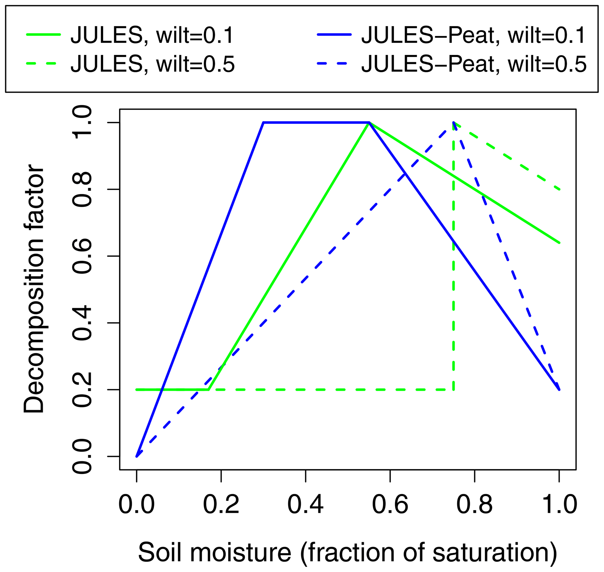
Figure 1Original (green) and updated (blue) function of moisture used to determine soil respiration (Fθ; Eq. 3).
In addition, for undecomposed organic soils specifically, critical and wilting point soil moisture can be very small due to the large pore spaces and thus low capillary suction (the critical point can be as low as 10 % saturation). The formulation of θo, on the other hand, limits the optimum soil moisture content for respiration to a minimum of 50 % saturation, which can be up 5 × higher than the critical point. The critical point is defined by a capillary suction of 3.36 m. Moyano et al. (2013) show in their Fig. 3b that the respiration response to soil moisture reaches a maximum at around this value. They show a moisture response curve for a high carbon soil in their Fig. 3a. The curve reaches a maximum at around 30 %–40 % saturation and stays at a high value until ∼ 75 % saturation, in contrast to the original formulation in JULES, which reaches its maximum only at the point θo. Therefore, for soil layers in which the critical soil moisture is lower than θo, we set the soil respiration to reach its maximum at the critical soil moisture content and remain at its maximum value until the original maximum θo, resembling the “high C content” curve in Moyano et al. (2013, Fig. 3a). We therefore define a “lower” θo, . The old and new functions are shown in Fig. 1.
The new function used in JULES-Peat is therefore
In the standard version of JULES, in situations where nitrogen is limiting, the decomposition of the litter carbon pools (decomposable plant material, DPM; and resistant plant material, RPM) is reduced. This is because the more decomposed pools have a higher nitrogen content – or lower C : N ratio – and therefore to decompose the litter carbon into the BIO (biomass) and HUM (hummus) pools requires a source of nitrogen – and nitrogen is thus “immobilised”. Thus, the decomposition terms Rpot for DPM and RPM pools are multiplied by a factor FN, which is given by
where Nin is the total soil inorganic N pool in kg [N] m−2, Mp and Ip are mineralisation and immobilisation of nitrogen, respectively, from pool p in kg [N] m−2 s−1, and Δt is the time step. DDPM and DRPM are the net demand associated with decomposition of each of the litter pools:
where p is either RPM or DPM; see Wiltshire et al. (2021) for details.
However, in reality the microbes would continue decomposing the litter pools in order to access the nitrogen for their own survival. They would not be able to transform all of the decomposed carbon into biomass due to lack of nitrogen, but the carbon would decompose and would simply be released to the atmosphere as carbon dioxide, i.e. their carbon use efficiency reduces (Manzoni et al., 2012). Therefore, instead of modifying the litter decomposition rate with the factor FN, we modify the fraction of decomposed carbon that is released to the atmosphere vs. stored in the soil. This means that the limitation term has to take a slightly different form. The new function is as follows:
The fraction of decomposed carbon that stays in the soil (rather than being released to the atmosphere), in other words the carbon use efficiency, is then multiplied by FN for the DPM and RPM pools. While nitrogen was not a focus of this study, the need for this modification became apparent once the soil column was allowed to expand with addition of plant litter. This led to an unrealistic positive feedback in which litter carbon was not decomposed due to lack of nitrogen availability, meaning that as litter was added to the layer it took up an ever larger volume, eventually pushing the more nitrogen-rich pools out of the layer completely (further down the column), resulting in zero nitrogen availability and forming unrealistically thick litter layers with no turnover.
2.3 Change of soil column height
Chadburn et al. (2017) showed that the typical soil profile simulated by ESM land surface schemes with vertically resolved soil carbon (JULES and ORCHIDEE) displays a smooth decline with depth that resembles a mineral soil profile. However, in highly organic soils the soil carbon concentration typically increases with depth to a certain point before beginning to decline (Harden et al., 2012). This is because the density of the organic material in the surface is usually lower than in the deeper soil, so there is simply less material altogether in the surface layers, and therefore less carbon. The organic material in deeper layers has a higher density: in part because it becomes compressed by soil/water above it, and in a large part because it is generally more decomposed.
The crucial missing factor in global models (e.g. JULES, ORCHIDEE, CLM) is that the models do not account for the volume that is added to the soil when organic material is added via plant litter, or (conversely) the reduction in volume when organic material decomposes. This means that as well as being unable to simulate the typical profile of a peatland (soil carbon increasing with depth near the surface), unrealistically high carbon contents in surface layers are often simulated; see the original JULES version, shown as red lines in Fig. 5.

Figure 2Functions used in JULES-Peat. Vertical dashed lines show the range of data that were used to fit the functions. These correspond to the minimum and maximum bulk densities for organic material that we derived for use in JULES (ρdpmrpm and ρbiohum; Sect. 2.3). The additional literature data for saturated hydraulic suction and the Clapp–Hornberger exponent shown in purple were derived from the following papers: Londra (2010), Rezanezhad et al. (2012), Da Silva et al. (1993), Weiss et al. (1998), Päivänen (1973), Boelter (1964), Rydén et al. (1980) and Schwärzel et al. (2006).
In JULES-Peat, the profile of litter inputs into each soil layer and decomposition of soil carbon in the layer is calculated as in Burke et al. (2017a), except that the modified decomposition function is used (Sect. 2.2). When these increments come to be applied to the soil carbon profile, however, the thickness of the soil layers is now recalculated based on the volume of organic matter added or removed. We calculate the change in layer thickness by prescribing a density to each carbon pool, using a higher density for the decomposed carbon pools than the litter carbon pools. After addition or removal of carbon in a given time step, the new effective thickness dzeff,n of soil layer n relative to the initial layer thickness dzn is given by
where ρdpmrpm and ρbiohum are the bulk densities associated with the carbon pools (in kg m−3), fc is the fraction of organic material that is carbon and dCi,n is the increment in carbon pool i in soil layer n. We picked the density of the litter pools, ρdpmrpm, to be the lowest density that is typically measured for peat (where DPM and RPM are the two litter carbon pools in JULES), and the density of the more decomposed carbon pools (ρbiohum) to be the highest density that is typically observed for peat (where BIO and HUM are the more decomposed carbon pools in JULES). Thus, the bulk density of organic material in any given soil layer will fall somewhere between these two extreme values given that each layer typically contains all four carbon pools (albeit in different ratios). The values we chose were 35 kg m−3 as the minimum, ρdpmrpm, and 210 kg m−3 as the maximum, ρbiohum. These match well with commonly quoted literature values (e.g. Chambers et al., 2010) and were derived from the 5th and 95th percentiles of the bulk densities in the global peat core dataset described in Sect. 3. These limits are shown by vertical dashed lines in Fig. 2. The maximum bulk density of 210 kg m−3 corresponds well to the threshold bulk density for peat functioning in, e.g. Wang et al. (2021). We relate the bulk density of the organic material to the carbon content by assuming that fc=0.56 or, in other words, that 56 % of the organic matter is carbon, which was also based on the 95th percentile of the percentage of carbon in the peat core dataset from Gallego-Sala et al. (2018) (see Sect. 3) and is consistent with the range of observations, e.g. in Chambers et al. (2010).
The new layer thicknesses are labelled as “effective” layer thicknesses (dzeff). In order to avoid technical difficulties and potential numerical problems with variable soil layer thickness (e.g. if surface layers become very thick), the soil carbon profile is then interpolated back onto the original soil layers.
In order to interpolate the carbon profile, the carbon quantities (C+dC; kg m−2) are first transformed to carbon densities (Cden, in kg m−3) by dividing them by the layer thicknesses, dz.
Following this, the interpolation of the effective carbon density on the effective layers back into the original layers depends on whether the centre of the original layer is above or below the centre of the effective layer and is calculated as follows:
when the original soil layer depth zn is deeper than the effective soil layer depth zeff,n, and
when the original soil layer depth zn is shallower than the effective soil layer depth zeff,n, where z is the centre of each soil layer and i indicates the carbon pool (DPM, RPM, BIO or HUM).
Mathematically, this represents an approximated second-order Taylor expansion of the function Cdens(z) around the point zeff but with a particular choice regarding the second-order derivative. In order to preserve the vertical structure of the soil, the second-order derivative is assumed to be around z+δz and z−δz, and thus if the gradient of the function changes sharply it will not be smoothed out. This means that a peat layer will not end up being numerically smeared into the rest of the profile. This is explained in detail with equations in the Supplement. Briefly, we used a simple test model where soil carbon inputs and outputs are given prescribed input and turnover rates, we account for the expansion and contraction of the soil column when carbon is added or removed and tested the method of interpolating back onto the original soil layers (i.e. as used in JULES). We ran this simple (and thus much quicker to run) script with very high resolution soil layers to see what the “true” solution for the soil carbon profile would be. We therefore confirmed that our choice of second-order derivative gave the best approximation of the true solution when a lower-resolution soil was used. For details, see the Supplement. Figure S2 in the Supplement shows that in the chosen scheme there does still appear to be some “smearing” in the deeper layers, which are thicker, but using a smaller interval δz′ leads to numerical instability in the thinner surface layers. Thus, for future development a scheme where δz′ depends on the soil layer thickness could be considered.
While the carbon profile is interpolated onto the original soil layers in order to keep the layer thicknesses constant, the thickness of the deepest soil layer is updated in order to track the overall change of soil column height. The minimum thickness for that layer is taken from the soil layer thicknesses specified at runtime, and this corresponds to the layer thickness when there is no carbon in the soil. This base layer is extended based on the total volume of the carbon pools in the soil column, and this extension is considered to be the surface elevation. However, the extra thickness of the bottom layer is neglected when calculating fluxes of heat and water and only applies when calculating carbon and nitrogen stocks and fluxes (which are conserved during layer adjustments). We decided that the complexity of modifying the heat and water calculations to account for the variable-thickness base layer was not worth the added complexity, given that the fluxes at the base of the soil column (8 m depth in this study) are generally very small.
2.4 Simulating the age profile
Peat age was simulated following a similar method to Burke et al. (2017a), where the fraction of old carbon is traced throughout the simulation. During each update of the soil carbon pools, the age of each carbon pool is tracked and the weighted average of the soil age is taken for each carbon pool in each soil layer.
Each soil carbon pool in each soil layer is assigned an age, A, at the start of the simulation, which currently is either zero on initialising the spin-up or can be initialised from an existing simulation. Each time the carbon pools are updated, the age of each soil carbon pool in each layer is increased by the time step length. These values are then modified as the soil carbon pools are updated, either due to input of fresh carbon from litter (which has an age of zero and therefore reduces the age of the soil pool), due to mixing of carbon between two layers in which the ages are different, or due to input of carbon into BIO and HUM pools from other pools via decomposition. The general formula to update the age (A) for carbon pool Ci (kg m−2), with an increment of carbon , is as follows:
ΔCi includes both incoming and outgoing fluxes from the pool. For the outgoing fluxes in ΔCi, we assume that A is the same as for the Ci pool. For an incoming litter flux we assume that A is zero, and incoming fluxes from other pools naturally take the age value from the corresponding pool.
If the soil height accumulation is switched on, the age then must be interpolated back onto the original soil layers as described in Sect. 2.3. We use the same interpolation method as for the soil carbon, which is given in Eqs. (8) and (9).
2.5 Coupling between properties and C concentration
In order to dynamically update the soil physical characteristics, we assume that the physical properties of the organic material in the soil are a function of its bulk density. The bulk density that we simulate in JULES-Peat depends on how decomposed the soil carbon is. More highly decomposed organic matter has a higher bulk density, and its properties change as it decomposes. Notably, the hydraulic conductivity becomes much lower as bulk density (or decomposition) increases, which is included in other peat models (Frolking et al., 2010; Young et al., 2017), but we also fitted relationships between the bulk density and other key physical characteristics, namely porosity, saturated hydraulic suction, the Clapp–Hornberger exponent and thermal conductivity. For the heat capacity we assumed that the heat capacity of the organic material does not significantly change with decomposition status, and therefore we used (1 − porosity, i.e. what fraction of the organic material is solids) multiplied by the heat capacity value of solids of 2.5×10⁶ J K−1 m−3, which we took from Beringer et al. (2001).
Since different carbon pools have different bulk densities (see Sect. 2.3), we first calculate the bulk density of the combined organic material in each soil layer, i.e.
where forg,n is the volumetric fraction of organic matter in the soil layer given by
Recent studies have shown that bulk density of peat shows strong relationships with its thermal and hydraulic properties (Liu and Lennartz, 2019; O'Connor et al., 2020). We combined data from these recent syntheses with additional values from the literature in order to get the best estimate of the relationships, which we show in Fig. 2. We fitted the relationships between bulk density and the other physical characteristics of peat using this combined dataset. Fitting was done using orthogonal least squares after normalising the data so that both variables being fitted had the same range of values. For the saturated hydraulic conductivity, the two available datasets showed markedly different relationships (see Fig. 2b), and thus we did not combine these but instead used only the data from Liu and Lennartz (2019) since this was a global synthesis as opposed to the O'Connor et al. (2020) data which were from a single region. The data in Liu and Lennartz (2019) also agreed better with other data, such as Wang et al. (2021), and the original values used for organic soils in JULES, originally given in Dankers et al. (2011) (also shown in Fig. 2). In addition, the fit for porosity was forced to pass through 1 at a bulk density of zero as a physical constraint (this was achieved by modifying the normalisation factor until the intercept of the fit was exactly 1). The additional literature data for saturated hydraulic suction and the Clapp–Hornberger exponent shown in purple in Fig. 2 were derived from the following papers: Londra (2010), Rezanezhad et al. (2012), Da Silva et al. (1993), Weiss et al. (1998), Päivänen (1973), Boelter (1964), Rydén et al. (1980) and Schwärzel et al. (2006).
Specifically, we relate the following soil properties to bulk density:
where Ψsat,org is soil matric suction at saturation (m), borg is the Clapp–Hornberger exponent (unitless), Ksat,org is hydraulic conductivity (in units of m s−1; note that JULES uses kg m−2 s−1 so this is multiplied by 1000 for use in JULES), θsat,org is the volumetric soil moisture at saturation (m3 m−3), λorg is the dry thermal conductivity (W m−1 K−1) and hcaporg is the dry heat capacity (J m−3 K−1). If a soil layer is not 100 % organic then we combine these calculated organic parameters with the properties of the underlying mineral soil, following Chadburn et al. (2015a). The remaining hydraulic parameters θwilt and θcrit, which are the volumetric soil moisture at the wilting point and critical point, respectively (defined in terms of hydraulic suction), are functions of the other parameters and are recalculated when the other parameters are updated (see, e.g. Chadburn et al., 2015a).
We used a large suite of simulations at 24 sites that have been use for JULES development and evaluation in Chadburn et al. (2017, 2020), Nakhavali et al. (2018), Smith et al. (2021) and Gao et al. (2022), along with Scotty Creek (Helbig et al., 2016, 2017a, b), Pleistocene Park (Euskirchen et al., 2017b), Imnavait (Euskirchen et al., 2017a), and Eight Mile Lake (Celis et al., 2019). We were able to include the four new sites that have not been used in previous studies with JULES due to additional data becoming available. The sites are fairly evenly distributed between tundra, boreal and temperate climate zones; see Table 1. Some of the sites, namely Abisko, Seida and Imnavait, provided data from different landscape types, resulting in 29 simulations in total. The climate forcing data were prepared as described in Chadburn et al. (2017) using WFD and WFDEI (Weedon et al., 2011, 2014) corrected with local climate data from the sites and covers the period 1901–2018 inclusive. The simulations were spun up for 10 000 years using repeated climate forcing data from 1901–1910.
Jammet et al. (2017)Chadburn et al. (2017)Jammet et al. (2017)Chadburn et al. (2020)Drewer et al. (2010)Gao et al. (2022)Gielen et al. (2010, 2011)Nakhavali et al. (2018)Long et al. (2010)Flanagan and Syed (2011)Gao et al. (2022)Walmsley et al. (2011)Nakhavali et al. (2018)Kittler et al. (2017)Göckede et al. (2019)Chadburn et al. (2020)Nilsson et al. (2008)Sagerfors et al. (2008)Gao et al. (2022)Celis et al. (2019)Kutsch et al. (2010)Schrumpf et al. (2011)Nakhavali et al. (2018)Euskirchen et al. (2017a)Kjellman et al. (2018)Smith et al. (2021)Fortuniak et al. (2021)Gao et al. (2022)Van der Molen et al. (2007)Parmentier et al. (2011)Chadburn et al. (2017)Aurela et al. (2009)Lohila et al. (2010)Chadburn et al. (2020)Moore et al. (2011)Brown et al. (2014)Gao et al. (2022)Euskirchen et al. (2017b)Boike et al. (2019)Chadburn et al. (2015a)Helbig et al. (2016, 2017a, b)Marushchak et al. (2013)Biasi et al. (2014)Chadburn et al. (2020)Zhang et al. (2020)Gao et al. (2022)Boike et al. (2018)Chadburn et al. (2017)Peichl and Arain (2006)Peichl et al. (2010)Nakhavali et al. (2018)Valach et al. (2021)Miller et al. (2008)Miller and Fujii (2010)Chadburn et al. (2020)Elberling et al. (2008)Chadburn et al. (2017)Table 1Sites used in the suite of JULES simulations. References are both for site data and for simulations of these sites with JULES.

Table 2JULES simulations conducted. Note that T means “true” (or the process is switched on) and F means “false” (process switched off). F → T mean that the process was switched off during spin-up and on during the main run. The “Decomp. function” refers to changing from the original to the new decomposition function shown in Fig. 1, and we also changed a switch that was using the total soil moisture instead of the unfrozen soil moisture, and thus the new decomposition function is a function of the unfrozen soil moisture (which is more realistic since frozen water is not available for microbes to use). Where the Initial C is given as “Peat”, we initialise all spin-ups with the spun up profile for Auchencorth from JULES-Peat-W, with ∼ 1.5 m of peat, and otherwise initialise the model with zero soil carbon.
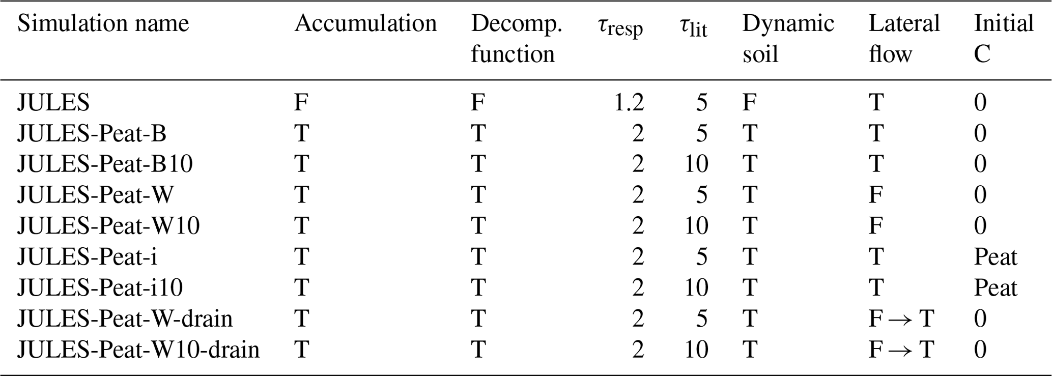
The initial JULES simulation (JULES, Table 2) is based on the configuration in Chadburn et al. (2020) but now has 20 soil layers extending to around 7.9 m, with thicknesses given in Table S3. This was originally derived from the JULES-ES configuration (see https://jules.jchmr.org/content/core-configurations, last access: 16 July 2021), with extra processes added to enhance the simulation, particularly for high latitudes. For example, an extra plant functional type (PFT) is included to represent Arctic grass, based on C3 grass with temperature optimum adjusted to grow in colder climates, layered soil carbon and nitrogen are simulated, and a bedrock column is included below the soil to simulate heat conduction. Starting from this baseline simulation, we then activated the new processes in JULES-Peat described in Sect. 2. See the Code and Data Availability section for the full configuration.
For most of the simulations the standard TOPMODEL-based large-scale hydrology scheme was used, which calculates the lateral flow of water from each grid cell based on the topographic index information of the grid cell (Gedney and Cox, 2003). In order to simulate a wetter site, for example a topographically controlled peatland, which would essentially be a wetter fraction of the grid cell than the grid cell average, we simply set the lateral flow to zero (JULES-Peat-W and JULES-Peat-W10, Table 2). Neither of these hydrological scenarios are necessarily expected to be realistic for the sites. The aim was to test the response of the model to wetter vs. drier conditions. How to simulate peatland hydrology realistically is a challenge and will be addressed in future work (see also Bechtold et al., 2019). In JULES-Peat-W-drain and JULES-Peat-W10-drain (Table 2), the lateral flow is set to zero during spin-up but switched back on during the main run to approximate drainage.
The list of simulations is shown in Table 2. JULES-Peat-B and JULES-Peat-B10 are baseline JULES-Peat simulations. The impact of switching off the lateral flow (JULES-Peat-W and JULES-Peat-W10) and initialising the sites with peat (JULES-Peat-i and JULES-Peat-i10) – instead of letting the carbon build up from zero – was then tested. Initialising with peat soil tests whether the model retains a peat layer at sites where peat was not able to form from scratch, which would indicate self-regulating functions of peat in JULES-Peat. To initialise with peat we used the spun-up profile from Auchencorth JULES-Peat-W simulation, since this simulation had formed a thick, 1.7 m layer of peat (see Fig. S12). The only site that formed thicker peat in JULES-Peat was CA_WP1, which formed an extremely thick (5–6 m) peat layer (Table S4, Fig. S12), and thus we chose Auchencorth as a site with a thick but not extreme peat profile. In addition to these simulations, new processes were firstly switched on one by one in factorial until the full “JULES-Peat” was run – these simulations are shown in the Supplement. During this process a few different parameter combinations were tested to make sure the soil carbon profile and the age–depth profile looked realistic. In particular we altered the rate of decay of soil respiration with depth (efolding), τresp, and the efolding depth of litter inputs to the soil, τlit (called ξlit in Wiltshire et al., 2021). A higher value of τlit means more of the litter is added to the surface compared to deeper in the soil. We ran JULES-Peat with two different values of τlit, 5 and 10, where 5 is the original value in JULES and any simulation with a “10” on the end (Table 2) has τlit=10. Note that we did not develop the vegetation module further here, and this should be addressed in future work (Sect. 5.3).
For evaluation we used a globally distributed dataset of peat profiles (Gallego-Sala et al., 2018). We divided these data into major climate zones and selected only those zones that are covered by the JULES simulations: temperate, boreal and tundra. This left 216 sites: 12 tundra, 127 boreal and 77 temperate. We compared these peat profiles against the site simulations divided into the same climate zones. We also used this dataset to derive the values for maximum and minimum bulk density (ρdpmrpm and ρbiohum; see Sect. 2.3) and the fraction of carbon in organic matter (fc). For this calculation we selected only the data points that were organic rich with minimal mineral content, for which the percentage of carbon (by mass) was higher than 30 %. This left over 24 500 data points where the vast majority of the soil by volume is organic material.
Before comparing the peat core dataset against the JULES simulations, we only remove values where the percent carbon is less than 15 % as we take this as a common definition of organic soil (United States Department of Agriculture, 1975), which can include some mineral material. We use the same definition to assess where JULES-Peat simulates a peat or a mineral soil, noting that to estimate the percent carbon by mass in JULES, we assume the mineral fraction of the soil has a bulk density of 1500 kg m−3 (Hossain et al., 2015). We isolate the peat layers from the JULES simulations in order to evaluate comparable soil layers against the observed peat core dataset and select only sites where JULES simulates peat in at least the top four soil layers (i.e. to 39 cm depth, since this is the closest layer to the 40 cm depth specified for defining organic soils; United States Department of Agriculture, 1975).
For further evaluation data we used individual soil carbon profiles from other data sources, which are available for some of the sites in Table 1 (references given in the table).
4.1 Representation of mineral soils
Since JULES is a global model, it is important that adding the functionality to represent peat does not degrade model performance for mineral soils. Therefore, we first evaluate the model at mineral soil sites.
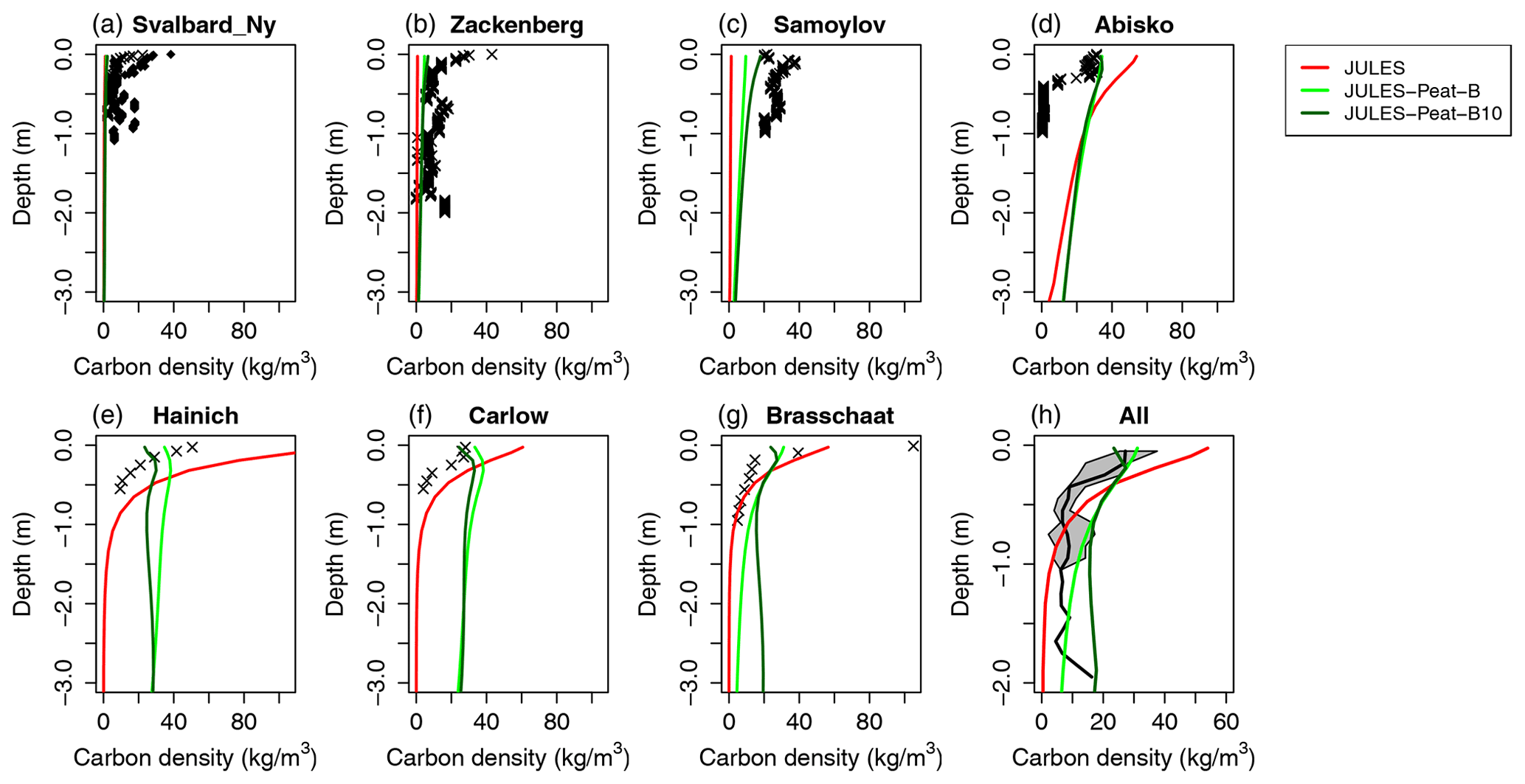
Figure 3Evaluation at mineral sites. Observations are shown with black crosses or lines. The black line in (h) is the median of all sites, with the grey area indicating the interquartile range. Note that the axis ranges are different in (h). The simulations JULES-Peat-B and JULES-Peat-B10 have different values of τlit. For information about the sites refer to Table 1, and for details of the JULES simulations refer to Table 2.
In soils where the organic material is a relatively small fraction of the total soil, the original soil carbon scheme is able to perform well, since the expansion of the soil column due to the addition of organic material will be relatively small. Figure 3 shows the model performance at mineral soil sites where measured soil carbon profiles were available. While the individual sites are not well simulated, the general form of the profiles – resembling an exponential decline with depth – are recreated reasonably well in the standard JULES configuration.
Table 3RMSEs of JULES simulations against various observations. “Temp.” is short for temperate. The final two columns refer to the median of the site-specific observations shown in Figs. 3 and 4 respectively. The best-performing simulation for each column is highlighted in bold.
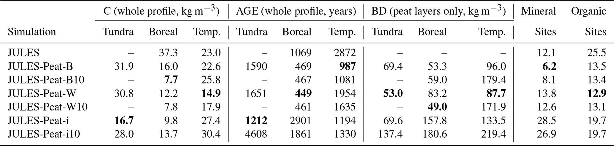
Figure 3 also shows two JULES-Peat simulations in light green and dark green (JULES-Peat-B and JULES-Peat-B10, respectively, Table 2). As discussed in Sect. 3, these have different values of τlit and are both plausible. In general, the new model version is also able to simulate a profile that resembles a mineral soil despite forming peaty profiles at a few of the sites, especially Hainich and Carlow (where the carbon is overestimated by all configurations of JULES, Fig. 3e–f). Aggregated across all sites, the updated model versions produce a profile with somewhat lower carbon density at the surface compared to standard JULES and less of a decline in carbon with depth (Fig. 3h). The lower carbon density at the surface matches better with observations than the original JULES simulation, but the carbon at depth tends to be overestimated. In terms of root-mean-squared error (RMSE), the aggregated profile is improved in JULES-Peat-B and JULES-Peat-B10 (RMSE 6.2 and 8.1 kg m−3) compared to JULES (RMSE 12.1 kg m−3); Table 3. Overall we conclude that despite poor model performance at individual sites, the aggregated soil carbon profiles in both JULES and JULES-Peat adequately resemble observed mineral soil profiles (Fig. 3h).
4.2 Model evaluation at peatland sites
We assess the performance of the full JULES-Peat model configuration at the selection of simulated sites for which observed soil carbon profiles are available and organic soils are present (Fig. 4). A few of the individual sites are well simulated, and almost all sites are simulated significantly better in all of the JULES-Peat configurations than they are in JULES (RMSE of median profile 12.9–13.5 kg m−3 for JULES-Peat configurations shown and 25.5 kg m−3 for JULES; Table 3). Note that two additional JULES-Peat simulations are shown in Fig. 4, JULES-Peat-W and JULES-Peat-W10 (dark blue and light blue lines, respectively), where the lateral water flow is set to zero since we expect that this would lead to a wetter soil and a more realistic simulation of a topographically controlled peatland.
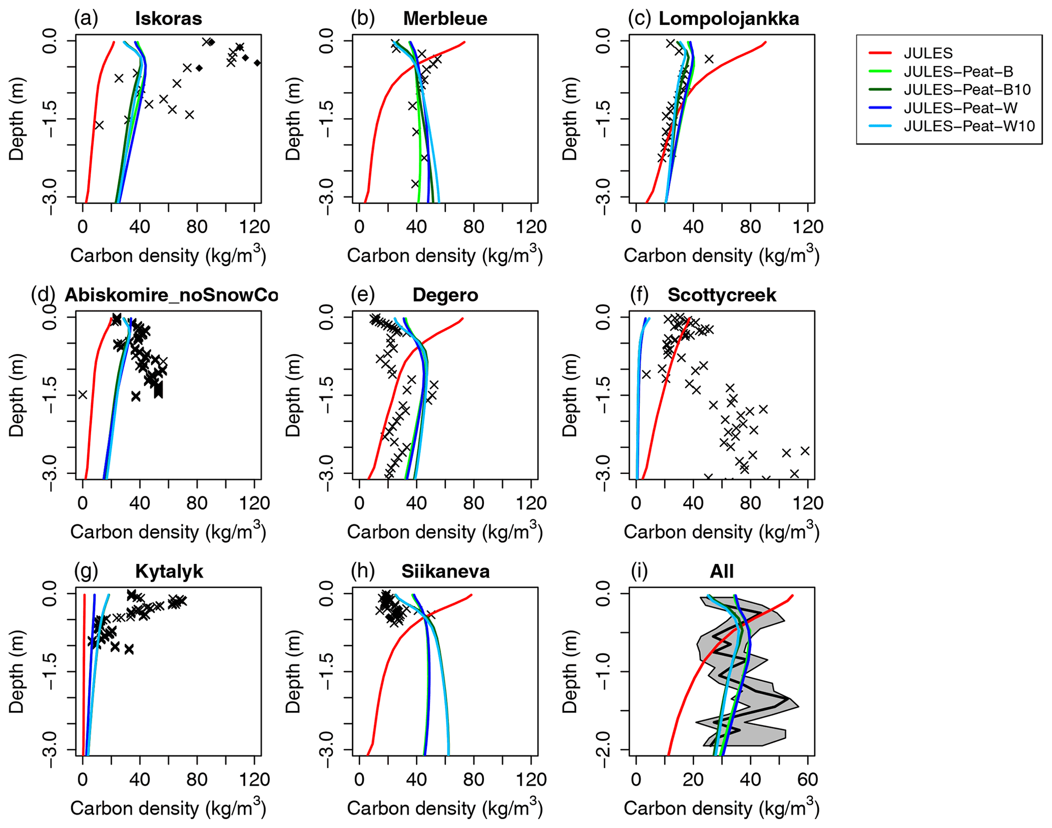
Figure 4Evaluation at organic sites. Observations are shown with black crosses or lines. The black line in (i) is the median of all sites, with the grey area indicating the interquartile range. Note that the axis ranges are different in (i). In JULES-Peat-W and JULES-PeatW10 (dark blue and light blue lines, respectively) the lateral water flow is set to zero. The simulations with “10” on the end have τlit=10. For information about the sites refer to Table 1, and for details of the JULES simulations refer to Table 2.

Figure 5Evaluation of JULES-Peat carbon profile against the median profile from peat cores. The grey-shaded area shows the interquartile range. Only sites where the model simulates a sufficiently thick organic layer to classify it as peat (> 15 % carbon by mass for ≥ 39 cm; see Sect. 3) are shown. The sites that are shown for each simulation are highlighted in bold in Table S4.
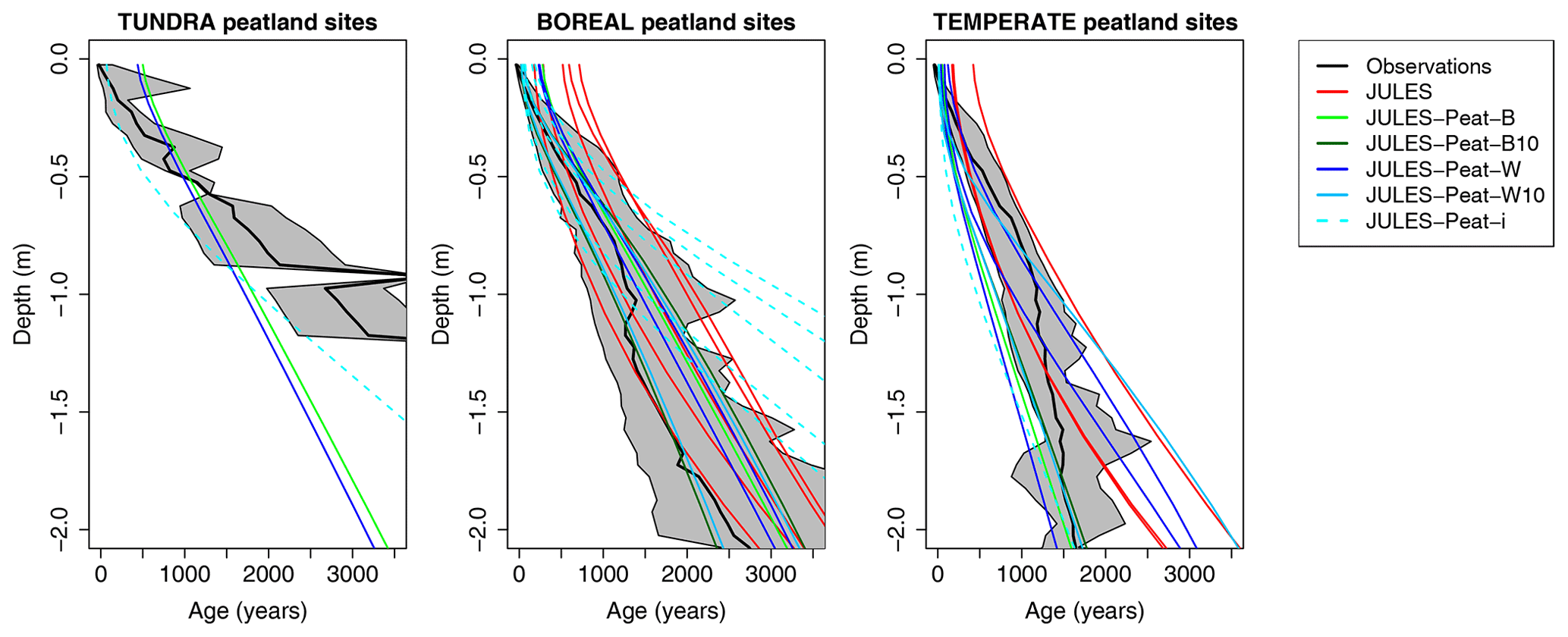
Figure 6Evaluation of JULES-Peat age–depth profile against the median profile from peat cores. The grey-shaded area shows the interquartile range. Only sites where the model simulates a sufficiently thick organic layer to classify it as peat (> 15 % carbon by mass for ≥ 39 cm, see Sect. 3) are shown. The sites that are shown for each simulation are highlighted in bold in Table S4.
We then evaluate the soil carbon and age–depth profiles in JULES and JULES-Peat against the global dataset of peat cores (described in Sect. 3) (Gallego-Sala et al., 2018) in Figs. 5 and 6. These figures show simulated soil carbon profiles at sites where the model simulates a carbon percentage by mass of more than 15 % for at least 39 cm (see Sect. 3) and compares these against the median of the equivalent data (percent carbon > 15 %) from the global dataset of peat cores (Gallego-Sala et al., 2018). It is clear that at these peaty sites, the original JULES configuration simulates a carbon density that is too high in the surface layers and too low in the deeper soil (red lines in Fig. 5).
In order to quantify the total improvement in the various JULES-Peat simulations compared with the original JULES configuration we take the RMSE between the median soil carbon profiles for each climate zone, shown in Table 3. The best-performing version (shown in bold) has a RMSE that is reduced by 35 % for temperate peatland sites (from 23.0 to 14.9 kg m−3, Table 3) and by almost 80 % for boreal peatland sites (RMSE reducing from 37.3 to 7.7 kg m−3, Table 3). We see that the age at the soil surface was typically too high in the original configuration of JULES (Fig. 6, red lines). In JULES-Peat, the age at the soil surface is better simulated, age throughout the profile is generally realistic (solid blue and green lines in Fig. 6, mostly falling within the interquartile range of the observations), and RMSE in age is reduced by 32 % (temperate sites) and 56 % (boreal sites) for the configurations that perform best in terms of carbon profile (JULES-Peat-W and JULES-Peat-B10 respectively, Table 3).
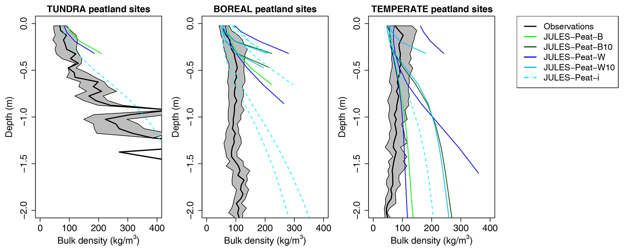
Figure 7Evaluation of JULES-Peat bulk density profile against median profile from peat cores. The grey-shaded area shows the interquartile range. Only sites where the model simulates a sufficiently thick organic layer to classify it as peat (> 15 % carbon by mass for ≥ 39 cm, see Sect. 3) are shown. The sites that are shown for each simulation are highlighted in bold in Table S4. Model profiles are cut off because only the organic layers are plotted.
We also evaluated the bulk density profiles against the same peat core dataset, and the results are shown in Fig. 7. The bulk density in JULES-Peat tends to start at realistic values at the surface but increases too quickly with depth. It is remarkable how little the observed bulk density at boreal and temperate peatland sites varies with depth compared with the tundra sites (Fig. 7), although this may be related to the larger sample size of boreal and temperate sites (127 and 77 vs. 12 for tundra) leading to a more “smoothed” profile.
4.3 Impact of environmental and initial conditions on peat profiles
The best simulations in JULES-Peat are generally those where drainage is impeded to make the soil wetter (JULES-Peat-W; see the bold numbers in Table 2). In particular, JULES-Peat-W simulates a more realistic carbon density profile than the other model configurations for the temperate peatland sites (see the dark blue lines in Fig. 5). For the boreal sites, JULES-Peat-W10 accurately captures the gradient of the soil carbon profile in the top 50 cm of soil (light blue lines in Fig. 5). The age–depth profiles in JULES-Peat-W and JULES-Peat-W10 also correspond most closely to the median measured age–depth profiles. Since peat generally forms in wetter places, the fact that the simulations without lateral water flow out of the soil (JULES-Peat-W and JULES-Peat-W10) compare best against observations from peat soils is expected if the model realistically forms more peat in wetter soils.
In simulations whose name ends with “10” (e.g. JULES-Peat-W10, shown in light blue) the distribution of litter inputs into the soil is more weighted towards the surface (τlit=10 as opposed to 5, Table 2). We generally find that using the lower value of τlit matches better with the data for the temperate peatlands and that the higher value is better for boreal peatlands (see the RMSE values for carbon profile in Table 3). This suggests that τlit should depend on plant functional type, which it would in reality (shallower-rooting plants would deposit more of their litter nearer the surface) and implies that smaller or shallower-rooting PFTs should grow in colder regions, as is indeed the case (Jackson et al., 1996).
JULES-Peat was sometimes able to accumulate peat starting with no carbon in the soil at time = 0 at one of the tundra sites (Iskoras) in selected configurations (JULES-Peat-B and JULES-Peat-W, see Fig. S12). These simulations form a relatively thin organic layer at this site. However, when the simulations were initiated with an existing peat profile instead of zero soil carbon in JULES-Peat-i (see Table 2), the peat profile was maintained at Iskoras and continued to accumulate (Fig. S12 and Table S4). This then forms a realistic carbon density profile and a reasonably realistic age–depth profile, shown by dashed cyan lines in Figs. 5a and 6a. There are multiple reasons why the model may not accumulate much peat at tundra sites, including a lack of representation of more favourable paleoclimate conditions during spin-up and the simulation of soils that are too dry (Smith et al., 2021). Nonetheless, the Iskoras simulation by JULES-Peat-i indicates that when the model does simulate peat at a tundra site it can form a realistic profile (Fig. 5a, dashed cyan line). Similarly, the bulk density profile simulated for the tundra sites is realistic for the JULES-Peat-i simulation (dashed cyan line in Fig. 7).
4.4 New processes in JULES-Peat
We initially introduced the additional processes and parameter changes that were incorporated in JULES-Peat into simulations one by one to test each process before running the full model. These simulations are shown in the Supplement (Sect. S2). The key development that allows the shape of the carbon profiles to be more realistic is accounting for the volume of organic material added and removed from the soil column (Eq. 7) as described in Sect. 2.3. In particular, this process enables more carbon to reach the deeper soil and makes the carbon density in the surface lower since it expands when plant litter (which has low density; ρdpmrpm=35 kg m−3) is added. These differences are clear in all of the JULES-acc and JULES-Peat simulations in comparison to the original JULES (Figs. S3 and 5). The majority of the reduction in RMSE is already achieved by adding in this process alone (reduced from 23.0 to 10.4 kg m−3 at temperate sites and 37.3 to 17.3 kg m−3 for boreal sites; Table S2).
While it does not significantly reduce the RMSE by itself, modifying the moisture function to suppress decomposition when saturated (Sect. 2.2, Eq. 3) allows more peat to form in wetter areas, which is a crucial factor in simulating realistic peatland distribution and future dynamics. Reducing drainage makes the simulation worse for mineral soil sites, which is exactly what would be expected (wetter soil ⇒ more peat forms), and it almost universally improves carbon profiles for organic sites (compare JULES-Peat-B and JULES-Peat-B10 against JULES-Peat-W and JULES-Peat-W10 in Table 3).
The other major new process introduced is that JULES-Peat simulates its own soil characteristics (Eqs. 13–18, Sect. 2.5). While we do not have measured profiles of soil characteristics to compare against, we can compare the soil thermal and hydraulic parameters simulated by JULES-Peat against those prescribed in JULES. Comparisons are shown in the Supplement for key parameters: Ksat, Ψsat, θsat and b for the simulations JULES-Peat-B, JULES-Peat-B10 and JULES-Peat-i10 (Figs. S7–S10). For some sites there is a good correspondence between the simulated and prescribed parameters, while for others there are significant differences, but all simulated profiles behave sensibly.
Simulating these soil properties dynamically leads, in many cases, to a thicker organic layer (compare JULES-accC and JULES-accC10 with JULES-Peat-B and JULES-Peat-B10 in Table S4) and more soil organic carbon (Figs. S5 and S6). This increase in carbon results in profiles that are significantly more realistic for organic sites (Fig. S6; RMSE reduced from ∼ 18–20 to 13–14 kg m−3) and marginally less realistic for mineral soil sites (Fig. S5; RMSE increased from ∼ 6–7 to 6–8 kg m−3). This suggests a self-reinforcing feedback of peat accumulation with soil characteristics, e.g. if peat accumulation has started, it is more likely to continue, and can lead to various important dynamics, which are discussed in the following sections.
5.1 Drainage, subsidence and feedbacks between hydrology and soil carbon
For the simulations where the lateral flow of water was switched off during spin-up in order to simulate a wetter and more “peaty” soil (JULES-Peat-W and JULES-Peat-W10), we ran an alternative realisation of the 20th century where the lateral flow was switched back on (JULES-Peat-W-drain and JULES-Peat-W10-drain). At many sites the lateral flow is negligible in any case and this does not significantly affect the results. However, at some sites the “wet” (-W) simulation maintains a water table near the surface, whereas the baseline simulation (JULES-Peat-B/JULES-Peat-B10) does not, and the drained simulations therefore experience a major drop in water table and a subsequent degradation of the peat and a drop in the surface elevation (subsidence). Figure 8 shows the four sites for which the change in water table is most pronounced in JULES-Peat-W-drain (water table change given in Table 4).
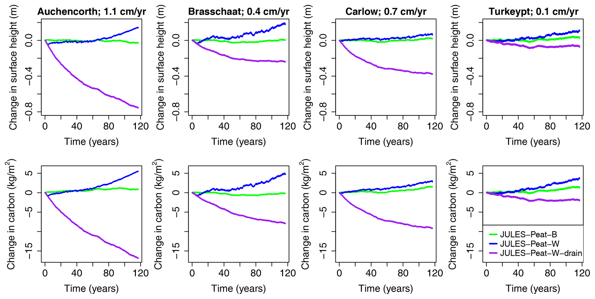
Figure 8Carbon and surface height dynamics following drainage: JULES-Peat-W and JULES-Peat-W-drain are both spun up with a wet soil column, but JULES-Peat-W-drain has lateral flows switched back on at the start of the historical simulation, which is shown here. JULES-Peat-B is also shown for comparison, showing that carbon does not accumulate at these sites to the extent that it does when the sites are wet (compare JULES-Peat-B to JULES-Peat-W). Subsidence rates (in cm yr−1) over the first 40 years are indicated in the panel labels. Water table depth in each simulation is given in Table 4.
Table 4Median water tables corresponding to the simulations shown in Fig. 8.
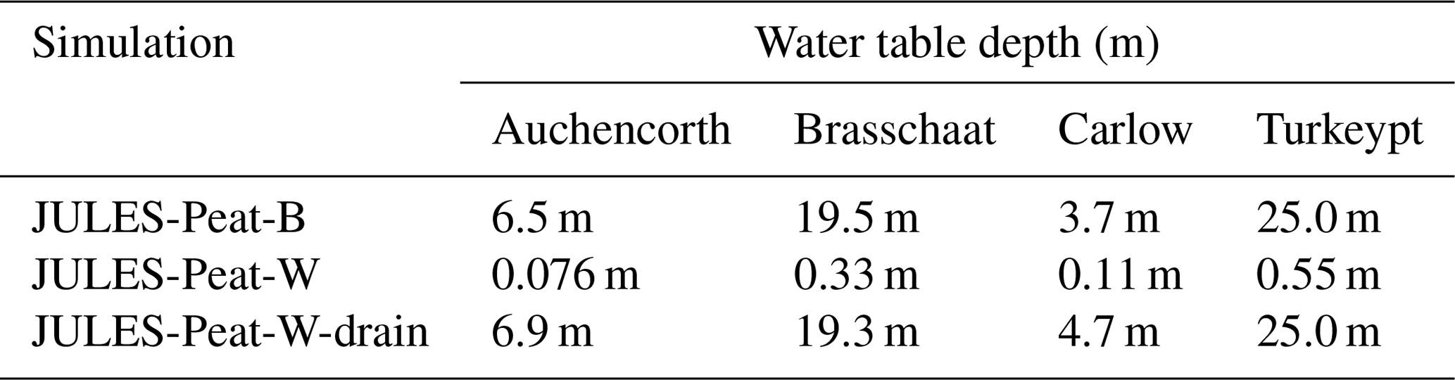
Liu et al. (2020) tracked the surface subsidence rate over time following drainage of peatlands for two different land use practices – forestry and agriculture. They typically see a very high subsidence rate of around 3–10 cm yr−1 in the first few years after drainage. Following this, a more steady subsidence rate of 0.5–2 cm yr−1 can be observed for the next few decades. In the sites in Fig. 8, we see a surface subsidence rate more in line with the longer-term subsidence rate of 0.5–2 cm yr−1 (e.g. Auchencorth loses > 40 cm in the first 40 years and 60 cm in around 80 years; see Fig. 8). The lack of the initial very rapid subsidence suggests that there may be some processes missing in JULES, for example the mechanical raising and lowering of the peat surface by as much as tens of centimetres as the water table fluctuates, known as bog breathing (Howie and Hebda, 2018). However, the long-term subsidence rate is at least of the right order of magnitude. After an initial period of subsidence lasting around 50 years, the drop in surface height stabilises or slows. The carbon loss behaves in a similar way, although the slowing of carbon loss is not as pronounced. In these test simulations (noting that the method of “draining” the sites is a proof of concept and is not based on reality), up to 17 kg C m−2 is lost from these sites, which would represent a highly significant addition of carbon to the atmosphere (on the order of tens of gigatons of carbon globally) if it took place across a significant fraction of the world's peatlands.
Both positive and negative feedbacks exist within peatland ecosystems (Waddington et al., 2015). JULES-Peat is able to capture some of the key feedbacks by simulating dynamic soil properties. Firstly, a negative (damping) feedback takes place following drainage in which the peat compacts and becomes more resistant to water flow, thus re-wetting the soil to some extent; see Fig. 9. There is a strong correlation between decreased hydraulic conductivity and increased soil moisture: Pearson correlation between soil moisture and log (Ksat) of −0.94 for Auchencorth and −0.87 for Carlow (in the top 3 m) using monthly data points for individual layers for the whole simulation. In these particular simulations, this effect was not strong enough to bring the water table back to the surface by the end of the simulation, but in some test simulations this effect was observed. In reality, it is rare for drained peatlands to self-restore, but it does occasionally happen (Alice Milner, personal communication, 2021; Morag Angus, personal communication, 2021). On the other hand, a similar mechanism can lead to a positive (amplifying) feedback during spin-up, where the accumulation of peat leads to a lower drainage rate and thus further accumulation of peat. This is seen most strongly at Auchencorth and Carlow, which are the only sites from the UK and Ireland that were simulated (Fig. 10). After sufficient peat formation (in particular after being initialised with peat in JULES-Peat-i and JULES-Peat-i10; see Table 2), these sites are able to gradually raise their water tables over the course of the spin-up, while accumulating more and more carbon; see Fig. 10. It is significant that the UK and Ireland sites are the only ones where this mechanism takes place, since this is where the majority of the world's blanket bogs are found – peatlands that are able to maintain themselves autogenically without topographic controls. This indicates that JULES-Peat should be capable of simulating blanket bogs, which are currently missing in global peatland models due to their reliance on TOPMODEL-based wetland fraction to determine peatland area (Müller and Joos, 2020).

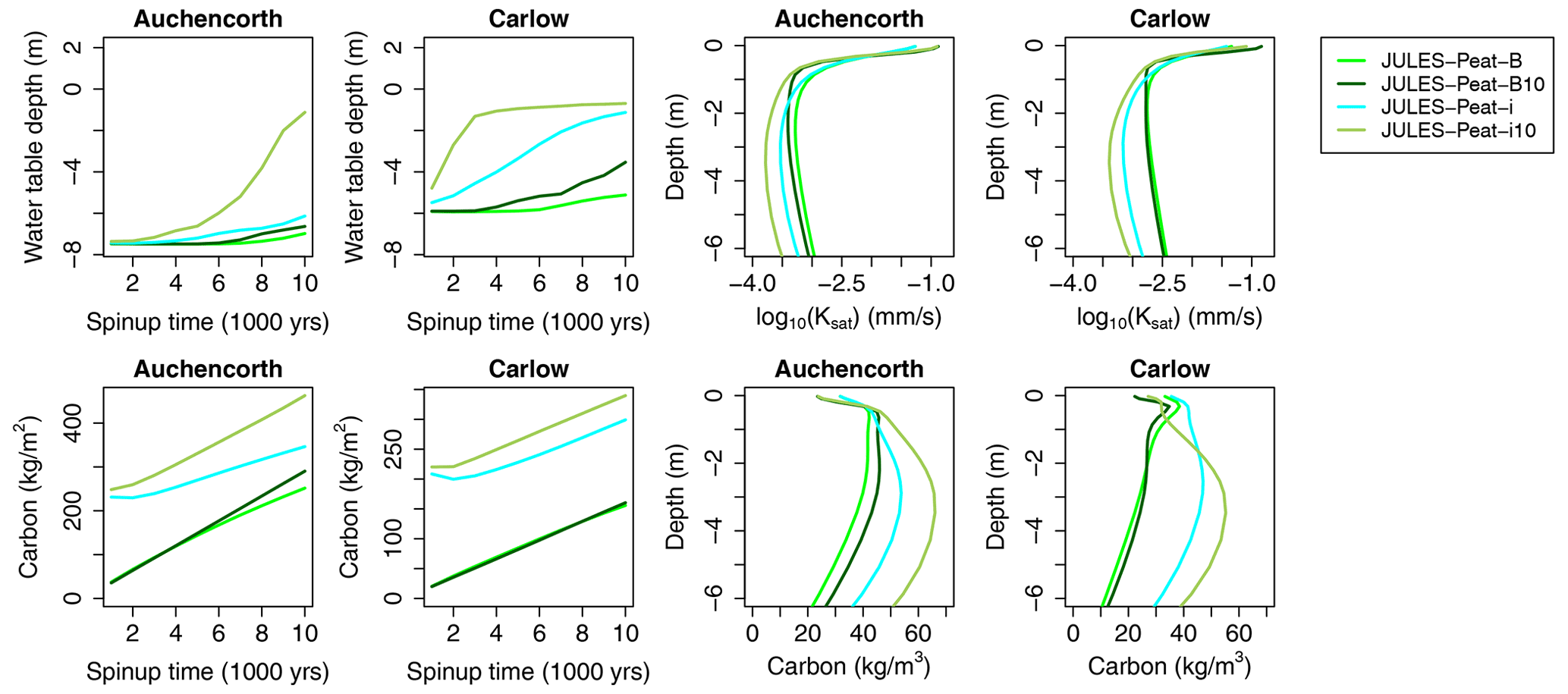
Figure 10Hydrological feedback between peat accumulation and water table level. Note that the spin-up time is noted in thousands of years so the total spin-up period is 10 000 years. Vertical profiles of Ksat and carbon are shown at the end of the spin-up.
5.2 Multiple steady states
Since there are feedbacks in JULES-Peat between soil physics and soil carbon that can be self-reinforcing, the “end state” of the model spin-up now depends on the initial conditions. In mathematical terms there can be more than one equilibrium state. This also implies the existence of tipping points where the system can “tip” from one state to another under sufficient forcing (Ritchie et al., 2021). Essentially, there may be some sites at which initialising the model with peat allows it to further accumulate peat, but initialising the model with mineral soil maintains a stable mineral soil profile. Practically, this means that peat can exist outside of climatic conditions where it would form from scratch, and thus this is very important when we consider the disturbance of existing peatlands for which the original state could be impossible to recover under current climates.
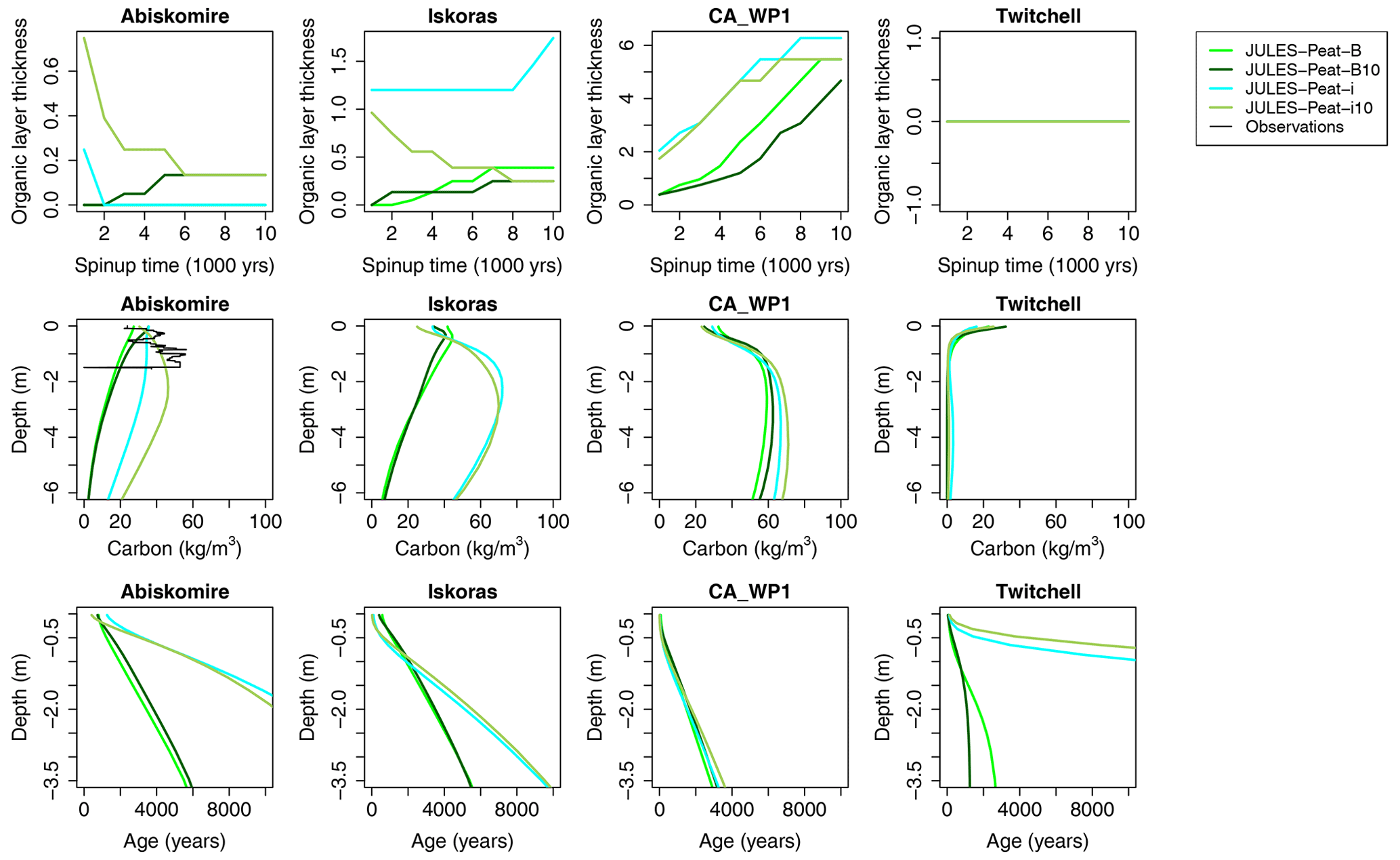
Figure 11Demonstration of how peat accumulation rate can depend on initial conditions. Profiles of carbon and age are shown at the end of spin-up. Note that the ages below a certain depth at Twitchell are not relevant due to the carbon pools being almost zero. Note also that the spin-up time is given in thousands of years (so the total spin-up period is 10 000 years).
In order to test this we compare the simulations where peat is initialised vs. not initialised in Fig. 11. We show two sites where peat only accumulates when it is initialised (Abiskomire_noSnowCor and Iskoras), a site where peat always accumulates (CA_WP1), and a site where peat never accumulates and a mineral soil always forms (Twitchell). This behaviour is apparent in the age–depth profiles (bottom row of Fig. 11). The age is initialised with the existing age–depth profile of the peat for the runs that are initialised with peat (JULES-Peat-i and JULES-Peat-i10), hence the ages overall can be higher, since the standard runs start from age zero with no carbon. However, when the model converges to a single steady state, the age profile also starts to converge, at least at the surface (Twitchell and CA_WP1 in Fig. 11). In contrast, at sites where peat only accumulates when the model is initialised with peat, the age at the surface actually becomes lower in the simulations where it was initialised with an existing age–depth profile than in the simulations where it was initialised at zero. This indicates that carbon is accumulating more quickly when the model is initialised with peat (-i and -i10) (Abiskomire_noSnowCor and Iskoras in Fig. 11).
It is interesting to note that the sites where highly distinct steady states are simulated are palsa mires in the sporadic permafrost zone. These sites are on the cusp of the permafrost–non-permafrost transition. Thawing of permafrost peatlands has been shown to increase the carbon accumulation rate in some cases (Turetsky et al., 2007), and, interestingly, the simulations with high peat accumulation rate at Abiskomire_noSnowCor and Iskoras (JULES-Peat-i and JULES-Peat-i10) simulate a thawed soil, whereas the simulations with little peat accumulation (JULES-Peat-B and JULES-Peat-B10) simulate permafrost (Fig. S11).
Table 5Dominant vegetation type and fraction at the end of the spin-up for the sites and runs shown in Fig. 11. EG stands for evergreen.
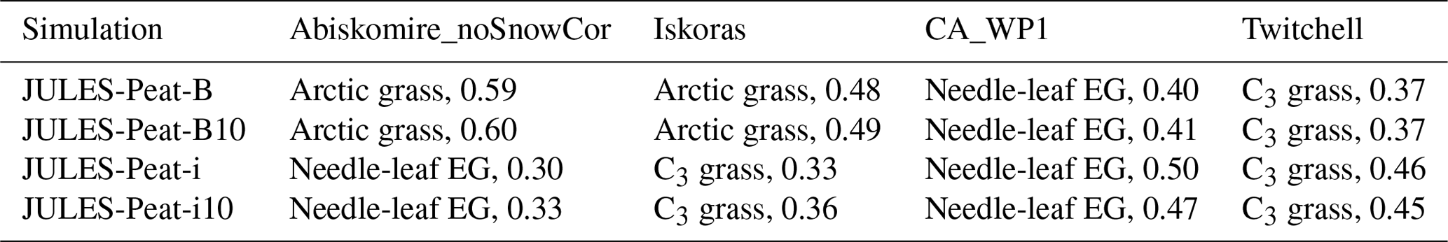
The different steady states also appear to be associated with the presence of different vegetation types; see Table 5. The sites that develop very different carbon profiles when initialised with peat (Abiskomire_noSnowCor and Iskoras, JULES-Peat-i and JULES-Peat-i10) also develop a different dominant vegetation type, for example needle-leaf evergreen trees instead of Arctic grass in Abiskomire_noSnowCor (Table 5). This interaction between vegetation and soil carbon highlights the importance of further developing the vegetation model to represent peatland vegetation (see Sect. 5.3 for further discussion). It is worth noting that for a site that simulates peat accumulation, the “steady-state” condition can be a constant rate of carbon accumulation rather than a constant quantity of carbon, i.e. peatlands are never in equilibrium, which differs from the standard definition of steady state that is currently used when spinning up land surface models.
5.3 Next steps for modelling global peatlands: hydrology and vegetation
Simulating landscape-level peatland hydrology is a major challenge. This work has taken a step forward by enabling peat soils to react appropriately to long-term changes in hydrology and to include some of the key feedbacks that the soils then have on the water flows. We have also recently developed an improved methane emissions scheme (Chadburn et al., 2020). However, to model peatlands within the landscape globally, including any methane emissions, the distribution of water around the landscape must be taken into account.
For instance, the majority of peatlands globally are topographically controlled. This means they are found in flat, lowland areas (Sheng et al., 2004; Martini, 2006). The standard way of modelling groundwater in ESMs does not explicitly model these areas but simulates a “grid cell average” soil moisture. This means that at typical resolutions, the saturated lowland areas where peat forms would be less than the size of a grid cell, and thus saturated conditions would never be explicitly simulated, and secondly, even with a high enough resolution to resolve peatlands, there is no mechanism for lowland grid cell soils to receive water from the surrounding uplands. Therefore, a key step is to explicitly model different hydrological regimes and features within the landscape. The simplest way to do this is via a tiling approach. Bechtold et al. (2019) found that they were able to recreate the hydrological dynamics in the majority of the world's peatlands by using a tile that was entirely hydrologically disconnected from the rest of the grid cell. A further step would be to simulate the hydrological connection between the tiles in the grid cell, as this is necessary to simulate not only some existing peatlands but also peatland initiation (Väliranta et al., 2017).
Furthermore, the within-soil-column hydrology is not well modelled for organic soils in JULES. While peatlands in JULES-Peat are able to maintain a water table through the hydraulic characteristics of the peat itself, the water table generally does not sit as close to the surface as the observed water table in intact peatlands, which is around 10 cm (Evans et al., 2021) (see, e.g. Carlow in Fig. 10), although it can occasionally reach 10 cm when lateral flow is set to zero (Table 4). In cold regions, a representation of ponding can be necessary to prevent too much snowmelt from running off and leaving the soil too dry (Smith et al., 2021). On top of this, the hydraulic behaviour of mosses, which form a primary component of high-latitude and temperate peatlands, is very different from that of vascular plants. Mosses do not extract water from the soil and it essentially only evaporates from the surface, which could very well lead to a raised water table (Van Breemen, 1995). Thus the inclusion of a moss PFT and its unique functions in land surface models like JULES should be a priority, and several models have indeed done this (e.g. Porada et al., 2016; Chaudhary et al., 2017; Shi et al., 2021).
It is clearly important to adequately represent the features of peatland vegetation. As well as the hydrological behaviour of mosses, it will be crucial to include an appropriate distribution of plant litter inputs to the soil (see the difference between the simulations with different values of τlit, e.g. in Fig. 5), an appropriate recalcitrant litter fraction (for example, mosses are more recalcitrant than grass and therefore more likely to lead to peat accumulation), and suppression of the growth of non-wetland vegetation such as trees under saturated conditions (this is not included in JULES and is necessary to simulate the mossy peat that is found in northern latitudes, since larger vegetation would otherwise outcompete the mosses). In addition, the input of carbon to the peat is determined by the net primary productivity of the ecosystem, and thus this is a key quantity to evaluate when developing peatland-appropriate PFTs.
Finally, the JULES-Peat model configuration has not yet been tested in tropical peatlands, which differ from northern peatlands in terms of hydrology and vegetation and have only recently gained attention in the modelling community (Kurnianto et al., 2015; Apers et al., 2021). There is a clear need for more focused study of tropical peatlands, given their large spatial extent and carbon stock and the potential impacts of their ongoing drainage (Dargie et al., 2017; Mishra et al., 2021). Some of the key principles behind peat dynamics are universal (for example, suppression of decomposition in wet soils, dynamic growth of the soil surface), but model parameters such as those in the relationships used to determine soil characteristics may need to be updated for tropical peat (e.g. Eqs. 13–18).
We have demonstrated a new scheme integrated in an ESM land surface model that can simulate both peat and mineral soils depending on site conditions and that can simulate dynamic transitions from peat to mineral soil or vice versa. The new model configuration, which we call JULES-Peat, includes some key ecohydrological feedbacks that take place in peat soils. At some sites, whether or not peat accumulates depends on the initial conditions.
The model performs well by all metrics that we compared it against, and it can now simulate a soil profile that resembles peat for the first time in JULES. As well as simulating mechanisms that determine the (in)stability and resilience of peatlands for the first time, this model has the potential to simulate blanket bogs, which current global peatland models are unable to do (Müller and Joos, 2020). We noted when designing the interpolation scheme (Sect. S1) that the interpolation can lead to some “smearing” of the carbon profile in the deeper soil, and indeed the model does not simulate sharp transitions between peat layers and underlying mineral soil that can often be seen in reality. Thus some improvement to the interpolation scheme may still be possible, which could also lead to improved physical soil characteristics. It should also be noted that the JULES soil layers need to be set at a sufficiently high resolution to be capable of resolving such a transition.
As outlined above in Sect. 5.3, major challenges remain around appropriately modelling peatland vegetation and large-scale hydrology, as well as a need to test the model for tropical peatlands. It may also be necessary to model microtopography and/or ponding in order to simulate soil hydrology correctly (Smith et al., 2021). Since models individually tackle different parts of this problem, the next steps will inevitably involve combining existing schemes, or at least concepts, for simulating vegetation, large-scale hydrology and microtopography with the soil dynamics simulated here in JULES-Peat (e.g. Bechtold et al., 2019; Porada et al., 2016; Shi et al., 2021), along with the latest methane emissions schemes (e.g. Chadburn et al., 2020).
Peatlands are of utmost importance in terms of mitigating climate change, both as carbon sinks and as potentially very large carbon sources that may exacerbate climate change (Leifeld and Menichetti, 2018). Modelling global peatlands and their dynamics should therefore be a priority for land surface and Earth system modelling.
Both the model code and the files for running it are available from the Met Office Science Repository Service: https://code.metoffice.gov.uk/ (last access: 8 February 2022). Registration is required, and code is freely available subject to completion of a software license. The results presented in this paper were obtained from running the following JULES branch: https://code.metoffice.gov.uk/trac/jules/browser/main/branches/dev/sarahchadburn/vn5.8_accumulate_soil, version 20669 (last access: 16 July 2021, Chadburn and JULES collaboration, 2021, registration required), which is a branch of JULESv5.8 with the new code described in this paper added to it. The runs were completed with the Rose suite: https://code.metoffice.gov.uk/trac/roses-u/browser/c/g/3/6/5/, version 200810 (last access: 16 July 2021, Burke et al., 2021, registration required). Peat core data used for evaluation were derived during the “millipeat” project (UK Natural Research Council standard grant no. NE/1012915) and published in Gallego-Sala et al. (2018). The processed “millipeat” data that appear on the plots are available in the repository on Zenodo: https://doi.org/10.5281/zenodo.5818180 (Chadburn et al., 2021), along with the full list of 696 DOIs that comprise the full dataset. All additional soil profile data used in this paper are also either provided or linked to from the Zenodo repository, https://doi.org/10.5281/zenodo.5818180 (Chadburn et al., 2021). This repository further includes all of the JULES output data and all of the R code to recreate the plots in this paper using the JULES output data and observations (https://doi.org/10.5281/zenodo.5818180, Chadburn et al., 2021).
The supplement related to this article is available online at: https://doi.org/10.5194/gmd-15-1633-2022-supplement.
SEC developed the model, performed simulations and analysis, and wrote the first version of the manuscript. EJB set up the JULES suite and synthesised the literature data. AVGS provided observational data and expertise on peatland functioning. NDS contributed to the model development. MSBH, DJC, JD, CWE, ESE, KF, YG, MN, WP, EAGS and SW provided model forcing and evaluation data. EJB, AVGS, NDS, YG and SW contributed to the text of the manuscript.
The contact author has declared that neither they nor their co-authors have any competing interests.
This works reflects only the authors' view and the European Commission/Agency is not responsible for any use that may be made of the information it contains.
Publisher's note: Copernicus Publications remains neutral with regard to jurisdictional claims in published maps and institutional affiliations.
Sarah E. Chadburn was supported by a Natural Environment Research Council independent research fellowship (grant no. NE/R015791/1). Angela V. Gallego-Sala and Dan J. Charman acknowledge funding from the UK Natural Research Council nos. NE/1012915 and NE/S001166/1. Angela V. Gallego-Sala receives funding from the European Research Council (ERC) under the European Union's Horizon 2020 research and innovation programme (grant agreement no. 865403). Eleanor J. Burke is supported by the Joint UK BEIS/Defra Met Office Hadley Centre Climate Programme (grant no. GA01101). Yao Gao is supported by the Maj ja Tor Nessling Foundation (project no. 202000476). The authors would like to thank Oliver Sonnentag, Dennis Baldocci, Julia Boike, Hanna Lee, David Walmsley, Han Dolman, Matthias Peichl, Mats Nilsson, Mika Aurela, Annalea Lohila, Christina Schaedel and Mathias Göckede for additional data and/or input.
This research has been supported by the Natural Environment Research Council (grant nos. NE/R015791/1, NE/1012915, and NE/S001166/1), the European Research Council (grant agreement no. 865403), the Joint UK BEIS/Defra Met Office Hadley Centre Climate Programme (grant no. GA01101) and the Maj ja Tor Nessling Foundation (project no. 202000476).
This paper was edited by David Lawrence and reviewed by two anonymous referees.
Apers, S., De Lannoy, G. J. M., Baird, A. J., Cobb, A. R., Dargie, G., del Aguila Pasquel, J., Gruber, A., Hastie, A., Hidayat, H., Hirano, T., Hoyt, A. M., Jovani-Sancho, A. J., Katimon, A., Kurnain, A., Koster, R. D., Lampela, M., Mahanama, S. P. P., Melling, L., Page, S. E., Reichle, R. H., Taufik, M., Vanderborght, J., and Bechtold, M.: Tropical peatland hydrology simulated with a global land surface model, Earth and Space Science Open Archive, p. 46, https://doi.org/10.1002/essoar.10507826.1, 2021. a
Arora, V. K., Katavouta, A., Williams, R. G., Jones, C. D., Brovkin, V., Friedlingstein, P., Schwinger, J., Bopp, L., Boucher, O., Cadule, P., Chamberlain, M. A., Christian, J. R., Delire, C., Fisher, R. A., Hajima, T., Ilyina, T., Joetzjer, E., Kawamiya, M., Koven, C. D., Krasting, J. P., Law, R. M., Lawrence, D. M., Lenton, A., Lindsay, K., Pongratz, J., Raddatz, T., Séférian, R., Tachiiri, K., Tjiputra, J. F., Wiltshire, A., Wu, T., and Ziehn, T.: Carbon–concentration and carbon–climate feedbacks in CMIP6 models and their comparison to CMIP5 models, Biogeosciences, 17, 4173–4222, https://doi.org/10.5194/bg-17-4173-2020, 2020. a
Aurela, M., Lohila, A., Tuovinen, J.-P., Hatakka, J., Riutta, T., and Laurila, T.: Carbon dioxide exchange on a northern boreal fen, Boreal Environ. Res., 14, 699–710, 2009. a
Baird, A. J., Morris, P. J., and Belyea, L. R.: The DigiBog peatland development model 1: Rationale, conceptual model, and hydrological basis, Ecohydrology, 5, 242–255, 2012. a
Bechtold, M., De Lannoy, G. J. M., Koster, R. D., Reichle, R. H., Mahanama, S. P., Bleuten, W., Bourgault, M. A., Brümmer, C., Burdun, I., Desai, A. R., Devito, K., Grünwald, T., Grygoruk, M., Humphreys, E. R., Klatt, J., Kurbatova, J., Lohila, A., Munir, T. M., Nilsson, M. B., Price, J. S., Röhl, M., Schneider, A., and Tiemeyer, B.: PEAT-CLSM: A specific treatment of peatland hydrology in the NASA Catchment Land Surface Model, J. Adv. Model. Earth Syst., 11, 2130–2162, 2019. a, b, c, d
Beringer, J., Lynch, A. H., Chapin III, F. S., Mack, M., and Bonan, G. B.: The representation of arctic soils in the land surface model: the importance of mosses, J. Climate, 14, 3324–3335, 2001. a, b
Best, M. J., Pryor, M., Clark, D. B., Rooney, G. G., Essery, R. L. H., Ménard, C. B., Edwards, J. M., Hendry, M. A., Porson, A., Gedney, N., Mercado, L. M., Sitch, S., Blyth, E., Boucher, O., Cox, P. M., Grimmond, C. S. B., and Harding, R. J.: The Joint UK Land Environment Simulator (JULES), model description – Part 1: Energy and water fluxes, Geosci. Model Dev., 4, 677–699, https://doi.org/10.5194/gmd-4-677-2011, 2011. a
Biasi, C., Jokinen, S., Marushchak, M. E., Hämäläinen, K., Trubnikova, T., Oinonen, M., and Martikainen, P. J.: Microbial respiration in Arctic upland and peat soils as a source of atmospheric carbon dioxide, Ecosystems, 17, 112–126, 2014. a
Boelter, D. H.: Water storage characteristics of several peats in situ, Soil Sci. Soc. Am. J., 28, 433–435, 1964. a, b
Boike, J., Juszak, I., Lange, S., Chadburn, S., Burke, E., Overduin, P. P., Roth, K., Ippisch, O., Bornemann, N., Stern, L., Gouttevin, I., Hauber, E., and Westermann, S.: A 20-year record (1998–2017) of permafrost, active layer and meteorological conditions at a high Arctic permafrost research site (Bayelva, Spitsbergen), Earth Syst. Sci. Data, 10, 355–390, https://doi.org/10.5194/essd-10-355-2018, 2018. a
Boike, J., Nitzbon, J., Anders, K., Grigoriev, M., Bolshiyanov, D., Langer, M., Lange, S., Bornemann, N., Morgenstern, A., Schreiber, P., Wille, C., Chadburn, S., Gouttevin, I., Burke, E., and Kutzbach, L.: A 16-year record (2002–2017) of permafrost, active-layer, and meteorological conditions at the Samoylov Island Arctic permafrost research site, Lena River delta, northern Siberia: an opportunity to validate remote-sensing data and land surface, snow, and permafrost models, Earth Syst. Sci. Data, 11, 261–299, https://doi.org/10.5194/essd-11-261-2019, 2019. a
Brown, M. G., Humphreys, E. R., Moore, T. R., Roulet, N. T., and Lafleur, P. M.: Evidence for a nonmonotonic relationship between ecosystem-scale peatland methane emissions and water table depth, J. Geophys. Res.-Biogeo., 119, 826–835, 2014. a
Burke, E. J., Chadburn, S. E., and Ekici, A.: A vertical representation of soil carbon in the JULES land surface scheme (vn4.3_permafrost) with a focus on permafrost regions, Geosci. Model Dev., 10, 959–975, https://doi.org/10.5194/gmd-10-959-2017, 2017a. a, b, c, d, e
Burke, E. J., Ekici, A., Huang, Y., Chadburn, S. E., Huntingford, C., Ciais, P., Friedlingstein, P., Peng, S., and Krinner, G.: Quantifying uncertainties of permafrost carbon–climate feedbacks, Biogeosciences, 14, 3051–3066, https://doi.org/10.5194/bg-14-3051-2017, 2017b. a
Burke, E., Chadburn, S., and JULES collaboration: Rose suite, version 200810, Met Office Science Repository Service [code], https://code.metoffice.gov.uk/trac/roses-u/browser/c/g/3/6/5/, last access: 16 July 2021. a
Celis, G., Mauritz, M., Taylor, M., Ledman, J., Natali, S., Schuur, E. A., and Bonanza Creek LTER: Eight Mile Lake Research Watershed: hourly meteorological data, 2004–2018, Environmental Data Initiative [data set], https://doi.org/10.6073/pasta/ec2da48c393574c7b62baa8140c86ae8, 2019. a, b
Chadburn, S. and JULES collaboration: JULES branch, version 20669, Met Office Science Repository Service [code], https://code.metoffice.gov.uk/trac/jules/browser/main/branches/dev/sarahchadburn/vn5.8_accumulate_soil, last access: 16 July 2021. a
Chadburn, S., Burke, E., Essery, R., Boike, J., Langer, M., Heikenfeld, M., Cox, P., and Friedlingstein, P.: An improved representation of physical permafrost dynamics in the JULES land-surface model, Geosci. Model Dev., 8, 1493–1508, https://doi.org/10.5194/gmd-8-1493-2015, 2015a. a, b, c
Chadburn, S. E., Burke, E. J., Essery, R. L. H., Boike, J., Langer, M., Heikenfeld, M., Cox, P. M., and Friedlingstein, P.: Impact of model developments on present and future simulations of permafrost in a global land-surface model, The Cryosphere, 9, 1505–1521, https://doi.org/10.5194/tc-9-1505-2015, 2015b. a, b
Chadburn, S. E., Krinner, G., Porada, P., Bartsch, A., Beer, C., Belelli Marchesini, L., Boike, J., Ekici, A., Elberling, B., Friborg, T., Hugelius, G., Johansson, M., Kuhry, P., Kutzbach, L., Langer, M., Lund, M., Parmentier, F.-J. W., Peng, S., Van Huissteden, K., Wang, T., Westermann, S., Zhu, D., and Burke, E. J.: Carbon stocks and fluxes in the high latitudes: using site-level data to evaluate Earth system models, Biogeosciences, 14, 5143–5169, https://doi.org/10.5194/bg-14-5143-2017, 2017. a, b, c, d, e, f, g, h
Chadburn, S. E., Aalto, T., Aurela, M., Baldocchi, D., Biasi, C., Boike, J., Burke, E. J., Comyn-Platt, E., Dolman, A. J., Duran-Rojas, C., Fan, Y., Friborg, T., Gao, Y., Gedney, N., Göckede, M., Hayman, G. D., Holl, D., Hugelius, G., Kutzbach, L., Lee, H., Lohila, A., Parmentier, F.-J. W., Sachs, T., Shurpali, N. J., and Westermann, S.: Modeled microbial dynamics explain the apparent temperature sensitivity of wetland methane emissions, Global Biogeochem. Cy., 34, e2020GB006678, https://doi.org/10.1029/2020GB006678, 2020. a, b, c, d, e, f, g, h, i
Chadburn, S. E., Burke, E. J., Gallego-Sala, A. V., Smith, N. D., Bret-Harte, M. S., Charman, D. J., Drewer, J., Edgar, C. W., Euskirchen, E. S., Fortuniak, K., Gao, Y., Nakhavali, M., Pawlak, W., Schuur, E. A. G., Westermann, S., and Hugelius, G.: A new approach to simulate peat accumulation, degradation and stability in a global land surface scheme (JULES vn5.8_accumulate_soil) for northern and temperate peatlands, Zenodo [data set], https://doi.org/10.5281/zenodo.5818180, 2021. a, b, c
Chambers, F. M., Beilman, D. W., and Yu, Z.: Methods for determining peat humification and for quantifying peat bulk density, organic matter and carbon content for palaeostudies of climate and peatland carbon dynamics, Mires Peat, 7, 1–10, 2010. a, b
Chaudhary, N., Miller, P. A., and Smith, B.: Modelling Holocene peatland dynamics with an individual-based dynamic vegetation model, Biogeosciences, 14, 2571–2596, https://doi.org/10.5194/bg-14-2571-2017, 2017. a
Clark, D. B., Mercado, L. M., Sitch, S., Jones, C. D., Gedney, N., Best, M. J., Pryor, M., Rooney, G. G., Essery, R. L. H., Blyth, E., Boucher, O., Harding, R. J., Huntingford, C., and Cox, P. M.: The Joint UK Land Environment Simulator (JULES), model description – Part 2: Carbon fluxes and vegetation dynamics, Geosci. Model Dev., 4, 701–722, https://doi.org/10.5194/gmd-4-701-2011, 2011. a, b, c
Comyn-Platt, E., Hayman, G., Huntingford, C., Chadburn, S. E., Burke, E. J., Harper, A. B., Collins, W. J., Webber, C. P., Powell, T., Cox, P. M., Gedney, N., and Sitch, S.: Carbon budgets for 1.5 and 2 C targets lowered by natural wetland and permafrost feedbacks, Nat. Geosci., 11, 568–573, 2018. a
Craine, J. M., Morrow, C., and Fierer, N.: Microbial nitrogen limitation increases decomposition, Ecology, 88, 2105–2113, 2007. a
Dankers, R., Burke, E. J., and Price, J.: Simulation of permafrost and seasonal thaw depth in the JULES land surface scheme, The Cryosphere, 5, 773–790, https://doi.org/10.5194/tc-5-773-2011, 2011. a
Dargie, G. C., Lewis, S. L., Lawson, I. T., Mitchard, E. T., Page, S. E., Bocko, Y. E., and Ifo, S. A.: Age, extent and carbon storage of the central Congo Basin peatland complex, Nature, 542, 86–90, 2017. a, b
Da Silva, F., Wallach, R., and Chen, Y.: Hydraulic properties of sphagnum peat moss and tuff (scoria) and their potential effects on water availability, in: Optimization of Plant Nutrition, Springer, 569–576, https://doi.org/10.1007/978-94-017-2496-8_88, 1993. a, b
Dieleman, C. M., Branfireun, B. A., McLaughlin, J. W., and Lindo, Z.: Climate change drives a shift in peatland ecosystem plant community: implications for ecosystem function and stability, Glob. Change Biol., 21, 388–395, 2015. a
Drewer, J., Lohila, A., Aurela, M., Laurila, T., Minkkinen, K., Penttilä, T., Dinsmore, K. J., McKenzie, R. M., Helfter, C., Flechard, C., Sutton, M. A., and Skiba, U. M.: Comparison of greenhouse gas fluxes and nitrogen budgets from an ombotrophic bog in Scotland and a minerotrophic sedge fen in Finland, Eur. J. Soil Sci., 61, 640–650, 2010. a
Elberling, B., Tamstorf, M. P., Michelsen, A., Arndal, M. F., Sigsgaard, C., Illeris, L., Bay, C., Hansen, B. U., Christensen, T. R., Hansen, E. S., Jakobsen, B. H., and Beyens, L.: Soil and plant community-characteristics and dynamics at Zackenberg, Adv. Ecol. Res., 40, 223–248, 2008. a
Euskirchen, E., Bret-Harte, M., Shaver, G., Edgar, C., and Romanovsky, V.: Long-term release of carbon dioxide from arctic tundra ecosystems in Alaska, Ecosystems, 20, 960–974, 2017a. a, b
Euskirchen, E. S., Edgar, C. W., Bret-Harte, M. S., Kade, A., Zimov, N., and Zimov, S.: Interannual and Seasonal Patterns of Carbon Dioxide, Water, and Energy Fluxes From Ecotonal and Thermokarst-Impacted Ecosystems on Carbon-Rich Permafrost Soils in Northeastern Siberia, J. Geophys. Res.-Biogeo., 122, 2651–2668, 2017b. a, b
Evans, C. D., Peacock, M., Baird, A. J., Artz, R. R. E., Burden, A., Callaghan, N., Chapman, P. J., Cooper, H. M., Coyle, M., Craig, E., Cumming, A., Dixon, S., Gauci, V., Grayson, R. P., Helfter, C., Heppell, C. M.,d Holden, J., Jones, D. L., Kaduk, J., Levy, P., Matthews, R., McNamara, N. P., Misselbrook, T., Oakley, S., Page, S. E., Rayment, M., Ridley, L. M., Stanley, K. M., Williamson, J. L., Worrall, F., and Morrison, R.: Overriding water table control on managed peatland greenhouse gas emissions, Nature, 593, 548–552, 2021. a
Flanagan, L. B. and Syed, K. H.: Stimulation of both photosynthesis and respiration in response to warmer and drier conditions in a boreal peatland ecosystem, Glob. Change Biol., 17, 2271–2287, 2011. a
Fortuniak, K., Pawlak, W., Siedlecki, M., Chambers, S., and Bednorz, L.: Temperate mire fluctuations from carbon sink to carbon source following changes in water table, Sci. Total Environ., 756, 144071, https://doi.org/10.1016/j.scitotenv.2020.144071, 2021. a
Friedlingstein, P., Jones, M. W., O'Sullivan, M., Andrew, R. M., Hauck, J., Peters, G. P., Peters, W., Pongratz, J., Sitch, S., Le Quéré, C., Bakker, D. C. E., Canadell, J. G., Ciais, P., Jackson, R. B., Anthoni, P., Barbero, L., Bastos, A., Bastrikov, V., Becker, M., Bopp, L., Buitenhuis, E., Chandra, N., Chevallier, F., Chini, L. P., Currie, K. I., Feely, R. A., Gehlen, M., Gilfillan, D., Gkritzalis, T., Goll, D. S., Gruber, N., Gutekunst, S., Harris, I., Haverd, V., Houghton, R. A., Hurtt, G., Ilyina, T., Jain, A. K., Joetzjer, E., Kaplan, J. O., Kato, E., Klein Goldewijk, K., Korsbakken, J. I., Landschützer, P., Lauvset, S. K., Lefèvre, N., Lenton, A., Lienert, S., Lombardozzi, D., Marland, G., McGuire, P. C., Melton, J. R., Metzl, N., Munro, D. R., Nabel, J. E. M. S., Nakaoka, S.-I., Neill, C., Omar, A. M., Ono, T., Peregon, A., Pierrot, D., Poulter, B., Rehder, G., Resplandy, L., Robertson, E., Rödenbeck, C., Séférian, R., Schwinger, J., Smith, N., Tans, P. P., Tian, H., Tilbrook, B., Tubiello, F. N., van der Werf, G. R., Wiltshire, A. J., and Zaehle, S.: Global Carbon Budget 2019, Earth Syst. Sci. Data, 11, 1783–1838, https://doi.org/10.5194/essd-11-1783-2019, 2019. a
Frolking, S., Roulet, N. T., Tuittila, E., Bubier, J. L., Quillet, A., Talbot, J., and Richard, P. J. H.: A new model of Holocene peatland net primary production, decomposition, water balance, and peat accumulation, Earth Syst. Dynam., 1, 1–21, https://doi.org/10.5194/esd-1-1-2010, 2010. a, b
Frolking, S., Talbot, J., Jones, M. C., Treat, C. C., Kauffman, J. B., Tuittila, E.-S., and Roulet, N.: Peatlands in the Earth’s 21st century climate system, Environ. Rev., 19, 371–396, 2011. a, b
Gallego-Sala, A. V., Charman, D. J., Brewer, S., Page, S. E., Prentice, I. C., Friedlingstein, P., Moreton, S., Amesbury, M. J., Beilman, D. W., Björck, S., Blyakharchuk, T., Bochicchio, C., Booth, R. K., Bunbury, J., Camill, P., Carless, D., Chimner, R. A., Clifford, M., Cressey, E., Courtney-Mustaphi, C., De Vleeschouwer, F., de Jong, R., Fialkiewicz-Koziel, B., Finkelstein, S. A., Garneau, M., Githumbi, E., Hribjlan, J., Holmquist, J., Hughes, P. D. M., Jones, C., Jones, M. C., Karofeld, E., Klein, E. S., Kokfelt, U., Korhola, A., Lacourse, T., Le Roux, G., Lamentowicz, M., Large, D., Lavoie, M., Loisel, J., Mackay, H., MacDonald, G. M., Makila, M., Magnan, G., Marchant, R., Marcisz, K., Martínez Cortizas, A., Massa, C., Mathijssen, P., Mauquoy, D., Mighall, T., Mitchell, F. J. G., Moss, P., Nichols, J., Oksanen, P. O., Orme, L., Packalen, M. S., Robinson, S., Roland, T. P., Sanderson, N. K., Sannel, A. B. K., Silva-Sánchez, N., Steinberg, N., Swindles, G. T., Turner, T. E., Uglow, J., Väliranta, M., van Bellen, S., van der Linden, M., van Geel, B., Wang, G., Yu, Z., Zaragoza-Castells, J., and Zhao, Y.: Latitudinal limits to the predicted increase of the peatland carbon sink with warming, Nat. Clim. Change, 8, 907–913, 2018. a, b, c, d, e
Gao, Y., Burke, E., Chadburn, S., Raivonen, M., Peltola, O., Aurela, M., Flanagan, L. B., Fortuniak, K., Humphreys, E., Lohila, A., Li, T., Markkanen, T., Nevalainen, O., Nilsson, M. B., Pawlak, W., Tsuruta, A., Yang, H., and Aalto, T.: Multi-site evaluation of modelled methane emissions over northern wetlands by the JULES land surface model coupled with the HIMMELI peatland methane emission model, Sci. Total Environ., in preparation, 2022. a, b, c, d, e, f, g
Gedney, N. and Cox, P. M.: The sensitivity of global climate model simulations to the representation of soil moisture heterogeneity, J. Hydrometeorol., 4, 1265–1275, 2003. a
Gedney, N., Huntingford, C., Comyn-Platt, E., and Wiltshire, A.: Significant feedbacks of wetland methane release on climate change and the causes of their uncertainty, Environ. Res. Lett., 14, 084027, https://doi.org/10.1088/1748-9326/ab2726, 2019. a
Gielen, B., Verbeeck, H., Neirynck, J., Sampson, D. A., Vermeiren, F., and Janssens, I. A.: Decadal water balance of a temperate Scots pine forest (Pinus sylvestris L.) based on measurements and modelling, Biogeosciences, 7, 1247–1261, https://doi.org/10.5194/bg-7-1247-2010, 2010. a
Gielen, B., Neirynck, J., Luyssaert, S., and Janssens, I.: The importance of dissolved organic carbon fluxes for the carbon balance of a temperate Scots pine forest, Agr. Forest Meteorol., 151, 270–278, 2011. a
Göckede, M., Kwon, M. J., Kittler, F., Heimann, M., Zimov, N., and Zimov, S.: Negative feedback processes following drainage slow down permafrost degradation, Glob. Change Biol., 25, 3254–3266, 2019. a
Guimberteau, M., Zhu, D., Maignan, F., Huang, Y., Yue, C., Dantec-Nédélec, S., Ottlé, C., Jornet-Puig, A., Bastos, A., Laurent, P., Goll, D., Bowring, S., Chang, J., Guenet, B., Tifafi, M., Peng, S., Krinner, G., Ducharne, A., Wang, F., Wang, T., Wang, X., Wang, Y., Yin, Z., Lauerwald, R., Joetzjer, E., Qiu, C., Kim, H., and Ciais, P.: ORCHIDEE-MICT (v8.4.1), a land surface model for the high latitudes: model description and validation, Geosci. Model Dev., 11, 121–163, https://doi.org/10.5194/gmd-11-121-2018, 2018. a
Harden, J. W., Koven, C. D., Ping, C.-L., Hugelius, G., David McGuire, A., Camill, P., Jorgenson, T., Kuhry, P., Michaelson, G. J., O'Donnell, J. A., Schuur, E. A. G., Tarnocai, C., Johnson, K., and Grosse, G.: Field information links permafrost carbon to physical vulnerabilities of thawing, Geophys. Res. Lett., 39, L15704, https://doi.org/10.1029/2012GL051958, 2012. a
Harper, A. B., Cox, P. M., Friedlingstein, P., Wiltshire, A. J., Jones, C. D., Sitch, S., Mercado, L. M., Groenendijk, M., Robertson, E., Kattge, J., Bönisch, G., Atkin, O. K., Bahn, M., Cornelissen, J., Niinemets, Ü., Onipchenko, V., Peñuelas, J., Poorter, L., Reich, P. B., Soudzilovskaia, N. A., and Bodegom, P. V.: Improved representation of plant functional types and physiology in the Joint UK Land Environment Simulator (JULES v4.2) using plant trait information, Geosci. Model Dev., 9, 2415–2440, https://doi.org/10.5194/gmd-9-2415-2016, 2016. a
Helbig, M., Wischnewski, K., Kljun, N., Chasmer, L. E., Quinton, W. L., Detto, M., and Sonnentag, O.: Regional atmospheric cooling and wetting effect of permafrost thaw-induced boreal forest loss, Glob. Change Biol., 22, 4048–4066, 2016. a, b
Helbig, M., Chasmer, L. E., Desai, A. R., Kljun, N., Quinton, W. L., and Sonnentag, O.: Direct and indirect climate change effects on carbon dioxide fluxes in a thawing boreal forest–wetland landscape, Glob. Change Biol., 23, 3231–3248, 2017a. a, b
Helbig, M., Chasmer, L. E., Kljun, N., Quinton, W. L., Treat, C. C., and Sonnentag, O.: The positive net radiative greenhouse gas forcing of increasing methane emissions from a thawing boreal forest-wetland landscape, Glob. Change Biol., 23, 2413–2427, 2017b. a, b
Hossain, M., Chen, W., and Zhang, Y.: Bulk density of mineral and organic soils in the Canada’s arctic and sub-arctic, Information processing in agriculture, 2, 183–190, 2015. a
Howie, S. A. and Hebda, R. J.: Bog surface oscillation (mire breathing): A useful measure in raised bog restoration, Hydrol. Process., 32, 1518–1530, 2018. a
Hugelius, G., Loisel, J., Chadburn, S., Jackson, R. B., Jones, M., MacDonald, G., Marushchak, M., Olefeldt, D., Packalen, M., Siewert, M. B., Treat, C., Turetsky, M., Voigt, C., and Yu, Z.: Large stocks of peatland carbon and nitrogen are vulnerable to permafrost thaw, P. Natl. Acad. Sci. USA, 117, 20438–20446, 2020. a
Jackson, R., Canadell, J., Ehleringer, J. R., Mooney, H., Sala, O., and Schulze, E. D.: A global analysis of root distributions for terrestrial biomes, Oecologia, 108, 389–411, 1996. a
Jammet, M., Dengel, S., Kettner, E., Parmentier, F.-J. W., Wik, M., Crill, P., and Friborg, T.: Year-round CH4 and CO2 flux dynamics in two contrasting freshwater ecosystems of the subarctic, Biogeosciences, 14, 5189–5216, https://doi.org/10.5194/bg-14-5189-2017, 2017. a, b
Jenkinson, D. and Coleman, K.: A model for the turnover of carbon in soil – Model description and windows user guide, Rothamsted Research, Harpenden, UK, 1155, https://repository.rothamsted.ac.uk/item/8829q/rothc-26-3-a-model-for-the-turnover-of-carbon-in-soil-model-description-and-windows-users-guide-november-1999-issue (last access: 3 February 2022), 1999. a
Jenkinson, D. S.: The turnover of organic carbon and nitrogen in soil, Philos. T. Roy. Soc. B, 329, 361–368, 1990. a
Kittler, F., Heimann, M., Kolle, O., Zimov, N., Zimov, S., and Göckede, M.: Long-term drainage reduces CO2 uptake and CH4 emissions in a Siberian permafrost ecosystem, Global Biogeochem. Cy., 31, 1704–1717, 2017. a
Kjellman, S. E., Axelsson, P. E., Etzelmüller, B., Westermann, S., and Sannel, A. B. K.: Holocene development of subarctic permafrost peatlands in Finnmark, northern Norway, Holocene, 28, 1855–1869, 2018. a
Koven, C., Friedlingstein, P., Ciais, P., Khvorostyanov, D., Krinner, G., and Tarnocai, C.: On the formation of high-latitude soil carbon stocks: Effects of cryoturbation and insulation by organic matter in a land surface model, Geophys. Res. Lett., 36, L21501, https://doi.org/10.1029/2009GL040150, 2009. a
Kurnianto, S., Warren, M., Talbot, J., Kauffman, B., Murdiyarso, D., and Frolking, S.: Carbon accumulation of tropical peatlands over millennia: a modeling approach, Glob. Change Biol., 21, 431–444, 2015. a
Kutsch, W. L., Persson, T., Schrumpf, M., Moyano, F. E., Mund, M., Andersson, S., and Schulze, E.-D.: Heterotrophic soil respiration and soil carbon dynamics in the deciduous Hainich forest obtained by three approaches, Biogeochemistry, 100, 167–183, 2010. a
Lawrence, D. M. and Slater, A. G.: Incorporating organic soil into a global climate model, Clim. Dynam., 30, 145–160, 2008. a
Leifeld, J. and Menichetti, L.: The underappreciated potential of peatlands in global climate change mitigation strategies, Nat. Commun., 9, 1–7, 2018. a, b
Liu, H. and Lennartz, B.: Hydraulic properties of peat soils along a bulk density gradient – A meta study, Hydrol. Process., 33, 101–114, 2019. a, b, c
Liu, H., Price, J., Rezanezhad, F., and Lennartz, B.: Centennial-scale shifts in hydrophysical properties of peat induced by drainage, Water Resour. Res., 56, e2020WR027538, https://doi.org/10.1029/2020WR027538, 2020. a
Lohila, A., Aurela, M., Hatakka, J., Pihlatie, M., Minkkinen, K., Penttilä, T., and Laurila, T.: Responses of N2O fluxes to temperature, water table and N deposition in a northern boreal fen, Eur. J. Soil Sci., 61, 651–661, 2010. a
Loisel, J., Gallego-Sala, A. V., Amesbury, M. J., Magnan, G., Anshari, G., Beilman, D. W., Benavides, J. C., Blewett, J., Camill, P., Charman, D. J., Chawchai, S., Hedgpeth, A., Kleinen, T., Korhola, A., Large, D., Mansilla, C. A., Müller, J., van Bellen, S., West, J. B., Yu, Z., Bubier, J. L., Garneau, M., Moore, T., Sannel, A. B. K., Page, S., Väliranta, M., Bechtold, M., Brovkin, V., Cole, L. E. S., Chanton, J. P., Christensen, T. R., Davies, M. A., De Vleeschouwer, F., Finkelstein, S. A., Frolking, S., Gałka, M., Gandois, L., Girkin, N., Harris, L. I., Heinemeyer, A., Hoyt, A. M., Jones, M. C., Joos, F., Juutinen, S., Kaiser, K., Lacourse, T., Lamentowicz, M., Larmola, T., Leifeld, J., Lohila, A., Milner, A. M., Minkkinen, K., Moss, P., Naafs, B. D. A., Nichols, J., O’Donnell, J., Payne, R., Philben, M., Piilo, S., Quillet, A., Ratnayake, A. S., Roland, T. P., Sjögersten, S., Sonnentag, O., Swindles, G. T., Swinnen, W., Talbot, J., Treat, C., Valach, A. C., and Wu, J.: Expert assessment of future vulnerability of the global peatland carbon sink, Nat. Clim. Change, 11, 70–77, 2021. a
Londra, P. A.: Simultaneous determination of water retention curve and unsaturated hydraulic conductivity of substrates using a steady-state laboratory method, HortScience, 45, 1106–1112, 2010. a, b
Long, K. D., Flanagan, L. B., and Cai, T.: Diurnal and seasonal variation in methane emissions in a northern Canadian peatland measured by eddy covariance, Glob. Change Biol., 16, 2420–2435, 2010. a
Maljanen, M., Sigurdsson, B. D., Guðmundsson, J., Óskarsson, H., Huttunen, J. T., and Martikainen, P. J.: Greenhouse gas balances of managed peatlands in the Nordic countries – present knowledge and gaps, Biogeosciences, 7, 2711–2738, https://doi.org/10.5194/bg-7-2711-2010, 2010. a
Manzoni, S., Taylor, P., Richter, A., Porporato, A., and Ågren, G. I.: Environmental and stoichiometric controls on microbial carbon-use efficiency in soils, New Phytol., 196, 79–91, 2012. a
Martini, I.: The cold-climate peatlands of the Hudson Bay Lowland, Canada: brief overview of recent work, Developments In Earth Surface Processes, 9, 53–84, 2006. a
Marushchak, M. E., Kiepe, I., Biasi, C., Elsakov, V., Friborg, T., Johansson, T., Soegaard, H., Virtanen, T., and Martikainen, P. J.: Carbon dioxide balance of subarctic tundra from plot to regional scales, Biogeosciences, 10, 437–452, https://doi.org/10.5194/bg-10-437-2013, 2013. a
Miller, R. L. and Fujii, R.: Plant community, primary productivity, and environmental conditions following wetland re-establishment in the Sacramento-San Joaquin Delta, California, Wetl. Ecol. Manag., 18, 1–16, 2010. a
Miller, R. L., Fram, M., Fujii, R., and Wheeler, G.: Subsidence reversal in a re-established wetland in the Sacramento-San Joaquin Delta, California, USA, San Francisco Estuary and Watershed Science, 6, 1, https://doi.org/10.15447/sfews.2008v6iss3art1, 2008. a
Mishra, S., Page, S. E., Cobb, A. R., Janice, S. H. L., Jovani-Sancho, A. J., Sjögersten, S., Jaya, A., Idris, A., and Wardle, D. A.: Degradation of Southeast Asian tropical peatlands and integrated strategies for their better management and restoration, J. Appl. Ecol., 58, 1370–1387, 2021. a
Moore, T. R., De Young, A., Bubier, J. L., Humphreys, E. R., Lafleur, P. M., and Roulet, N. T.: A multi-year record of methane flux at the Mer Bleue bog, southern Canada, Ecosystems, 14, 646–657, 2011. a
Moyano, F. E., Vasilyeva, N., Bouckaert, L., Cook, F., Craine, J., Curiel Yuste, J., Don, A., Epron, D., Formanek, P., Franzluebbers, A., Ilstedt, U., Kätterer, T., Orchard, V., Reichstein, M., Rey, A., Ruamps, L., Subke, J.-A., Thomsen, I. K., and Chenu, C.: The moisture response of soil heterotrophic respiration: interaction with soil properties, Biogeosciences, 9, 1173–1182, https://doi.org/10.5194/bg-9-1173-2012, 2012. a
Moyano, F. E., Manzoni, S., and Chenu, C.: Responses of soil heterotrophic respiration to moisture availability: An exploration of processes and models, Soil Biol. Biochem., 59, 72–85, 2013. a, b, c
Müller, J. and Joos, F.: Global peatland area and carbon dynamics from the Last Glacial Maximum to the present – a process-based model investigation, Biogeosciences, 17, 5285–5308, https://doi.org/10.5194/bg-17-5285-2020, 2020. a, b, c
Nakhavali, M., Friedlingstein, P., Lauerwald, R., Tang, J., Chadburn, S., Camino-Serrano, M., Guenet, B., Harper, A., Walmsley, D., Peichl, M., and Gielen, B.: Representation of dissolved organic carbon in the JULES land surface model (vn4.4_JULES-DOCM), Geosci. Model Dev., 11, 593–609, https://doi.org/10.5194/gmd-11-593-2018, 2018. a, b, c, d, e
Nilsson, M., Sagerfors, J., Buffam, I., Laudon, H., Eriksson, T., Grelle, A., Klemedtsson, L., Weslien, P., and Lindroth, A.: Contemporary carbon accumulation in a boreal oligotrophic minerogenic mire–a significant sink after accounting for all C-fluxes, Glob. Change Biol., 14, 2317–2332, 2008. a
O'Connor, M. T., Cardenas, M. B., Ferencz, S. B., Wu, Y., Neilson, B. T., Chen, J., and Kling, G. W.: Empirical models for predicting water and heat flow properties of permafrost soils, Geophys. Res. Lett., 47, e2020GL087646, https://doi.org/10.1029/2020GL087646, 2020. a, b
Päivänen, J.: Hydraulic conductivity and water retention in peat soils, Acta Forestalia Fennica, vol. 129, Suomen metsätieteellinen seura, ISBN 951-651-004-3, https://helda.helsinki.fi/bitstream/handle/1975/8450/acta_1973_129_paivanen.j_part_1.pdf?sequence=4 (last access: 14 February 2022), 1973. a, b
Parmentier, F., Van Huissteden, J., Van Der Molen, M., Schaepman-Strub, G., Karsanaev, S., Maximov, T., and Dolman, A.: Spatial and temporal dynamics in eddy covariance observations of methane fluxes at a tundra site in northeastern Siberia, J. Geophys. Res.-Biogeo., 116, G03016, https://doi.org/10.1029/2010JG001637, 2011. a
Peichl, M. and Arain, M. A.: Above-and belowground ecosystem biomass and carbon pools in an age-sequence of temperate pine plantation forests, Agr. Forest Meteorol., 140, 51–63, 2006. a
Peichl, M., Brodeur, J. J., Khomik, M., and Arain, M. A.: Biometric and eddy-covariance based estimates of carbon fluxes in an age-sequence of temperate pine forests, Agr. Forest Meteorol., 150, 952–965, 2010. a
Porada, P., Ekici, A., and Beer, C.: Effects of bryophyte and lichen cover on permafrost soil temperature at large scale, The Cryosphere, 10, 2291–2315, https://doi.org/10.5194/tc-10-2291-2016, 2016. a, b
Qiu, C., Zhu, D., Ciais, P., Guenet, B., Krinner, G., Peng, S., Aurela, M., Bernhofer, C., Brümmer, C., Bret-Harte, S., Chu, H., Chen, J., Desai, A. R., Dušek, J., Euskirchen, E. S., Fortuniak, K., Flanagan, L. B., Friborg, T., Grygoruk, M., Gogo, S., Grünwald, T., Hansen, B. U., Holl, D., Humphreys, E., Hurkuck, M., Kiely, G., Klatt, J., Kutzbach, L., Largeron, C., Laggoun-Défarge, F., Lund, M., Lafleur, P. M., Li, X., Mammarella, I., Merbold, L., Nilsson, M. B., Olejnik, J., Ottosson-Löfvenius, M., Oechel, W., Parmentier, F.-J. W., Peichl, M., Pirk, N., Peltola, O., Pawlak, W., Rasse, D., Rinne, J., Shaver, G., Schmid, H. P., Sottocornola, M., Steinbrecher, R., Sachs, T., Urbaniak, M., Zona, D., and Ziemblinska, K.: ORCHIDEE-PEAT (revision 4596), a model for northern peatland CO2, water, and energy fluxes on daily to annual scales, Geosci. Model Dev., 11, 497–519, https://doi.org/10.5194/gmd-11-497-2018, 2018. a
Rezanezhad, F., Price, J. S., and Craig, J. R.: The effects of dual porosity on transport and retardation in peat: A laboratory experiment, Can. J. Soil Sci., 92, 723–732, 2012. a, b
Ritchie, P. D., Clarke, J. J., Cox, P. M., and Huntingford, C.: Overshooting tipping point thresholds in a changing climate, Nature, 592, 517–523, 2021. a
Rosenzweig, C., Arnell, N. W., Ebi, K. L., Lotze-Campen, H., Raes, F., Rapley, C., Smith, M. S., Cramer, W., Frieler, K., Reyer, C. P., Schewe, J., van Vuuren, D., and Warszawski, L.: Assessing inter-sectoral climate change risks: the role of ISIMIP, Environ. Res. Lett., 12, 010301, https://doi.org/10.1088/1748-9326/12/1/010301, 2017. a
Rydén, B., Fors, L., and Kostov, L.: Physical properties of the tundra soil-water system at Stordalen, Abisko, Ecol. Bull., 30, 27–54, 1980. a, b
Sagerfors, J., Lindroth, A., Grelle, A., Klemedtsson, L., Weslien, P., and Nilsson, M.: Annual CO2 exchange between a nutrient-poor, minerotrophic, boreal mire and the atmosphere, J. Geophys. Res.-Biogeo., 113, G01001, https://doi.org/10.1029/2006JG000306, 2008. a
Saunois, M., Stavert, A. R., Poulter, B., Bousquet, P., Canadell, J. G., Jackson, R. B., Raymond, P. A., Dlugokencky, E. J., Houweling, S., Patra, P. K., Ciais, P., Arora, V. K., Bastviken, D., Bergamaschi, P., Blake, D. R., Brailsford, G., Bruhwiler, L., Carlson, K. M., Carrol, M., Castaldi, S., Chandra, N., Crevoisier, C., Crill, P. M., Covey, K., Curry, C. L., Etiope, G., Frankenberg, C., Gedney, N., Hegglin, M. I., Höglund-Isaksson, L., Hugelius, G., Ishizawa, M., Ito, A., Janssens-Maenhout, G., Jensen, K. M., Joos, F., Kleinen, T., Krummel, P. B., Langenfelds, R. L., Laruelle, G. G., Liu, L., Machida, T., Maksyutov, S., McDonald, K. C., McNorton, J., Miller, P. A., Melton, J. R., Morino, I., Müller, J., Murguia-Flores, F., Naik, V., Niwa, Y., Noce, S., O'Doherty, S., Parker, R. J., Peng, C., Peng, S., Peters, G. P., Prigent, C., Prinn, R., Ramonet, M., Regnier, P., Riley, W. J., Rosentreter, J. A., Segers, A., Simpson, I. J., Shi, H., Smith, S. J., Steele, L. P., Thornton, B. F., Tian, H., Tohjima, Y., Tubiello, F. N., Tsuruta, A., Viovy, N., Voulgarakis, A., Weber, T. S., van Weele, M., van der Werf, G. R., Weiss, R. F., Worthy, D., Wunch, D., Yin, Y., Yoshida, Y., Zhang, W., Zhang, Z., Zhao, Y., Zheng, B., Zhu, Q., Zhu, Q., and Zhuang, Q.: The Global Methane Budget 2000–2017, Earth Syst. Sci. Data, 12, 1561–1623, https://doi.org/10.5194/essd-12-1561-2020, 2020. a
Scholten, R. C., Jandt, R., Miller, E. A., Rogers, B. M., and Veraverbeke, S.: Overwintering fires in boreal forests, Nature, 593, 399–404, 2021. a
Schrumpf, M., Schulze, E. D., Kaiser, K., and Schumacher, J.: How accurately can soil organic carbon stocks and stock changes be quantified by soil inventories?, Biogeosciences, 8, 1193–1212, https://doi.org/10.5194/bg-8-1193-2011, 2011. a
Schuur, E. A. D., McGuire, A. D., Schädel, C., Grosse, G., Harden, J. W., Hayes, D. J., Hugelius, G., Koven, C. D., Kuhry, P., Lawrence, D. M., Natali, S. M., Olefeldt, D., Romanovsky, V. E., Schaefer, K., Turetsky, M. R., Treat, C. C., and Vonk, J. E.: Climate change and the permafrost carbon feedback, Nature, 520, 171–179, 2015. a, b
Schwärzel, K., Šimůnek, J., Stoffregen, H., Wessolek, G., and Van Genuchten, M. T.: Estimation of the unsaturated hydraulic conductivity of peat soils: Laboratory versus field data, Vadose Zone J., 5, 628–640, 2006. a, b
Sellar, A. A., Jones, C. G., Mulcahy, J., Tang, Y., Yool, A., Wiltshire, A., O'connor, F. M., Stringer, M., Hill, R., Palmieri, J., others, and Zerroukat, M.: UKESM1: Description and evaluation of the UK Earth System Model, J. Adv. Model. Earth Syst., 11, 4513–4558, 2019. a
Sheng, Y., Smith, L. C., MacDonald, G. M., Kremenetski, K. V., Frey, K. E., Velichko, A. A., Lee, M., Beilman, D. W., and Dubinin, P.: A high-resolution GIS-based inventory of the west Siberian peat carbon pool, Global Biogeochem. Cy., 18, GB3004, https://doi.org/10.1029/2003GB002190, 2004. a
Shi, X., Ricciuto, D. M., Thornton, P. E., Xu, X., Yuan, F., Norby, R. J., Walker, A. P., Warren, J. M., Mao, J., Hanson, P. J., Meng, L., Weston, D., and Griffiths, N. A.: Extending a land-surface model with Sphagnum moss to simulate responses of a northern temperate bog to whole ecosystem warming and elevated CO2, Biogeosciences, 18, 467–486, https://doi.org/10.5194/bg-18-467-2021, 2021. a, b
Smith, N. D., Chadburn, S. E., Burke, E. J., Schanke Aas, K., Althuizen, I. H. J., Boike, J., Christiansen, C. T., Etzelmüller, B., Friborg, T., Lee, H., Rumbold, H., Turton, R., and Westermann, S.: Explicitly modelling microtopography in permafrost landscapes in a land-surface model (JULES vn5.4_microtopography), Geosci. Model Dev. Discuss. [preprint], https://doi.org/10.5194/gmd-2021-285, in review, 2021. a, b, c, d, e
Swindles, G. T., Morris, P. J., Mullan, D. J., Payne, R. J., Roland, T. P., Amesbury, M. J., Lamentowicz, M., Turner, T. E., Gallego-Sala, A., Sim, T., Barr, I. D., Blaauw, M., Blundell, A., Chambers, F. M., Charman, D. J., Feurdean, A., Galloway, J. M., Gałka, M., Green, S. M.., Kajukało, K., Karofeld, E., Korhola, A., Lamentowicz, Ł., Langdon, P., Marcisz, K., Mauquoy, D., Mazei, Y. A., McKeown, M. M., Mitchell, E. A. D., Novenko, E., Plunkett, G., Roe, H. M., Schoning, K., Sillasoo, Ü., Tsyganov, A. N., van der Linden, M., Väliranta, M., and Warner, B.: Widespread drying of European peatlands in recent centuries, Nat. Geosci., 12, 922–928, 2019. a
Tiemeyer, B., Albiac Borraz, E., Augustin, J., Bechtold, M., Beetz, S., Beyer, C., Drösler, M., Ebli, M., Eickenscheidt, T., Fiedler, S., Förster, C., Freibauer, A., Giebels, M., Glatzel, S., Heinichen, J., Hoffmann, M., Höper, H., Jurasinski, G., Leiber-Sauheitl, K., Peichl-Brak, M., Roßkopf, N., Sommer, M., and Zeitz, J.: High emissions of greenhouse gases from grasslands on peat and other organic soils, Glob. Change Biol., 22, 4134–4149, 2016. a
Turetsky, M., Wieder, R., Vitt, D., Evans, R., and Scott, K.: The disappearance of relict permafrost in boreal north America: Effects on peatland carbon storage and fluxes, Glob. Change Biol., 13, 1922–1934, 2007. a
United States Department of Agriculture: Soil taxonomy: a basic system of soil classification for making and interpreting soil surveys, 436, United States Department of Agriculture. Natural Resources Conservation Service, ISBN 978-0160608292, 1975. a, b
Valach, A., Szutu, D., Eichelmann, E., Knox, S., Verfaillie, J., and Baldocchi, D.: AmeriFlux US-Tw1 Twitchell Wetland West Pond, Ver. 9-5, AmeriFlux AMP [data set], https://doi.org/10.17190/AMF/1246147, 2021. a
Väliranta, M., Salojärvi, N., Vuorsalo, A., Juutinen, S., Korhola, A., Luoto, M., and Tuittila, E.-S.: Holocene fen–bog transitions, current status in Finland and future perspectives, Holocene, 27, 752–764, 2017. a
Van Breemen, N.: How Sphagnum bogs down other plants, Trends Ecol. Evol., 10, 270–275, 1995. a
van der Molen, M. K., van Huissteden, J., Parmentier, F. J. W., Petrescu, A. M. R., Dolman, A. J., Maximov, T. C., Kononov, A. V., Karsanaev, S. V., and Suzdalov, D. A.: The growing season greenhouse gas balance of a continental tundra site in the Indigirka lowlands, NE Siberia, Biogeosciences, 4, 985–1003, https://doi.org/10.5194/bg-4-985-2007, 2007. a
Waddington, J., Morris, P., Kettridge, N., Granath, G., Thompson, D., and Moore, P.: Hydrological feedbacks in northern peatlands, Ecohydrology, 8, 113–127, 2015. a, b
Walmsley, D. C., Siemens, J., Kindler, R., Kirwan, L., Kaiser, K., Saunders, M., Kaupenjohann, M., and Osborne, B. A.: Dissolved carbon leaching from an Irish cropland soil is increased by reduced tillage and cover cropping, Agr. Ecosyst. Environ., 142, 393–402, 2011. a
Wang, M., Liu, H., and Lennartz, B.: Small-scale spatial variability of hydro-physical properties of natural and degraded peat soils, Geoderma, 399, 115123, https://doi.org/10.1016/j.geoderma.2021.115123, 2021. a, b, c
Weedon, G. P., Gomes, S., Viterbo, P., Shuttleworth, W. J., Blyth, E., Österle, H., Adam, J. C., Bellouin, N., Boucher, O., and Best, M.: Creation of the WATCH forcing data and its use to assess global and regional reference crop evaporation over land during the twentieth century, J. Hydrometeorol., 12, 823–847, https://doi.org/10.1175/2011JHM1369.1, 2011. a
Weedon, G. P., Balsamo, G., Bellouin, N., Gomes, S., Best, M. J., and Viterbo, P.: The WFDEI meteorological forcing data set: WATCH Forcing Data methodology applied to ERA-Interim reanalysis data, Water Resour. Res., 50, 7505–7514, 2014. a
Weiss, R., Alm, J., Laiho, R., and Laine, J.: Modeling moisture retention in peat soils, Soil Sci. Soc. Am. J., 62, 305–313, 1998. a, b
Wiltshire, A. J., Burke, E. J., Chadburn, S. E., Jones, C. D., Cox, P. M., Davies-Barnard, T., Friedlingstein, P., Harper, A. B., Liddicoat, S., Sitch, S., and Zaehle, S.: JULES-CN: a coupled terrestrial carbon–nitrogen scheme (JULES vn5.1), Geosci. Model Dev., 14, 2161–2186, https://doi.org/10.5194/gmd-14-2161-2021, 2021. a, b, c, d, e, f
Yan, Z., Bond-Lamberty, B., Todd-Brown, K. E., Bailey, V. L., Li, S., Liu, C., and Liu, C.: A moisture function of soil heterotrophic respiration that incorporates microscale processes, Nat. Commun., 9, 1–10, 2018. a, b
Young, D. M., Baird, A. J., Morris, P. J., and Holden, J.: Simulating the long-term impacts of drainage and restoration on the ecohydrology of peatlands, Water Resour. Res., 53, 6510–6522, 2017. a
Zhang, H., Väliranta, M., Piilo, S., Amesbury, M. J., Aquino-López, M. A., Roland, T. P., Salminen-Paatero, S., Paatero, J., Lohila, A., and Tuittila, E.-S.: Decreased carbon accumulation feedback driven by climate-induced drying of two southern boreal bogs over recent centuries, Glob. Change Biol., 26, 2435–2448, 2020. a