Improving ocean modeling software NEMO 4.0 benchmarking and communication efficiency

Communications in distributed memory supercomputers are still limiting scalability of geophysical models. Considering the recent trends of the semiconductor industry, we think this problem is here to stay. We present the optimizations that have been implemented in the 4.0 version of the ocean model NEMO to improve its scalability. Thanks to the collaboration of oceanographers and HPC experts, we identified and removed the unnecessary communications in two bottleneck routines, the computation of free surface pressure gradient, and the forcing in the straight or unstructured open boundaries. Since a wrong parallel decomposition choice could undermine computing performance, we impose its automatic definition in all cases, including when subdomains containing land points only are excluded from the decomposition. For a smaller audience of developers and vendors, we propose a new benchmark configuration, which is easy to use while offering the full complexity of operational versions.

1 Introduction

There is no longer a need to justify the importance of climate research for our societies (Masson-Delmotte et al., 2018). Climate studies explore a complex system driven by a large variety of interactions from physical to bio-geo-chemical processes over the ocean, atmosphere, land surface and cryosphere. Numerical modeling is an essential tool in climate research, which supplements the sparse observations in time and space. Numerical experiments are a unique way to test hypotheses, to investigate which processes are at stake, to quantify their impacts on the climate and its variability and, last but not least, to perform climate change forecasts (Flato et al., 2013). The numerical performance of climate models is key and must be kept at the best possible level in order to minimize the time-to-solution but also the energy-to-solution. Models must continuously evolve in order to take advantage of new machines. Exascale is expected in the coming years (the supercomputer Fugaku, ranked number 1 of November 2020 TOP 500 list, achieved a Linpack performance of 0.44 EFlop s⁻¹) but the growing complexity of the supercomputers makes it harder and harder for model developers to catch up with the expected performance.

Scalability is a major issue as models will have to achieve good scaling performance on hundreds of thousands or even millions of mixed tasks and threads (Etiemble, 2018). In addition to the hardware constraint, the community interest in better representing fine-spatial-scale phenomena pushes for finer and finer spatial resolution which can only be achieved through an increase in the parallel decomposition of the problem. The costly communications between parallel processes must thus be minimized in order to keep the time restitution of the numerical experiments at its best level.

With that perspective, this document focuses on the “NEMO” model (Nucleus for European Modelling of the Ocean, Madec et al., 2017), a framework for research activities and forecasting services in ocean and climate sciences, developed by a European consortium. The constant improvement of the model physics on the one hand and the evolution of the supercomputer technology on the other hand require that model computing performance must be continually reviewed and improved. It is delicate work to optimize a model like NEMO, which is used by a large community, the profiles of which range from PhD students to experts in climate physics and modeling or operational oceanography. This work must improve the performance while preserving the code accessibility for climate scientists who use and develop it but are not necessarily experts in computing sciences. This optimization work lies within this framework and we gathered, in this study, authors with very complementary profiles: oceanographers, NEMO developers, specialized engineers in climate modeling and frontier simulations, and pure HPC engineers. This work complements the report of Maisonnave and Masson (2019) by presenting the new HPC optimizations that have been implemented in NEMO 4.0, the current reference version of the code.

The tendency to increase the number of cores on supercomputers might translate to an increase in cores per share memory node, the total machine node number, or both. In NEMO, parallel subdomains are not sharing memory and the MPI library is required to exchange the model variables at their boundaries. Thus, the work of this study focuses on the reduction of the MPI communication cost, for both inter-mode and intra-node communications. We expect that the need for such reduction will continue in future, independent of hardware evolution.

We first describe the new features that have been added to the code in order to support the optimization work (see Sect. 2). This includes an automatic definition of the domain decomposition (Sect. 2.1), which minimizes the subdomain size for a given maximum number of cores while staying compatible with the removal subdomains containing only land points. We next present, in Sect. 2.2, the new benchmark test case that was specifically designed to be extremely simple to be deployed while being able to represent all physical options and configurations of NEMO. The optimization work by itself is detailed in Sect. 3. A significant reduction of the number of communications is first proposed in the computation of free surface pressure gradient (Sect. 3.1). The second set of optimization concerns the communications in the handling of the straight or unstructured open boundaries (Sect. 3.2). The last section (Sect. 4) discusses and concludes this work.

2 A benchmarking environment

This section of the paper details the code modifications introduced in NEMO 4.0 to provide a benchmarking environment aimed at facilitating numerical performance tests and optimizations.

2.1 Optimum dynamic sub-domain decomposition

The MPI implementation in NEMO uses a decomposition along the horizontal plane. Each of the horizontal dimensions is divided by jpni (for the i dimension) or jpnj (for the j dimension) segments, so that the MPI tasks can be distributed over jpni×jpnj rectangular and horizontal subdomains (see chapter 8.3 in Madec et al., 2017). Land-only subdomains (i.e., subdomains containing only land points) can be suppressed from the computational domain. If so, the number of MPI tasks will be smaller than jpni×jpnj (see Fig. 8.6 in Madec et al., 2017). Note that, as NEMO configurations can contain “under ice shelf seas”, land points are defined as points with land-masking values at all levels and not only at the surface.

The choice of the domain decomposition proposed by default in NEMO up until version 3.6 was very basic as 2 was the only prime factor considered when looking at divisors of the number of MPI tasks. Tintó et al. (2017) underlined this deficiency. In their Fig. 4, they demonstrated that the choice of the domain decomposition is a key factor to get the appropriate model scalability. In their test with ORCA025 configuration on 4096 cores, the number of simulated years per day is almost multiplied by a factor of 2 when using their optimum domain decomposition instead of the default one. Benchmarking NEMO with the default domain decomposition would therefore be completely misleading. Tintó et al. (2017) proposed a strategy to optimize the choice of the domain decomposition in a preprocessing phase. Finding the best domain decomposition is thus the starting point of any work dedicated to NEMO's numerical performance.

We detail in this section how we implemented a similar approach, but online in the initialization phase of NEMO. Our idea is to propose, by default, the best domain decomposition for a given number of MPI tasks and avoid the waste of CPU resources by non-expert users.

2.1.1 Optimal domain decomposition research algorithm

Our method is based on the minimization of the size of the MPI subdomains while taking into account the fact that land-only subdomains can be excluded from the computation. The algorithm we wrote can be summarized in three steps:

1. We first have to get the land fraction (LF: the total number of land points divided by the total number of points, thus between 0 and 1) of the configuration we are running. The land fraction will provide the maximum number of subdomains that could be potentially removed from the computational domain. If we want to run the model on Nmpi processes we must look for a domain decomposition generating a maximum of ${\mathit{Nsub}}_{\max }=\lfloor \mathit{Nmpi}/(\mathrm{1}-\text{LF})\rfloor$ subdomains, as we will not be able to remove more than Nmpi×LF land-only subdomains.

2. We next have to provide the best domain decomposition defined by the following rules: (a) it generates a maximum of Nsub_max subdomains, (b) it gives the smallest subdomain size for a given value Nsub of subdomains and (c) no other domain decomposition with less subdomains has a subdomain which is smaller or equal in size. This last constraint requires in fact that we build the list of best domain decompositions incrementally, from Nsub=1 to Nsub=Nsub_max.

3. Having this list, we have to test the largest value of Nsub that is listed and check if, once we remove its land-only subdomains, the number of remaining ocean subdomains is lower than or equal to Nmpi. If it is not the case, we discard this choice and test the next domain decomposition listed (in a decreasing order of number of subdomains) until it fits the limit of Nmpi processes.

Note that in a few cases, a non-optimal domain decomposition could allow more land-only subdomains to be removed than the selected optimal decomposition and become a better choice. Taking into account this possibility would increase 10-fold the number of domain decompositions to be tested, which would make the selection extremely costly and, in practice, impossible to use. We consider that the probability of facing such a case becomes extremely unlikely as we increase the number of subdomains (which is the usual target) as smaller subdomains fit the coastline better. We therefore ignore this possibility and consider only optimal decomposition when looking at land-only subdomains.

If the optimal decomposition found has a number of ocean subdomains Nsub smaller than Nmpi, we print a warning message saying that the user provides more MPI tasks than needed, and we simply keep in the computational domain (Nmpi−Nsub) land-only subdomains in order to fit the required number of Nmpi MPI tasks. This simple trick, which may look quite useless for simple configurations, is in fact required when using AGRIF (Debreu et al., 2008) because (as it is implemented today in NEMO) each parent and child domain shares the same number of MPI tasks that can therefore rarely be optimized to each domain at the same time.

The next two sub-sections detail the keys parts of steps (1), (3) and (2).

2.1.2 Getting land–sea mask information

We need to read the global land–sea information for two purposes: get the land fraction (step 1) and find the number of land-only subdomains in a given domain decomposition (step 3). By default, reading NetCDF configuration files in NEMO can be trivially done via a dedicated Fortran module (“iom”). This solution was used up until and including revision 3.6 but has a major drawback: each MPI process was reading the whole global land–sea mask. This potentially implies an extremely large memory allocation followed by a massive disk access. This is clearly not the proper strategy when aiming at running very large domains on large numbers of MPI processes with limited memory. The difficulty here lies in the minimization of the memory used to get the information needed from the global land–sea mask. To overcome this issue, the general idea is to dedicate some processes to read only zonal stripes of the land–sea mask file. This solution requires less memory and will ensure the continuity of the data to be read, which optimizes the reading process. The number of processes used to do this work and the width of the stripe of data we read differ in steps (1) and (3).

To compute the total number of ocean points in step (1) we use as many MPI processes as available to read the file with two limits: (i) each process must read at least 2 lines, and (ii) we use no more than 100 processes to avoid saturating the file system by accessing the same input file with too many processes (an arbitrary value that could be changed). The total number of ocean points in the simulation is then added among MPI processes using a collective communication.

When looking at the land-only subdomains in a jpni×jpnj domain decomposition for step (3), we need the number of ocean points in each of the jpni×jpnj subdomains. In this case, we read jpnj stripes of the land–sea mask corresponding to stripes of subdomains. This work is distributed among $min(\mathrm{100},\mathit{jpnj})$ MPI processes accessing the input file concurrently. A process reads one stripe of data or several stripes if we use fewer than jpnj processes. A global communication is then used to compute the number of subdomains containing at least one ocean point.

2.1.3 Getting the best domain decomposition sorted from 1 to Nsub_max subdomains

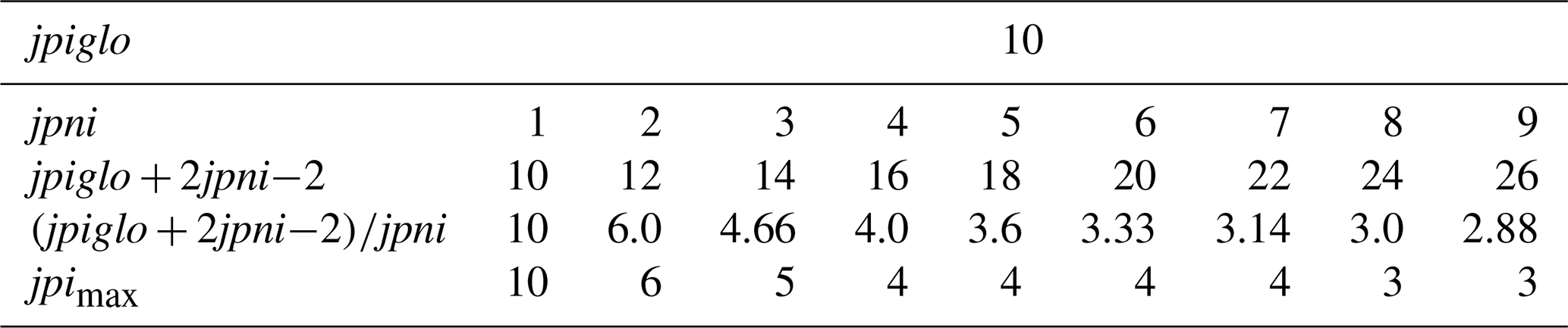
The second step of our algorithm starts with the simple fact that domain decomposition uses Euclidean division: the division of the horizontal domain by the number of processes along i and j directions rarely results in whole numbers. In consequence, some MPI subdomains will potentially be 1 point larger in the i and/or j direction than others. Increasing the number of processes does not always reduce the size of the largest MPI subdomains, especially when using a large number of processes compared to the global domain size. Table 1 illustrates this point with a simple example: a 1D domain of 10 points (jpiglo) distributed among jpni tasks with jpni ranging from 1 to 9. Because of the halos required for MPI communications, the total domain size is $(\mathit{jpiglo}+\mathrm{2}\cdot \mathit{jpni}-\mathrm{2})$ that must be divided by jpni. One can see that using jpni=4 to 7 will always provide the same size for the largest subdomains: 4. Only specific values of jpni (1, 2, 3, 4 and 8) will end up in a reduction of the largest subdomain size and correspond to the optimized values of jpni that should be chosen. Using other values would simply increase the number of MPI subdomains that are smaller without affecting the size of the largest subdomain.

Table 1 Example of 1D 10-point domain decomposition.

This result must be extended to the 2D domain decomposition used in NEMO. When searching all couples (jpni,jpnj) that should be considered when looking for the optimal decomposition, we can quickly reduce their number by selecting jpni and jpnj only among the values suitable for the 1D decomposition of jpiglo along the i direction and jpjglo along the j direction. The number of these values corresponds roughly to the number of divisors of jpiglo and jpjglo, which can be approximated by $\mathrm{2}\sqrt{\mathit{jpiglo}}$ and $\mathrm{2}\sqrt{\mathit{jpjglo}}$. This first selection is thus providing about $\mathrm{2}\sqrt{\mathit{jpiglo}\times \mathit{jpjglo}}$ couples (jpni,jpnj) instead of the (jpiglo×jpjglo) couples that could be defined by default. Next, we discard from the list of couples (jpni,jpnj) all cases ending up with more subdomains than Nsub_max provided by the previous step.

The final part of this second step is to build the list of optimal decompositions, each one defined by a couple (jpni,jpnj), with a number of subdomains (jpni×jpnj) ranging from 1 to a maximum of Nsub_max. This work is done with an iterative algorithm starting with the couple $(\mathit{jpni},\mathit{jpnj})=(\mathrm{1},\mathrm{1})$. The recurrence relation to find element N+1 knowing element N of the list of optimal decompositions is the following: first, we keep only the couples (jpni,jpnj) for which the maximum subdomain size is smaller than the maximum subdomain size found for the element N. Next, we define the element N+1 as the couple (jpni,jpnj) that gives the smallest number of subdomains (jpni×jpnj). It rarely happens that several couples (jpni,jpnj) correspond to this definition. If the situation arises, we decide to keep the couple with the smaller subdomain perimeter to minimize the volume of data exchanged during the communications. This choice is quite arbitrary as NEMO scalability is limited by the number of communications but not by their volume. Limiting the subdomain perimeter should therefore have a very limited effect. We stop the iteration process once there is no longer a couple with a subdomain size smaller than the one selected at rank N.

Once this list of the best domain decomposition sorted from 1 to Nsub_max subdomains is established, it remains only to follow the third step of our algorithm to get the best subdomain decomposition (see Sect. 2.1.1).

2.1.4 Additional optimization to minimize the impact of the North Pole folding

The former work of Maisonnave and Masson (2019) showed that the specific North Pole folding used in global configurations (the tripolar ORCA family grids; Madec and Imbard, 1996) is a source of load imbalance as the processes located along the northern boundary of the domain must perform additional communications. Maisonnave and Masson (2019) reduced the extra cost of theses communications by minimizing the number of array lines involved in these specific communications. This development decreased the additional work load of the northern processes. We decided to go one step further by minimizing the size along the j direction of the northern MPI subdomains so they have less to compute and can perform their specific communications without creating (too much) load imbalance.

This optimization takes advantage of the Euclidean division of the global domain used to define the MPI subdomains (see Table 1). In the large majority of cases, this division has a non-zero remainder (r) which means that some subdomains must be bigger than the others. The idea is simply to set the j size of all MPI subdomains, except for the northern ones, to the largest value given by the Euclidean division (jpj_max) and to attribute the remaining points along the j direction to the northern subdomains. By default, the domain is split along the j direction with the following j decomposition: $r\times {\mathit{jpj}}_{\max }+(\mathit{jpnj}-r)({\mathit{jpj}}_{\max }-\mathrm{1})$. If the configuration includes the North Pole folding, we switch to the following j decomposition: $(\mathit{jpnj}-\mathrm{1}){\mathit{jpj}}_{\max }+{\mathit{jpj}}_{\mathrm{north}}$ with ${\mathit{jpj}}_{\mathrm{north}}={\mathit{jpj}}_{\max }-\mathit{jpnj}+r$. This trick allows us to minimize the j size of the northern subdomains without changing the size of the largest MPI subdomains. Note that a minimum of 4 or 5 points is required for jpj_north in order to perform the North Pole folding around the F point (jperio=6) or the T point (jperio=4).

Figure 1 Example of ORCA025 domain decomposition along the j direction (1021 points): (a) j size of the largest MPI subdomains (jpj_max, in grey) and of the northern MPI subdomains (jpj_north, in orange) according to the optimum number of MPI subdomains in the j direction (jpnj); (b) ratio ${\mathit{jpj}}_{\mathrm{north}}/{\mathit{jpj}}_{\max }$ in %.

Figure 1 illustrates this optimization applied to the ORCA025 grid, which contains 1021 points along the j direction. Note that, following the results illustrated in Table 1, we kept only the optimal values of jpnj, and hence the occurrence of discrete values along this axis. When jpnj is small (<20 in the ORCA025 case), jpj_north remains close to jpj_max and their ratio is higher than 90 %. This optimization seems here to be insufficient, but communications are usually not a bottleneck when using large MPI subdomains (jpj_max∼100 and above). The ratio ${\mathit{jpj}}_{\mathrm{north}}/{\mathit{jpj}}_{\max }$ is generally smaller for larger values of jpnj (>20). It reaches a minimum of 20 % for jpnj=36, but the main drawback of this simple optimization is that the ratio can reach very large values (>90 %) even for very large values of jpnj. The benefit of this optimization may therefore significantly vary even when slightly changing the j decomposition. This optimization is a first step to improving NEMO performances when using a configuration with the North Pole folding, and we are still exploring other pathways to find an optimization that would be adapted to all j decompositions. We could, for example, set the j size of the northern MPI subdomains before computing the j decomposition of the remaining part of the domain. This solution would, however, require a criterion to specify the most appropriate j size, which will necessitate further benchmarking work to quantify the remaining load imbalance and its dependency on the domain size, on the number of subdomains and very likely on the machine and its libraries.

2.2 The BENCH configuration

On top of finding the best domain decomposition, exploring the code numerical performance requires a proper benchmark. Preferably one that is easy to install and configure while keeping the code usage close to production mode.

The NEMO framework proposes various configurations based on a core ocean model: e.g., global (ORCA family) or regional grids, with different vertical and horizontal spatial resolutions. Different components can moreover be added to the ocean dynamical core: sea ice (i.e., SI3) and/or bio-geo-chemistry (i.e., TOP-PISCES). A comprehensive performance analysis must thus be able to scrutinize the subroutines of every module to deliver a relevant message about the computing performance of the NEMO model to the whole user community. On the other hand, as pointed out by the former RAPS consortium (Mozdzynski, 2012), performing such benchmarking exercise must be kept simple, since it is often done by people with basic knowledge of NEMO or physical oceanography (e.g., HPC experts and hardware vendors).

We detail in this section a new NEMO configuration we specifically developed to simplify future benchmarking activities by responding to the double constraint of (1) be light and trivial to use and (2) allow any NEMO configuration to be tested (size, periodicity pattern, components, physical parameterizations…). At the opposite of the dwarf concept (Müller et al., 2019), this configuration encompasses the full complexity of the model and helps to address the current issues of the community. This BENCH configuration was used in Maisonnave and Masson (2019) to assess the performance of the global configuration (ORCA family). We use it in the current study section to continue this work and but also to improve the performance of the regional configurations.

2.2.1 BENCH general description

This new configuration, called BENCH, is made available in the tests/BENCH directory of the NEMO distribution.

BENCH is based on a flat-bottom rectangular cuboid, which allows any input configuration file to be by-passed and gives the possibility to define the domain dimensions simply via namelist parameters (nn_isize, nn_jsize and nn_ksize in namusr_def). Note that the horizontal grid resolution is fixed (100 km), whatever grid size is defined, which limits the growth of instabilities and allows the same time step length to be kept in all tests.

Initial conditions and forcing fields do not correspond to any reality and have been specifically designed (1) to ensure the maximum robustness and (2) to facilitate BENCH handling as they do not require any input file. In consequence, BENCH results are meaningless from a physical point of view and should be used only for benchmarking purposes. The model temperature and salinity are almost constant everywhere with a light stratification which keeps the vertical stability of the model. We add on each point of each horizontal level a perturbation small enough to keep the solution very stable while letting the oceanic adjustment processes occur to maintain the associated amount of calculations at a realistic level. This perturbation also guarantees that each point of the domain has a unique initial value of temperature and salinity, which facilitates the detection of potential MPI issues. We apply a zero forcing at the surface, except for the wind stress which is small and slowly spatially varying.

To make it as simple as possible to use, the BENCH configuration does not need any input file, so that a full simulation can be performed by downloading only the source code. In addition, the lack of input (or output) files prevents any disk access perturbation of our performance measurement. However, output can be activated as in any NEMO simulation, for example to test the performance of the XIOS (Meurdesoif, 2018) output suite.

2.2.2 BENCH flexibility

Any NEMO numerical scheme and parameterization can be used in BENCH. To help the user in his namelist choices and to test diverse applications, a selection of namelist parameters is provided with BENCH to confer to the benchmarks the numerical properties corresponding to popular global configurations: ORCA1, ORCA025 and ORCA12.

The SI3 sea-ice and TOP-PISCES modules can be turned on or off by choosing the appropriate namelist parameters and CPP keys when compiling. The initial temperature and salinity definition was designed in such a way that if SI3 is activated in the simulation, the sea ice will cover about one-fifth of the domain, which corresponds approximately to the annual ratio of ORCA ocean grid points covered by sea ice.

Any closed or periodical conditions can be used in BENCH and specified through a namelist parameter (nn_perio in namusr_def). The user can choose between closed boundaries, east–west periodical conditions, bi-periodic conditions (nn_perio=7) or even the North Pole folding used in the global configuration ORCA (nn_perio=4 or 6). Note that bi-periodic conditions ensure that all MPI subdomains have the same number of neighbor subdomains if there are no land points; it is a convenient way to reduce load imbalance. The specificity of the periodical conditions in ORCA global grids has a big impact on performance. This motivated the possibility to use them in the BENCH configuration: a simple change of nn_perio definition gives to BENCH the ORCA periodic characteristics and reproduces the same communication pattern between subdomains located on the northernmost part of the grid.

The above section describes the main BENCH features that are set by default, but we must keep in mind that each of them can be modified through namelist parameters if needed. By default, BENCH is not using any input file to define the configuration, the initial conditions or the forcing fields. We could, however, decide to specify some input files if it was required by the feature to be tested.

2.2.3 BENCH grid size, MPI domain decomposition and land-only subdomains

Like in any other NEMO configuration, BENCH computations can be distributed on a set of MPI processes. The BENCH grid size is defined in the namelist with two different options. If nn_isize and nn_jsize are positive, they simply define the total grid size on which the domain decomposition will be applied. This is the usual case, the size of each MPI subdomains is comparable (but not necessarily equal) for each MPI task and computed by the code according to chosen pattern of domain decomposition. If nn_isize and nn_jsize are negative, the absolute value of these parameters will now define the MPI subdomain size. In this case, the size of the global domain is computed by the code to fit the prescribed subdomain size. These options force each MPI subdomain to have the exact same size, whatever number of MPI processes is used, which facilitates the measurement of the model's weak scalability.

In NEMO, calculations are almost always performed at each grid point, and a mask is then applied to take into account land grid points if there are any. Consequently, the amount of calculations is the same with or without bathymetry, and it follows that the computing performance of BENCH and a realistic configuration are extremely close. However, we must underline that the absence of continents in the default usage of BENCH prevents the testing of the removal of subdomains entirely covered by land points (Molines, 2004). Note that it is possible to test a realistic bathymetry and the removal of land-only subdomains in BENCH by using any NEMO configuration input file in BENCH (as in all NEMO configurations). In this case, the user can simply define $\mathit{ln}\mathit{\_}\mathit{read}\mathit{\_}\mathit{cfg}=.\mathit{true}.$ and provide the configuration file name in the variable cn_domcf in the namelist block namcfg. A comparison of the BENCH scalability, without (named STD) or with land-only subdomains removal (named LSR), displayed in Fig. 2, was performed to assess the removal impact.

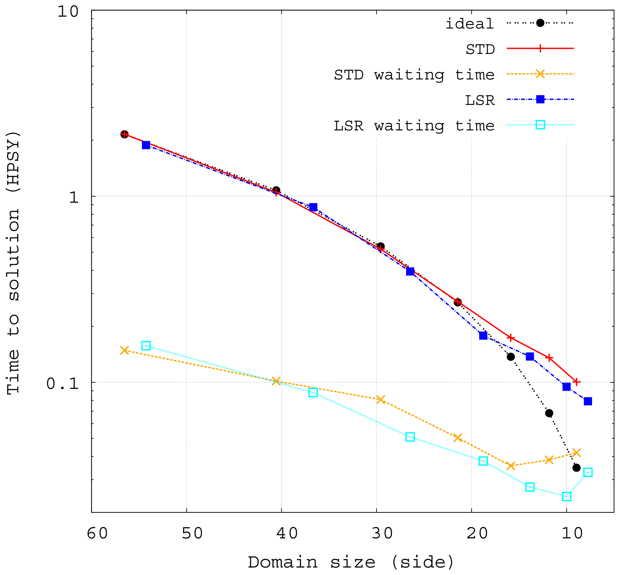
Figure 2 Time to solution (in hour per simulated year) as a function of the subdomain size (grid point number per subdomain side) on the BENCH configuration. The grid is the same as a global ocean grid at 1^∘ resolution (ORCA1). The configuration includes the SI3 sea-ice model. The STD case (red line) is without any bathymetry, the LSR case (dark blue line) has a bathymetry and land-only subdomains are removed. In each case, the waiting time is also plotted (orange and light blue).

Configurations that remove land-only subdomains might have smaller subdomains than configurations that do not when using the same number of MPI processes. A fair comparison of computing performance must hence be done with identical subdomain size. Therefore, the performance of Fig. 2 is not given as a function of the number of resources used, like in usual scalability plots, but as a function of the number of grid points in the side of a subdomain (mean of the root square of the subdomain area). Performance is slightly better in the LSR case. The other information displayed in Fig. 2, the simulation waiting time, represents the total elapsed time spent in MPI communications. The waiting time encompasses data transfer, overhead of the MPI library and computation load imbalance. The comparison of waiting time between STD and LSR helps to understand the origin of the small overall performance discrepancy. In the LSR case, some subdomains have land-only neighbors that they do not communicate with; this can explain LSR's shorter waiting time and some of the difference regarding the time to solution. However, scalability regimes, slopes and limits, for both time to solution and waiting time, are practically the same in STD and LSR. As already mentioned (Ticco et al., 2020), BENCH is able to reproduce the computation performance of any usual NEMO configuration and provides a simplified alternative for benchmarking work.

Since the 4.0 version release, the BENCH configuration was tested on various platforms and showed good numerical stability properties (Maisonnave and Masson, 2019). The stability of the BENCH configuration allows us to perform innovative benchmarks to easily test the potential impact of future optimization of MPI communications. BENCH can indeed run for quite a large number of time steps even if we artificially decide to skip MPI communications. For example, it is possible to examine the code scalability without any communication by simply adding a RETURN command at the beginning of NEMO communication routine. If we add an IF test with a modulo to decide if this RETURN command is applied or not, one can have an idea of what the code performance would be if we could reduce the communications by a factor of N. Likewise, one can test the potential benefits of plenty of ideas without getting too deep into the implementation.

2.3 Dedicated tool for communication cost measurement

The last piece of the puzzle that we implemented to set up an effective benchmarking environment in NEMO is to collect and summarize information related to the performance of the MPI part of the code.

In NEMO, MPI communications are wrapped in a small number of high-level routines co-located in a single Fortran file (lib_mpp.F90). These routines provide functionalities for halo exchange and global averages or min/max operations between all subdomains. With very little code changes in this file, it is possible to identify and characterize the whole MPI communication pattern. This instrumentation does not replace external solutions, based on automatic instrumentation, e.g., with “Extrae-Paraver” (Prims et al., 2018) or “Intel Trace Analyzer and Collector” (Koldunov et al., 2019), which provide a comprehensive timeline of exchanges. The amount of information collected by our solution is much smaller and the possibilities of analysis reduced, but we are able to deliver, without any external library, additional computing cost or additional postprocessing, simplified information on any kind of machine.

A counter of the time spent in MPI routines is incremented at any call of an MPI send or receive operation (named “waiting time”). A second counter handles MPI collective operations (named “waiting global time”). Additionally, a third counter is incremented outside these MPI-related operations (named “computation time”). On each process, only three data are collected into three floats: the cumulative time spent sending and receiving, gathering MPI messages, and the complementary period spent in other operations.

After a few time steps, we are able to produce a dedicated output file called communication_report.txt. It contains the list of subroutines exchanging halos, how many exchanges each perform per time step and the list subroutines using collective communications. The total number of exchanged halos, the number of 3D halos, and their maximum size are also provided.

At the end of the simulation, we also produce a separated counting, per MPI process, of the total duration of (i) halo exchanges for 2D and 3D as well as simple and multiple arrays, (ii) collective communications needed to produce global sum, min and max, (iii) any other model operation independent from MPI (named “computing”) and (iv) the whole simulation. These numbers exclude the first and last time steps, so that any possible initialization or finalization operations were excluded from the counting. This analysis is output jointly to the existing information related to the per-subroutine timing (timing.output file). This analysis can be found below the information related to the per-subroutine timing in the timing.output file.

3 Reducing or removing unnecessary MPI communications

This section presents the code optimizations that were done following the implementation of the benchmarking environment described in the previous section.

In a former study (Maisonnave and Masson, 2019) relied on the measurement tool (Sect. 2.3) to assess the performance of the BENCH configuration (Sect. 2.2). This work focused only on global configurations with grid sizes equivalent to 1 to $\mathrm{1}/\mathrm{12}$^∘ horizontal resolution that may or may not include sea-ice and bio-geo-chemistry modules. Maisonnave and Masson (2019) modified various NEMO subroutines to reduce (or group) MPI exchanges with a focus on the North Pole folding. In this section, we propose to complement the work of Maisonnave and Masson (2019) by improving NEMO's scalability in regional configurations instead of global configurations. This implies the configuration the BENCH namelist in a regional setup including open boundaries, as detailed in the Appendix A. We also deactivated the sea-ice component which was deeply rewritten in NEMO version 4 and necessitates a dedicated work on its performance.

As evidenced by Tintó et al. (2019), the MPI efficiency in NEMO is not limited by the volume of data to be transferred between processes but by the number of communications itself. Regrouping the communications that cannot be removed is therefore a good strategy to improve NEMO's performance. Our goal is thus to find the parts of the code which do the most communications and then figure out how we can reduce this number either by removing unnecessary communications or by grouping indispensable communications. Note that following the development of Tintó et al. (2019) a Fortran generic interface has been added to NEMO that makes the grouping of multiple communications extremely easy.

In the configuration we are testing (BENCH with no periodicity, open boundaries and no sea-ice), almost 90 % of communications are in two routines: the surface pressure gradient computation (44 %) and the open boundary conditions (45 %). The following optimizations will therefore focus on those two parts of the code. Note that in both cases, the involved communications transfer a very limited volume of data (from a single scalar to a 1-dimension array) which justifies even more the strategy proposed by Tintó et al. (2019).

3.1 Free surface computation optimization

In most of the configurations based on NEMO, including in our BENCH test, the surface pressure gradient term in the prognostic ocean dynamics equation is computed using a “forward–backward” time-splitting formulation (Shchepetkin and McWilliams, 2005). At each time step n of the model, a simplified 2D dynamic is resolved at a much smaller sub-time step Δt_* resulting in a sub-time step m, with m ranging from 1 to M(≈50). This 2D dynamic will then be averaged to obtain the surface pressure gradient term.

In the previous NEMO version, each sub-time step completes the following computations.

$$\left\{\begin{array}{l}{\mathit{\eta }}^{m+\frac{\mathrm{1}}{\mathrm{2}}}=(\frac{\mathrm{3}}{\mathrm{2}}+\mathit{\beta }){\mathit{\eta }}^m-(\frac{\mathrm{1}}{\mathrm{2}}+\mathrm{2}\mathit{\beta }){\mathit{\eta }}^{m-\mathrm{1}}+\mathit{\beta }{\mathit{\eta }}^{m-\mathrm{2}}\\ {\stackrel{\mathrm{‾}}{U_h}}^{m+\frac{\mathrm{1}}{\mathrm{2}}}=(\frac{\mathrm{3}}{\mathrm{2}}+\mathit{\beta }){\stackrel{\mathrm{‾}}{U_h}}^m-(\frac{\mathrm{1}}{\mathrm{2}}+\mathrm{2}\mathit{\beta }){\stackrel{\mathrm{‾}}{U_h}}^{m-\mathrm{1}}+\mathit{\beta }{\stackrel{\mathrm{‾}}{U_h}}^{m-\mathrm{2}}\\ {\stackrel{\mathrm{̃}}{U_h}}^{m+\frac{\mathrm{1}}{\mathrm{2}}}=D^{m+\frac{\mathrm{1}}{\mathrm{2}}}{\stackrel{\mathrm{‾}}{U_h}}^{m+\frac{\mathrm{1}}{\mathrm{2}}}\mathrm{\Delta }e\\ \text{Communication 1}\text{on }{\stackrel{\mathrm{̃}}{U_h}}^{m+\frac{\mathrm{1}}{\mathrm{2}}}\\ {\mathit{\eta }}^{m+\mathrm{1}}={\mathit{\eta }}^m-\mathrm{\Delta }{t}_{*}\left[\text{div}\right({\stackrel{\mathrm{̃}}{U_h}}^{m+\frac{\mathrm{1}}{\mathrm{2}}})+P-E]\\ \text{Communication 2}\text{on }{\mathit{\eta }}^{m+\mathrm{1}}\\ {\mathit{\eta }}^{\prime }=\mathit{\delta }{\mathit{\eta }}^{m+\mathrm{1}}+(\mathrm{1}-\mathit{\delta }-\mathit{\gamma }-\mathit{ϵ}){\mathit{\eta }}^m+\mathit{\gamma }{\mathit{\eta }}^{m-\mathrm{1}}+\mathit{ϵ}{\mathit{\eta }}^{m-\mathrm{2}}\\ {\stackrel{\mathrm{‾}}{U_h}}^{m+\mathrm{1}}=\frac{\mathrm{1}}{D^{m+\mathrm{1}}}[D^m{\stackrel{\mathrm{‾}}{U_h}}^m+\mathrm{\Delta }{t}_{*}((\mathrm{1}-r)g{\text{grad}}_x\left({\mathit{\eta }}^{\prime }\right)\\ -D^{m+\frac{\mathrm{1}}{\mathrm{2}}}fk\times {\stackrel{\mathrm{‾}}{U_h}}^{m+\frac{\mathrm{1}}{\mathrm{2}}}+\stackrel{\mathrm{‾}}{G}\left)\right]\\ \text{Communication 3}\text{on }{\stackrel{\mathrm{‾}}{U_h}}^{m+\mathrm{1}}\end{array}\right.$$

Here, η is the sea surface height, $\stackrel{\mathrm{‾}}{U_h}$ is the speed integrated over the vertical, $\stackrel{\mathrm{̃}}{U_h}$ is the flux, $D^m=H+{\mathit{\eta }}^m$ is the height of the water column, Δe is the length of the cell, P is precipitation, E is evaporation, g is the gravity acceleration, f is the Coriolis frequency, k is the vertical unit vector and G is a forcing term. β, r, δ, γ and ϵ are constants.

NEMO uses a staggered Arakawa C grid; that is to say that some variables are evaluated at different locations. Zonal velocities are evaluated at the middle of the eastern grid edges, meridional velocities at the middle of the northern grid edges and sea surface height at the grid center. Due to this feature, spatial interpolations are sometimes needed to get variables at another location than the one they were initially defined on. For instance, η^m+½ must be interpolated from T to U and V points to be used in the equation ${\stackrel{\mathrm{̃}}{U_h}}^{m+\frac{\mathrm{1}}{\mathrm{2}}}=D^{m+\frac{\mathrm{1}}{\mathrm{2}}}{\stackrel{\mathrm{‾}}{U_h}}^{m+\frac{\mathrm{1}}{\mathrm{2}}}\mathrm{\Delta }e=(H+{\mathit{\eta }}^{m+\frac{\mathrm{1}}{\mathrm{2}}}){\stackrel{\mathrm{‾}}{U_h}}^{m+\frac{\mathrm{1}}{\mathrm{2}}}\mathrm{\Delta }e$. Since adjacent points on both sides of the grid cells are needed in the interpolation, η^m+½ cannot be directly interpolated on eastern U-point ghost cells (grey arrows in Fig. 3). Similarly, η^m+½ cannot be interpolated on northern V-point ghost cells. It entails that ${\stackrel{\mathrm{̃}}{U_h}}^{m+\frac{\mathrm{1}}{\mathrm{2}}}$ is not directly computed on eastern U-point and northern V-point ghost cells. “Communication 1” is therefore used to update ${\stackrel{\mathrm{̃}}{U_h}}^{m+\frac{\mathrm{1}}{\mathrm{2}}}$ on those ghost cells.

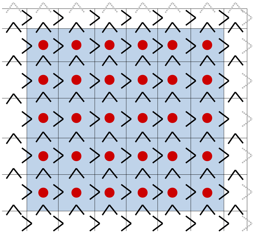
Figure 3 The MPI subdomain is bounded by the grid, the interior of the MPI subdomain is highlighted in blue while the ghost cells are in white. Black arrows show U and V points where η^m+½ (and therefore ${\stackrel{\mathrm{̃}}{U_h}}^{m+\frac{\mathrm{1}}{\mathrm{2}}}$) can be directly computed and grey arrows point where they cannot be computed without communication. Red dots show T points where $\text{div}\left({\stackrel{\mathrm{̃}}{U_h}}^{m+\frac{\mathrm{1}}{\mathrm{2}}}\right)$ can be directly computed.

The computation of $\text{div}\left({\stackrel{\mathrm{̃}}{U_h}}^{m+\frac{\mathrm{1}}{\mathrm{2}}}\right)$ defined at T points requires values of ${\stackrel{\mathrm{̃}}{U_h}}^{m+\frac{\mathrm{1}}{\mathrm{2}}}$ on adjacent U and V points. It therefore cannot be completed on western and southern ghost cells, and “Communication 2” updates the field on those cells. Similarly, grad_x(η^′) cannot be computed over the whole MPI subdomain, hence the “Communication 3”.

A careful examination of this algorithm is, however, showing that this communication sequence can be improved. As detailed in Fig. 3, the computation of $\text{div}\left({\stackrel{\mathrm{̃}}{U_h}}^{m+\frac{\mathrm{1}}{\mathrm{2}}}\right)$ (red dots) defined at T points only demands correct values at the four adjacent U and V points (black arrows). Values of η^m+½ on U and V points of northern and eastern ghost cells are not needed in the computation of $\text{div}\left({\stackrel{\mathrm{̃}}{U_h}}^{m+\frac{\mathrm{1}}{\mathrm{2}}}\right)$ on the interior of the MPI subdomain. Communication 1 on ${\stackrel{\mathrm{̃}}{U_h}}^{m+\frac{\mathrm{1}}{\mathrm{2}}}$ can hence be delayed and grouped together with Communication 2 on η^m+1. Note that the communication on ${\stackrel{\mathrm{̃}}{U_h}}^{m+\frac{\mathrm{1}}{\mathrm{2}}}$ cannot be removed altogether as the variable is also used for other purposes that are not detailed here.

Following this improvement, the number of communications per sub-time step in the time-splitting formulation has been reduced from 3 to 2. This translates to a reduction from 135 (44 %) to 90 (29 %) communications per time step in the surface pressure gradient routine for the examined configuration.

3.2 Open-boundary communication optimization

Configurations with open boundaries require fields on the boundaries to be changed frequently. In the previous NEMO version, a communication had to be carried out after the computation of boundary conditions to update values that are both on open boundaries and on ghost cells. In the configuration we tested, with open boundaries and no sea ice, 45 % of the number of communications was due to open boundaries.

Boundary conditions in NEMO are often based on the Neumann condition, $\frac{\partial \mathit{\varphi }}{\partial n}=\mathrm{0}$, where ϕ is the field on which the condition is applied and n the outgoing normal, or the Sommerfeld condition $\frac{\partial \mathit{\varphi }}{\partial t}+c\frac{\partial \mathit{\varphi }}{\partial n}=\mathrm{0}$, where c is the speed of the transport through the boundary. For both boundary conditions the only spatial derivative involved is $\frac{\partial \mathit{\varphi }}{\partial n}$. The focus is therefore to find the best way to compute $\frac{\partial \mathit{\varphi }}{\partial n}$ in various cases.

NEMO allows two kinds of open boundaries: straight open boundaries and unstructured open boundaries. As straight open boundaries along domain edges are far more common and easier to address, we will examine them first.

3.2.1 Straight open boundaries along domain edges

Figure 4a shows schematic representation of the BENCH configuration with straight open boundaries on every side that will be used to explain the optimizations performed in this part of the code. The code structure of NEMO requires domains to be bordered by land points (in brown) on all directions except when cyclic conditions are applied. The four open boundaries (red stripes on each side of the domain) are thus located next to the land points, on the second and before last rows and columns of the global domain.

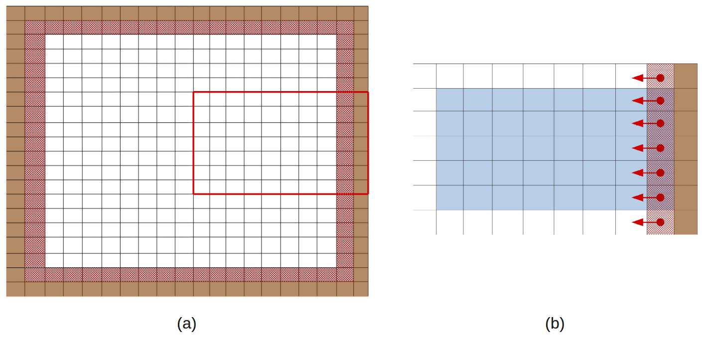
Figure 4 On the left, a configuration with straight open boundaries, the red line delimits a possible MPI subdomain detailed on the right. Brown cells are land cells and red hatched cells are open boundary cells. On the right, inner domain cells are in blue; red dots mark T points constituting the open boundary ((x_i,y_i)) and red arrows the points orthogonal to the boundary ($(x_{i-\mathrm{1}},y_i)$) used in the computing of $\frac{\partial \mathit{\varphi }}{\partial n}{|}_{(x,y)=(x_i,y_i)}$.

Let us consider an MPI subdomain located on the eastern side of the global domain, represented by the red square in Fig. 4a and detailed in Fig. 4b. Originally, the treatment of the open boundaries was performed only in the inner domain (red stripes over blue cells), and a communication phase was used to update the value on the ghost cells (red stripes over white cells). In the case of a straight longitudinal boundary with the exterior of the computational domain on the east, $\frac{\partial \mathit{\varphi }}{\partial n}{|}_{(x,y)}$ will be calculated at a point (x_i,y_i) by $\frac{\mathit{\varphi }(x_{i-\mathrm{1}},y_i)-\mathit{\varphi }(x_i,y_i)}{{\mathrm{\Delta }}_{x_{i,i-\mathrm{1}}}}$, where ${\mathrm{\Delta }}_{x_{i,i-\mathrm{1}}}$ is the distance between x_i and x_i−1. When such conditions are applied, only values defined at points orthogonal to the open boundary are needed, yet such points are inside the MPI subdomain, even when (x_i,y_i) is on a ghost cell (red stripes over white cells in Fig. 4b). Moreover, in the code, fields are always updated on ghost cells before open boundary conditions are applied; hence the entire field on the MPI subdomain is properly defined and can be used. The computation of the boundary condition is thus possible over the whole boundary including on ghost cells. There is no need for any communication update. When straight open boundaries along domain edges are used, this optimization gets rid of all the communications linked with open boundary computation.

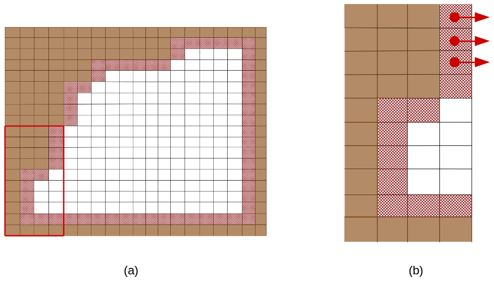
Figure 5 (a) A configuration with straight open boundaries on the eastern and southern sides and unstructured open boundaries on the western and northern sides; the red line delimits a possible MPI subdomain detailed in panel (b). Brown cells are land cells and red hatched cells are open boundary cells. Red dots mark some T points of the open boundary ((x_i,y_i)) and red arrows the points orthogonal to the boundary used in the computing of $\frac{\partial \mathit{\varphi }}{\partial n}{|}_{(x,y)=(x_i,y_i)}$.

3.2.2 Unstructured open boundaries

Unstructured open boundaries allow the user to define any boundary shape. Figure 5a shows an example of such an open boundary defined next to land points. A possible use of an unstructured open boundary is the following: a user could want the simulation not to include ocean points where the ocean is too shallow and instead define an unstructured open boundary delimiting an area of low depth (for instance in the vicinity of an island). The shallow ocean points will be defined as land points in the domain definition, but exchange of water masses and properties will be possible through the unstructured open boundary.

Depending on the MPI decomposition, open boundary cells can end up on ghost cells and facing the outside of the MPI subdomain, hence rendering direct computation of the boundary condition impossible. For example, in the MPI subdomain Fig. 5b, to compute the boundary condition $\frac{\partial \mathit{\varphi }}{\partial n}{|}_{(x,y)=(x_i,y_i)}$ on some points (x_i,y_i) highlighted by a red arrow would require the value of ϕ on a point ($(x_{i+\mathrm{1}},y_i)$) outside of the MPI subdomain. Note that straight open boundaries can potentially be defined anywhere in the domain (and not only along the domain edges). In this case it is also possible that a straight open boundary would be just tangential to the MPI domain decomposition. In such rare case, applying the open boundary conditions would also require a MPI communication. These rare cases are in fact treated in the same manner as for the unstructured open boundaries and are thus automatically included in the procedure we implemented for unstructured open boundaries.

We chose to detect points where direct computation (i.e., without a communication phase) will be impossible during the initialization of the model and trigger communications only for MPI subdomains where at least one such point is present. This allows for the previous optimization to be compatible with unstructured open boundaries. Points on a corner of an unstructured open boundary also require specific attention when tracking points that could need a communication phase. Indeed, on an outside corner, several points can be considered orthogonal to the open boundary. The choice of the neighboring points involved in this computation will tell us if the treatment of the corner requires a MPI communication or not. When reviewing the corner-point treatment in older NEMO version, we realized that the method chosen in some cases did not ensure symmetry properties (a reflection symmetry could change the results). We therefore decided to first correct this problem in the physical application of the Neumann condition of corner points before finding and listing those which require a MPI communication. This first step is detailed in the next paragraph even if, formally, this is not a performance optimization.

Applying the Neumann condition, $\frac{\partial \mathit{\varphi }}{\partial n}=\mathrm{0}$, to an open boundary point equates to setting that point to the value of one (or the average value of several) of its neighbors that are orthogonal to the open boundary. The selected method must have reflection and rotation symmetry properties and allow the open boundary point to be set to the most realistic value possible. The method used is illustrated in Fig. 6 where contour lines of a field ϕ are in blue with the ϕ=0 contour line passing through the T point of an open boundary cell (red dot) on an outside corner of the open boundary. Contour lines are straight and the field is increasing linearly in diagonal or orthogonal directions. Red arrows indicate the best choice for the Neumann condition. In Fig. 6 the best choice is to take the average of the values of the closest available points. Here, applying the Neumann condition is done by setting ϕ(x_i,y_i) to $\frac{\mathit{\varphi }(x_{i+\mathrm{1}},y_i)+\mathit{\varphi }(x_i,y_{i-\mathrm{1}})}{\mathrm{2}}$. Indeed, if only one of those two points were used, there would not be good symmetry properties (cases 1, 3 and 4), and if the top right point was also taken into the average, the result would be a bit better in case 1 for a nonlinear field but worse in cases 2, 3 and 4.

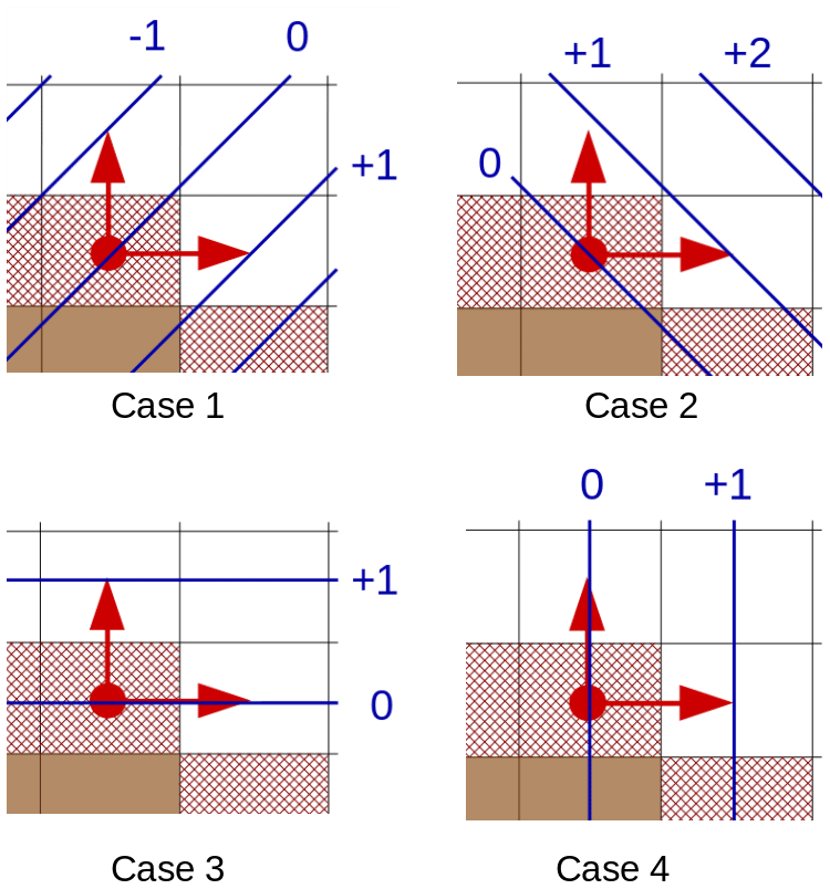
Figure 6 Brown cells are land cells and red hatched cells are open boundary cells. Red dots mark points from the open boundary and red arrows the best points to use to compute the Neumann condition, blue lines are contour lines of ϕ with the value of the contour line highlighted in blue.

Using the same method, we finally summarized all Neumann conditions and their neighbor contributions in five cases shown in Fig. 7. All other possible dispositions are rotations of one of these 5 cases. Thanks to this classification, we have next been able to figure out, from the model initialization phase, the communication pattern required by the treatment of the Neumann conditions. Based on this information we can restrict the number of communication phases to their strict minimum.

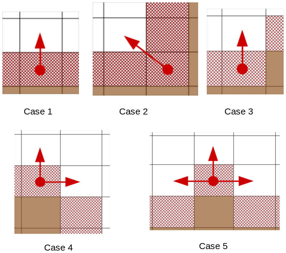
Figure 7 Brown cells are land cells and red hatched cells are open boundary cells. Red dots mark points from the open boundary and red arrows the points used in the computing of $\frac{\partial \mathit{\varphi }}{\partial n}{|}_{(x,y)=(x_i,y_i)}$ for the Neumann condition.

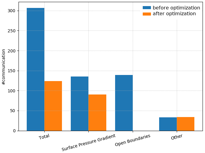
Figure 8 Comparison between the number of communications needed at each time step in NEMO before (blue) and after the optimizations of this section were carried out (orange) for a configuration with open boundaries and without ice.

3.3 Performance improvement

The performance is estimated using a realistic simulation of the West Atlantic between 100 and 31^∘ W and 8^∘ S and 31^∘ N. It includes continents and straight open boundaries on the north, east and south. The simulation is to the 32th of a degree with $\mathrm{2188}\times \mathrm{1300}=\mathrm{2}\mathrm{844}\mathrm{400}$ mesh cells and 75 vertical levels. To reduce the impact of the file system on the measurements, the simulation does not produce any output.

In this test case, which is representative of the very large majority of uses, the open boundaries are straight and located along the edge of the domain. The communications related to open boundaries have therefore been completely removed, and the communications related to the surface pressure gradient are reduced by a third. As a result, in this configuration, the total number of communications per time step has been reduced by about 60 % (Fig. 8).

The number of cores used is in line with the optimum dynamic sub-domain decomposition described in Sect. 2.1. For each core number, 3 simulations of 1080 time steps were conducted, and the computing time was retrieved at each time step of the model. Figure 9 shows that there are many outliers in the computing time that shift the mean to higher values while the median is not sensible to it. As the exact same instructions are run at every time step, the outliers are likely to be a consequence of instabilities of the supercomputer or preemption. A finer analysis showed that the slowdowns occur on random cores of the simulation. Since the median effectively filters out outliers it corresponds to the computing time one would get on an extremely stable supercomputer with no preemption.

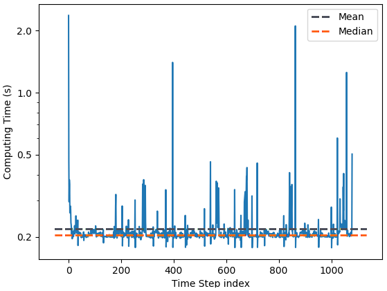
Figure 9 Computing time (in seconds) per time step for a West Atlantic simulation run with 2049 cores. The grey (orange) dashed line shows the mean (median) computing time of one time step.

Figure 10 shows the improvement of NEMO strong scaling brought by our optimizations. In this figure, the model performance is quantified by the number of years that can be simulated during a 24 h period (simulated years per day, SYPD). For small numbers of cores, the optimizations have no noticeable effect, as the time spent in communications is very small. However, as the number of cores rises, each MPI subdomain gets smaller, the computational load diminishes, and the communication load becomes predominant. Here the optimizations bring clear improvements: the number of simulated years per day is higher in the optimized version of the code (orange curves are above the corresponding blue curves). The scalability curves built by considering the 1080 time steps (solid lines) are nevertheless quite noisy, and the improvement is not as good as expected: 20 % at best with a negative value around 30 000 cores.

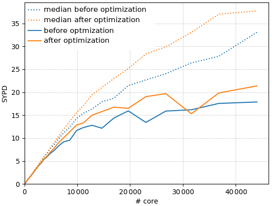
Figure 10 Strong scaling performance: simulated years per day (SYPD) as a function of the number of cores used in the simulation.

Filtering out the outliers by using the median gives results that are better and more robust. The resulting scalability curves (dashed lines) are less noisy. Moreover, if we except the last point, the distance between the two dashed lines is steadily increasing as we use more cores. The impact of our optimizations is therefore greater at greater core number. The number of SYPD is, for example, increased by 35 % for 37 600 cores when using the optimized version. One can also note that the optimized version that ran on 23 000 cores simulates the same number of SYPD as the old version on 37 600 cores, which represents a reduction of resource usage of nearly 40 %.

The differences between filtered and unfiltered results are possibly linked to instabilities. As each core has similar chances of suffering from instabilities or going into preemption, at higher core number slower cores are more common. Since communications tend to synchronize cores, a single slow core slows down the whole run. The median gets rid of time steps in which preemption or great instabilities occur. It indicates the performance we could get on a “perfect” machine which would not present any “anomalies” during the execution of the code. Such a machine unfortunately does not exist. The trend in new machine architecture with increasing complexity and heterogeneity suggests that performance “anomalies” during the model integration may occur more and more often to become a common feature. Our results point out this new constraint which is already eroding a significant part of our optimization gains (from 40 % to 20 %) and will need to be taken into account in the future optimizations of the code.

4 Conclusions

We presented in this paper the new HPC optimizations that have been implemented in NEMO 4.0, the current reference version of the code. The different skills we gathered among the co-authors allowed us to improve NEMO performance while facilitating its use. The automatic and optimized domain decomposition is a key feature to perform a proper benchmarking work, but it also benefits all users by selecting the optimum use of the available resources. This new feature also points out a possible waste of resources to the users, making them aware of the critical impact of the choice of the domain decomposition on the code performance. The new BENCH test case results from a close collaboration between ocean physicist and HPC engineers. We distorted the model input, boundary and forcing conditions to ensure enough stability to do benchmark simulations in any configuration with as few input files as possible (basically the namelist files). Note that the stability of this configuration even allows developers to carry out some unorthodox HPC tests. For example, artificially suppressing a part of the MPI communications to test the potential benefit of further optimizations before coding them.

In this 4.0 release, code optimization was targeting the scalability by reducing the number of communications. The present paper focuses on two parts of the code: (1) the computation of the surface pressure gradient that amounted to about 150 communications per model time step and (2) the treatment of the open boundaries conditions that was also doing a similar number of communications. We managed to reduce the communications by 30 % in the routine computing the surface pressure gradient. The results are even more spectacular in the part of the code dealing with the open boundaries as we managed to suppress all communications in the very large majority of cases. Note that this optimization work also gave us the opportunity to improve the algorithm used in the treatment of some unstructured open boundaries with a tricky geometry. Several conclusions can be drawn from the analysis of the performance improvements obtained with this very large reduction (from ∼300 to ∼125, that is to say ∼60 %) of the total number of communications per model time step. First, as expected, this optimization has an impact only once we use enough cores (>500 in our case), so the communications have a significant weight in the total elapsed time of the simulation. Second, the elapsed time required to perform one model time step is far from being constant as it should be in theory. Some time steps are much longer to compute than the median time step. This significant spread in the model time step duration requires that we use the median instead of the mean value when comparing performance of different simulations.

These results are suggesting further investigations for future optimizations. The large variability of the elapsed time needed for one time step suggests that the performance of the machines is definitely not constant. They are, in fact, varying in time and between the cores in a manner that is much larger than what we originally expected. This behavior can be explained by many things (preemption, network load, etc.). Benchmarks on different machines are suggesting that this heterogeneity in the functioning of supercomputers will get more common as we start using more cores. Code optimizations will have to take this new constraint into account. We will have to adapt our codes in order to absorb or limit the effects of asynchrony that will appear during the execution on the different cores. The way we perform the communication phase in NEMO, with blocking communications between, first, east–west neighbors and, next, north–south neighbors will have to be revisited, for example with non-blocking sending and receiving or with new features such as neighbor collective communications. In recent architecture, the number of cores inside a node has increased. This leads to a two-level parallelism where the communication speed and latency differs for inter-node exchanges and intra-node exchanges. Inter-node communications are probably slower and possibly a source of asynchrony. A possible optimization could therefore be to minimize the ratio of inter-node to intra-node communications. Figure 11 illustrates this idea. The domain decomposition of NEMO is represented with each square being an MPI process and each node a rectangle of the same color. In this representation, the perimeter of a “rectangle-node” directly gives the number of inter-node communications (if we say to simplify that the domain is bi-periodic and each MPI process always has four neighbors). If we make the hypothesis that each node can host x² MPI processes, these x² processes are placed by default on a “line node” with a perimeter of 2x²+2. In this case, the ratio of inter-node to intra-node communications is $(\mathrm{2}{x}^{\mathrm{2}}+\mathrm{2})/\mathrm{4}{x}^{\mathrm{2}}$. Now, if we distribute the x² processes on a “square node”, the number of inter-node communications becomes 4x and the ratio $\mathrm{4}x/\mathrm{4}{x}^{\mathrm{2}}=\mathrm{1}/x$. If we take x=8 for 64-core nodes, we get a reduction of −75 % of the number of inter-node communications when comparing the line-node dispatch (130) with the square-node dispatch (32). The ratio of inter-node versus intra-node communications drops from 50 % to 12.5 %. These numbers are of course given for ideal cases where the number of cores per node is a square. We should also consider additional constraints like the removal of MPI processes containing only land points, the use of some of the cores per node for XIOS, the IO server used and NEMO. The optimal dispatch of MPI processes in a real application is not so trivial but the aforementioned strategy is an easy way to minimize the inter-node communications. This could be an advantage when we will be confronted with the occurrence of more and more asynchrony.

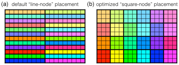
Figure 11 NEMO domain decomposition with the dispatch of the MPI processes among the different nodes. In this schematic representation, each square represents one MPI process of NEMO. We consider that NEMO is distributed over 216 MPI processes and that each node has 9 cores. The distribution of the MPI processes on the cores is represented by their color: processes on the same node have the same color. (a) Default dispatch of the MPI processes in lines; (b) optimized dispatch of the MPI processes in squares.

Appendix A: Namelist configuration to use BENCH with open boundaries

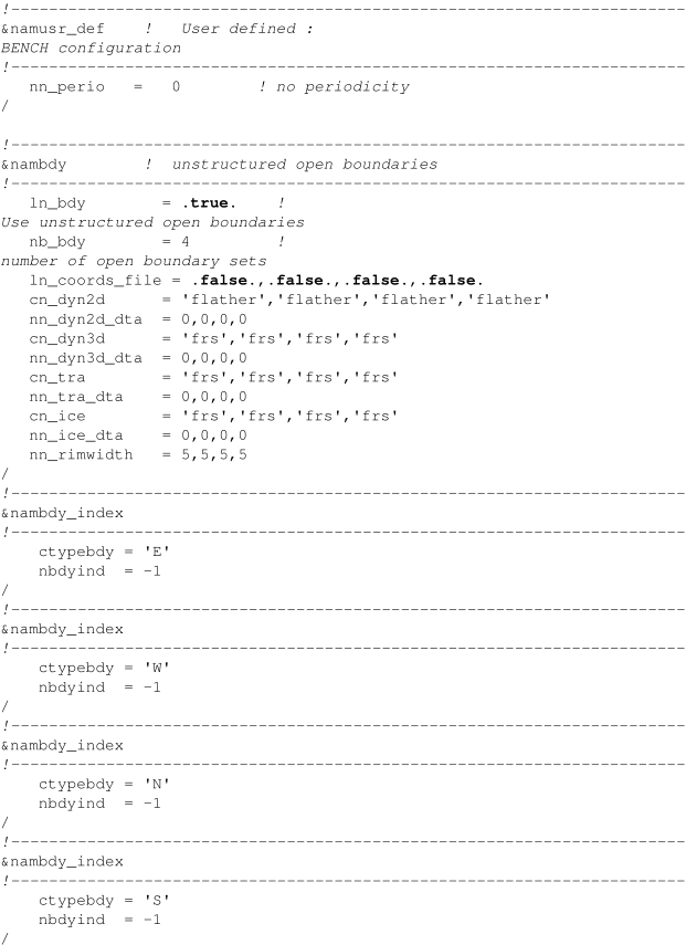
The BENCH configuration (see Sect. 2.2) was used by Maisonnave and Masson (2019) in its global configuration including the east–west periodicity and the North Pole folding. As detailed in Sect. 2.2.2, the BENCH configuration can be adapted to any purpose using the configuration file: namelist_cfg.

This appendix shows the parameters to be modified or added in namelist_cfg in order to use the BENCH configuration with straight open boundaries used in Sect. 3.