the Creative Commons Attribution 4.0 License.
the Creative Commons Attribution 4.0 License.
 | 10 Jan 2022
Importance of radiative transfer processes in urban climate models: a study based on the PALM 6.0 model system
Mohamed H. Salim
Sebastian Schubert
Jaroslav Resler
Pavel Krč
Björn Maronga
Farah Kanani-Sühring
Matthias Sühring
Christoph Schneider
Including radiative transfer processes within the urban canopy layer into microscale urban climate models (UCMs) is essential to obtain realistic model results. These processes include the interaction of buildings and vegetation with shortwave and longwave radiation, thermal emission, and radiation reflections. They contribute differently to the radiation budget of urban surfaces. Each process requires different computational resources and physical data for the urban elements. This study investigates how much detail modellers should include to parameterize radiative transfer in microscale building-resolving UCMs. To that end, we introduce a stepwise parameterization method to the Parallelized Large-eddy Simulation Model (PALM) system 6.0 to quantify individually the effects of the main radiative transfer processes on the radiation budget and on the flow field. We quantify numerical simulations of both simple and realistic urban configurations to identify the major and the minor effects of radiative transfer processes on the radiation budget. The study shows that processes such as surface and vegetation interaction with shortwave and longwave radiation will have major effects, while a process such as multiple reflections will have minor effects. The study also shows that radiative transfer processes within the canopy layer implicitly affect the incoming radiation since the radiative transfer model is coupled to the radiation model. The flow field changes considerably in response to the radiative transfer processes included in the model. The study identified those processes which are essentially needed to assure acceptable quality of the flow field. These processes are receiving radiation from atmosphere based on the sky-view factors, interaction of urban vegetation with radiation, radiative transfer among urban surfaces, and considering at least single reflection of radiation. Omitting any of these processes may lead to high uncertainties in the model results.
- Article
(15617 KB) - Full-text XML
- BibTeX
- EndNote


Urban climate models (UCMs) are useful tools to study the interaction between the urban environment and the atmosphere. They are broadly classified into two categories: the urban canopy-layer models and the urban boundary-layer models. The first category focuses on the microscale variations occurring below the canopy height (Maronga et al., 2020; Salim et al., 2018; Franke et al., 2012; Gross, 2012; Früh et al., 2011; Eichhorn and Kniffka, 2010; Huttner and Bruse, 2009). The second one examines the mesoscale variations occurring above the canopy height (Skamarock et al., 2019; Schlünzen et al., 2018; Jacob et al., 2012; Rockel et al., 2008). Over the last decades, the first category of UCMs has received an increasing interest as modern urban planning tools. They have been used to identify the implications of climate change for urban areas and to substantiate planning decisions as well as adaptation measures for climate change scenarios (Tumini and Rubio-Bellido, 2016; Crank et al., 2018; Geletič et al., 2019; Oswald et al., 2020). Also they have been used for a broad range of applications such as air pollution control, heat and wind comfort assessment, and general understanding of urban boundary-layer flows (Erell, 2008). The development of models has been mainly driven by recent advances in computer capacities, numerical algorithms, parameterization of micrometeorological processes, and data availability for urban structure (Masson et al., 2020). Together, these advances enabled UCMs to perform high-resolution simulations for large domains.
Modelling the radiative transfer processes (RTPs) within the urban domain is a key component in any UCM. It provides the surface radiation budget that is required for solving the surface energy balance. Indeed, an accurate prediction of surface radiation budget is fundamental to realistically model boundary-layer processes as it strongly affects turbulent surface heat fluxes (sensible and latent) (Xie et al., 2007), photolysis, and biometeorological parameters. However, modelling RTPs, which include radiation absorption, emission, reflection and scattering, in urban areas is a challenging task for many reasons. Firstly, the variation in surface material properties of different surface cover in an urban area (buildings, water, trees, etc.) generates a myriad of surfaces with different radiative properties such as emissivity and albedo. This makes it difficult to generate bulk radiative properties for urban areas (Oke, 1986). Secondly, the heterogeneity of shape and orientation of urban surfaces alters the incoming irradiance through many processes, such as shadow casting and multiple reflections. Thirdly, the radiative properties of the atmosphere are highly sensitive to air pollutants, clouds, and air temperature and humidity, which themselves are highly variable in urban areas (Verseghy and Munro, 1989a, b). Fourthly, modelling the RTPs is demanding in terms of radiative properties of urban surfaces and computational resources, which are not always available. Finally, the RTPs are non-local; i.e. urban surfaces may exchange radiation not only with other nearby surfaces but also with more distant surfaces. This poses technical difficulties to the numerical algorithms of those UCMs employing parallelization via horizontal domain decomposition (Resler et al., 2017).
For these reasons, it is excessively difficult to consider all the RTPs in UCM. Therefore, there exists a range of radiative transfer models (RTMs) of varying sophistication in the UCMs ranging from neglecting altogether the RTPs to parameterize most of the important RTPs in the canopy-height. However, there is little knowledge on how these models compare across a range of urban geometries and material properties encountered in an urban area. This knowledge is needed to estimate when these models are valid and how large the errors resulting from neglecting some of the RTPs in such models.
Many studies focused on the general effect of including solar radiation on the simulation of the flow field and pollutant dispersion in urban areas (Bottillo et al., 2014; Qu et al., 2012; Dimitrova et al., 2009; Xie et al., 2005; Archambeau et al., 2004). These studies used different methods to include thermal radiation. Some studies, e.g. Xie et al. (2005), used heated surfaces and other studies, e.g. Qu et al. (2011) and Archambeau et al. (2004), used embedded radiation models to provide the net atmospheric radiation flux for each solid surface. These studies showed that including solar radiation has significant effects on the flow field within the urban canopy layer (UCL) and on the associated processes, such as air pollution transport (Bottillo et al., 2014; Qu et al., 2012; Dimitrova et al., 2009; Xie et al., 2005; Archambeau et al., 2004). However, all these studies consider the radiative transfer in the canopy layer as a bulk process without distinguishing its inherent RTPs and most of them ignore some RTPs such as radiation reflections. To our knowledge, there is no study which evaluates the radiative transfer within an urban area by splitting down the RTPs and addresses their individual effects.
The main aim of this study is to investigate how much detail we should include to reasonably parameterize the radiative transfer in microscale building-resolving UCMs within the available computational resources. We introduce a generic method to individually evaluate the processes involved in the radiative transfer by isolating its effect on the surface radiative budget as well as the flow patterns. The comparison of the individual effects of each process allows an assessment of the applicability of the approximations applied in the UCMs. We focus on the major RTPs, such as the solid surface interaction with the incoming shortwave and longwave radiation, vegetation interaction with shortwave and longwave radiation, thermal emission of solid surfaces and vegetation, radiation reflection, and the interaction of vegetation with the reflected radiation. Those major RTPs exist in the commonly used UCMs. It is worth here mentioning that this study does not engage with validating the RTM of the Parallelized Large-eddy Simulation Model (PALM) against observations, which is the scope of other studies (Krč et al., 2021; Krč, 2019; Resler et al., 2017, 2021).
The paper is organized as follows: in Sect. 2, the methodology section, we provide a brief overview of the PALM model system and its RTM, which is employed in this study. We further describe in this section the stepwise parameterization method which is used to quantify the effect of each RTP process. The study cases and the quantification measures are described in Sect. 3. Section 4 presents the findings of the research, focusing on the key features that are modified by radiative transfer, i.e. the surface radiation budget and the flow field.
2.1 PALM 6.0 model system
The urban climate model adopted to this study is the PALM 6.0 model system. This model system is developed to be a modern and highly efficient model allowing for simulations over large domains (neighbourhood and city scale) with building-resolving spatial resolution (Maronga et al., 2019). It is based on the well-established large-eddy simulation (LES) PALM version 4.0 (Maronga et al., 2015). The model is further developed within the framework of the first phase of the funding programme “[UC2] – Urban climate under change”, funded by the German Federal Ministry of Education and Research (BMBF), to enhance the components needed for the application in urban environments (so-called PALM-4U components), such as interactive building surface and air quality schemes. Within the second phase of [UC2], PALM-4U is further developments to enhance its physical implementations, evaluation, and practicability. The model is briefly described below; however, for a detailed description, readers are advised to refer to Maronga et al. (2020).
The PALM model system solves the three-dimensional, non-hydrostatic, filtered, incompressible Navier–Stokes equations of wind (u, v, and w) and scalar variables (subgrid-scale turbulent kinetic energy, potential temperature, and specific humidity). These variables are staggered on an Arakawa-C Cartesian grid (Harlow and Welch, 1965; Arakawa and Lamb, 1977) with scalars defined at the centre of a grid box and the velocity components defined on the respective box faces. The Boussinesq approximation is applied to the filtered Navier–Stokes equations, and thus density variations are neglected except for the buoyancy term. The subgrid-scale turbulence parameterization depends on the mode of simulation being LES or the Reynolds-averaged Navier–Stokes (RANS).
The PALM model system includes all the modules required for simulating most of the atmospheric processes in complex urban areas (Salim et al., 2020). The plant canopy module accounts for the leaf–air interactions, such as the vertically extended drag, release of heat, and plant evapotranspiration for resolved vegetation such as trees and shrubs. The urban surface module (first version described by Resler et al., 2017) provides an energy balance solver for all urban elements (building walls, roofs, windows, green facades, pavements, etc.). The land surface module comprises an energy balance solver for natural (short non-grid-resolved vegetation, bare soil, and water) surfaces and pavements to realistically predict surface conditions and fluxes of sensible heat and latent heat as well as a multi-layer soil model to account for vertical diffusion (Maronga and Bosveld, 2017). The indoor climate module assesses the anthropogenic effects (i.e. air conditioning) on the urban atmosphere and predicts both indoor temperature as well as energy demand of buildings and waste heat. The chemistry module considers the chemical reactions, emission, deposition, and transport of substances, including reactive species to account for air pollution issues in urban environments. The biometeorological module evaluates the outdoor comfort of individuals in cities. The companion papers in this special issue as well as Maronga et al. (2020) give detailed descriptions of these model components.
The model exhibits excellent scalability on massively parallel computer architectures (Maronga et al., 2015). The model has been successfully evaluated against wind tunnel simulations, previous LES studies, and field measurements (Kanda et al., 2013; Letzel et al., 2008; Park et al., 2015; Razak et al., 2013).
2.2 Radiative transfer model
The RTM within PALM 6.0 system models the major shortwave (SW) and longwave (LW) radiative processes inside the UCL (Krč et al., 2021; Krč, 2019). In particular, it calculates the SW and LW irradiance received by all surfaces in the domain from the sky according to their orientation. This includes direct and diffuse shortwave irradiance and diffuse longwave irradiance from the atmosphere. To this end, it calculates for each surface a sky-view factor (SVF), using a ray-tracing algorithm, to adjust the radiation from the radiation model at the UCL top level to the respective surface. Also, it calculates the attenuation of SW irradiance due to vegetation (urban trees and shrubs) based on its leaf area density. Thus, the RTM calculates the plant canopy sink factor for each grid box containing leaves. For simplicity, vegetation is assumed to have zero heat capacity and the same temperature as the surrounding air, which is a common assumption in RTM approaches (Dai et al., 2003). The RTM also calculates the absorbed and the emitted SW and LW radiation from each surface, according to the surface properties, i.e. albedo and emissivity.
Another important process modelled by the RTM is the exchange of SW and LW irradiance by reflections, in the presence of vegetation. To enable this, RTM calculates mutual surface view factors (VFs). For computational reasons, however, the model uses a finite number of reflections (Krayenhoff et al., 2007) rather than infinite reflection (Yang and Li, 2013). Additionally, all surfaces are considered as Lambertian reflectors; hence, directional reflection is not considered.
In all these processes, the absorption, scattering, and thermal emission by air mass are neglected. Consequently, the model application in some weather situations such as fog, heavy precipitation, or dense smog is limited at the moment.
The RTM processes are briefly described in Sect. 2.4. However, the detailed description of the RTM is given in Krč et al. (2021) and in Krč (2019).
In order to perform this study, the PALM 6.0 model is edited to implement the stepwise parameterization method described in Sect. 2.4. In particular, switches were added to isolate the radiation processes according to the required step.
2.3 Radiation model and coupling
The Rapid Radiative Transfer Model for Global models (RRTMG; Clough et al., 2005) is used in PALM, and hence in this study, to provide the shortwave and longwave radiation components at the top of the urban canopy (highest obstacle, a building, or a tree, plus a height buffer). The RRTMG provides both the direct SW radiation flux and the diffuse downwelling SW and LW fluxes at this height. The recent development of the PALM model allows for a two-way coupling between the radiation model, the RRTMG in this case, and the RTM (Krč et al., 2021). For instance, the incoming SW and LW radiation fluxes from the RRTMG are used as inputs to the RTM so that all the RTPs are calculated and provided to the impeded models (e.g. urban and land surface model) for solving the energy balance. Simultaneously, the RTM provides three effective radiation surface parameters to the RRTMG, which are used as its boundary conditions: the effective surface temperature, the effective surface emissivity, and the effective surface albedo.
The RRTMG–RTM coupling is an important feature of PALM. In Sect. 4, we show how the RTPs integrated in the RTM do not only affect the surface radiation budget directly but also implicitly as these processes change the effective radiation surface parameters.
2.4 Stepwise parameterization method (SPM)
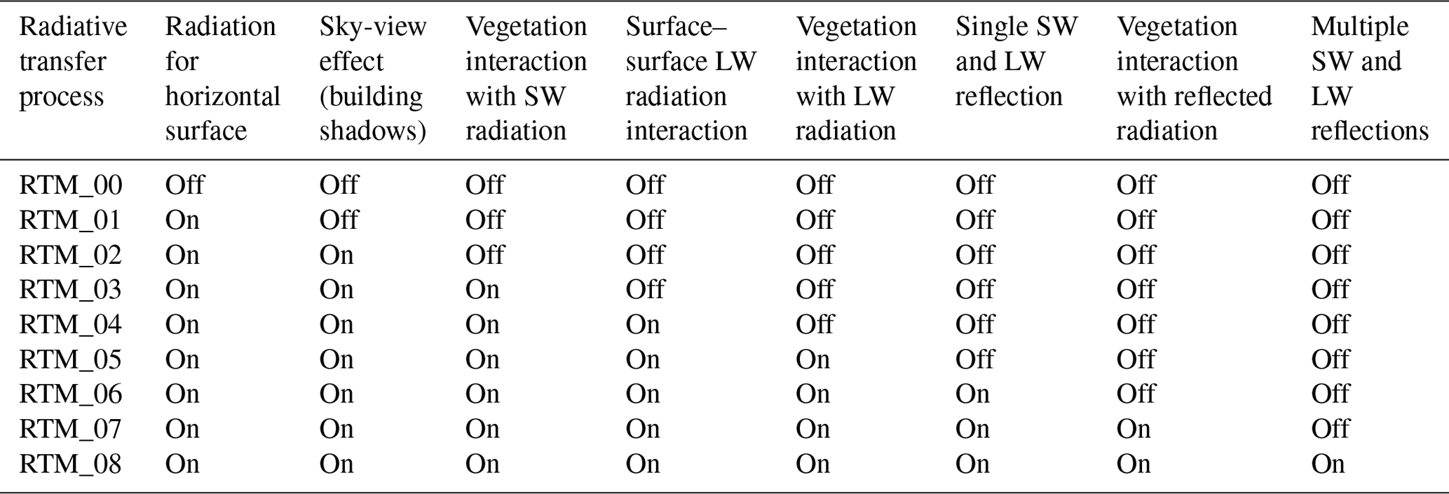
A bottom-up approach is used to put together the compositional sub-RTPs to give rise to the more complex RTM. In other words, a specific RTP is selected and integrated into the previous RTM to form the next RTM. Thus, the effect of adding this particular process to the RTM can be isolated and quantified. In this way, a series of RTMs with different sophistication emerged in a stepwise manner, starting from a simple RTM to the full RTM (Table 1). The order of adding the sub-RTPs to build up these RTMs depends on the degree of complexity needed to consider the RTPs and the expected effect of this process on the radiation budget. Each RTM is briefly described below.
Table 1Composition of radiative transfer processes (RTPs) for each radiative transfer model (RTM) used in the stepwise parameterization method (SPM).
2.4.1 No radiation (RTM_00)
Radiation is ignored altogether in this parameterization step so that there are no RTPs within the urban domain. This resembles the simulation of the neutral atmospheric boundary layer. Although radiation is ignored in this parameterization step, it is used here as a baseline for comparing the different RTPs.
2.4.2 Simple RTM (RTM_01)
All surfaces receive equal incoming radiation (SW and LW) from the radiation model without any interference with obstacles (buildings or trees). The value of the received radiation, ϕ, for a surface i is calculated so that the total incoming radiation from the radiation model, E, over the whole domain A is divided equally among all the surfaces, as follows:
where a is the surface area, N is the number of surfaces, including roofs, walls, and ground surfaces.
This means that both SVFs and VFs are not needed here. Although this simplification reduces the memory and the CPU time requirements considerably (see Sect. 2), major RTPs such as surface orientation, obstacle shadow, surface emission, reflections, etc. are missed out.
2.4.3 Sky view (RTM_02)
In this parameterization step, the RTM calculates the SVF of each grid-box face, to account for diffuse radiation, as well as shape factors to determine if, for a specific point in time, a face is exposed to direct sunlight. This will have a major influence on the surface-received SW and LW fluxes for two reasons. First the model can predict the shadow due to buildings, and second the model can prescribe proper SW flux from the Sun and LW flux from the atmosphere to the vertical surfaces. The incoming SW and LW fluxes are improved, compared to the simple RTM; however, they result in an increase in the runtime as well as the memory requirements to calculate SVFs. This RTM does not include the effect of trees on the radiative transfer.
2.4.4 Vegetation interaction with SW solar radiation (RTM_03)
Resolved vegetation (urban trees) is represented in the model as a porous media by its leaf area density (LAD). In this RTM, each grid box with a non-vanishing LAD, i.e. urban vegetation canopy box, absorbs part of the SW radiant flux passing through it, according to its transmittance (the factor that defines how much incoming radiation is passing through). The transmittance, T, is defined in PALM as , where a is the canopy box LAD, s is the length of ray's intersection with the plant canopy, and the constant α is the extinction coefficient, which is set to 0.6. The leaf thermal capacity is assumed to be zero, so that the absorbed radiation is directly transferred to air. Details on how the absorbed radiation is partitioned between sensible and latent heat flux are given in Krč et al. (2021).
2.4.5 Surface emission (RTM_04)
In this step, RTM allows all surfaces to receive LW radiation not only from the atmosphere but also from the outgoing LW radiation emitted from other building surfaces. According to the Stefan–Boltzmann law, a surface of a skin temperature Ts emits thermal radiation equal to ; here, ε is the emissivity and σ is the Stefan–Boltzmann constant. The amount of thermal radiation along with the reflected part of the LW radiation from the atmosphere will be transferred to other surfaces according to their VF. Thus, in addition to the SVFs, VFs for each surface to other surfaces must be calculated in advance. This process alone may increase the asymptotic computational complexity of a modelled domain, which has a horizontal size of (n×n), to O(n5) or O(n3), depending on the ray-trace discretization scheme (Krč, 2019). Also, surfaces may have mutual visibility, and hence exchange thermal radiation, even when they are far apart. As a result, this imposes further constrains on the memory layout of the parallelized models which use the Message Passing Interface (MPI) system for the parallel process communication. This represents a further increase in the runtime and the memory requirements.
2.4.6 Vegetation interaction with LW irradiance (RTM_05)
The interaction of vegetation with LW irradiance includes mainly two processes: thermal radiative emission from vegetation towards the urban surfaces and the sky and the absorption of LW radiation within the vegetation. Minor processes such as mutual LW radiative transfer and reflections within vegetation itself are neglected to save computations. Such an approximation is reasonable since vegetation in urban area usually has low reflectivity (high emissivity) in the longwave spectrum and similar surface temperature. The received irradiance of a surface j from a vegetation box i is calculated as
where VFi→j is the respective view factor, σ is the Stefan–Boltzmann constant, and Ti is the leaves' temperature (set to the surrounding air temperature). Here, the reflections in the plant canopy are ignored; hence, the emissivity of the leaves is set to 1, based on Kirchhoff's law. Thermal emission from vegetation towards the sky is similarly calculated using the SVFs of the vegetation boxes. The absorbed LW by a vegetation box i originating from face j is calculated as
where CSF is the canopy sink factor and Je,i is the radiosity of the surface. For the diffuse LW radiation from the sky, the radiosity of the surface is the diffuse LW radiation flux from the radiation model.
The extra geometrical factors required for this parameterization step, i.e. VF and CSF, are derived from the geometrical factors calculated for the previous parameterization steps. Detailed derivations for vegetation view and sink factors are given in Krč (2019). Although extra computational resources are needed to calculate these factors, the radiant flux emitted from vegetation towards each face must be exchanged among processors. This implies further runtime due to MPI communications.
2.4.7 Single reflection (RTM_06)
Urban surfaces in this parameterization step may receive reflected LW and SW irradiance in addition to the received irradiance from the main sources described above. Here, we enable only one iteration of reflection of LW and SW irradiance. This process is particularly important for the surfaces located in shadows because it is their source of SW irradiance along with the incoming diffuse SW radiation from sky. Also it enhances receiving LW irradiance along with receiving LW radiation from thermal emissions of other surfaces. The view factors needed for this step are already calculated (Sect. 2.4.5); however, the reflected LW and SW irradiance fluxes must be exchanged among processors, similar to RTM_05.
2.4.8 Vegetation interaction to reflected irradiance (RTM_07)
In this parameterization step, vegetation partially absorbs the reflected SW and LW radiation from all the surfaces where vegetation boxes exist between the target and the source surfaces. The absorbed radiation is directly released to the atmosphere since vegetation is assumed to have zero heat capacity. The irradiance absorbed by vegetation is calculated using CSF, similar to Sect. 2.4.6, and no MPI communication is needed here. The reflectivity of the vegetation is kept at zero.
2.4.9 Multiple reflections (RTM_08)
Four iterative reflections of LW and SW irradiance are applied in this RTM. The number of reflection iterations is chosen so that the absorbed radiation at the last reflection step is small enough so that any further reflections can be ignored (Krč et al., 2021). With each reflection step, surfaces receive radiation from the reflected LW and SW irradiance. In the meantime, vegetation partially absorbs this received radiation flux. With each reflection step, the reflected LW and SW irradiance fluxes need to be exchanged among processors, indicating higher runtime requirements.
This RTM represents the RTM version 3.0, which is used in PALM 6.0 model system. Since it contains all the RTPs covered in this study, we use it as a comparison RTM.
Two study cases are employed in this study. The first case has a rather simple geometry, while the second one has a realistic urban configuration. The test cases are designed to this study so that the changes due to each SPM step are explained first on a simple configuration and then demonstrated on a realistic case.
3.1 Simple urban configuration
Uniformly distributed buildings of cubic shapes are considered to represent a simple urban configuration with 16 buildings. However, imposing cyclic boundary conditions at the domain sides implicitly indicates unlimited domain. All buildings have the same size (building height H=20 m). The buildings are arranged so that they shape street canyons with an aspect ratio of 1. All surfaces between buildings are paved. The grid spacing is 1 m in the all directions. All surfaces in the domain (buildings and pavements) have the same surface characteristics. The albedo α and the emissivity ε for all surfaces are set to 0.15 and 0.9, respectively. This is intentionally done so that comparing the irradiance among surfaces is not biased by different surface characteristics.
All trees in the domain (24 trees in total) are identical in size and foliage density. They are uniformly distributed in the domain so that a tree is centred between two buildings. The following empirical equation, suggested by Lalic et al. (2013), is used to obtain the vertical distribution of LAD:
where z is the height of a grid box centre, h is the tree height, LADm is the maximum value of LAD, and zm is the height this maximum occurs (Lalic et al., 2013). In this formula, the constant n is set as follows to
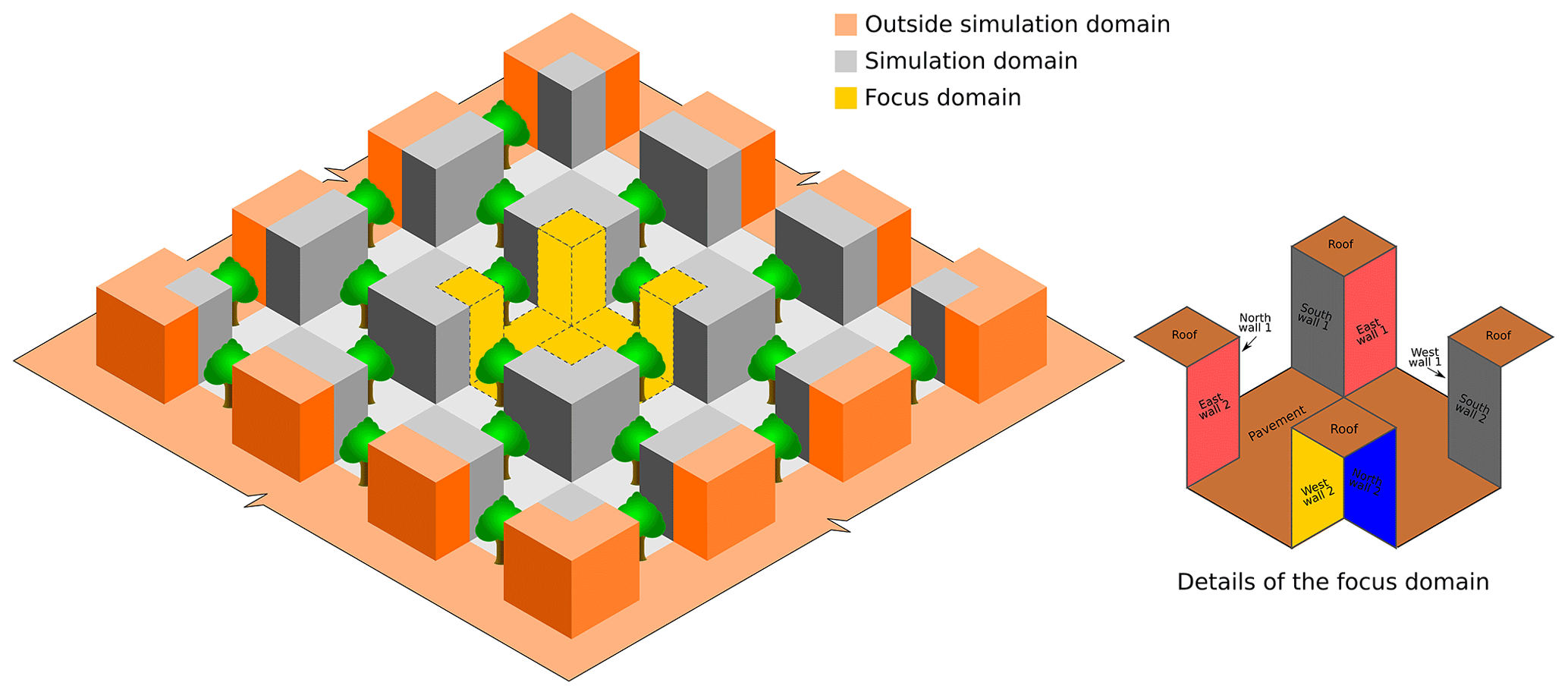
Figure 1Illustration of the simple urban configuration showing the simulation and the focus domain. The trees (shown in green) are centred between buildings.
Tree height, h, is set relative to the building size, H, so that and the LADm and values are assumed to be 1.6 m2 m−2 and 0.47, respectively. The crown diameter, Dtree, which describes how many grid boxes are occupied by one tree is set as . The wind direction is set to 270∘ (west wind). The street crossing located in the domain centre and parts of the buildings in its surrounding are chosen to be the focus domain. The building arrangement as well as the focus domain are shown in Fig. 1.
3.2 Realistic urban geometry
A domain extending 1×1 km2 around the town square – Ernst-Reuter-Platz located in Charlottenburg in Berlin (Germany) – is employed here to apply the SPM procedures to a realistic urban configuration, as shown in Fig. 2. This domain contains several features of urban complexity, such as different building heights, street configurations, trees, and open spaces. The available information of the real buildings as well as the trees located in the domain is utilized to integrate the buildings and trees into the computational grid. Moreover, the real orography heights as well as the surface cover characteristics of the domain are also included. All data are originally taken from the Geoportal Berlin and then preprocessed by the German Aerospace Centre (DLR) to meet the PALM input data standard (PIDS) (Heldens et al., 2020).
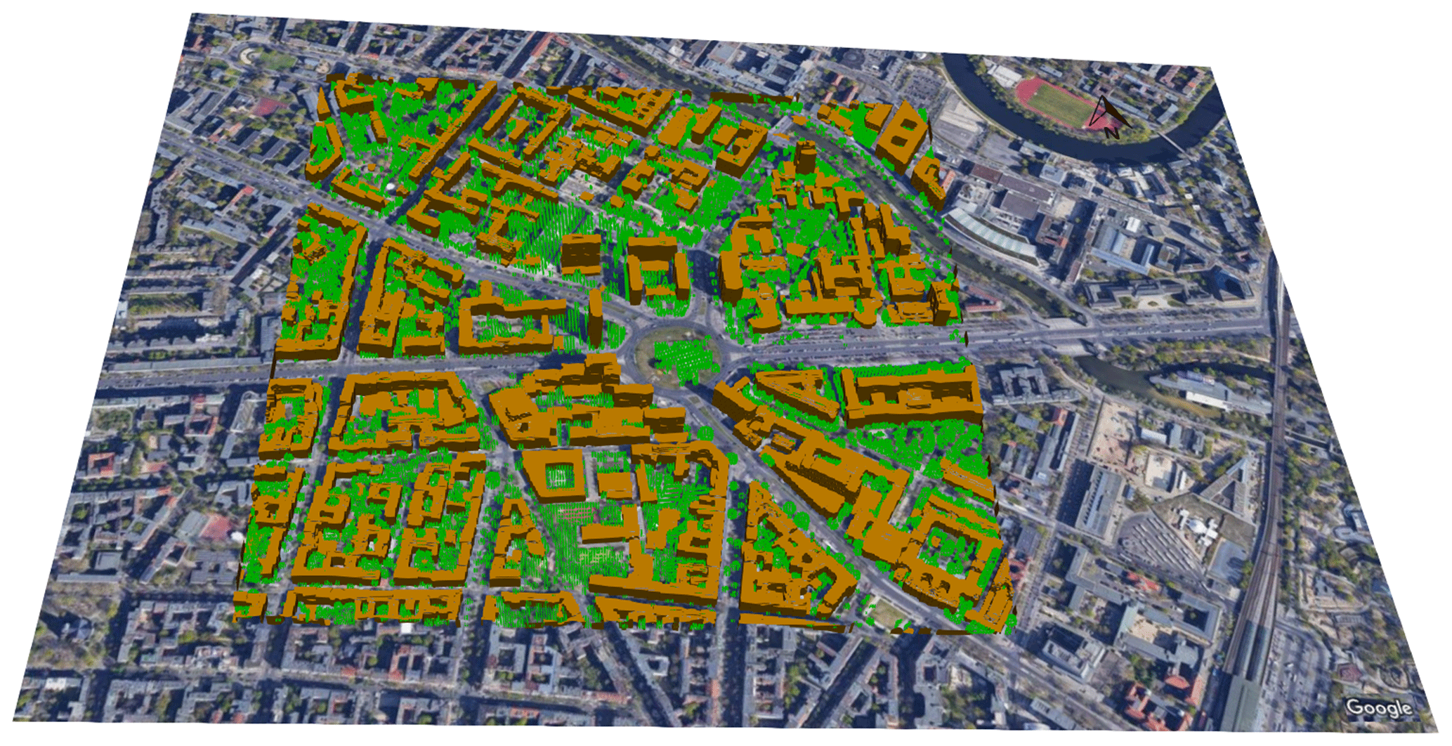
Figure 2An aerial view of the realistic urban configuration showing the 3-D buildings (fitted to the grid) and the plant canopy boxes (trees, shown in green points). The configuration is centred around Ernst-Reuter-Platz in Charlottenburg in Berlin (52∘30.8′ N, 48∘19.31′ E). The copyright for the underlying satellite image is held by © GeoBasis-DE/BKG 2009, Google 2009.
3.3 Quantification measures
In order to quantify the quality of each UCM, we introduce quantification measures that compare the model results of each step with the step before or with RTM_08, which contains all the RTPs considered in RTM version 3.0 (Krč et al., 2021). In order to eliminate the boundary bias, a focus domain is chosen so that surfaces near boundaries, which may receive radiation from the domain sides, are excluded from the analysis (Figs. 1 and 2).
3.3.1 Surface radiation flux
The individual RTPs are quantified by calculating the change of a relevant radiation flux, Δϕ, of a surface i due to including this process in the RTM, as follows:
where is a radiation flux for a surface i in the current RTM and is the flux using the previous RTM. This is done for each surface located in the focus domain every 1 h. The distribution of these differences is usually multimodal due to the surface orientations, thus, summary statistics such as mean/median and interquartile ranges are not meaningful. Therefore, the data are plotted using violin plots (Hintze and Nelson, 1998), which are similar to a box plot but with the addition of a rotated kernel density plot on each side.
3.3.2 Flow properties
For each SPM step, the change in the flow properties is evaluated using a relative error measure of a flow property magnitude (wind speed and air potential temperature) between the model results of this step and those based on RTM_08. A vector of relative error values is determined for all grid points located in the focus domain. The normalized root-mean-square error, nRMSE, of the relative error vector is used to provide a scalar measure of error in the flow properties for a particular SPM step,
where is the flow property at index when using SPM parameterization step, is its equivalent when using RTM_08, ψref is a reference property used for normalization, and N is the number of atmospheric grid points in the focus domain but excluding buildings.
The normalized volumetric flow rate, , is also used as a measure for quantitative comparisons of the flow field in the domain (Salim et al., 2015). This measure represents the vertical volume flow rate, Vz, through a horizontal plane at a height z above the ground normalized by the domain cross-sectional area Ad (omitting the buildings area), and a characteristic velocity U (e.g. undisturbed corresponding velocity at boundary-layer height). It is calculated as
Similar to nRMSEψ, only the focus domain is used to calculate to eliminate boundary effects.
These two measures, i.e. nRMSEψ and , quantify changes in the wind speed, both horizontal and vertical, but not the changes in the wind direction, which is not covered in the analysis.
The full 3-D simulations for all cases begin at 00:00 local solar time (LST) on 30 June and lasted for 2 d. No cloud formation is applied for all cases to ensure clear-sky conditions. Before the 3-D simulation, a precursor simulation for 1 d using the PALM spin-up mechanism was done for each case. This is done to properly initialize the surface temperature of all surfaces and to reduce the computational load. Further details on the spin-up mechanism in PALM is given in Maronga et al. (2020). The simulations of the simple case required between 2.86 and 3.11 wall-clock hours running on 100 computer cores, totalling between 286 and 311 CPU hours per simulation. The simulations of the realistic case were running on 1024 computer cores for 4.53 to 5.55 wall-clock hours. In total, the CPU hours ranged between 4644 and 5685 h per simulation.
4.1 Surface radiation fluxes for the simple case
Before proceeding to examine the effect of each RTP on the surface radiation budget, we discuss the incoming SW and LW radiation fluxes from the RRTMG radiation model at the top of the UCL (Fig. 3), which are used as input for the different RTM configurations used in the simulations. SW radiation peaks at midday with a value of 902 W m−2 and shows only subtle differences between the different RTMs of up to 15 W m−2 (Fig. 3a). Recalling the RRTMG–RTM coupling, this is not surprising since the effective urban parameters related to the SW radiation do not vary significantly for such a small configuration. LW radiation fluxes vary between 322 and 375 W m−2 and feature relatively larger differences of up to 53 W m−2 (Fig. 3b). Recalling again the RRTMG–RTM coupling, the incoming LW radiation from the RRTMG is affected by the effective urban parameters, i.e. the effective emissivity and temperature. These parameters are sensitive to the reflected, absorbed, and emitted surface LW radiation flux, which vary with each RTP added to the RTM.
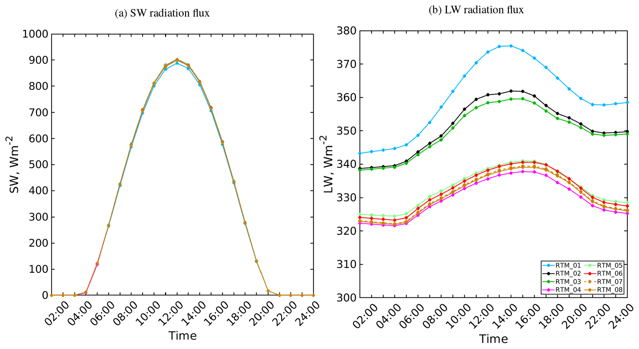
Figure 3The daily course of incoming (a) shortwave and (b) longwave radiation fluxes for the top of the urban layer of the simple urban configuration at 52∘ N on 1 July for different RTM configurations. Please note that the lines overlap in panel (a) due to the small relative changes in the incoming SW radiation.
In the next sections, we compare the surface radiation fluxes within the focus domain of both the simple and the realistic urban domains when applying the SPM procedures. We focus mainly on the incident SW and LW irradiance because they explicitly show the behaviour of RTM associated to each SPM step.
Beside the violin plots, we occasionally show examples of the spatial distribution of the changes in some relevant radiation flux components for the surfaces. The walls, the roof, and the pavements of the simple urban configuration are folded in a 2-D plot, showing the radiation flux changes in all the surfaces. The surface fluxes shown on these plots are based on the surface fluxes at 14:00 LST (instantaneous flux for SW radiation and hourly averaged flux for LW radiation). At this time, the surfaces are exposed to direct solar radiation and all surfaces are heated.
The figures are based on the surfaces located only in the focus domain to eliminate boundary effects. The number of surfaces in the focus domain of the simple configuration is 3200 surfaces (1600 vertical and 1600 horizontal surfaces of 1 m2 each).
4.1.1 Simple RTM (RTM_01)
The incident SW and LW irradiance for the surfaces in the focus domain are compared to those of the no-radiation-interaction case (RTM_00) (Fig. 4). Incidentally, the median and the average of the respective SW and LW values are identical because all the surfaces, regardless of their orientation, receive the same value of incoming radiation. Using this simple RTM overestimates the incoming SW flux in the shadow areas, where only the reflected and the diffuse SW fluxes are expected, and underestimates the incoming SW flux in the unshaded areas, especially the roof and ground surfaces. The incoming LW radiation from the sky is overestimated in the surfaces which have low sky visibility and underestimated for those having high sky visibility, due to averaging. Also all surfaces miss the LW emissions from building surfaces and trees as well as from LW reflections.
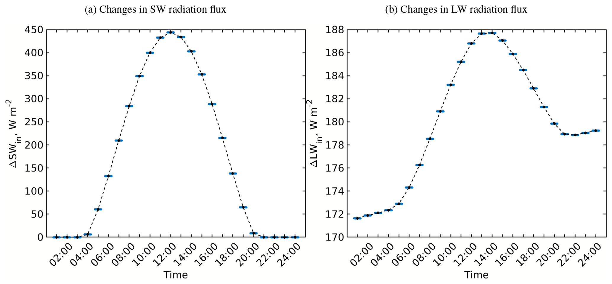
Figure 4Changes in the received SW and LW irradiance within the focus domain of the simple urban configuration when applying the simple RTM (RTM_01) compared to the neutral case (RTM_00). Since all surfaces receive the same radiation in the simple RTM, the violin plots appear as concentrated points. The mean values are shown by a dashed black line and the median values are shown by black circles.
4.1.2 Sky view (RTM_02)
The calculated SVFs and Sun visibility enable the model to more realistically predict the incoming direct and diffuse SW radiation flux from the Sun on both horizontal and vertical surfaces, giving rise to building shadows. Also, the SVFs adjust the received LW flux for the horizontal surfaces and add the corrected value to the vertical surfaces. In Fig. 5, the respective values of this case are compared to those predicted by RTM_01.
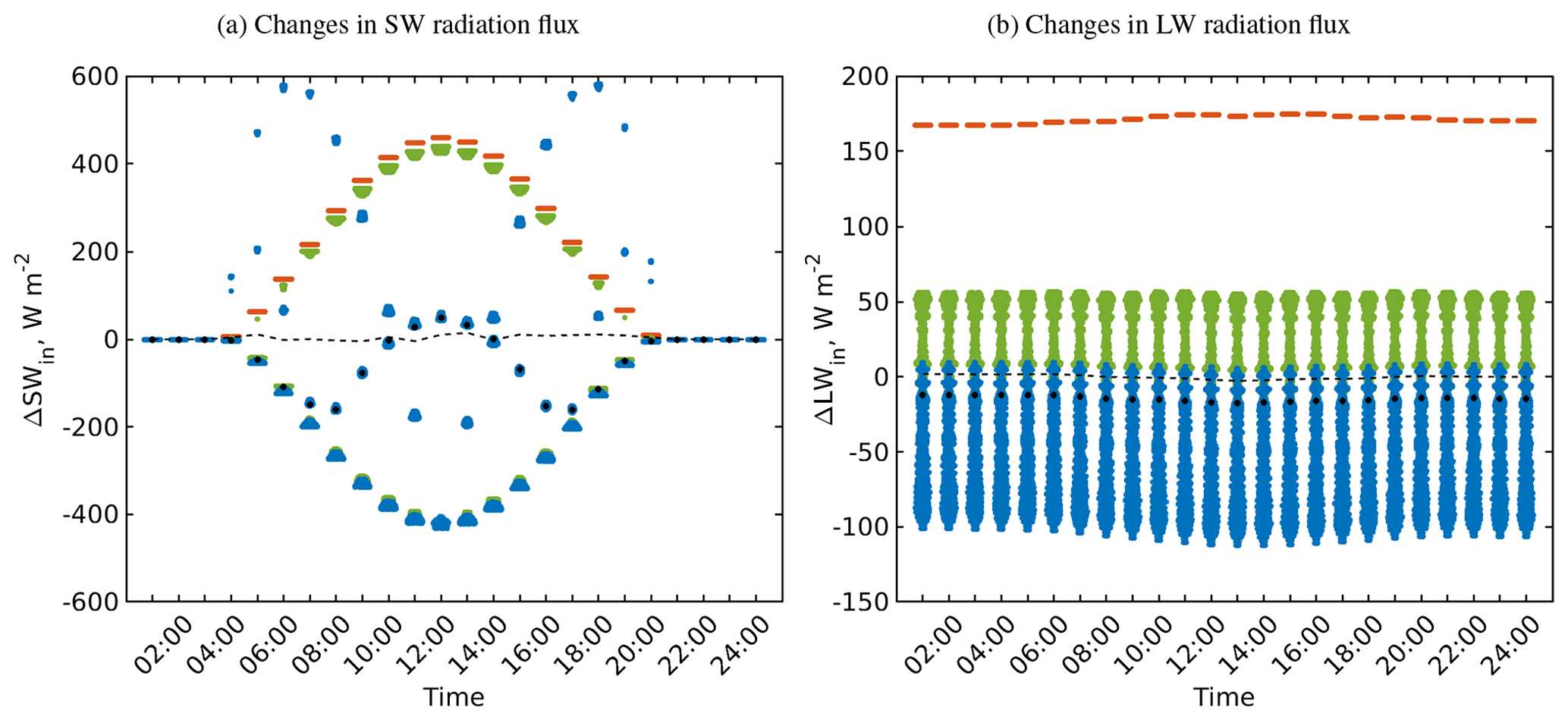
Figure 5Changes in the received SW and LW irradiance within the focus domain of the simple urban configuration when considering the surface sky-view factors (RTM_02) compared to the RTM_01. The roof, the wall, and the ground surfaces are shown in the violin plots in orange, blue, and green, respectively. Similar to Fig. 4, the mean values are shown by a dashed black line and the median values are shown by black circles.
Large changes in the SW radiation flux (±600 W m−2) result from the changes in the direct component. For instance, the negative high values are related to the surfaces located in the shadow, while the positive high values are related to the unshaded surfaces. The resulting relatively small values in the changes in mean SW irradiance stem from the changes in the diffusive component. Since surfaces have diverse SVFs, the changes of the diffusive SW component are accordingly distributed, unlike the direct SW component.

Figure 6Changes in the received LW radiation flux within the focus domain of the simple urban configuration when considering the surface sky-view factors (RTM_02) compared to the RTM_01. Walls (left plot), pavements (in the centre of the right plot), and roofs (rectangles on all four sides in the right plot) are folded. See the details of the focus domain of the simple urban configuration in Fig. 1.
The increased LW radiation flux (up to +175 W m−2) belongs mainly to the roof and pavement surfaces, which receive the full incoming LW radiation flux compared to the average value in RTM_01. The negative changes (up to −105 W m−2) are related to the wall and some pavement surfaces whose SVFs are reduced in the current parameterization step. Moreover, the received LW radiation changes implicitly due to the changes in the RRTMG's longwave radiation discussed above. This behaviour is summarized in the spatial distribution of the changes of the incident LW flux at 14:00 UTC in Fig. 6.
4.1.3 Vegetation interaction with SW irradiance (RTM_03)
The changes in the received SW and LW irradiance due to considering the vegetation interaction with the incoming SW radiation flux are shown in Fig. 7. The vegetation partially absorbs the incoming direct and diffuse SW flux components based on its LAD leading to a reduction of up to 900 W m−2. For direct SW irradiance, trees partly or fully cast shadows on the surfaces located in their shadow angle if they are not shaded by buildings anyway. Since direct SW irradiance is the dominant incoming flux during daytime, the radiation budget of the surfaces impacted by vegetation are highly changed. For diffuse SW irradiance, trees decrease the view factor of those surfaces located in their effective view area, and hence decrease the incoming diffuse SW irradiance as well. Since diffuse SW is not directional, all surfaces having trees in their view angle are affected, even if they are shaded by buildings (e.g. Fig. 8).
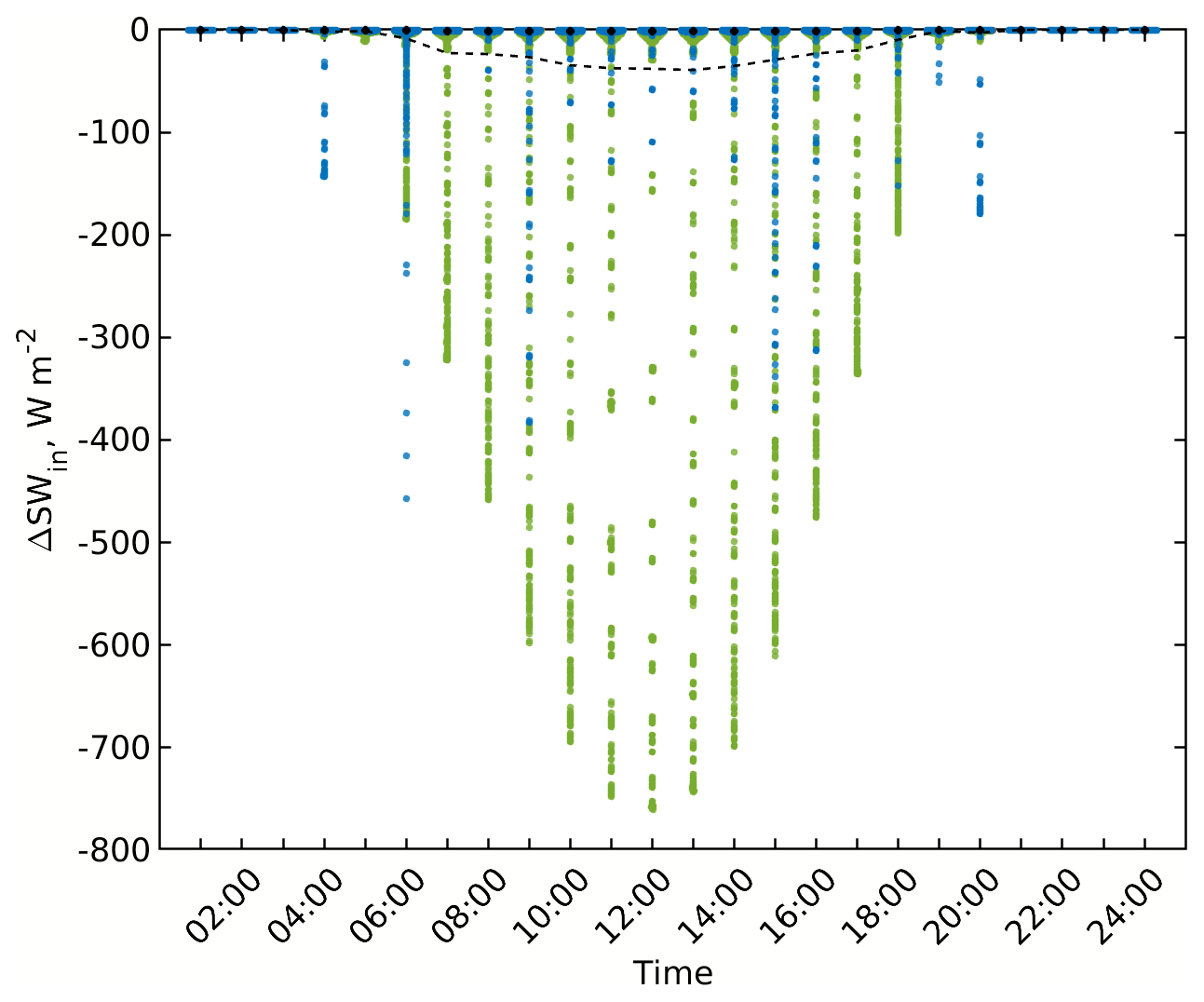
Figure 7Changes in the received SW irradiance within the focus domain of the simple urban configuration when considering vegetation interaction with SW solar radiation (RTM_03) compared to the RTM_02. Violin, mean, and median colours are used in the same way as those in Fig. 5.
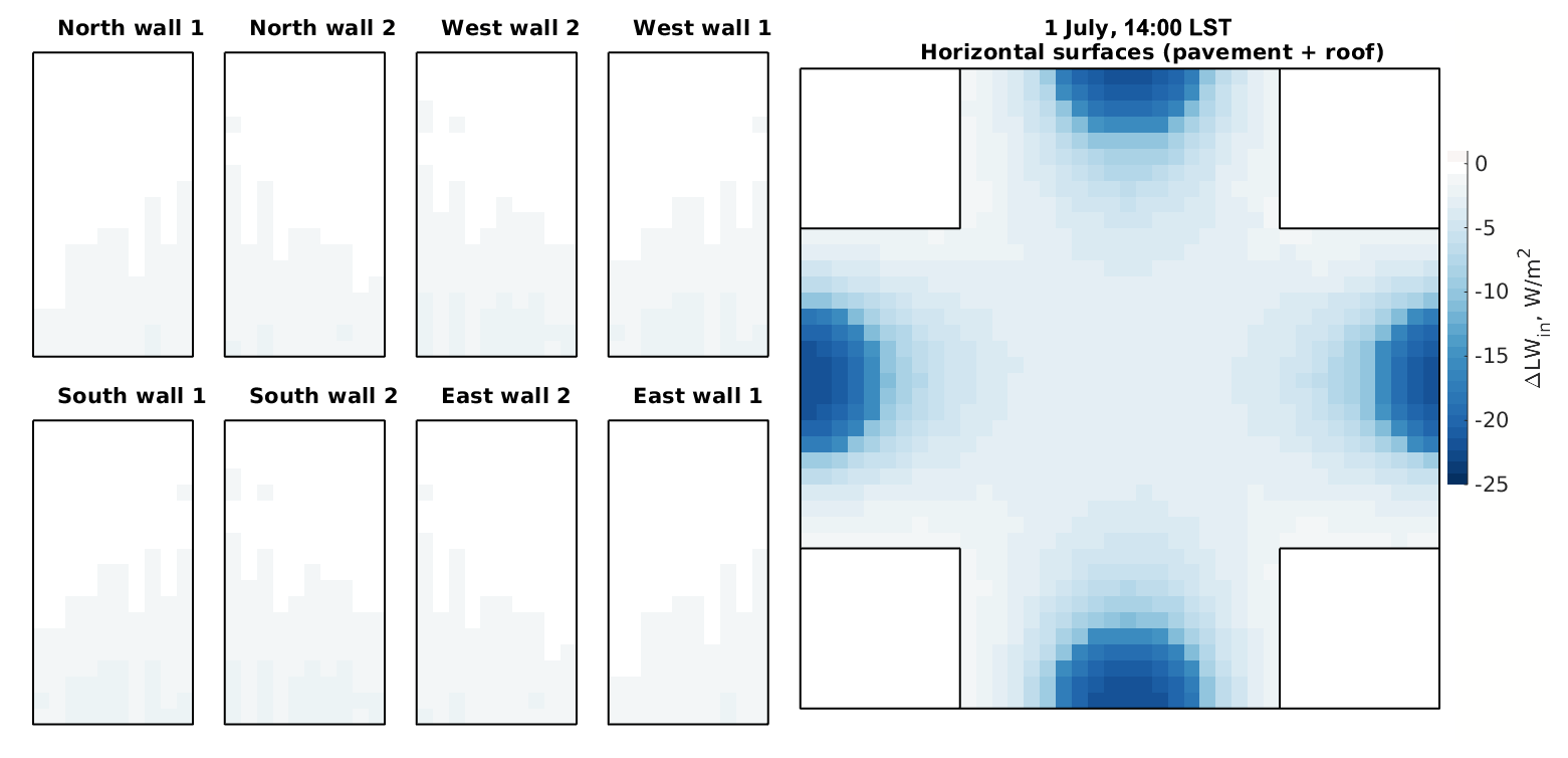
Figure 8Changes in the received diffuse SW radiation flux within the focus domain of the simple urban configuration when considering vegetation interaction with SW solar radiation (RTM_03) compared to the RTM_02. Walls, roofs, and pavements are folded the same way as those in Fig. 6.
Although this parameterization does not allow direct interaction of vegetation with LW radiation, slight changes in the incoming LW irradiance, compared to the previous step, are noticed. This is attributed to the changes in the incoming LW radiation from the radiation model (RRTMG) due to the RRTMG–RTM coupling, Fig. 3b.
4.1.4 Surface thermal emission (RTM_04)
The changes in the received LW irradiance shown in Fig. 9 are due to receiving thermal emissions from urban surfaces in the RTM. Most of the surfaces receive considerable amounts of LW radiation; nevertheless, some surfaces do not receive LW radiation from surface emissions. Those surfaces do have a vanishing view factor to any other surfaces (i.e. the roof surfaces, Fig. 10). What stands out in this configuration is the high value of received radiation flux even at nighttime, compared to RTM_03. This contribution to the surface radiation budget is considerable, and for some surfaces, especially those located in shadows, it is the main source of radiation.

Figure 9Changes in the received LW irradiance within the focus domain of the simple urban configuration when considering surface thermal emissions (RTM_04) compared to the RTM_03. Violin, mean, and median colours are used in the same way as those in Fig. 5.
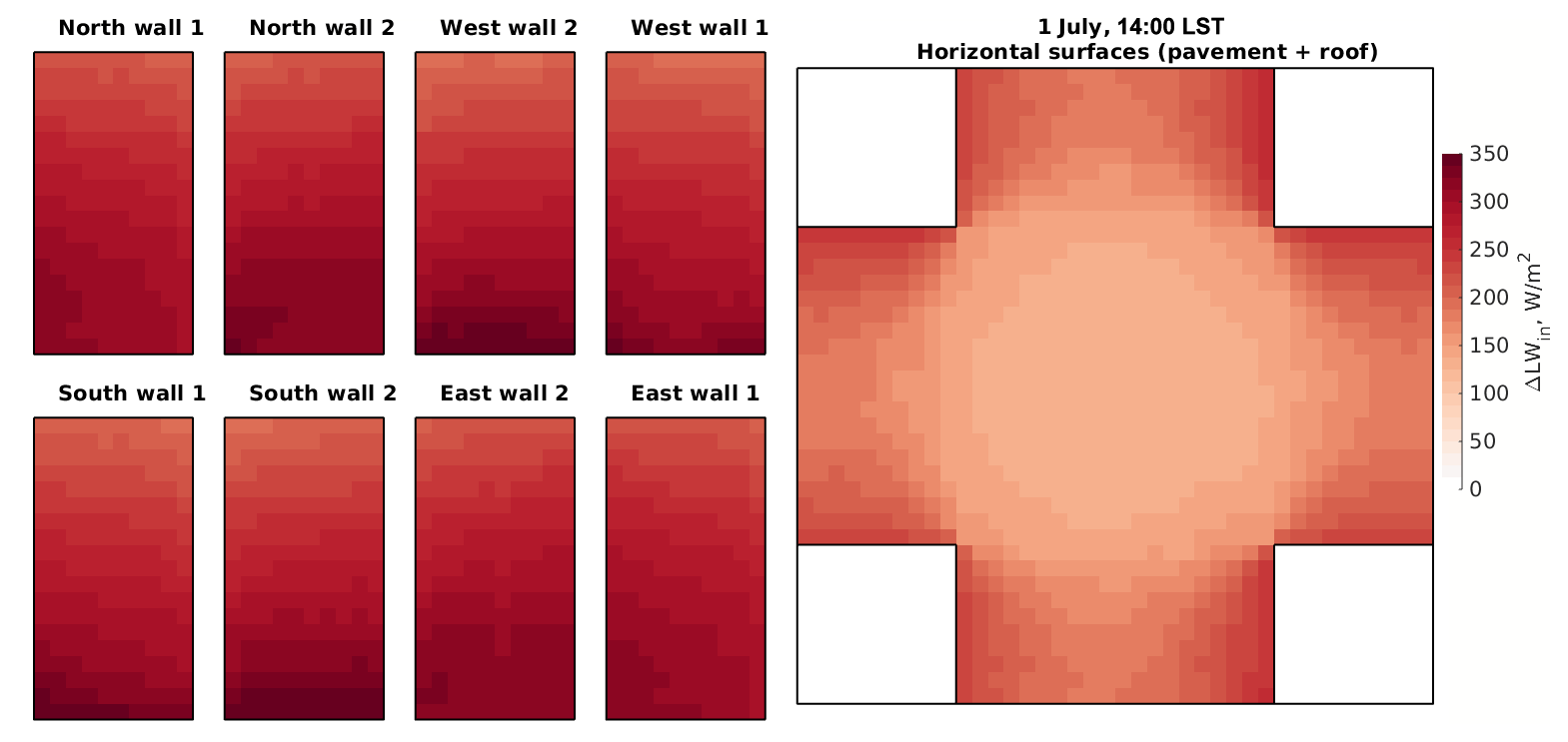
Figure 10Changes in the received diffuse LW radiation flux within the focus domain of the simple urban configuration when considering surface thermal emissions (RTM_04) compared to the RTM_03. Walls, roofs, and pavements are folded the same way as those in Fig. 6.
The SW radiation parameterization is not changed; hence, negligible changes less than 1 W m−2 in the received SW radiation flux are simulated (not shown here).
The considered process in RTM_04 has also an implicit implication on the radiation budget. For instance, when a surface receives extra LW irradiance from thermal emission of other surfaces, its surface temperature increases. Accordingly, the thermal emission from this particular surface increases with increasing the surface temperature to the power of 4 according to the Stefan–Boltzmann law. Thus, in turn, the other surfaces will receive higher LW irradiance as well.
Including this process decreases the incoming LW radiation from the atmosphere by about 1 W m−2 due to the coupling of RTM and RRTMG. In the previous steps, all the surface LW emission is emitted to the atmosphere, while in this step these emissions are only partially emitted to the atmosphere, leading to a lower effective surface temperature.
4.1.5 Tree thermal emission (RTM_05)
So far, the entire vegetation interaction with LW transfer has been ignored. The justification is that the absorbed LW radiation by vegetation may be compensated by the emitted LW radiation from vegetation. This simplification is acceptable provided that the surface temperature of the plant canopy is similar to the temperature of the surrounding surfaces. However, this is not always the case. Therefore, both the absorption and the emission of LW radiation by vegetation are included in this step.
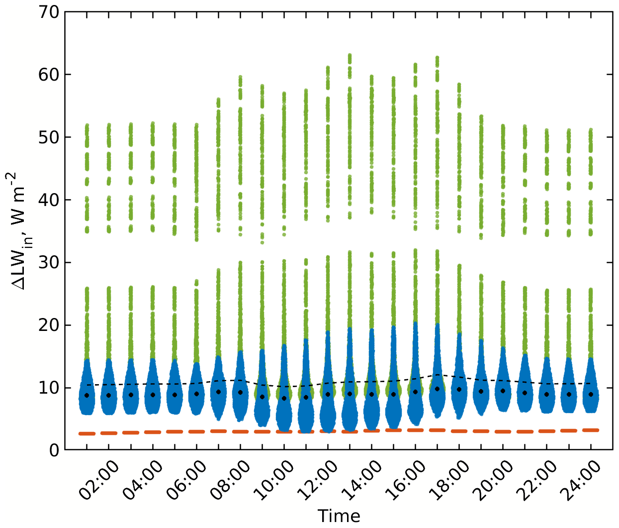
Figure 11Changes in the received LW irradiance within the focus domain of the simple urban configuration when considering tree thermal emissions (RTM_05) compared to the RTM_04. Violin, mean, and median colours are used in the same way as those in Fig. 5.
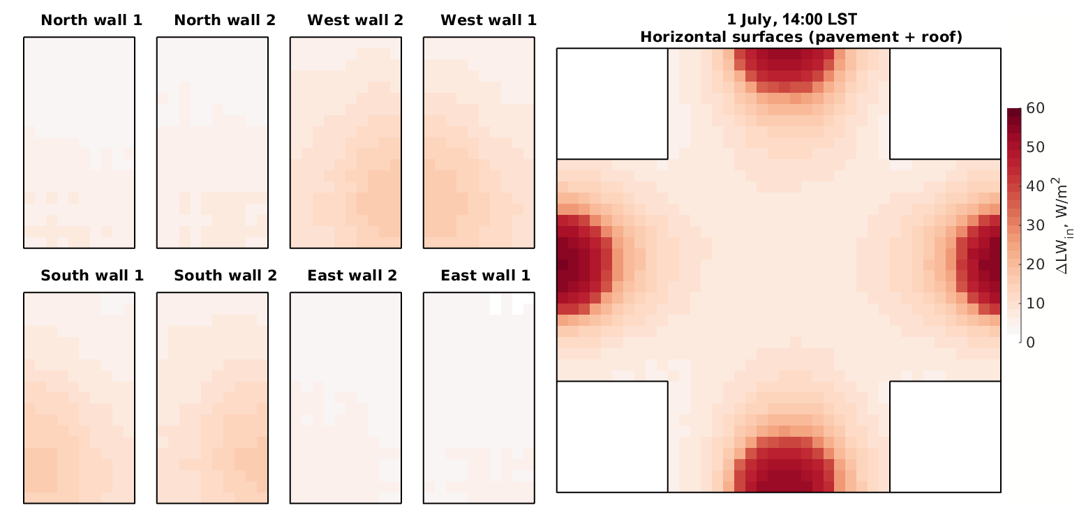
Figure 12Changes in the received LW radiation flux within the focus domain of the simple urban configuration when including vegetation interaction with LW radiation (RTM_05) compared to RTM_04. Walls, roofs, and pavements are folded the same way as those in Fig. 6.
Here, surfaces receive more LW emissions compared to the previous case by up to 60 W m−2 (Figs. 11 and 12). This is an indication that the emitted LW radiation from trees is higher than the absorbed, resulting in higher LW radiation received by surfaces. Since surfaces have different view factors to trees, the LW radiation received by the surfaces is affected by the tree-surface relative location (Figs. 11 and 12). Recalling the parameterization of this step in the RTM (Sect. 2.4.6), the leaves' temperature is set to the surrounding air temperature. During daytime, the net incoming radiation under the trees is still lower by 400 W m−2 compared to its surrounding. During nighttime, this situation is reversed. We find about 90 W m−2 more net radiation under the tree compared to the surroundings.
Allowing vegetation interaction with LW radiative transfer modifies the radiation balance in urban areas. Particularly, it increases the outgoing LW radiation due to increasing the LW radiation absorption within vegetation, reflection from surfaces, and emission from surfaces due to its higher temperature compared to RTM_04. This in turn modifies the effective urban parameters which control the RRTMG–RTM coupling.
4.1.6 Single reflection (RTM_06)
Figure 13 gives the changes in the SW and LW received radiation due to considering a single reflection in the RTM. The figure shows that all surfaces receive radiation from the reflected radiation from other surfaces, which depends on the surface albedo and surface emissivity except the roof surfaces that do not have a view to other surfaces. However, how much additional radiation a surface receives by reflection from another surface depends on their mutual VF as well as on the amount of reflected radiation. For such a simple and regular configuration the variability of the reflected LW radiation is low among surfaces. Therefore, the VFs are predominating. However, this is not the case in SW radiation. Surfaces near unshaded surfaces receive up to 60 W m−2 reflected SW radiation at 14:00 UTC while other surfaces receive less (Fig. 14).
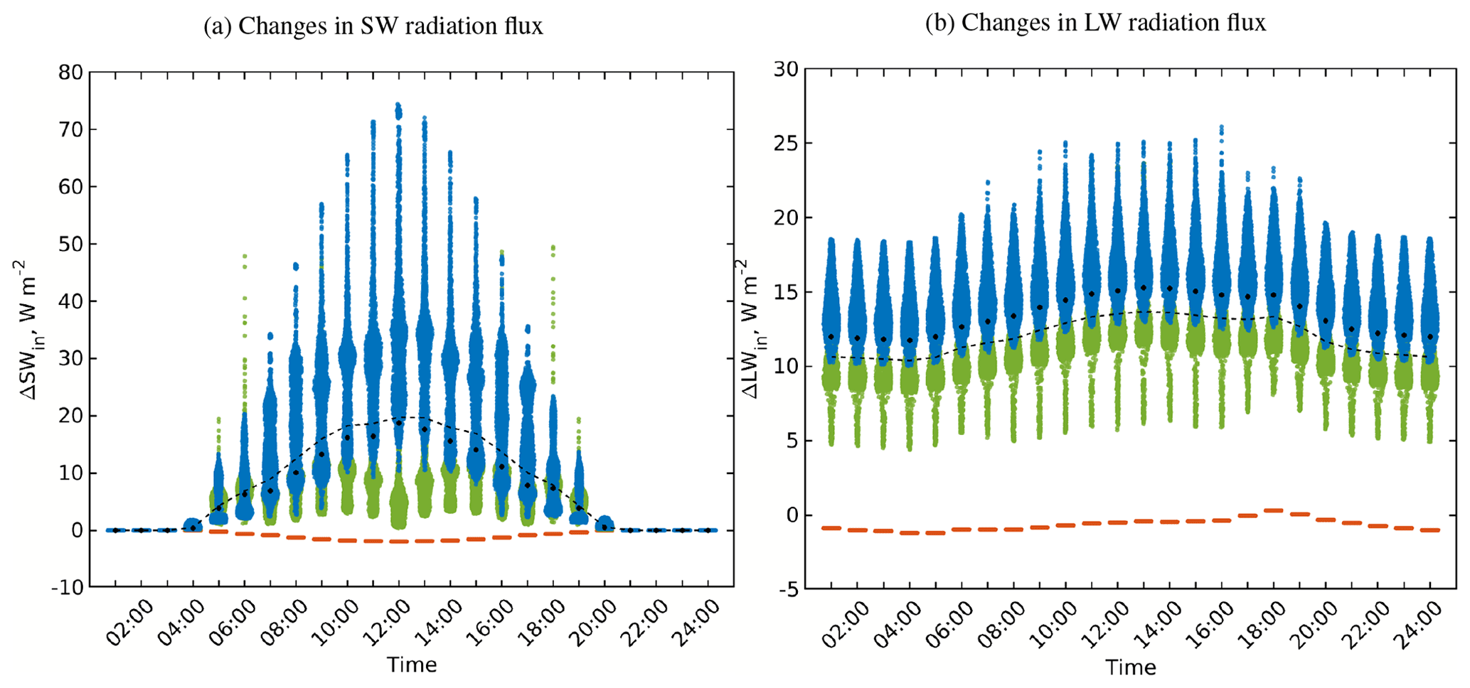
Figure 13Changes in the received SW and LW irradiance within the focus domain of the simple urban configuration when considering one reflection (RTM_06) compared to RTM_05. Violin, mean, and median colours are used in the same way as those in Fig. 5.
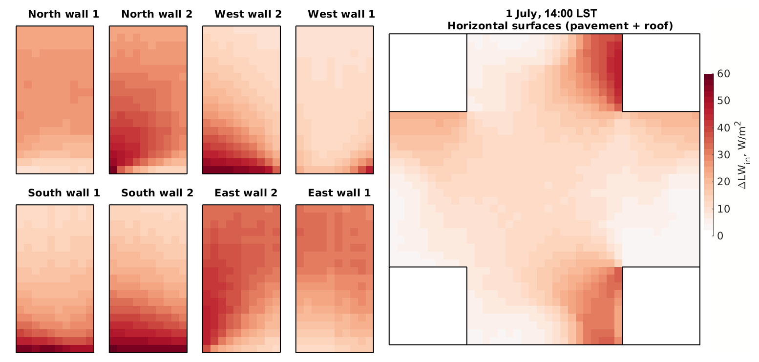
Figure 14Changes in the received SW radiation flux within the focus domain of the simple urban configuration when considering one reflection (RTM_06) compared to RTM_05. Walls, roofs, and pavements are folded the same way as those in Fig. 6.
The RTM in PALM is designed in such a way that surfaces absorb all the received reflected radiation after the last reflection step which in the case of RTM_06 is one reflection. In other words, surfaces do not reflect part of the received radiation from reflection. For this reason, the consideration of only a single reflection is not enough to account for realistic simulations especially for surfaces with low emissivity or high albedo.
4.1.7 Vegetation interaction with reflected radiation (RTM_07)
Since the change in the incoming SW radiation from the RRTMG radiation model is negligible in this step (Fig. 3a), all surfaces receive up to 1.2 W m−2 less reflected SW radiation due to vegetation compared to the previous case. Interestingly, small positive values in ΔLW less than 0.6 W m−2 are observed in particular during nighttime although negative values are expected. Some surfaces may receive slightly higher reflected LW radiation when the RTM includes the vegetation interaction with reflected radiation. Meanwhile, the incoming LW radiation from the RRTMG radiation model is slightly less than in the previous case (RTM_06) (Fig. 3b). This behaviour is attributed to the variability of the vegetation LW emission (see Sect. 2.4.6), which is calculated based on the instantaneous local air temperature. For instance, the spatial distribution of the received LW radiation for all surfaces in the focus domain, not shown here, shows that some surfaces receive slightly higher LW radiation flux compared to other surfaces for this particular time. When the local air temperature changes due to the model dynamics the vegetation LW emission changes as well and the surfaces receive different reflected LW radiation accordingly.
4.1.8 Multiple reflections (RTM_08)
The received SW and LW radiation gained by increasing the reflection steps from a single reflection to four reflections is depicted in Fig. 15. During each reflection step, vegetation absorbs part of the reflected radiation, similar to the previous processes (Sect. 2.4.8). The surfaces which have no mutual view to other surfaces, especially roof surfaces receive no reflected SW radiation. Also, the change in the incoming SW radiation from the RRTMG radiation model is not large enough (Fig. 3a) to change their incident SW irradiance. Nevertheless, these surfaces receive less LW radiation since the incoming LW radiation from the RRTMG radiation model is smaller compared to RTM_07 (Fig. 3b).
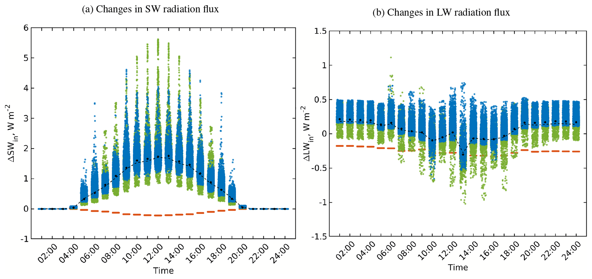
Figure 15Changes in the received SW and LW irradiance within the focus domain of the simple urban configuration when considering multiple reflections (RTM_08) compared to RTM_07. Violin, mean, and median colours are used in the same way as those in Fig. 5.
It is important when performing multiple reflections to monitor the residuals after each reflection step. That is to assure that the absorbed radiation at the last reflection step is small enough so that any further reflections can be ignored. As a matter of fact, reflected radiation flux density has an order of αN for shortwave and (1−ϵ)N for longwave radiation. The SW and LW radiation residuals in the surfaces after four reflection steps are small enough and the reflection process can be safely terminated (figures are not shown to save space).
4.2 Surface radiation flux for the realistic urban configuration
Generally speaking, the changes in the surface radiation flux of the realistic urban configuration when applying SPM show similar behaviour to the simple urban configuration. However, due to the complexity of the building configurations and the heterogeneity of the surface characteristics of the realistic case, these changes are more complex. As a matter of fact, the buildings of the simple configuration have the same height; therefore, the differences of the radiation incident on the roofs result mainly from the RRTMG–RTM coupling. Also, the trees are chosen so that they are shorter than buildings, which may underestimate the their effect.
In this section, we show examples of the changes in the radiation fluxes for the realistic case and we highlight the differences compared to the simple case.

Figure 16The daily course of (a) incoming shortwave and (b) incoming longwave radiation fluxes for the top of urban layer of the realistic urban configuration at 52∘ N on 1 July.
First, the incoming SW and LW radiation fluxes from the RRTMG radiation model, shown in Fig. 16, vary more with each SPM step as a result of RRTMG–RTM coupling than in the simple case. In fact, both the effective urban characteristics (albedo, emissivity, and temperature) and the atmospheric properties (i.e. air temperature, humidity, pressure, etc.), which are the inputs to the RRTMG radiation model, change more in the realistic case than the simple case. This represents an implicit effect of the radiation parameterization on the simulation of a realistic urban configuration.
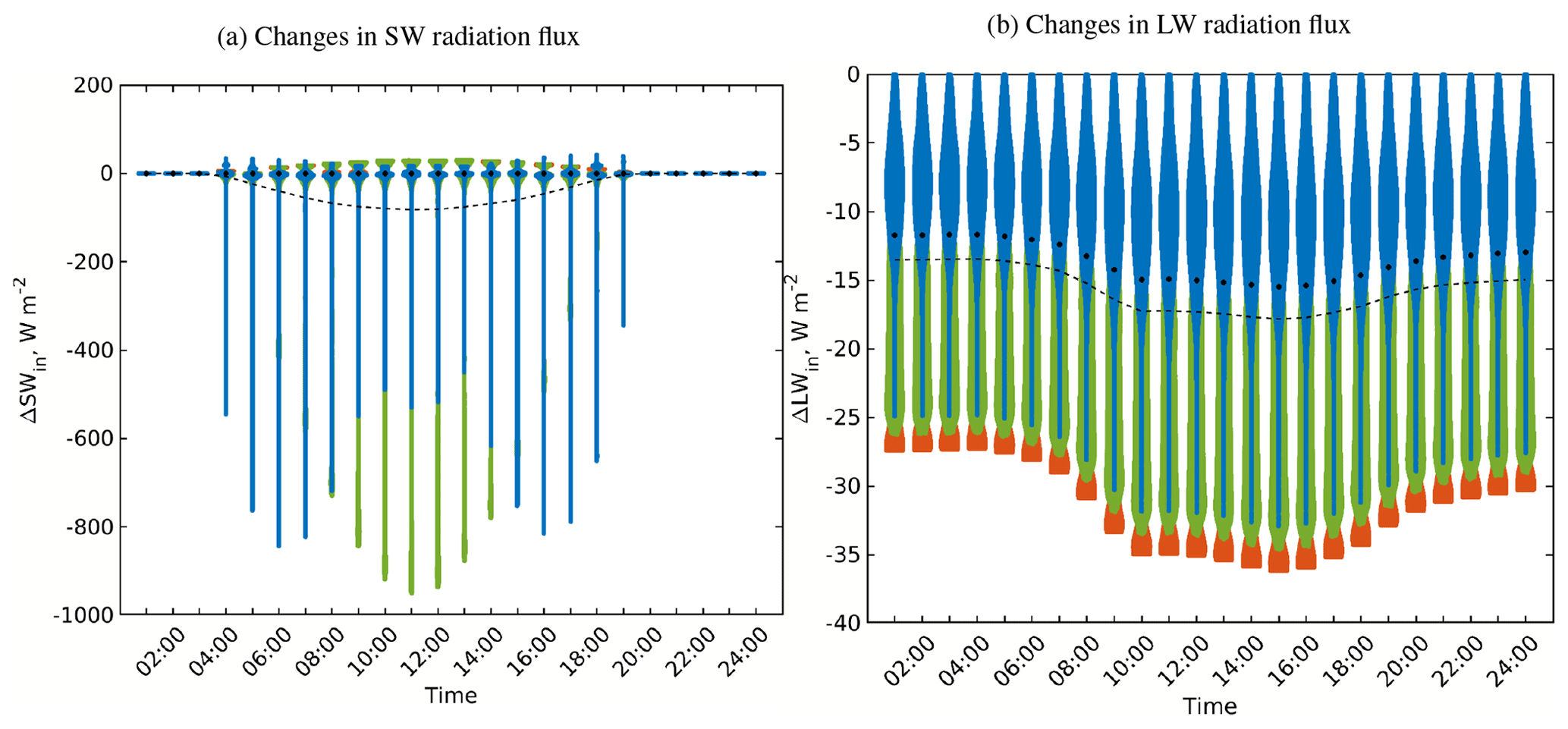
Figure 17Changes in the received SW and LW irradiance for the surfaces of the realistic urban configuration when considering vegetation interaction with SW solar radiation (RTM_03). Violin, mean, and median colours are used in the same way as those in Fig. 5.
Secondly, the magnitude of the changes in the radiation fluxes due to considering a specific RTP is higher than the changes in the simple urban configuration. This can be attributed to the complexity of the urban configurations and its surface characteristics. Also, the variability in the incoming radiation from the RRTMG radiation model to the urban domain contributes to these changes. For instance, including the vegetation interaction with SW radiative transfer (RTM_03) decreases the received SW radiation of the surfaces located in the view of the vegetation (Fig. 17a). Since the vegetation in the realistic configuration is heterogeneous and denser than in the simple case, its effect is much higher (Fig. 18). Consequently, the urban domain air cools down compared to the previous RTM, and therefore the incoming LW radiation is lower (Fig. 17b).
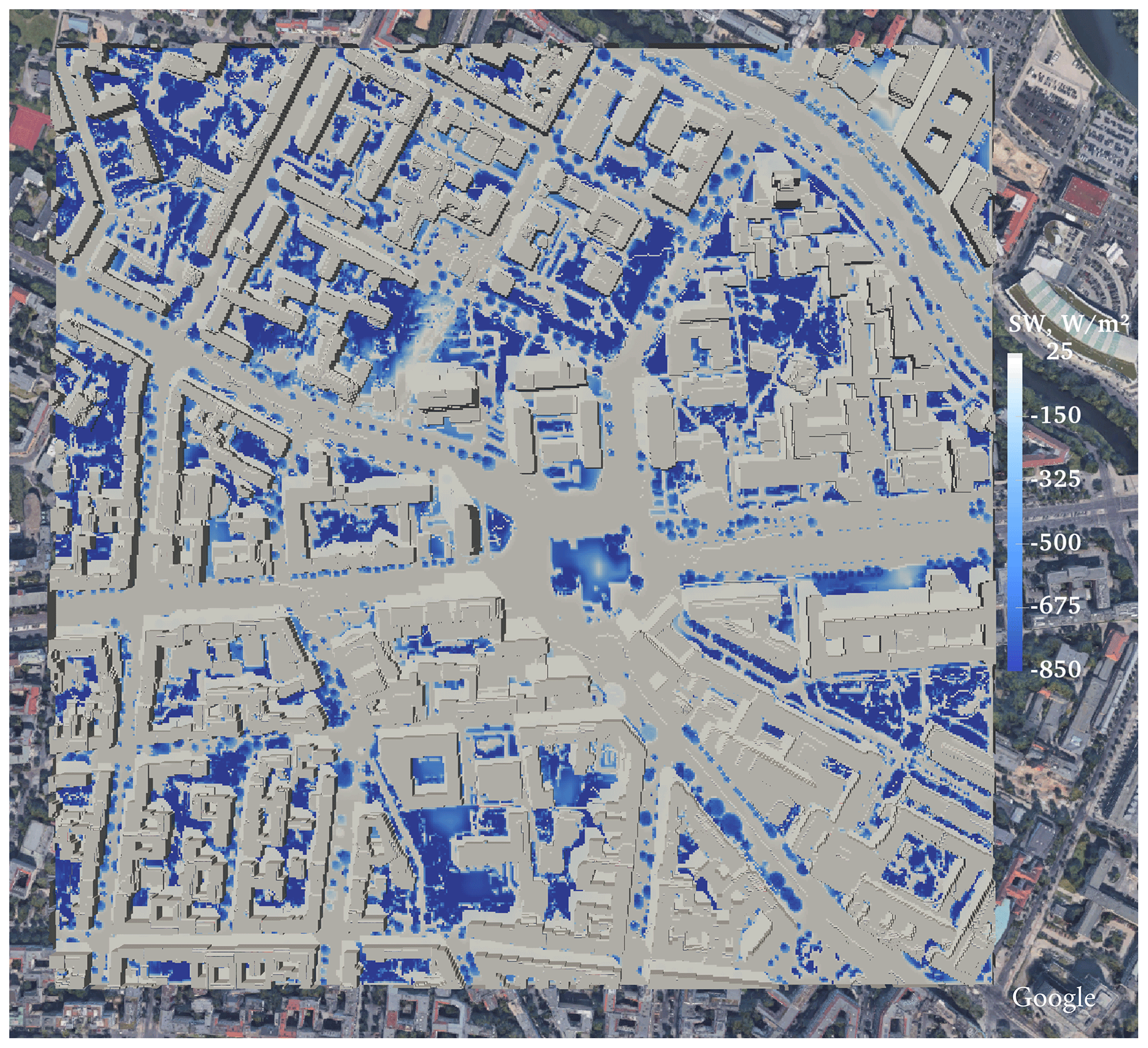
Figure 18Changes in the received SW radiation flux for the realistic urban configuration at 10:00 LST due to including the vegetation interaction with the SW radiative transfer (RTM_03). The copyright for the underlying satellite image is held by © GeoBasis-DE/BKG 2009, Google 2009.
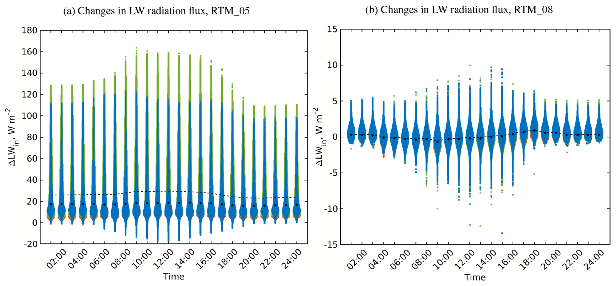
Figure 19Changes in the received LW irradiance for the surfaces of the realistic urban configuration when considering (a) the vegetation interaction with LW radiation (RTM_05) and (b) the multiple reflections (RTM_08). Violin, mean, and median colours are used in the same way as those in Fig. 5.
Thirdly, the effect of the RTPs related to the vegetation interaction with LW radiation transfer is more pronounced and even more complex compared to the simple case. As described in Sect. 2.4.6 and 2.4.8, the LW emission from vegetation is based on the leaves' temperature which is set to the surrounding air temperature. In such complex geometry, the air temperature varies with the flow dynamics, especially in simulations based on LES, and hence the vegetation thermal emissions. Also, the absorbed LW radiation by vegetation is directly released to the air which further modifies the temperature field in the domain. These vegetation-related processes implicitly modify the thermal emissions from urban surfaces (walls, pavements, etc.) by modifying the surface temperature of these surfaces. This in turn changes the received LW radiation from surface thermal emission. Ultimately, the total received LW irradiance for a surface is the combination between the received LW radiation from the sky and from the surface thermal emissions after the partial absorption in the vegetation boxes and the thermal emission from the vegetation boxes themselves. For example, Fig. 19 shows two examples of the changes in the received LW radiation flux for the realistic case. Figure 19a gives the changes in the received LW radiation flux due to including the thermal emissions from vegetation. Although most of the surfaces receive higher LW irradiance, due to vegetation emissions, some surfaces receive slightly less LW irradiance. For those surfaces, the absorbed LW radiation in vegetation is higher than that received from the vegetation thermal emissions. In Fig. 19b, the changes in LW irradiance due to including multiple reflections are depicted. The variability in the temperature field which drives the vegetation thermal emissions affects the total LW radiation flux received by each surface. The spacial distributions of these changes are plotted in Fig. 20.
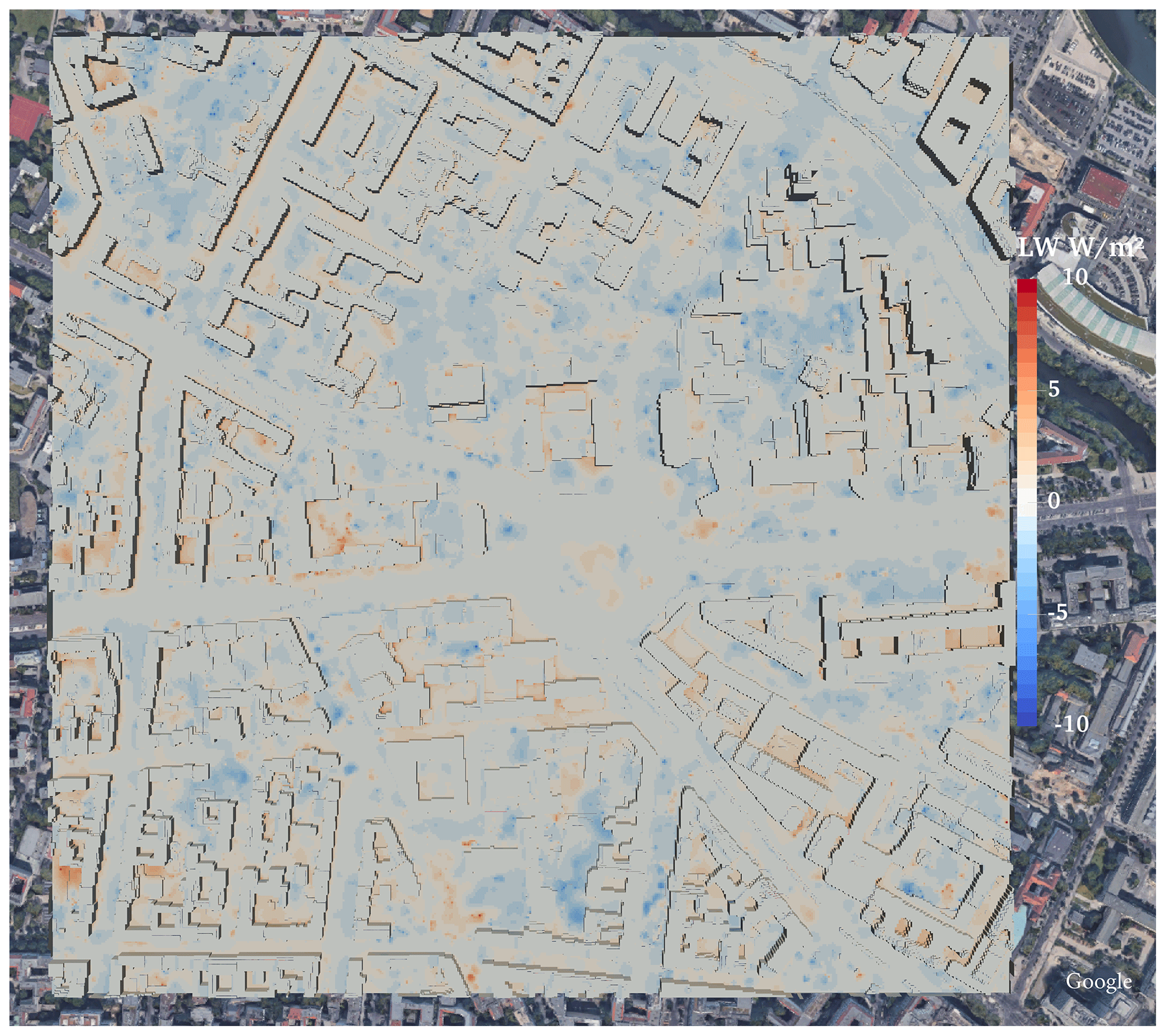
Figure 20Changes in the received LW radiation flux for the realistic urban configuration at 12:00 LST due to including multiple reflections (RTM_08). The copyright for the underlying satellite image is held by © GeoBasis-DE/BKG 2009, Google 2009.
4.3 Wind flow properties
The general effect of the thermally driven flow within the UCL has been discussed in many previous studies (e.g. Qu et al., 2012; Park et al., 2012; Xie et al., 2005). However, we focus here on the dynamic and thermal flow properties' response to the different combinations of RTPs rather than addressing the radiation as a bulk process. We first show the effect of RTPs on the average vertical profiles of the flow properties and then we use the quantification measures described in Sect. 3.3.2 to quantitatively monitor these effects.
Each parameterization step of SPM yields RTM, and hence UCM, with varying combinations of radiative interaction processes (Sect. 2.4). The different RTM produce different radiation budgets for surfaces, as discussed in Sect. 4.1 and 4.2. The heated surfaces add buoyancy force to the flow in addition to the inertial and the mechanical shear forces. The interaction of these forces alters the structure of the recirculating flow within street canyons and above building roofs generating different flow patterns. Presumably, this affects all exchange processes within the urban boundary layer.
Since the flow in each simulation responds to different combinations of RTPs, results are presented in a normalized form. The average building height, H, is used as the canopy height to characterize the length scale. The velocity scale, Ur, is set to be the time-varying horizontally averaged wind speed at the atmospheric boundary-layer depth of case RTM_08 (the full RTM, Sect. 2.4.9). The horizontally averaged potential temperature of RTM_08 at the same height is utilized as a comparison temperature. Both the horizontal wind speed () and the turbulent quantities (turbulent kinetic energy, e, and vertical turbulent flux of potential temperature, ) are normalized using these characteristic scales.
4.3.1 Mean profiles
During the simulations, instantaneous flow properties such as wind velocity components (u, v, w) and potential temperature (θ) are calculated every time step. After the spin-up time, the averaged values as well as the turbulent fluctuations (as deviations from the averaged values) are calculated every 3600 s of the simulated time. The quantities then are horizontally averaged to create horizontally averaged vertical profiles every 1 h. These time-varying horizontally averaged profiles of the flow components represent the changes of these quantities during the diurnal cycle. Figures 21 and 22 show the vertical profiles of the normalized averaged wind speed, the deviation of potential temperature from the near-surface value, and the vertical turbulent flux of potential temperature at 10:00 LST for the simple and the realistic urban geometry, respectively. These flow properties are chosen to represent the wind and scalar statistics.
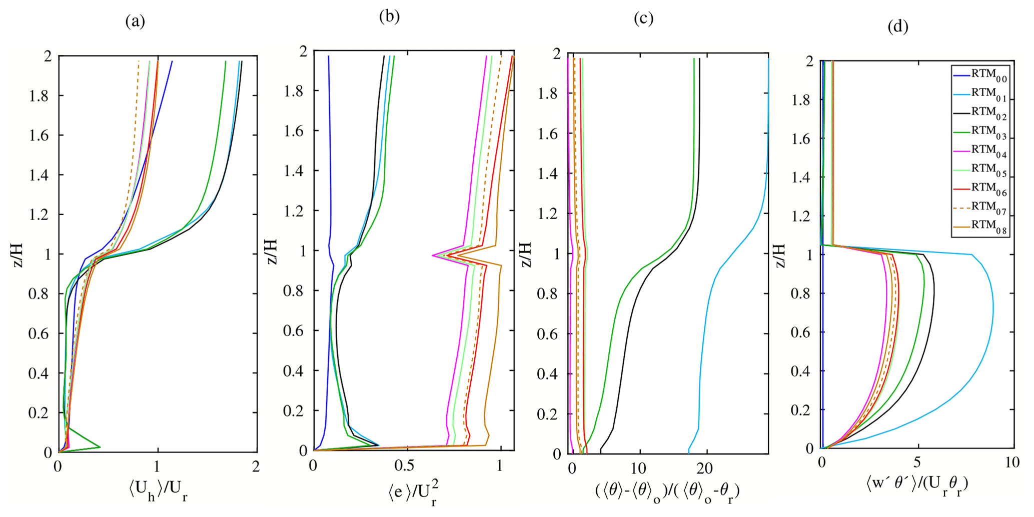
Figure 21Horizontal- and time-averaged (1 h) vertical profiles of the simple urban configuration at 10:00 LST of (a) horizontal wind speed , (b) turbulent kinetic energy 〈e〉, (c) normalized vertical potential temperature 〈θ〉 deviation from the near-surface potential temperature 〈θ0〉, and (d) normalized vertical turbulent flux of potential temperature . Each quantity is normalized by its relevant combination of velocity (Ur), temperature (θr), and height scale (H). The reference velocity and temperature are the respective values at 2H and the height scale is the building height.
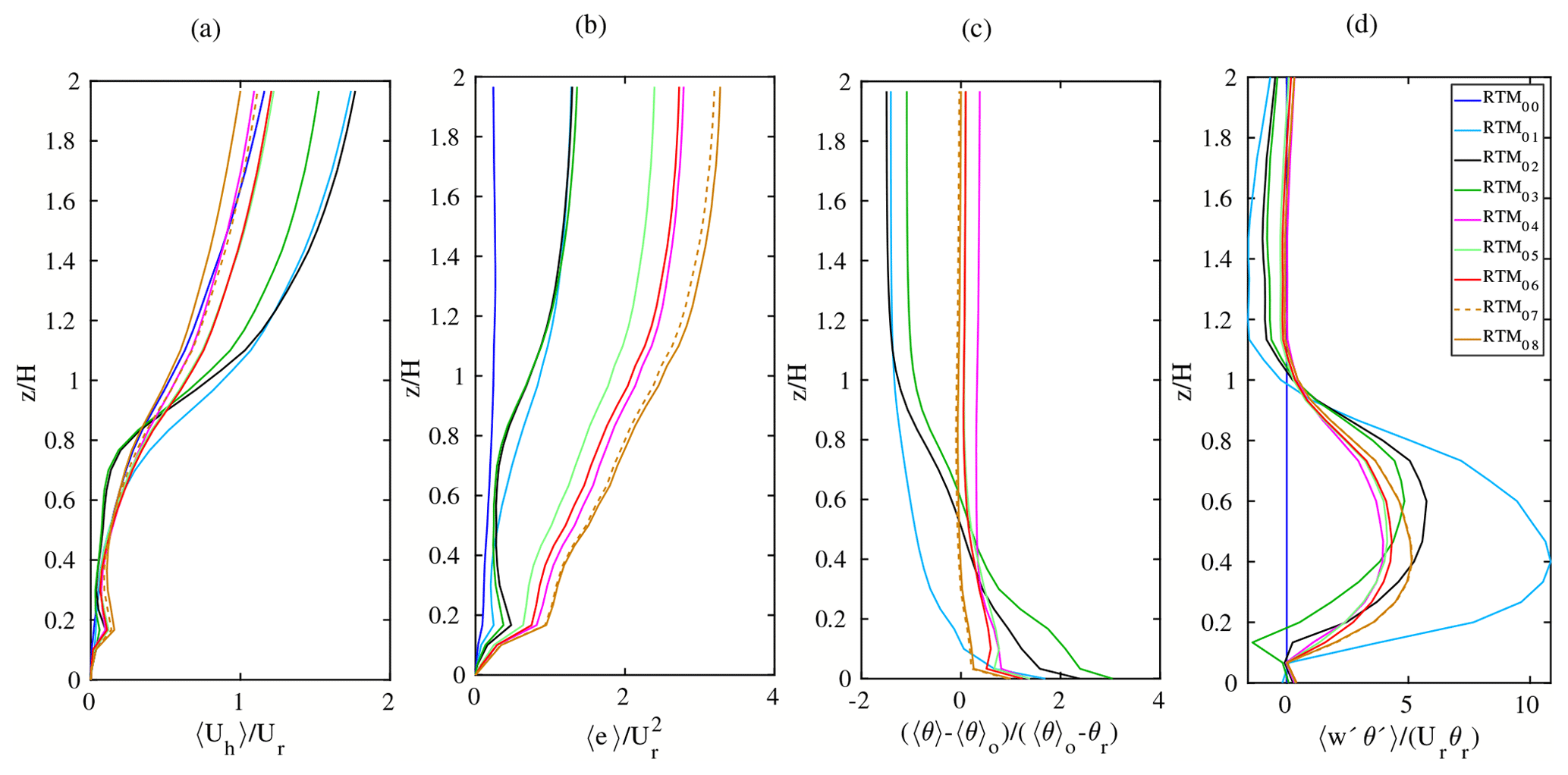
Figure 22Horizontal- and time-averaged (1 h) vertical profiles of the realistic urban configuration at 10:00 LST of (a) horizontal wind speed , (b) turbulent kinetic energy 〈e〉, (c) normalized vertical potential temperature 〈θ〉 deviation from the near-surface potential temperature 〈θ0〉, and (d) normalized vertical turbulent flux of potential temperature . Each quantity is normalized by its relevant combination of velocity (Ur), temperature (θr), and height scale (H). The reference velocity and temperature are the respective values at 2H and the height scale is the mean building height.
Comparing the profile shapes and the vertical gradients reveal that the effect of radiation parameterization on the flow is considerable below and above the street canyons. This is even visible in the simple urban geometry, compared to the realistic case where the horizontal surfaces are distributed at many vertical levels. Three groups of profiles can be identified. The first group is related to the results based on RTM_00 to RTM_03. Basing the PALM only on these RTMs produces high discrepancies in both the wind and the turbulence characteristics compared to RTM_08. The second group includes the profiles based on RTM_04 to RTM_06 which allow surfaces to receive LW irradiance from surfaces and vegetation as well as reflected SW radiation from surfaces. These parameterizations enhance both the wind and the scalar profiles and remarkably adjust the vertical profiles and hence represent the minimum parameterization of radiation interaction in order to produce reasonable vertical profiles of flow properties. The third group includes the profiles based on the last RTMs, i.e. RTM_07 and RTM_08. These parameterizations have subtle effect on the profiles shape and merely serve to fine tune the flow profiles. This finding is not surprising since the change in surface radiation budget due to the additional radiation interaction processes in these RTMs is low, compared to those in the previous RTMs.
4.3.2 Quantitative analysis
The heterogeneity of surfaces with different radiation budgets due to their orientation and surface characteristics creates local flow changes that are not visible in the flow profiles discussed above. Each process ultimately initiates different thermally induced forces which interact with both the shear forces of the flow above the surfaces and the driving forces induced by building corners, creating eddies yielding to the complex three-dimensional flow field. This spatial variability in the flow field arising from using different RTMs is quantified by calculating the root mean square of the relative error vector in the flow properties, nRMSEψ, Eq. (7) and the normalized volumetric flow rate, , Eq. (8), for each particular SPM step, as discussed in Sect. 3.3.2.

Figure 23Box plots of the error measure, nRMSE, for (a) the horizontal wind speed , (b) the vertical wind speed 〈w〉, and (c) the air potential temperature 〈θ〉 for the focus domain of the simple urban configuration. For each parameter, nRMSE is calculated hourly for 1 d (1 July) for each RTM configuration.
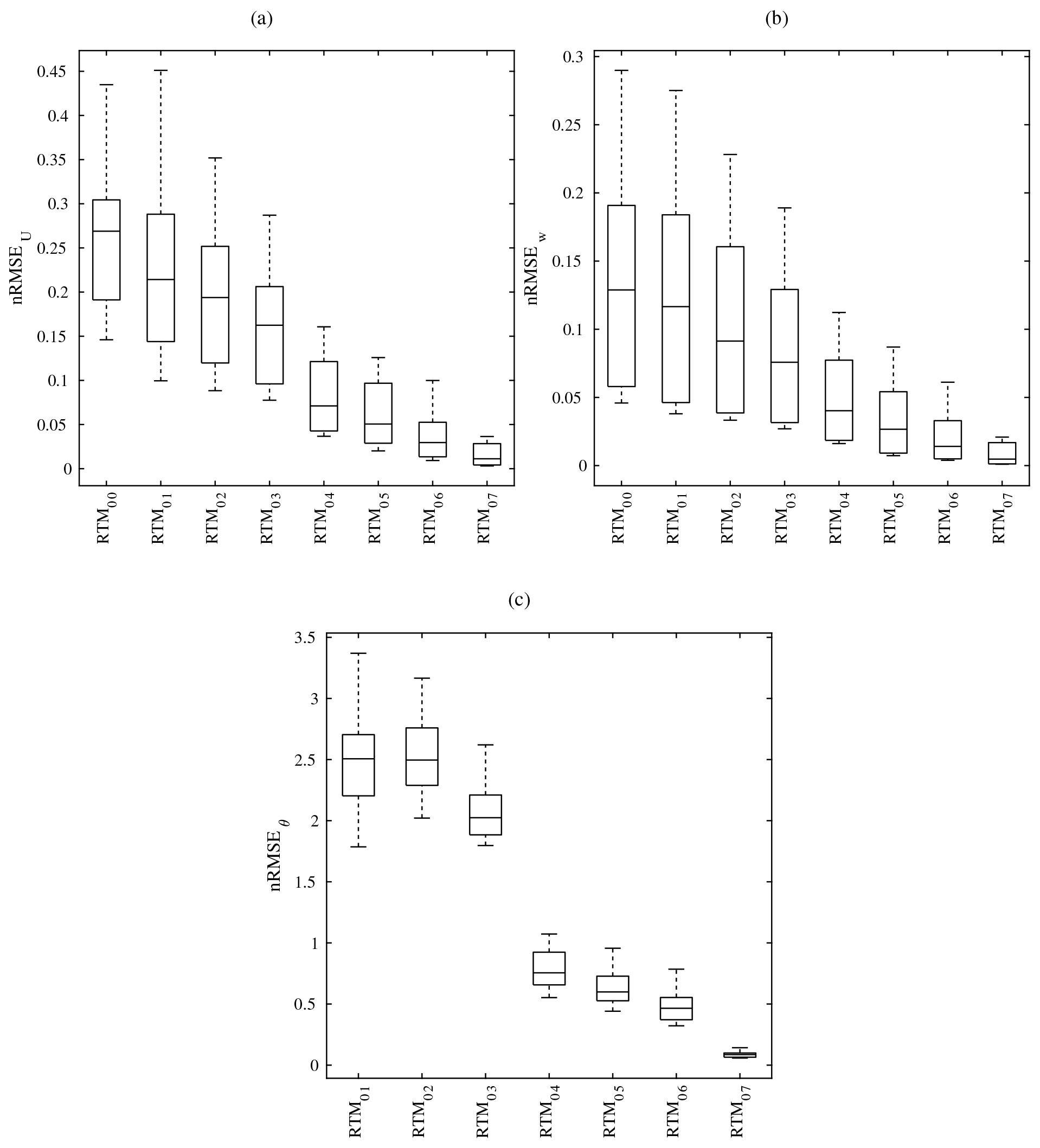
Figure 24Box plots of the normalized root mean square error, nRMSE, for (a) the horizontal wind speed , (b) the normalized vertical wind speed 〈w〉, and (c) the air potential temperature 〈θ〉 for the focus domain of the realistic urban configuration. For each parameter, nRMSE is calculated hourly for 1 d (1 July) for each RTM configuration.
For the relative error measures, the flow properties chosen are the normalized horizontal and vertical wind speed and the air potential temperature. According to these measures, successive incorporation of RTPs results in reduction in nRMSE (Figs. 23 and 24), indicating improvement of solution quality. The results based on RTM_07 are close to the results of RTM_08 throughout the day. For this RTM, nRMSE of horizontal and vertical wind speed are negligible (less than 2 %) in both the simple (Fig. 23a and b) and the realistic (Fig. 24a and b) urban configurations. Also nRMSE values of the air temperature are very small (less than 0.2 K). Accordingly, including this RTP in the RTM seems to have a marginal effect on the flow properties even in the realistic urban configurations. The results based on RTM_04 to RTM_06 are of good quality. For wind speed, nRMSE values are mostly less than 5 % for both urban configurations. Compared to the RTM_08 results, the variability in nRMSE values is not high throughout the day, yet higher in the daytime (Figs. 23 and 24). On the other hand, RTM_00 to RTM_03 produce low-quality results, based on the calculated nRMSE (Fig. 23 and 24). The discrepancies induced by omitting the processes covered in RTM_01 to RTM_03 in the velocity field are high and may essentially impact all velocity-related parameters, such as wall shear stress and others.
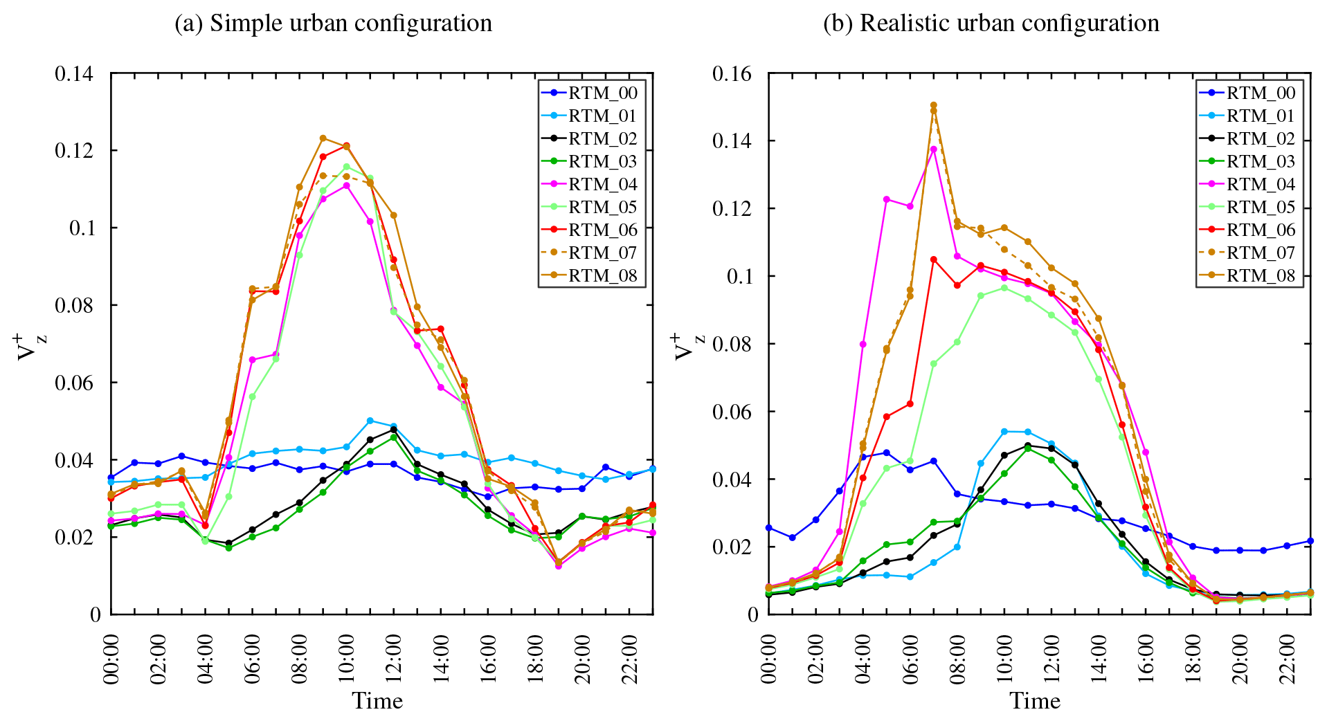
Figure 25The normalized volumetric flow rate for (a) the realistic and (b) the simple urban configuration for all SPM steps.
For the normalized volumetric flow rate, is calculated for a complete diurnal cycle at a horizontal plan set at a height . The characteristic velocity is set to the velocity scale Ur at the corresponding time. Comparing for all cases clearly shows that including different RTPs alters the air volume flow through the corresponding plane (Fig. 25). It indicates that the rotation of air mass in the streets has been changed as a result of the interaction between the mechanically and the thermally induced forces. The air mass rotation varies during the day as the thermally induced forces change with time, and according to the RTM used. The results for both the simple (Fig. 25a) and the realistic (Fig. 25b) urban configurations confirm the results of the relative error measures. The values based on RTM_00 to RTM_03 are quite low compared to the those based on RTM_08, while the values based on RTM_04 to RTM_06 are relatively close to the values based on RTM_08. The effect of multiple reflections, i.e. RTM_07 on the values, is quite small, compared to those of RTM_08.
4.3.3 Overall effect
Based on the above discussion, the effect of using different RTMs on the flow properties may be summarized as follows:
-
In combination, our analysis confirms the hypothesis that using different combinations of RTPs considerably alters the flow properties (scalar and turbulence) within the urban canopy layer.
-
Each RTP affects the flow field differently, based on its contribution to the surface radiation budget. Some processes have primary effects on the flow, while other processes have only secondary effects.
-
Considering the SW interaction with buildings and vegetation (shadow casting) only in the RTM is not recommended, especially during the day, and may produce high discrepancies in the flow properties and all its related parameters.
-
The processes of buildings and vegetation interaction with LW transfer, such as thermal emissions, are essential in RTM to assure acceptable quality of the model results.
-
Including SW and LW radiation reflection process in RTM affects the flow properties. It is important to include both SW and LW reflection in the RTM to produce high-quality model results.
-
The changes in the radiation budget of surfaces due to considering vegetation interaction to reflected irradiance and/or multiple reflections in the RTM are not strong enough to create a considerable effect on the flow properties.
-
Generally, the effects of RTPs depend on the time of the simulation. For example, processes related to the interaction with SW radiation obviously are only important during the day.
-
The change in the flow properties due to the sophistication of RTM is not limited to the flow between buildings, but its influence extends above street canyons.
4.4 Computational aspects
As pointed out in Sect. 1, computational resources, i.e. computation time (CPU time) and memory space, may pose hard constraints to include all RTPs into the RTM. The demand for these resources may vary during the simulation, depending on the design of the RTM. For instance, during the model initialization, the RTM needs a considerable amount of computational resources to perform the ray tracing to calculate the geometrical fields related to the RTM, such as SVFs, SV, and CSF. These fields are usually not fully aggregated or stored in size-optimized arrays in the initialization phase. Also the model needs other helping fields to calculate the main fields, which are deallocated after the initialization. During the time integration (time-stepping) phase, RTM uses less computational resources, compared to the initialization, because it allocates only the required fields, and, since the geometry is fixed, the geometrical fields are not recalculated. The resources required for the restart and the post-processing depend on the model steering and usually are not as demanding as in the initialization phase. We limit the analysis of the computational resources here to the time-stepping phase because the other two parts are needed only once during the simulation and may vary depending on the discretization scheme and the ray-tracing algorithm.
Table 2 compares the essential computational resources needed for the RTMs of the SPM. These RTMs can be divided according to its computational resources demand into two groups. The first group, RTM_00 to RTM_03, requires low computational resources because these RTMs consider only the RTPs related to the atmosphere–surface interaction. The computational resources in these processes usually grow in the order of the number of surfaces and plant canopy boxes (first order), since there is no mutual interaction between the surfaces and the plant canopy boxes. The second group, i.e. RTM_04 to RTM_08, needs considerable amount of computational resources since RTMs in this group additionally account for the RTPs related to surface-to-surface radiative interaction as well as vegetation interaction with LW radiation. These processes, however, increase the computational resources for a domain size n×n by an order of magnitude O(n5) or O(n3), depending on the discretization scheme.
Table 2The computational resources requirement of the RTMs used in the SPM for the realistic urban configuration. The CPU time is given relative to the CPU time of RTM_08 (3422 min, excluding the initialization, restart, and post-processing phases). Note that the RTM requires <5 % of total runtime of the model run with RTM_08. The memory space is given for the essential fields only.
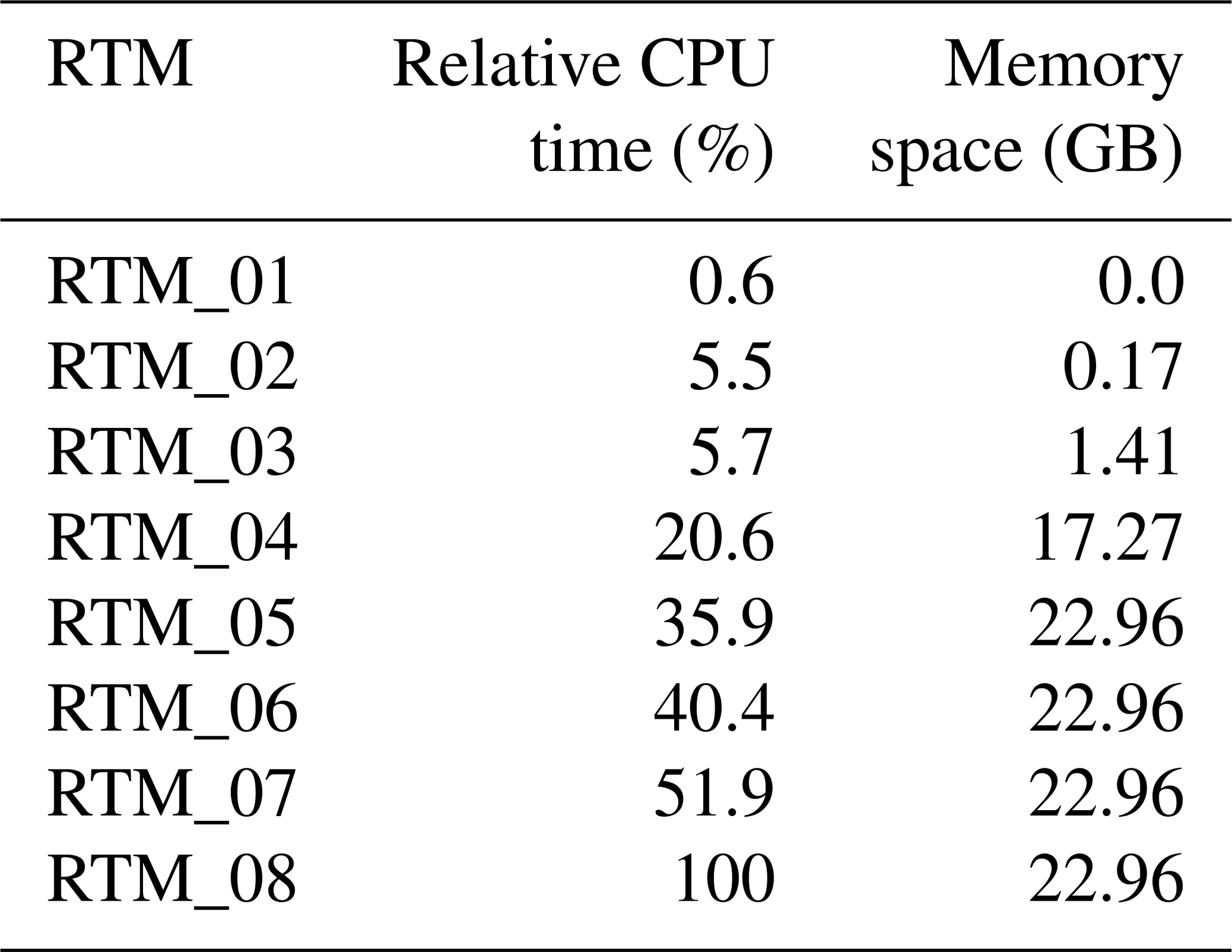
As Table 2 shows, there is no additional memory demand after the RTM_05 because all the essential fields are already calculated. This suggests that, from the memory point of view, it is recommended to use the full RTM, i.e. RTM_08 when all the RTPs of the RTM_05 are, at least, needed because all other RTPs included in the RTM_08 come with no further memory space demand. The table shows also that there is a considerable steady increase in the CPU time starting from RTM_04. This is due to the time needed for MPI data exchange for each time step for the surface-to-surface and plant-canopy-box-related RTPs. However, this may not represent an issue for the whole model CPU time since the CPU time demand for RTM is small for a well-designed and optimized models (<5 %). Nevertheless, the RTM may implicitly increase the CPU time by modifying the turbulent flow, due to the buoyancy force, which results in a decreased time step.
4.5 Limitations and outlook
The generalizability of the results of this study is subject to certain limitations. For instance, all the simulations were performed on a typical urban scenario during a summer day with clear-sky conditions. Neither clouds nor rain were considered in this study. The effect of RTPs, especially those controlling SW radiation, will change for other than clear-sky conditions. However, clear-sky conditions are usually used for urban-specific applications. Since the study was based on the model system of PALM, it was not possible to consider the effect of absorption, emission, and scattering of radiation due to air constituents (fog, pollutants, etc.). Also, all surfaces are assumed to be Lambertian reflectors; therefore, directional reflection is not considered. Another limitation is the dependency of the results on the surface properties (albedo, emissivity, roughness, and skin layer thermal conductivity) and parameters of building and pavement materials (volumetric heat capacity and thermal conductivity). Although we made sure to use typical surface properties in the two urban configurations, simulations for domains with different surface properties may show different results.
The current study focuses on the flow changes within the urban domain. A further study could assess the performance of the RTMs using simulations with fixed meteorological conditions. In this way, the secondary effect of each RTM caused by the variation of meteorological conditions will be eliminated. This will keep the focus on the pure radiative transfer processes. Further research could also be conducted to determine the influence of using different radiation transfer processes on the atmospheric boundary-layer-scale structure and its impact on turbulent exchange at the canopy–atmosphere interface. Further studies need to be carried out in order to explore canopy exchange of scalars (e.g. pollutant dispersion). These suggested studies would make use of the output of the measurement campaign which was completed in the first phase of the [UC2] project to evaluate the PALM model and the TURBAN project (https://project-turban.eu/news.html, last access: 27 December 2021) which provides filed observations which should help to validate details of the turbulent flow in the street canyons.
The purpose of the current study is to determine how much detail should be included to parameterize the radiative transfer in UCMs. A generic parameterization method is used to quantify the effect of including the main RTPs into the RTM of an UCM in a stepwise manner. These processes include interaction of urban elements (buildings and trees) with both the incoming SW radiation (e.g. shadow casting) and LW radiation (e.g. thermal emission and absorption) as well as radiation reflections among urban elements. The results show that although these processes contribute differently to the surface radiation budget, they are necessary to accurately estimate the radiation budget of urban surfaces.
Although this study does not engage with validating the RTM, it highlights the main major RTPs which greatly affect the ultimate surface radiation budget. For instance, surface interaction with the incoming SW and LW radiation from the sky is greatly adjusted by calculating the proper SVFs, and hence the received radiation from sky to surfaces is correctly added to the radiation budget. Also, and as expected, the vegetation interaction with the incoming SW radiation from the sky has a great effect on the surfaces located in their view area. The radiation budget is greatly adjusted by estimating the vegetation shadows due to vegetation. Additionally, receiving LW irradiance from urban surfaces constitutes a major part of the received LW radiation budget. Similarly, the vegetation interaction with LW irradiance process affects the radiation budget of the surfaces located in their view by partially absorbing the LW irradiance from the sky and emitting LW irradiance from the biomass.
The study shows also that receiving irradiance from the reflected radiation (SW and LW) provides considerable radiation to the radiation budget of surfaces, especially to those located in the shadow. Most of the received radiation from reflections is received in the first reflection; however, multiple reflections are still needed to reduce the residuals. It is confirmed that using finite number of reflections is adequate to parameterize radiation reflections since radiation residuals decrease quickly with increasing the number of reflections. Nonetheless, the number of reflections should be chosen based on the surface properties (albedo and emissivity). Vegetation interaction with reflected irradiance has a minor effect on the radiation budget.
The flow field properties (scalar and turbulent) react to the type of the RTM used in the simulation. The flow field is shaped by the interaction between the inertia, mechanical shear, and buoyancy forces. The latter is mainly controlled by the RTPs considered in the RTM. The study identified three categories of RTMs, when compared to the full RTM 3.0, i.e. RTM_08. The first category (RTM_00 to RTM_03) produces low-quality model results. The second category (RTM_04 to RTM_06) gives acceptable model results, based on the quantification measures. Omission of any RTP in these RTMs may lead to considerable uncertainties in the model predictions. The third category (RTM_07) produces high-quality model results. Generally, RTPs modify the vertical distribution of turbulent momentum flux and control the exchange of momentum and scalars. As presented in Sect. 1, this is an essential feature especially when designing/evaluating urban climate application studies, such as pollutant dispersion and outdoor comfort in urban areas.
The study highlights the implicit effect of each RTP on the surface radiation budget and the flow field by altering the incoming radiation fluxes from sky, due to the coupling of the RTM with the radiation model.
| LAD | Leaf area density |
| LES | Large eddy simulation |
| LW | Longwave |
| MPI | Message Passing Interface |
| PALM | Parallelized Large-eddy Simulation Model |
| RANS | Reynolds-averaged Navier–Stokes equations |
| RRTMG | Rapid Radiative Transfer Model for Global models |
| RTM | Radiative Transfer Model |
| RTP | Radiative transfer process |
| SPM | Stepwise parameterization method |
| SVF | Sky-view factor |
| SW | Shortwave |
| UCM | Urban climate model |
| UCL | Urban canopy layer |
| VF | View factor |
The PALM model system is distributed under the GNU General Public License v3 (http://www.gnu.org/copyleft/gpl.html, last access: 27 December 2021). The model source, documentation, user manual, and online tutorial are freely available and can be downloaded from http://palm-model.org (last access: 27 December 2021). Version 6.0 of PALM, which is used for this study, is available via https://doi.org/10.25835/0041607 (Maronga, 2019). This version is based on the Apache Subversion (SVN) revision no. r3668. The SPM is freely available upon a written request to the corresponding author.
The model output data that have been presented in this paper as well as the model driver data are available via https://doi.org/10.5281/zenodo.3934874 (Salim, 2020).
MHS participated in the design of the study, carried out the numerical experiments, analysed the data, and drafted the manuscript; SS participated in the design of the study and in the analysis of the results, and critically revised the manuscript; JR and PK designed the original RTM and revised the study. BM revised the manuscript and coordinated the development of the PALM 6.0 model system. FKS and MS supported the model implementations and the inputs for the test cases and revised the manuscript. CS coordinated the study and revised the manuscript. All authors have read and approved the manuscript for publication.
The contact author has declared that neither they nor their co-authors have any competing interests.
Publisher’s note: Copernicus Publications remains neutral with regard to jurisdictional claims in published maps and institutional affiliations.
This study is funded by the German Federal Ministry of Education and Research (BMBF) under grant no. 01LP1601A within the framework of Research for Sustainable Development (FONA; http://www.fona.de, last access: 27 December 2021), which is greatly acknowledged. The German Aerospace Centre (DLR) Project Management provided the input data for the realistic urban configuration. Simulations have been performed at the supercomputers of the North-German Supercomputing Alliance (HLRN), which is gratefully acknowledged. The co-authors, Jaroslav Resler and Pavel Krč, were supported by the project CZ.07.1.02/0.0/0.0/16_040/0000383 UrbiPragensi – Urbanization of weather forecast, air quality prediction and climate scenarios for Prague under the programme OP PPR “Prague – Growth Pole of the Czech Republic” which is co-financed by the EU. Their financial support was also provided by Norway Grants and the Technology Agency of the Czech Republic “Turbulent-resolving urban modelling of air quality and thermal comfort” project (TURBAN, project no. TO01000219, https://www.project-turban.eu, last access: 30 December 2021).
This research has been supported by the Federal Ministry of Education and Research (Germany) (grant no. 01LP1601A), the European structural and investment funds (grant no. CZ.07.1.02/0.0/0.0/16_040/0000383), Norway Grants, and the Technology Agency of the Czech Republic “Turbulent-resolving urban modelling of air quality and thermal comfort” project (TURBAN, project no. TO01000219).
This paper was edited by Gerd A. Folberth and reviewed by two anonymous referees.
Arakawa, A. and Lamb, V. R.: Computational Design of the Basic Dynamical Processes of the UCLA General Circulation Model, in: Methods in Computational Physics: Advances in Research and Applications, Elsevier, Los Angeles, California, USA,, 173–265, https://doi.org/10.1016/b978-0-12-460817-7.50009-4, 1977. a
Archambeau, F., Méchitoua, N., and Sakiz, M.: Code Saturne: A Finite Volume Code for the computation of turbulent incompressible flows – Industrial Applications, International Journal on Finite Volumes, 1, Institut de Mathématiques de Marseille, Aix-Marseille Université, France, available at: https://hal.archives-ouvertes.fr/hal-01115371 (last access: 27 December 2021), 2004. a, b, c
Bottillo, S., Vollaro, A. D. L., Galli, G., and Vallati, A.: CFD modeling of the impact of solar radiation in a tridimensional urban canyon at different wind conditions, Sol. Energy, 102, 212–222, 2014. a, b
Clough, S., Shephard, M., Mlawer, E., Delamere, J., Iacono, M., Cady-Pereira, K., Boukabara, S., and Brown, P.: Atmospheric radiative transfer modeling: a summary of the AER codes, J. Quant. Spectrosc. Ra., 91, 233–244, 2005. a
Crank, P. J., Sailor, D. J., Ban-Weiss, G., and Taleghani, M.: Evaluating the ENVI-met microscale model for suitability in analysis of targeted urban heat mitigation strategies, Urban Climate, 26, 188–197, https://doi.org/10.1016/j.uclim.2018.09.002, 2018. a
Dai, Y., Zeng, X., Dickinson, R. E., Baker, I., Bonan, G. B., Bosilovich, M. G., Denning, A. S., Dirmeyer, P. A., Houser, P. R., Niu, G., Oleson, K. W., Schlosser, C. A., and Yang, Z.: The common land model, B. Am. Meteorol. Soc., 84, 1013–1024, 2003. a
Dimitrova, R., Sini, J.-F., Richards, K., Schatzmann, M., Weeks, M., García, E. P., and Borrego, C.: Influence of thermal effects on the wind field within the urban environment, Bound.-Lay. Meteorol., 131, 223–243, 2009. a, b
Eichhorn, J. and Kniffka, A.: The numerical flow model MISKAM: State of development and evaluation of the basic version, Meteorol. Z., 19, 81–90, 2010. a
Erell, E.: The Application of Urban Climate Research in the Design of Cities, Advances in Building Energy Research, 2, 95–121, https://doi.org/10.3763/aber.2008.0204, 2008. a
Franke, J., Sturm, M., and Kalmbach, C.: Validation of OpenFOAM 1.6. x with the German VDI guideline for obstacle resolving micro-scale models, J. Wind Eng. Ind. Aerod., 104, 350–359, 2012. a
Früh, B., Becker, P., Deutschländer T., Hessel, J.-D., Kossmann, M., Mieskes, I., Namyslo, J., Roos, M., Sievers, U., Steigerwald, T., Turau, H., and Wienert, U.: Estimation of climate-change impacts on the urban heat load using an urban climate model and regional climate projections, J. Appl. Meteorol. Clim., 50, 167–184, 2011. a
Geletič, J., Lehnert, M., Dobrovolný, P., and Žuvela-Aloise, M.: Spatial modelling of summer climate indices based on local climate zones: expected changes in the future climate of Brno, Czech Republic, Climatic Change, 152, 487–502, https://doi.org/10.1007/s10584-018-2353-5, 2019. a
Gross, G.: Effects of different vegetation on temperature in an urban building environment. Micro-scale numerical experiments, Meteorol. Z., 21, 399–412, 2012. a
Harlow, F. H. and Welch, J. E.: Numerical Calculation of Time-Dependent Viscous Incompressible Flow of Fluid with Free Surface, Phys. Fluids, 8, 2182, https://doi.org/10.1063/1.1761178, 1965. a
Heldens, W., Burmeister, C., Kanani-Sühring, F., Maronga, B., Pavlik, D., Sühring, M., Zeidler, J., and Esch, T.: Geospatial input data for the PALM model system 6.0: model requirements, data sources and processing, Geosci. Model Dev., 13, 5833–5873, https://doi.org/10.5194/gmd-13-5833-2020, 2020. a
Hintze, J. L. and Nelson, R. D.: Violin plots: a box plot-density trace synergism, Am. Stat., 52, 181–184, 1998. a
Huttner, S. and Bruse, M.: Numerical modeling of the urban climate–a preview on ENVI-met 4.0, in: 7th international conference on urban climate ICUC-7, 29 June–3 July 2009, Yokohama, Japan, vol. 29, P3-7, 2009. a
Jacob, D., Elizalde, A., Haensler, A., Hagemann, S., Kumar, P., Podzun, R., Rechid, D., Remedio, A. R., Saeed, F., Sieck, K., Teichmann, C., and Wilhelm, C.: Assessing the Transferability of the Regional Climate Model REMO to Different COordinated Regional Climate Downscaling EXperiment (CORDEX) Regions, Atmosphere, 3, 181–199, https://doi.org/10.3390/atmos3010181, 2012. a
Kanda, M., Inagaki, A., Miyamoto, T., Gryschka, M., and Raasch, S.: A new aerodynamic parametrization for real urban surfaces, Bound.-Lay. Meteorol., 148, 357–377, 2013. a
Krayenhoff, E. S., Voogt, J. A., Krayenhoff, E. S., and Voogt, J. A.: A microscale three-dimensional urban energy balance model for studying surface temperatures, Bound.-Lay. Meteorol., 123, 433–461, https://doi.org/10.1007/s10546-006-9153-6, 2007. a
Krč, P.: Improved methods of weather forecasting applied in transportation, PhD thesis, Czech Technical University in Prague, Prague, Czech Republic, 2019. a, b, c, d, e
Krč, P., Resler, J., Sühring, M., Schubert, S., Salim, M. H., and Fuka, V.: Radiative Transfer Model 3.0 integrated into the PALM model system 6.0, Geosci. Model Dev., 14, 3095–3120, https://doi.org/10.5194/gmd-14-3095-2021, 2021. a, b, c, d, e, f, g
Lalic, B., Firanj, A., Mihailovic, D. T., and Podrascanin, Z.: Parameterization of PAR vertical profile within horizontally uniform forest canopies for use in environmental modeling, J. Geophys. Res.-Atmos., 118, 8156–8165, 2013. a, b
Letzel, M. O., Krane, M., and Raasch, S.: High resolution urban large-eddy simulation studies from street canyon to neighbourhood scale, Atmos. Environ., 42, 8770–8784, 2008. a
Maronga, B.: Dataset: PALM 6.0 r3668, Leibniz Universität Hannover [data set], https://doi.org/10.25835/0041607, 2019. a
Maronga, B. and Bosveld, F.: Key parameters for the life cycle of nocturnal radiation fog: a comprehensive large-eddy simulation study, Q. J. Roy. Meteor. Soc., 143, 2463–2480, 2017. a
Maronga, B., Gryschka, M., Heinze, R., Hoffmann, F., Kanani-Sühring, F., Keck, M., Ketelsen, K., Letzel, M. O., Sühring, M., and Raasch, S.: The Parallelized Large-Eddy Simulation Model (PALM) version 4.0 for atmospheric and oceanic flows: model formulation, recent developments, and future perspectives, Geosci. Model Dev., 8, 2515–2551, https://doi.org/10.5194/gmd-8-2515-2015, 2015. a, b
Maronga, B., Gross, G., Raasch, S., Banzhaf, S., Forkel, R., Heldens, W., Kanani-Sühring, F., Matzarakis, A., Mauder, M., Pavlik, D., Pfafferott, J., Schubert, S., Seckmeyer, G., Sieker, H., and Winderlich, K.: Development of a new urban climate model based on the model PALM – Project overview, planned work, and first achievements, Meteorol. Z., 28, 105–119, https://doi.org/10.1127/metz/2019/0909, 2019. a
Maronga, B., Banzhaf, S., Burmeister, C., Esch, T., Forkel, R., Fröhlich, D., Fuka, V., Gehrke, K. F., Geletič, J., Giersch, S., Gronemeier, T., Groß, G., Heldens, W., Hellsten, A., Hoffmann, F., Inagaki, A., Kadasch, E., Kanani-Sühring, F., Ketelsen, K., Khan, B. A., Knigge, C., Knoop, H., Krč, P., Kurppa, M., Maamari, H., Matzarakis, A., Mauder, M., Pallasch, M., Pavlik, D., Pfafferott, J., Resler, J., Rissmann, S., Russo, E., Salim, M., Schrempf, M., Schwenkel, J., Seckmeyer, G., Schubert, S., Sühring, M., von Tils, R., Vollmer, L., Ward, S., Witha, B., Wurps, H., Zeidler, J., and Raasch, S.: Overview of the PALM model system 6.0, Geosci. Model Dev., 13, 1335–1372, https://doi.org/10.5194/gmd-13-1335-2020, 2020. a, b, c, d
Masson, V., Heldens, W., Bocher, E., Bonhomme, M., Bucher, B., Burmeister, C., de Munck, C., Esch, T., Hidalgo, J., Kanani-Sühring, F., Kwok, Y.-T., Lemonsu, A., Lévy, J.-P., Maronga, B., Pavlik, D., Petit, G., See, L., Schoetter, R., Tornay, N., Votsis, A., and Zeidler, J.: City-descriptive input data for urban climate models: Model requirements, data sources and challenges, Urban Climate, 31, 100536, https://doi.org/10.1016/j.uclim.2019.100536, 2020. a
Oke, T. R.: Urban climatology and its applications with special regard to tropical areas, in: WMO, vol. 652, WMO, Geneva, Switzerland, 1986. a
Oswald, S. M., Hollosi, B., Žuvela-Aloise, M., See, L., Guggenberger, S., Hafner, W., Prokop, G., Storch, A., and Schieder, W.: Using urban climate modelling and improved land use classifications to support climate change adaptation in urban environments: A case study for the city of Klagenfurt, Austria, Urban Climate, 31, 100582, https://doi.org/10.1016/j.uclim.2020.100582, 2020. a
Park, S.-B., Baik, J.-J., Raasch, S., and Letzel, M. O.: A Large-Eddy Simulation Study of Thermal Effects on Turbulent Flow and Dispersion in and above a Street Canyon, J. Appl. Meteorol. Clim., 51, 829–841, https://doi.org/10.1175/JAMC-D-11-0180.1, 2012. a
Park, S.-B., Baik, J.-J., and Lee, S.-H.: Impacts of mesoscale wind on turbulent flow and ventilation in a densely built-up urban area, J. Appl. Meteorol. Clim., 54, 811–824, 2015. a
Qu, Y., Milliez, M., Musson-Genon, L., and Carissimo, B.: Micrometeorological Modeling of Radiative and Convective Effects with a Building-Resolving Code, J. Appl. Meteorol. Clim., 50, 1713–1724, https://doi.org/10.1175/2011jamc2620.1, 2011. a
Qu, Y., Milliez, M., Musson-Genon, L., and Carissimo, B.: Numerical study of the thermal effects of buildings on low-speed airflow taking into account 3D atmospheric radiation in urban canopy, J. Wind Eng. Ind. Aerod., 104, 474–483, 2012. a, b, c
Razak, A. A., Hagishima, A., Ikegaya, N., and Tanimoto, J.: Analysis of airflow over building arrays for assessment of urban wind environment, Build. Environ., 59, 56–65, 2013. a
Resler, J., Krč, P., Belda, M., Juruš, P., Benešová, N., Lopata, J., Vlček, O., Damašková, D., Eben, K., Derbek, P., Maronga, B., and Kanani-Sühring, F.: PALM-USM v1.0: A new urban surface model integrated into the PALM large-eddy simulation model, Geosci. Model Dev., 10, 3635–3659, https://doi.org/10.5194/gmd-10-3635-2017, 2017. a, b, c
Resler, J., Eben, K., Geletič, J., Krč, P., Rosecký, M., Sühring, M., Belda, M., Fuka, V., Halenka, T., Huszár, P., Karlický, J., Benešová, N., Ďoubalová, J., Honzáková, K., Keder, J., Nápravníková, Š., and Vlček, O.: Validation of the PALM model system 6.0 in a real urban environment: a case study in Dejvice, Prague, the Czech Republic, Geosci. Model Dev., 14, 4797–4842, https://doi.org/10.5194/gmd-14-4797-2021, 2021. a
Rockel, B., Will, A., and Hense, A.: The Regional Climate Model COSMO-CLM (CCLM), Meteorol. Z., 17, 347–348, https://doi.org/10.1127/0941-2948/2008/0309, 2008. a
Salim, M. H.: Data for the parameterization of radiative transfer processes in urban climate models, Zenodo [data set], https://doi.org/10.5281/zenodo.3934874, 2020. a
Salim, M. H., Schlünzen, K. H., and Grawe, D.: Including trees in the numerical simulations of the wind flow in urban areas: Should we care?, J. Wind Eng. Ind. Aerod., 144, 84–95, https://doi.org/10.1016/j.jweia.2015.05.004, 2015. a
Salim, M. H., Schlünzen, K. H., Grawe, D., Boettcher, M., Gierisch, A. M. U., and Fock, B. H.: The microscale obstacle-resolving meteorological model MITRAS v2.0: model theory, Geosci. Model Dev., 11, 3427–3445, https://doi.org/10.5194/gmd-11-3427-2018, 2018. a
Salim, M. H., Schubert, S., Maronga, B., Schneider, C., and Cidek, M. F.: Introducing the Urban Climate Model PALM System 6.0, The International Journal of Applied Energy Systems, 2, 15–18, available at: http://www.icee-egypt.org/AP/ICEE-2019-P04-33.pdf (last access: 27 December 2021), 2020. a
Schlünzen, K. H., Boettcher, M., Fock, B., Gierisch, A., Grawe, D., and Salim, M.: Scientific Documentation of the Multicscale Model System M-SYS (METRAS, MITRAS, MECTM, MICTM, MESIM), Tech. Rep. Technical Report 4., Meteorologisches Institut der Universität Hamburg, Hamburg, Germany, 2018. a
Skamarock, W. C., Klemp, J. B., Dudhia, J., Gill, D. O., Liu, Z., Berner, J., Wang, W., Powers, J. G., Duda, M. G., Barker, D. M., and Huang, X.-Y.: A Description of the Advanced Research WRF Model Version 4, NCAR Technical Notes, https://doi.org/10.5065/1DFH-6P97, 2019. a
Tumini, I. and Rubio-Bellido, C.: Measuring Climate Change Impact on Urban Microclimate: A Case Study of Concepción, Proc. Eng., 161, 2290–2296, https://doi.org/10.1016/j.proeng.2016.08.830, 2016. a
Verseghy, D. L. and Munro, D. S.: Sensitivity studies on the calculation of the radiation balance of urban surfaces: I. Shortwave radiation, Bound.-Lay. Meteorol., 46, 309–331, https://doi.org/10.1007/bf00172239, 1989a. a
Verseghy, D. L. and Munro, D. S.: Sensitivity studies on the calculation of the radiation balance of urban surfaces: II. Longwave radiation, Bound.-Lay. Meteorol., 48, 1–18, https://doi.org/10.1007/bf00121780, 1989b. a
Xie, X., Huang, Z., Wang, J., and Xie, Z.: The impact of solar radiation and street layout on pollutant dispersion in street canyon, Build. Environ., 40, 201–212, https://doi.org/10.1016/j.buildenv.2004.07.013, 2005. a, b, c, d
Xie, X., Liu, C.-H., and Leung, D. Y.: Impact of building facades and ground heating on wind flow and pollutant transport in street canyons, Atmos. Environ., 41, 9030–9049, https://doi.org/10.1016/j.atmosenv.2007.08.027, 2007. a
Yang, X. and Li, Y.: Development of a three-dimensional urban energy model for predicting and understanding surface temperature distribution, Bound.-Lay. Meteorol., 149, 303–321, 2013. a