A new methodological framework for geophysical sensor combinations associated with machine learning algorithms to understand soil attributes

Geophysical sensors combined with machine learning algorithms were used to understand the pedosphere system and landscape processes and to model soil attributes. In this research, we used parent material, terrain attributes, and data from geophysical sensors in different combinations to test and compare different and novel machine learning algorithms to model soil attributes. We also analyzed the importance of pedoenvironmental variables in predictive models. For that, we collected soil physicochemical and geophysical data (gamma-ray emission from uranium, thorium, and potassium; magnetic susceptibility and apparent electric conductivity) by three sensors (gamma-ray spectrometer, RS 230; susceptibilimeter KT10, Terraplus; and conductivimeter, EM38 Geonics) at 75 points and analyzed the data. The models with the best performance (R² 0.48, 0.36, 0.44, 0.36, 0.25, and 0.31) varied for clay, sand, Fe₂O₃, TiO₂, SiO₂, and cation exchange capacity prediction, respectively. Modeling with the selection of covariates at three phases (variance close to zero, removal by correction, and removal by importance) was adequate to increase the parsimony. The results were validated using the method “nested leave-one-out cross-validation”. The prediction of soil attributes by machine learning algorithms yielded adequate values for field-collected data, without any sample preparation, for most of the tested predictors (R² values ranging from 0.20 to 0.50). Also, the use of four regression algorithms proved to be important since at least one of the predictors used one of the tested algorithms. The performance values of the best algorithms for each predictor were higher than those obtained with the use of a mean value for the entire area comparing the values of root mean square error (RMSE) and mean absolute error (MAE). The best combination of sensors that reached the highest model performance was that of the gamma-ray spectrometer and the susceptibilimeter. The most important variables for most predictions were parent material, digital elevation, standardized height, and magnetic susceptibility. We concluded that soil attributes can be efficiently modeled by geophysical data using machine learning techniques and geophysical sensor combinations. This approach can facilitate future soil mapping in a more time-efficient and environmentally friendly manner.

1 Introduction

The pedosphere is composed of soils and their connections with the hydrosphere, lithosphere, atmosphere, and biosphere (Karpachevskii, 2011). Soils are the result of several processes and factors and their interactions, resulting in specific soil types or horizons. The main soil processes are weathering and pedogenesis (Breemen and Buurman, 2003; Schaetzl and Anderson, 2005), and the soil-forming factors are parent material, relief, climate, organisms, and time (Jenny, 1994). Their interactions during soil genesis results in different soil attributes such as texture, mineralogy, color, structure, base saturation, and clay activity, among others.

In recent decades, there has been a growing demand for soil resource information worldwide (Amundson et al., 2015; Montanarella et al., 2015). Soils are recognized as having a key influence on global issues such as water availability, food security, sustainable energy, climate change, and environmental degradation (Amundson et al., 2015; Pozza and Field, 2020). Therefore, understanding the role of spatial variations in surface and subsurface soil is fundamental for its sustainable use as well as for other connected environmental resources and monitoring (Agbu et al., 1990). In this sense, it is necessary to increase the acquisition of information on the functional attributes of soils, and to achieve this, relevant and reliable soil information, applicable from local to global scales, is required (Arrouays et al., 2014).

The acquisition of soil data and their attributes is generally achieved by traditional soil survey techniques. However, new geotechnologies have emerged in recent decades, allowing the acquisition of data at shorter times, with non-invasive and accurate methods such as reflectance spectroscopy, satellite imagery, and geophysical techniques (Mello et al., 2020; Demattê et al., 2017, 2007; Fioriob, 2013; Fongaro et al., 2018; Mello et al., 2021; Terra et al., 2018). Among these technologies, geophysical sensors have been recently used in pedology to understand pedogenesis and the relationship between these processes and soil attributes (Son et al., 2010; Schuler et al., 2011; Beamish, 2013; McFadden and Scott, 2013; Sarmast et al., 2017; Reinhardt and Herrmann, 2019). Among these geophysical techniques used, we highlight gamma-ray spectrometry, magnetic susceptibility (κ), and apparent electrical conductivity (ECa).

Gamma-ray spectrometry can be defined as the measurements of natural gamma radiation emission from natural emitters, such as ⁴⁰K; the daughter radionuclides of ²³⁸U and ²³²Th; and total emissions from all elements in soils, rocks, and sediments (Minty, 1988). Weathering and pedogenesis, concomitantly with the geochemical behavior of each radionuclide, determine their distribution and concentration in the pedosphere (Dickson and Scott, 1997; Wilford and Minty, 2006; Mello et al., 2021). Therefore, gamma-ray spectrometry can provide important information for the comprehension of soil processes and attributes (Reinhardt and Herrmann, 2019), soil texture (Taylor et al., 2018), mineralogy (Wilford and Minty 2006; Barbuena et al. 2013), pH (Wong and Harper, 1999), and organic carbon (Priori et al., 2016).

Soil magnetic susceptibility (κ) can be defined as the degree to which soil particles can be magnetized (Rochette et al., 1992). The κ is related to several pedoenvironmental factors, such as soil mineralogy, lithology, and geochemistry of ferrimagnetic secondary minerals, such as magnetite and maghemite (Ayoubi et al., 2018). Also, the κ parameter can be related to other soil secondary minerals, like ferrihydrite and hematite (Valaee et al., 2016). The great potential of this technique is related to geological studies (Shenggao, 2000; Correia et al., 2010), soil texture, and organic carbon studies (Camargo et al., 2014; Jiménez et al., 2017), soil surveys (Grimley et al., 2004), and pedogenesis and pedogeomorphological processes (Viana et al., 2006; Sarmast et al., 2017; Mello et al., 2020).

Apparent electrical conductivity (ECa) is the ability of the soil to conduct an electrical current, expressed in millisiemens per meter. This soil property is related to the presence/amount of solutes in the soil solution, whose concentration in 1 dS m⁻¹ is equivalent to 10 meq L⁻¹ (Richards, 1954). Concerning the geophysical methods, the ECa is a geotechnology for identifying the soil physicochemical attributes and their spatial variation (Corwin et al., 2003). Various different soil attributes are related to the ECa, such as soil salinity (Narjary et al., 2019), soil texture (Domsch and Giebel, 2004), cation exchange capacity (Triantafilis et al., 2009), mineralogy, pore size distribution, temperature, and soil moisture (McNeill, 1992; Rhoades et al., 1999; Bai et al., 2013; Farzamian et al., 2015; Cardoso and Dias, 2017).

As various sensors scan only the soil surface, disregarding the entire soil tridimensional profile (Xu et al., 2019), a single sensor may not be able or be the best solution to quantify multiple soil attributes. In this context, the concept and use of multi-sensor data acquisition and analysis is a complementary way to offer more robust and accurate estimations of a number of soil attributes (Xu et al., 2019; Javadi et al., 2021). The analysis of soil data acquired by multiple sensors requires a careful interpretation and a mathematical model, which can be considered the base of the observed variation and provides the basis for generalization, prediction, and interpretation (Heuvelink and Webster, 2001).

Recently, many models have been used to estimate soil attributes and their spatial distribution from geophysical data (gamma ray, κ, and ECa) and soil attributes, including machine learning algorithms, such as the support vector machine (SVM; Priori et al., 2014; Heggemann et al., 2017; Li et al., 2017; Leng et al., 2018; Zare et al., 2020), random forest (Lacoste et al., 2011; Viscarra Rossel et al., 2014; Harris and Grunsky, 2015; Sousa et al., 2020), KNN and artificial neural network (ANN) (Dragovic and Onjia, 2007), and Cubist (Wilford and Thomas, 2012) methods.

According to Batty and Torrens (2001), the best models are those capable of explaining the same phenomena using the smallest number of variables without loss of performance, following the principle of parsimony – Occam's razor. Models that use fewer variables usually optimize the modeling process, making it easier to explain the influence of the variables on the modeling process and providing results that are easier to interpret. In addition, this facilitates the understanding and the faster computer processing of the data (Brungard et al., 2015). In this context, the recursive feature elimination (RFE) algorithm may be used for the backward selection of optimal subsets of variables, while maintaining a satisfactory model performance (Vašát et al., 2017; Hounkpatin et al., 2018).

Some of geophysical sensors can detect soil attributes in the upper soil layers (0–0.50 m for gamma-ray spectrometry by the RS230 model, 0.02 m for the magnetic susceptilimeter KT10 Terraplus model, and 1.5 m for the conductivimeter via the EM38 model, for example), which are explained by naturally occurring soil processes and formation by soil factors (Mello et al., 2020, 2021). However, there is still a knowledge gap regarding the identification of the best covariables and their possible combinations to deepen our knowledge of soil weathering, genesis, and their relation to soil attributes. A standard approach to selecting the best input data to soil prediction models has yet to be developed (Levi and Rasmussen, 2014), mainly for geophysical sensors, which are little used in soil science. The identification of such covariates may improve the understanding of the interplays between soil processes and attributes, allowing an enhanced comprehension of soils from the punctual to the landscape scale, supporting digital soil mapping and better soil use and management.

In this context, this study aimed to (i) develop a new methodological framework on modeling soil attributes using combined data from three different geophysical sensors at five different sensor combinations, (ii) assess the use of different machine learning algorithms and test the nested leave-one-out cross-validation (LOOCV) method for prediction and selection of suitable models for each soil attribute evaluated, and (iii) evaluate the results and the importance of the variables and relate them to pedogeomorphological processes. Our main hypothesis is that the combined use of three geophysical sensor data enables a better prediction of soil attributes by different machine learning algorithms and better model performance. This study can provide an important background for geoscience studies and the improvement of geophysical and soil survey procedures.

2 Material and methods

2.1 Study area

The study area was located on a sugarcane farm covering 184 ha, located in São Paulo state, Brazil ($\mathrm{23}{}^{\circ }{\mathrm{0}}^{\prime }{\mathrm{31.37}}^{\prime \prime }$ to $\mathrm{22}{}^{\circ }{\mathrm{58}}^{\prime }{\mathrm{53.97}}^{\prime \prime }$ S and $\mathrm{53}{}^{\circ }{\mathrm{39}}^{\prime }{\mathrm{47.81}}^{\prime \prime }$ to $\mathrm{53}{}^{\circ }{\mathrm{37}}^{\prime }{\mathrm{25.65}}^{\prime \prime }$ W), in the Capivari River catchment, part of the Paulista Peripheric Depression geomorphological unit (Fig. 1). The lithology is mainly composed of Paleozoic sedimentary rocks, dominated by Itararé formation (siltites/meta-siltites) crossed by intrusive diabase dykes of the Serra Geral Formation. The lowlands are covered by Quaternary alluvial sediments deposited by the Capivari River in ancient fluvial terraces (Fig. 2a).

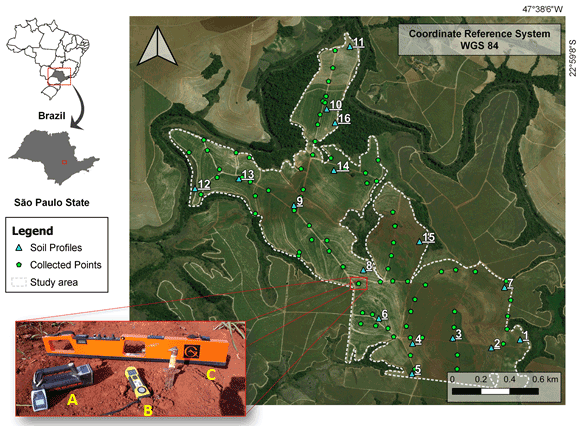
Figure 1 Study area, collection points, and geophysical sensors. A: gamma-ray spectrometer (Radiation Solution, RS 230);
B: susceptibilimeter (KT-10 Terraplus); C: Geonics Ground Conductivity Meter (EM 38).

The heterogeneity of the landform and the parent materials drove the formation of several soil types (Fig. 2b). Previous soil surveys and mapping have been performed in the study area by expert pedologists (Bazaglia Filho et al., 2013; Nanni and Demattê, 2006), in which the main soil classes mapped were as follows: Cambisols, Phaeozems, Nitisols, Acrisols, and Lixisols (IUSS Working Group WRB, 2014). Besides the soil profiles, 75 subsamples from 75 points (0–20 cm layer) were collected with an auger for physicochemical analyses, according to Fig. 1.

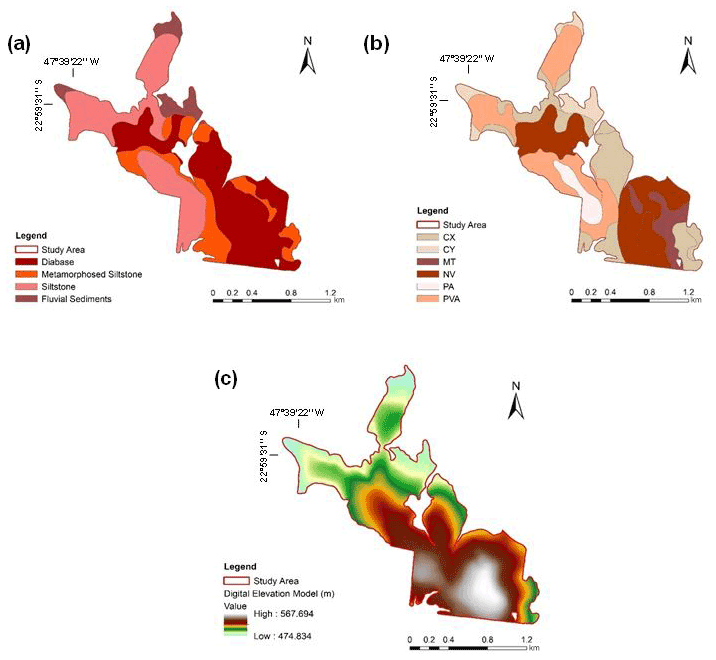
Figure 2 (a) Geological compartments of the landscape. (b) Soil classes – CX: Haplic Cambisols, CY: Fluvic Cambisols, MT: Luvic Phaozem, NV: Rhodic Nitisol: PA: Xanthic Acrisol, PVA: Rhodic Lixisol. The geological and soil class maps were adapted from Bazaglia Filho et al. (2012). (c) Digital elevation model.

According to the Köppen classification the region's climate is subtropical, mesothermal (Cwa), with an average temperature from 18 ^∘C (July–winter) to 22 ^∘C (February–summer), and a mean annual precipitation between 1100 and 1700 mm (Alvares et al., 2013).

2.2 Laboratory physicochemical analysis

For soil physical analyses, the soil samples were first air-dried, ground, and sieved through a 2 mm mesh, followed by granulometric analysis. After that, clay, silt, and sand contents were determined by the densimeter method (Camargo et al., 1986). Using the granulometry data, the textural groups were determined following the EMBRAPA (2011) methodology.

The exchangeable cations aluminum, calcium, and magnesium (Al³⁺, Ca²⁺, and Mg²⁺) were determined using KCl solution (1 mol L⁻¹) and quantified by titration (Teixeira et al., 2017). A Mehlich-1 solution was used to extract K⁺, which was quantified by flame photometry. Potential acidity (${\mathrm{H}}^{+}+{\mathrm{Al}}^{\mathrm{3}}$) was determined using a calcium acetate solution (0.5 mol L⁻¹) at pH 7.0; for the pH in water determination, the soil-to-solution ratio of 1:2.5 was used (Teixeira et al., 2017). More details about the analysis methods can be found elsewhere (Teixeira et al., 2017). Soil organic carbon was determined using the Walkley–Black method via oxidation with potassium (Teixeira et al., 2017; Pansu and Gautheyrou, 2006). The total iron content was determined using selective dissolution in sulfuric acid (Teixeira et al., 2017; Lim and Jackson, 1983). The resulting extract was used to determine the contents of silicon dioxide (SiO₂) and titanium dioxide (TiO₂), using the EMBRAPA methodology (2017). All other chemical parameters, such as base sum (BS) cation exchange capacity (CEC), base saturation (V %), and aluminum saturation (m %), were determined using the analytical data obtained previously, following the methodology described elsewhere (Teixeira et al., 2017).

2.2.1 Radionuclides and gamma-ray spectrometry data

The total radionuclide ⁴⁰K amount was measured by the absorption energy (1.46 MeV). Thorium (²³²Th) and uranium (²³⁸U) were quantified by absorption energy (approximately 2.62 and 1.76 MeV, respectively). This quantification was indirectly performed through thallium (²⁰⁸Tl) and bismuth (²¹⁴Bi), derived by radioactive decay, respectively, for ²³²Th and ²³⁸U, which are expressed as eTh and eU (equivalent thorium and uranium, respectively).

For soil gamma spectrometric characterization, we used the near-gamma-ray spectrometer (GM) model Radiation Solution RS 230 (Radiation Solution Inc., Ontario, Canada) (Fig. 1a). The sensor can quantify the eTh and eU concentrations in parts per million (ppm), whereas ⁴⁰K is quantified in percentage due to its major content in the pedosphere. Conventionally, radionuclides are expressed in mg kg⁻¹ for eU and eTh, whereas for ⁴⁰K, percentage is used. The GM detects the gamma-ray radiation emission down to a depth of 30–60 cm, which varies mainly with soil bulk density and moisture content (Wilford et al., 1997; Taylor et al., 2002; Beamish, 2015).

First, the GM was automatically calibrated by switching on and leaving the sensor on the ground surface for 5 min until readings of eU, eTh, and ⁴⁰K contents stabilized (Radiation Solutions, 2009). The measurements of radionuclides were taken in the “assay-mode” of the highest precision for quantification, in which the GM was kept at the soil surface for 2 min in each sampling point (79 total collection points) (Fig. 1). The geographic position was taken by a GPS coupled to the GM (GPS, Radiation Solution Inc., Ontario, Canada; precision of 1 m). The data collected from all points were concatenated with their respective information from the soil physicochemical analyses for later geoprocessing. The same methodology has been applied by Mello et al. (2021) for gamma-ray spectrometric data acquisition.

2.2.2 Magnetic susceptibility (κ)

For soil magnetic susceptibility (κ) characterization, surface readings were recorded at all 79 points, using a geophysical susceptibility meter sensor (KT10, Terraplus) (Fig. 1b). This sensor can measure κ to a depth of 2 cm below the soil surface, with a precision of 10⁻⁶ in SI units, expressed in m³ kg⁻¹. To perform the readings, the sensor was first calibrated by determining the frequency of the outdoor oscillator. Subsequently, we followed the sequence required to obtain the measurements performed in three steps: (1) determining the frequency and amplitude of the oscillator in free air; (2) measuring the frequency and amplitude of the oscillator with the coil placed directly on the soil surface (sample) outcrop; and (3) repeating step 1 and displaying the results. For more information about these procedures, see Sales, Support and Cusomisation (2021). We performed the readings in scanner mode, which uses the best geometric correlation to direct κ readings, providing fast and accurate quantification. We performed three readings in triangulation around each collection point and used the mean value of κ in all our analyses. This procedure was adopted to reduce noise. The same methodology for κ readings has been performed by Mello et al. (2020).

2.2.3 Apparent electrical conductivity (ECa)

The ECa measurements were performed using the conductivity meter Geonics EM38 (Geonics Ltd., Mississauga, Ontario, Canada) (McNeill, 1986) (Fig. 1c). The EM38 provides measurements of the quad-phase (conductivity) without any requirement for soil-to-instrument contact (Geonics, 2002); the unit is m mS⁻¹.

First, the EM38 was calibrated following the instructions of Heil and Schmidhalter (2019), Sect. 3.1.1. The values of ECa are a function of calibration, coil orientation, and coil separation (Heil and Schmidhalter, 2019). More details about the EM38 operation are provided in Hendrickx and Kachanoski (2002). After calibration, the ECa readings were performed at all 75 collection points (Fig. 1), using the EM38 at vertical dipole orientation, which provided data from an effective soil depth at 1.5 m. Data were collected in the field during the dry season, on bare soil, and at the same intervals to reduce the impacts of environmental variables. Also, all metal objects were kept away from the EM 38 to avoid reading interferences.

We developed our research and analysis by using three geophysical sensors (near-gamma-ray spectrometer RS 230, near-magnetic susceptibility sensor KT10, and conductivimeter Geonics EM38) due to the following reasons: these sensors are available in our institution and for our research partners, they are easy to operate, and the obtained data are highly accurate. In addition, the EM38 (conductivimeter) and RS 230 (gamma-ray spectrometer) provide information for the depth at which most of the pedogenetic processes occur. In addition, information obtained with EM38 and RS 230 can be associated with KT10 (susceptibilimeter) on the soil surface to provide additional information about some soil attributes related to soil subsurface horizons, which is also related to the other geophysical variables used (gamma-ray and apparent electrical conductivity).

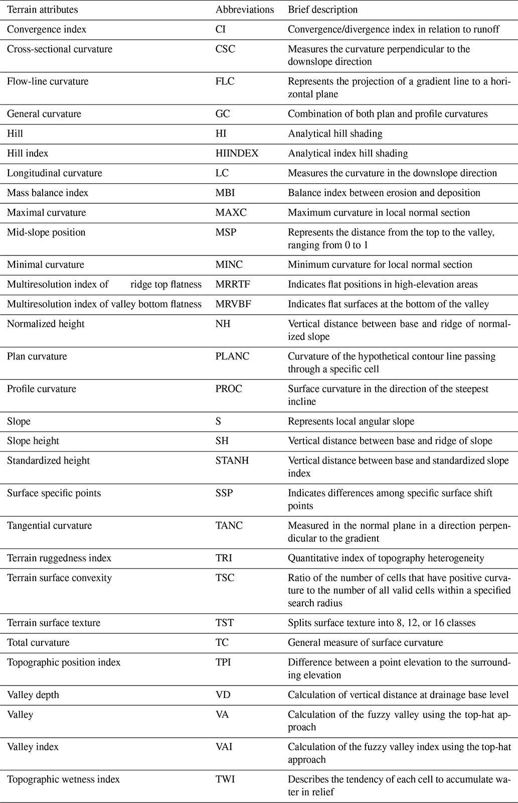
Table 1 Terrain variables generated from the digital elevation model.

2.2.4 Modeling processing

The modeling process is demonstrated in the flowchart (Fig. 3) and can be divided into two parts: the selection of covariates and the training/testing of the data. In the selection phase, the algorithm tries to produce the ideal set of covariates, following the principle of parsimony. This is performed by removing highly correlated variables, evaluating the importance of covariables, and removing variables that have a minor importance in training the model in the prediction process of each algorithm. Darst et al. (2018) considered the joint application of the methods for the selection of covariates by correlation and importance (RFE) since the use of RFE only reduces the effect of highly correlated covariates but does not eliminate it.

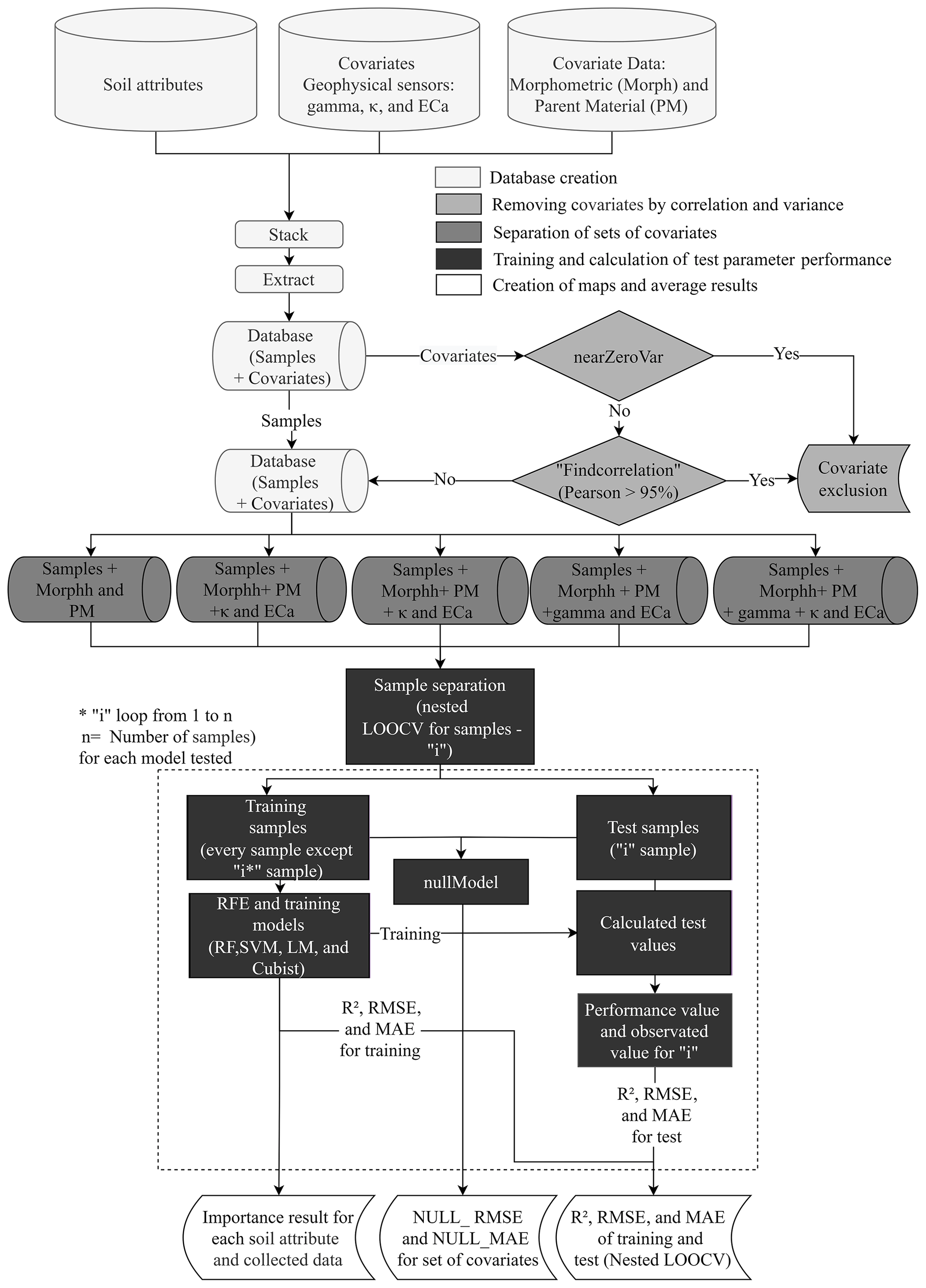
Figure 3 Methodological flowchart showing the sequence of methodologies applied for soil and geophysical attribute prediction. The most accurate model among Cubist, random forest (RF), support vector machines (SVMs), and linear models (LMs) was selected to model and map the geophysical and soil attributes.

The correlation selection process was used to calculate the correlation of the set of covariates and covariables, which were evaluated with a correlation greater than the limit (Pearson test >95 %). The pairs that showed higher values were evaluated due to their correlation with the complete set of covariates, eliminating that with the highest value of the sum of the absolute correlation with the other covariables that started in this process. For this phase, we applied the “cor” and “find correlation” functions of the “stats” (Hothorn, 2021) and “caret” (Kuhn et al., 2020) packages, in the R software, respectively (Kuhn and Johnson, 2013). In this phase, the covariables curv_cross_secational and curv_longitudinal were eliminated for all tested sensor sets. The set of covariables that passed this phase joined the samples followed by the separation of samples from training and testing.

The separation of training and testing was performed using the “nested” leave-one-out (nested-LOOCV) method (Clevers et al., 2007; Honeyborne et al., 2016; Rytky et al., 2020). It is important to highlight that the number of soil samples and readings with geophysical sensors was small (75) due to several difficulties encountered in the field during data collection (high sugar cane size, sloping terrain, dense forest, etc.). In this sense, the nested LOOCV method is indicated for small sample sets (values near 100 samples) to which other validation/testing methods (such as holdout validation) would not be viable due to the small sample set in the testing and/or training group (Ferreira et al., 2021). This is one of the main innovations of this research.

The nested LOOCV method is a double-loop process. In the first loop, the model is trained with a data set of size n−1, and the test is done in the second loop with the missing sample to validate the training performance (Jung et al., 2020; Neogi and Dauwels, 2022). The final results of the performance of the machine learning algorithm will be the mean performance indicators for all points (training/testing). This is a robust method to evaluate the performance of the algorithm and to detect possible samples with problems in the collections or outliers. The training set generated in each loop went through the process of selecting covariates for importance and subsequent training.

The selection of covariates by importance is performed using the back forward method, applying the recursive feature elimination (RFE) function contained in the caret package (Kuhn and Johnson, 2013). The RFE is unique for each algorithm, with the result being the set of selected covariates used in the prediction of the final model in the same algorithm. The RFE is a selection method that eliminates the variables that least contribute to the model, based on a measure of importance for each algorithm (Kuhn and Johnson, 2013). The algorithm will be applied to complete sets of data (variable by the set of tested sensors) and 18 more subsets with 5, 6, 7, … 19, 20, and 30 covariables. Reaching a set of fewer variables (more parsimonious) results in a better prediction performance. The optimization of the ideal covariate subset was based on LOOCV, a repetition, and four values of each of the internal hype parameters of each tested algorithm (“tune length”). The hyperparameters of each algorithm are described in the caret package manual in chapter 6, “Models described”, available at https://topepo.github.io/caret/train-models-by-tag.html (last access: 1 February 2022). The metric for choosing the best subset for each model was R². For this work, five algorithms were tested: random forest (RF), Cubist (C), support vector machines (SVMs), and generalized linear models (LMs). The choice was made with the use of families of different algorithms in mind, using linear and non-linear algorithms. The algorithms used are commonly applied in soil attribute mapping studies. At the end of the selection phase by importance, the most optimized set of covariates for training was generated for each algorithm.

Training was performed with the variables selected in the previous step and each tested algorithm by using LOOCV and 10 repetitions. Four values of each of the internal hype parameters of each tested algorithm were also tested (tune length). At the end of the training phase, a sample prediction was made that was not used in the training, and the result was saved for the performance study. The performance of the prediction of the algorithms and the set of sensors was determined with a set of samples from the outer loop of the nested-LOOCV method. Three evaluation parameters were used: R squared, R² (Eq. 1); root mean squared error, RMSE (Eq. 2); mean absolute error, MAE (Eq. 3).

$$\begin{array}{}\text{(1)}& R^{\mathrm{2}}={\displaystyle \frac{{\left[\sum \left(Q{}_{\mathrm{pred}}-\stackrel{\mathrm{‾}}{Q_{\mathrm{pred}}}\right)\times \left(Q_{\mathrm{obs}}-\stackrel{\mathrm{‾}}{Q_{\mathrm{obs}}}\right)\right]}^{\mathrm{2}}}{\left[\sum {\left(Q_{\mathrm{pred}}-\stackrel{\mathrm{‾}}{Q_{\mathrm{pred}}}\right)}^{\mathrm{2}}\right]\times \left[\sum {\left(Q_{\mathrm{obs}}-\stackrel{\mathrm{‾}}{Q_{\mathrm{obs}}}\right)}^{\mathrm{2}}\right]}},\end{array}$$

$$\begin{array}{}\text{(2)}& {\displaystyle }\mathrm{RMSE}=\sqrt{{\displaystyle \frac{\mathrm{1}}{n}}\times \sum {\left(Q_{\mathrm{obs}}-Q_{\mathrm{pred}}\right)}^{\mathrm{2}}},\text{(3)}& {\displaystyle }\mathrm{MAE}={\displaystyle \frac{\mathrm{1}}{n}}\times \sum \left|Q_{\mathrm{pred}}-Q_{\mathrm{obs}}\right|,\end{array}$$

where Q_pred denotes predicted samples, Q_obs denotes observed samples, and n denotes the number of samples.

For comparison purposes, null model values (NULL_RMSE and NULL_MAE) were also calculated. The null model considers using the average value quantified by the collected samples (Eqs. 4 and 5). The null model (NULL_RMSE and NULL_MAE) emulates other model-building functions but returns the simplest model possible given a training set: a single mean for numeric outcomes. The percentage of the training set samples with the most prevalent class is returned when class probabilities are requested. The null model can be considered the simplest model that can be adjusted and that serves as a reference. Models that present similar or worse performances compared to the null model should be discarded. The best models had lower RMSE and MAE results than those found for NULL_MAE and NULL_RMSE. This shows that the final model is better than using the mean values, which also demonstrates a better quality in creating the models.

Given the above, the null model considers using the mean value quantified by the collected samples (Eqs. 4 and 5). This methodology is widely used, as well as spatialization processes in kriging when the variable in which spatialization is desired has spatial dependence (pure nugget effect). The equations are as follows:

$$\begin{array}{}\text{(4)}& {\displaystyle }\mathrm{NULL}\mathrm{\_}\mathrm{RMSE}={\left[{\displaystyle \frac{\mathrm{1}}{N}}{\sum }_{i=\mathrm{1}}^N{\left({\stackrel{\mathrm{‾}}{Q_{\mathrm{train}}}}_{{}_i}-Q_{{\mathrm{obs}}_i}\right)}^{\mathrm{2}}\right]}^{\frac{\mathrm{1}}{\mathrm{2}}},\text{(5)}& {\displaystyle }\mathrm{NULL}\mathrm{\_}\mathrm{MAE}={\displaystyle \frac{\mathrm{1}}{n}}\times \sum \left|{\stackrel{\mathrm{‾}}{Q_{\mathrm{train}}}}_{{}_i}-Q_{{\mathrm{obs}}_i}\right|,\end{array}$$

where Q_train denotes the mean of the training samples, Q_obsi denotes the validation sample, N denotes the number of samples (loop).

Here NULL_RMSE and NULL_MAE values lower than those observed in the prediction of the algorithm in the validation phase show that the use of means of the samples of the desired propriety agrees with the model created by the algorithms of the machine learning. The NULL_RMSE and NULL_MAE were calculated using the “null mode” function of the caret package (Kuhn et al., 2020).

The final result of the performance of the algorithms of each attribute was obtained using the 75 loops, with the training results being the average of the performance and the results of the test samples calculated from the 75 external loops results using Eqs. (1)–(3). The importance of the algorithms was calculated by the caret package (Kuhn and Johnson, 2013); each model presents its creation methodology. The final importance for each algorithm and attribute was determined from the importance created in the loop, being the average of the importance of the 75 repetitions.

3 Results

3.1 Geophysical sensor combinations, model performance, uncertainty, and covariate importance

The worst performance in modeling soil attributes occurred excluding the use of geophysical sensors (non-use of the geophysical sensor), where only parent material and terrain attributes were used (Table 2). In this case, the algorithms selected particular groups of terrain attributes for the modeling of each soil attribute (Table 1).

Table 2 Model performance for non-use geophysical sensors, for all soil attributes, based on R², RMSE, MAE, and NULL_RMSE.

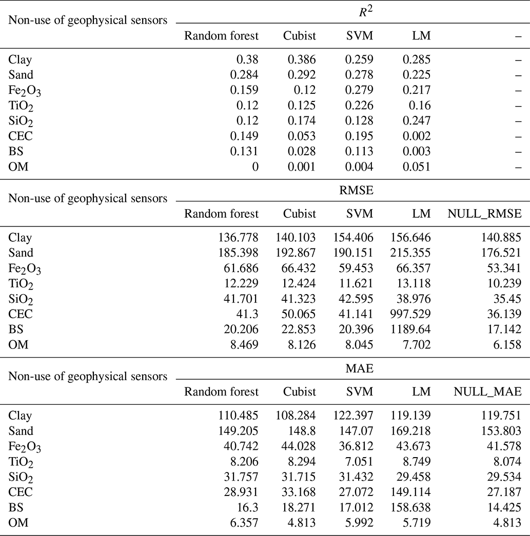
CEC: cation exchange capacity; SVM: support vector machine; LM: linear model; BS: base saturation; OM: organic matter. Clay and sand content in g kg⁻¹; Fe₂O₃, TiO₂, and SiO₂ in g kg⁻¹; CEC in mmol_c dm⁻³, OM in g dm⁻³; BS in mmol_c dm⁻³.

The Cubist algorithm (non-use of the geophysical sensor) showed the best performance in predicting soil texture, clay (R² of 0.386), and sand (R² of 0.292) contents, with the highest R² and the lowest RMSE and MAE values, concomitantly (Table 2). The importance of covariates to sand content prediction showed that minimal curvature was the most important variable, contributing 100 % to the decrease mean accuracy. On the other hand, for clay content, the most important variable was parent material. In addition, for clay and sand, the tangential curvature and DEM showed an importance higher than 50 % (Fig. 4).

When the geophysical sensor was not used, the SVM algorithm presented a moderate performance for Fe₂O₃ (R² 0.279) and TiO₂ (R² 0.226), whereas for SiO₂, the LM presented the best result, also with a moderate performance (R² 0.247) (Table 2). The selected models simultaneously presented the highest R² and lowest RMSE and MAE values. The most important covariates for Fe₂O₃ and TiO₂ prediction by the SVM model were parent material (100 %) and DEM (more than 50 %). For SiO₂ prediction by the LM, the most important covariates were DEM (100 %) and standardized height (90 %), whereas parent material contributed 40 % (Fig. 4).

For cation exchange capacity (CEC), the model with the best performance after 75 runs was SVM (R² of 0.223) (Table 2) when the geophysical sensor was not used. The most important covariates for CEC prediction to mean accuracy were DEM (100 %), topographic wetness index (80 %), and parent material (75 %) (Fig. 4).

Figure 4 Variable importance for non-use of geophysical sensors (only variables that contributed more than 50 % are presented here). For further details, see Supplement.

All models showed a low performance in the prediction of base saturation (BS) and organic matter (OM), with R² values between 0.001 and 0.1 (Tables 2–6).

The different combinations of geophysical sensors that contributed to the moderate modeling performance for soil attributes were as follows: susceptibilimeter + conductivimeter (S + C), gamma-ray spectrometer + conductivimeter (G + C), and combined use of the three geophysical sensors ($G+S+C$) (Tables 3, 4, and 6, respectively). The R² values presented some variations between the R² of the best combination of geophysical sensors and the lowest R² values when the geophysical sensors were not used in the predictive models (Tables 3, 4, and 6). Among all the values of R² evaluated for this session, we considered all the highest values; among the highest values, we considered the lowest values as the worst results.

Table 3 Model performance for the combined use of susceptibilimeter and the conductivimeter, for all soil attributes, based on R², RMSE, MAE, and NULL_RMSE.

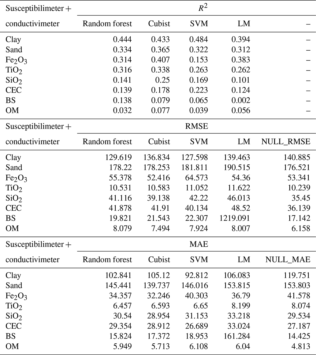
CEC: cation exchange capacity; SVM: support vector machine; LM: linear model; BS: base saturation; OM: organic matter. Clay and sand content in g kg⁻¹; Fe₂O₃, TiO₂, and SiO₂ in g kg⁻¹; CEC in mmol_c dm⁻³, OM in g dm⁻³; BS in mmol_c dm⁻³.

Table 4 Model performance for the combined use of gamma-ray spectrometer and the conductivimeter, for all soil attributes based on R², RMSE, MAE, and NULL_RMSE.

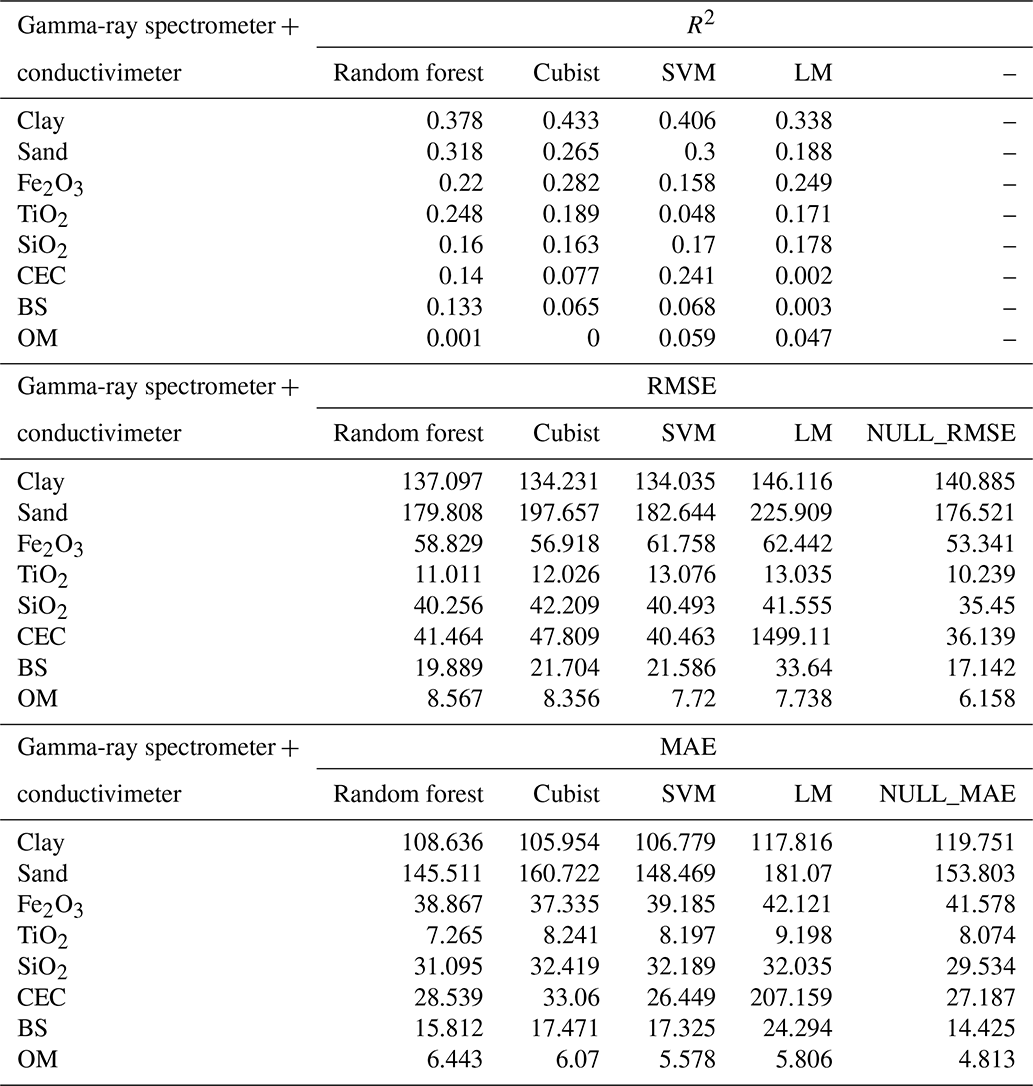
CEC: cation exchange capacity; SVM: support vector machine; LM: linear model; BS: base saturation; OM: organic matter. Clay and sand content in g kg⁻¹; Fe₂O₃, TiO₂, and SiO₂ in g kg⁻¹; CEC in mmol_c dm⁻³, OM in g dm⁻³; BS in mmol_c dm⁻³.

For clay, the model with the best performance was the SVM algorithm (R² 0.484) using S + C (Table 3), whereas that with the worst performance was the Cubist algorithm (R² 0.38) using $G+S+C$ (Table 6). For sand, the best model performance was obtained with the Cubist algorithm (R² 0.365) using S + C (Table 3) and the worst also by Cubist (R² 0.387) using $G+S+C$. The most important covariates for clay prediction by the SVM model in the S + C sensor combination were magnetic susceptibility (κ) (100 %) and parent material (90 %) (Fig. 5). For clay prediction by the Cubist model in the $G+S+C$ sensor combination, the most important covariate was parent material (100 %) (Fig. 6). With respect to sand prediction, the most important covariates by the Cubist model in S + C were minimal curvature (100 %) and magnetic susceptibility (κ) (80 %) (Fig. 5). On the other hand, for $G+S+C$, the covariates that most contributed to sand prediction were DEM (100 %), general curvature (80 %), and minimal curvature (75 %) (Fig. 6).

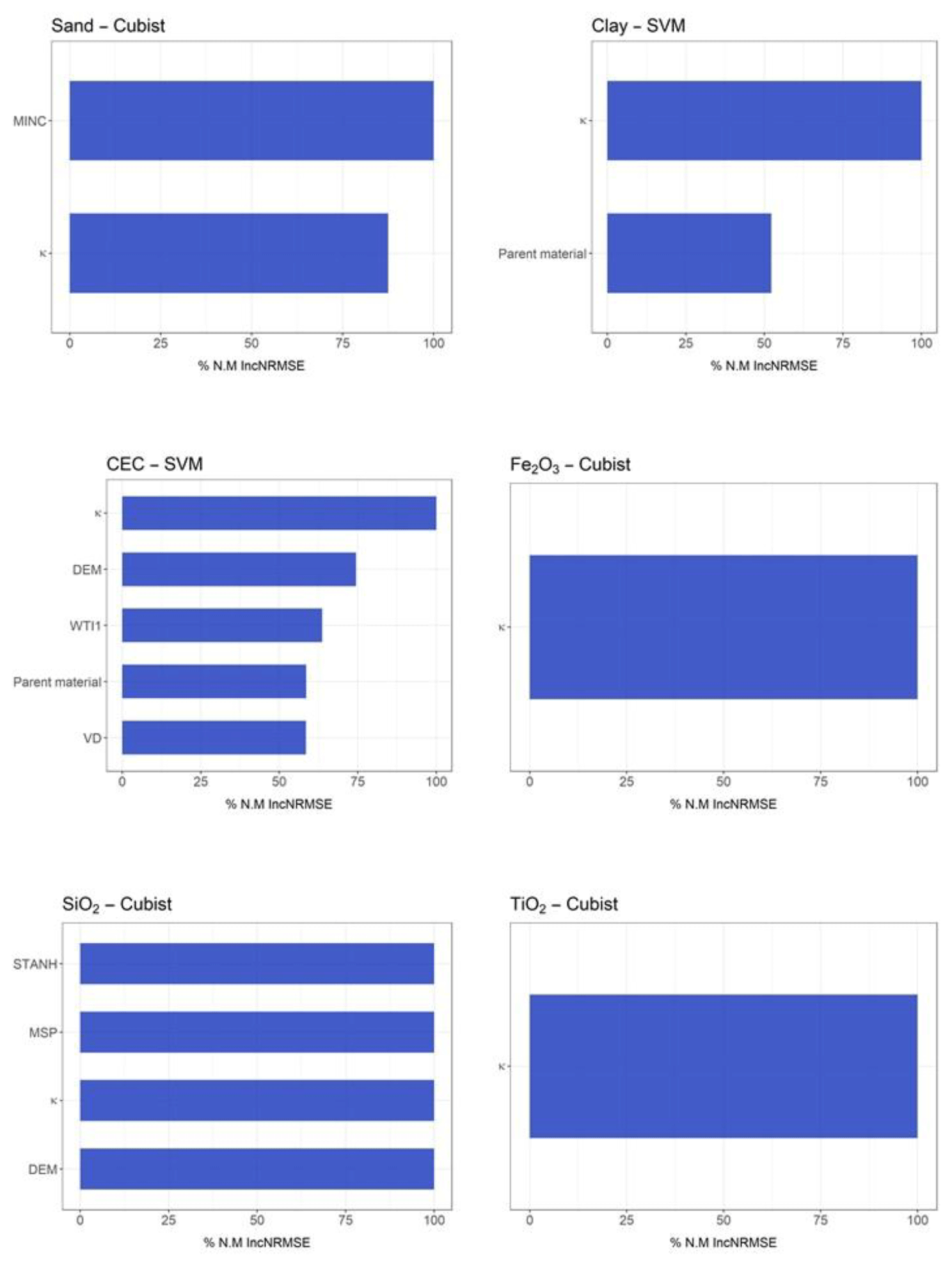
Figure 5 Variable importance for susceptibilimeter + conductivimeter sensors (only variables that contributed more than 50 % are presented here; for further details see Supplement).

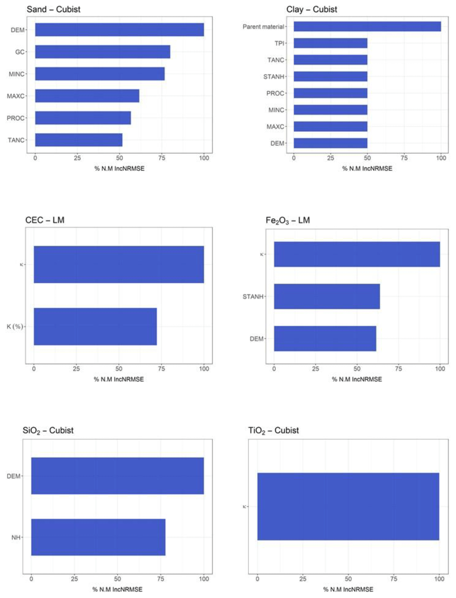
Figure 6 Variable importance for combined use of the three geophysical sensors (only variables that contributed more than 50 % are presented here; for further details see Supplement).

For the elemental composition, the models employed greatly variable performance. For Fe₂O₃ the best model performance was reached by the LM algorithm (R² 0.441) using $G+S+C$ (Table 6), while the worst performance was by the Cubist (R² 0.282) using G + C (Table 4). With respect to TiO₂, the best model performance was by the Cubist algorithm (R² 0.358) using $G+S+C$ (Table 6) and the worst was RF (R² 0.248) using G + C (Table 4). For SiO₂, the best model performance was the Cubist algorithm (R² 0.250) using S + C (Table 3) and the worst was the LM (R² 0.178) using G + C (Table 4). The importance of covariates in predicting Fe₂O₃ by LM in $G+S+C$ demonstrated that magnetic susceptibility (κ), standardized height, and DEM were the most important variables, contributing 100 %, 65 %, and 55 %, respectively (Fig. 6). For Fe₂O₃ predicted by the Cubist algorithm using G + C, the most important covariates were standardized height, parent material, ECa, and DEM (100 %) (Fig. 7). For TiO₂ prediction by the Cubist algorithm using $G+S+C$ the most important covariate was magnetic susceptibility (κ) (100 %) (Fig. 6), while for the RF algorithm using G + C, they were parent material (100 %) and ECa (75 %) (Fig. 7). In relation to SiO₂ prediction by the Cubist using S + C, the most important covariates were standardized height, mid-slope position magnetic susceptibility (κ), and DEM (100 %) (Fig. 5), while those for SiO₂ predicted by the LM algorithm using G + C were DEM and standardized height (100 % and 65 %, respectively) to mean accuracy (Fig. 7).

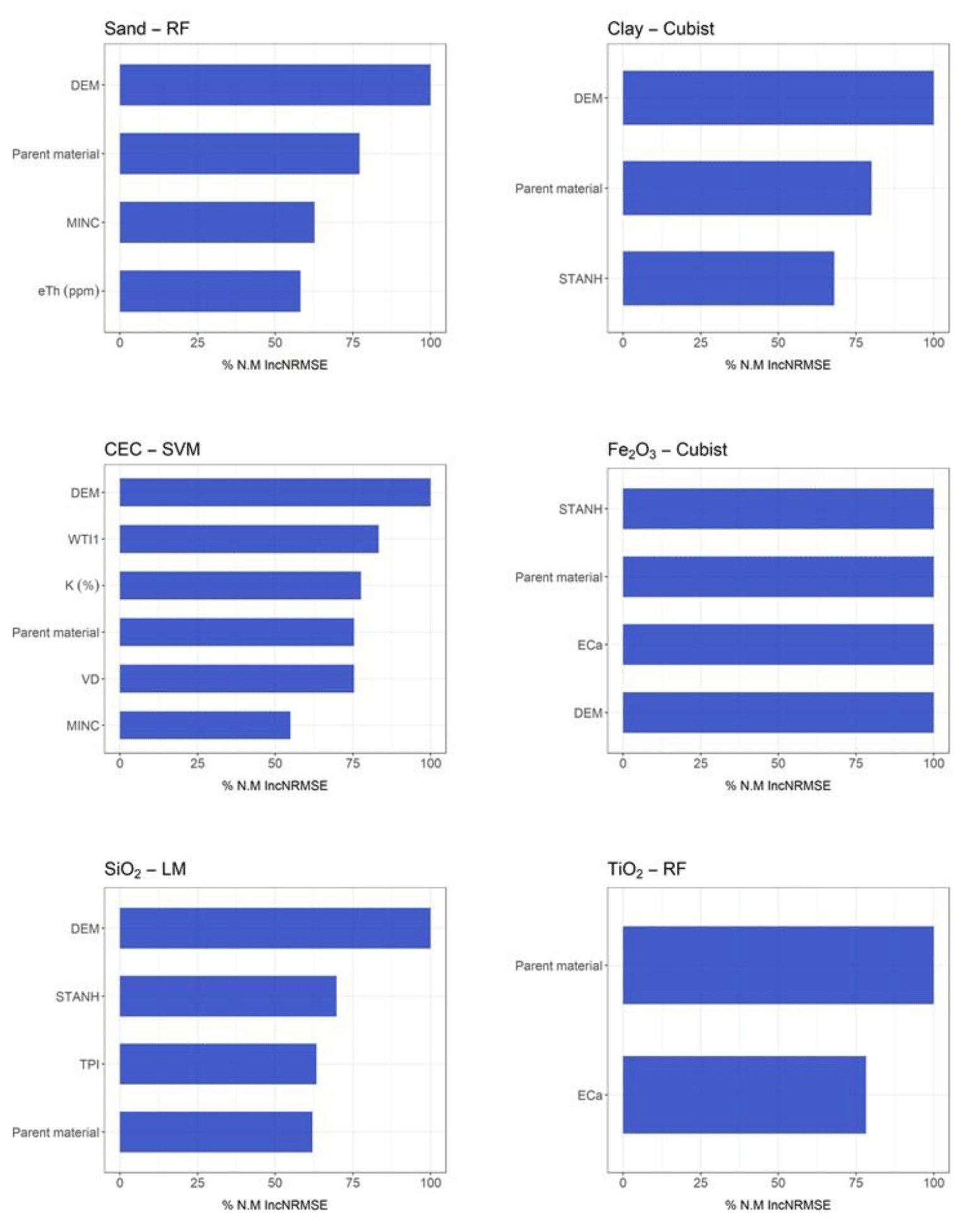
Figure 7 Variable importance for gamma-ray spectrometer + conductivimeter sensors (only variables that contributed more than 50 % are presented here; for further details see Supplement).

In relation to CEC, the LM algorithm was the best model (R² 0.317) using $G+S+C$ (Table 6) and the worst was the SVM algorithm (R² 0.223) using S + C (Table 3). The most important covariate for prediction of CEC by the LM algorithm using $G+S+C$ and using S + C was magnetic susceptibility (κ) (100 %) (Figs. 5 and 6).

Overall, the best combination of geophysical sensors, which allowed the best model performance for different algorithms in the prediction of soil attributes, was gamma-ray spectrometer + susceptibilimeter (G + S) (Table 5).

Table 5 Model performance for combined use of gamma-ray spectrometer and susceptibilimeter, for all soil attributes, based on R², RMSE, MAE, and NULL_RMSE.

CEC: cation exchange capacity; SVM: support vector machine; LM: linear model; BS: base saturation; OM: organic matter. Clay and sand content in g kg⁻¹; Fe₂O₃, TiO₂, and SiO₂ in g kg⁻¹; CEC in mmol_c dm⁻³, OM in g dm⁻³; BS in mmol_c dm⁻³.

Table 6 Model performance for all combined use of geophysical sensors, for all soil attributes, based on R², RMSE, MAE, and NULL_RMSE.

CEC: cation exchange capacity; SVM: support vector machine; LM: linear model; BS: base saturation; OM: organic matter. Clay and sand content in g kg⁻¹; Fe₂O₃, TiO₂, and SiO₂ in g kg⁻¹; CEC in mmol_c dm⁻³, OM in g dm⁻³; BS in mmol_c dm⁻³.

For soil texture, the SVM and RF algorithms showed the best performance for clay (R² 0.494) and sand (R² 0.422), respectively, using G + S, with the highest R² and lowest RMSE and MAE values (Table 5). The importance of covariates in predicting soil texture by the SVM (for clay) and the RF (for sand) demonstrated that magnetic susceptibility (κ) was the most important covariate (100 %). In addition, parent material contributed 60 % for clay prediction and DEM 60 % for sand prediction (Fig. 8).

The LM algorithm presented the best performance for Fe₂O₃ (R² 0.470) and TiO₂ (R² 0.328), using G + S, whereas for SiO₂, the Cubist algorithm was the most suitable (R² 0.207), also using G + S (Table 5). The most important covariates for Fe₂O₃ and TiO₂ prediction via LM using G + S were magnetic susceptibility (κ) and standardized height (100 % and 60%, respectively, for both) (Fig. 8). For SiO₂ prediction via the Cubist algorithm using G + S, the most important covariates were mid-slope position and magnetic susceptibility (κ) (100 % for both) (Fig. 8).

For CEC, the best model performance was obtained using the LM algorithm (R² 0.303) using G + S (Table 5). In this case, the covariates that most contributed to model prediction were magnetic susceptibility (κ) (100 %) and DEM (60 %) (Fig. 8).

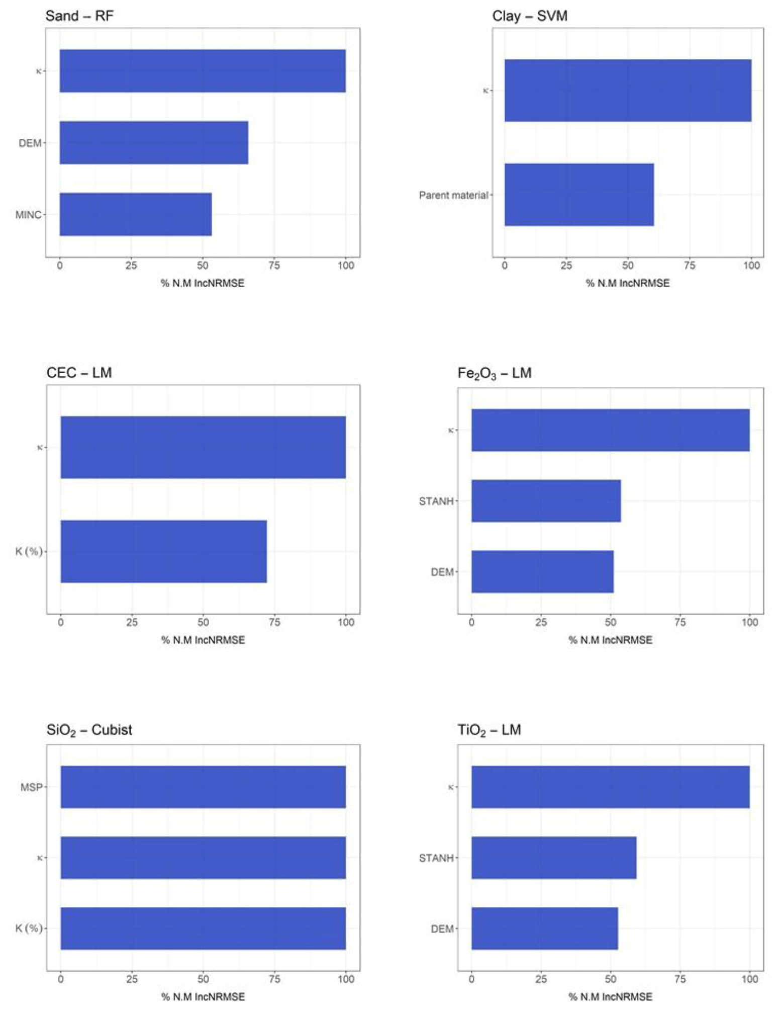
Figure 8 Variable importance for gamma-ray spectrometer + susceptibilimeter sensors (only variables that contributed more than 50 % are presented here; for further details see Supplement).

4 Discussion

4.1 Geophysical sensor combinations, models performance, and uncertainty

The methodological approach optimized the prediction of soil variables by applying different geophysical sensor combinations, parent material, and terrain attributes for selecting covariates and models, as well as for assessing prediction uncertainty.

In general, without the use of geophysical sensors, the poorest results were obtained in terms of R², RMSE, and MAE for all prediction algorithms used for modeling soil attributes (Table 2). These results are consistent with Frihy et al. (1995), who also compared the combined use and the non-use of sensors regarding model geochemical attributes of soil by the Cubist algorithm and obtained the worst results without using the sensors. Most likely, this is a result of the highly complex interaction between soil forming factors and processes determining soil attributes (Jenny, 1994).

The moderate performance of the models can be attributed to the different combinations of the geophysical sensors pairwise, and the different data presented by the sensors contributed in different ways to the modeling process. In this regard, O'Rourke et al. (2016) also demonstrated a moderate performance of the models (R² ranging from 0.21 to 0.94) when using data from the Vis-NIR, with R² ranging from 0.61 to 0.94 when using the pXRF sensor to model soil attributes. This might be related to the different sensors and their relation with soil attributes. The Vis-NIR spectroscopy acts on targets with low energy levels, showing the ability to identify soil mineral species, strongly linked to soil attributes (Coblinski et al., 2021). In addition, pXRF spectroscopy allows the identification of total elementary contents by acting with high levels of ionizing energy, which is not identified by Vis-NIR and is strongly correlated with minerals and soil attributes (Silvero et al., 2020). Therefore, the addition of pXRF with Vis-NIR data for obtaining information about soil constituents is highly efficient for modeling soil attributes.

The best combination of geophysical sensors was gamma-ray spectrometer + susceptibilimeter (G + S), with the highest values of R² and the lowest values of RMSE and MAE (Table 5). Most likely, the gamma-ray spectrometer and the susceptibilimeter are more closely associated with pedogenesis (argilluviation, ferralitization, and others), pedogeomorphology, and soil attributes, as recently demonstrated by Mello et al. (2020, 2021), who modeled soil attributes such as texture, Fe₂O₃, TiO₂, SiO₂, and CEC in relation to thorium, uranium, and potassium (⁴⁰K) levels as well as magnetic susceptibility.

In general, the Cubist algorithm was the best model for clay and sand content prediction (Table 7). Similar results have been found by Greve and Malone (2013); Ballabio et al. (2016); Nawar et al. (2016); and Silva et al. (2019), who used the Cubist and Earth algorithm to predict soil texture using different data sources (3D imagery, Land Use and Coverage Area frame Survey, and reflectance spectroscopy). In all these models, the R² was not greater than 0.5, which can be explained by the small variation or limited distribution of the data set, causing poor modeling prediction. Zhang and Hartemink (2020) state that textural classes with fewer samples presented a more unstable prediction performance than those with more samples, which agrees with our results.

Table 7 Number of times that each model achieved the best performance for each soil attribute.

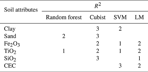
CEC: cation exchange capacity; SVM: support vector machine; LM: linear model; BS: base saturation; OM: organic matter. Clay and sand content in g kg⁻¹; Fe₂O₃, TiO₂, and SiO₂ in g kg⁻¹; CEC in mmol_c dm⁻³, OM in g dm⁻³; BS in mmol_c dm⁻³.

The better performance for elemental composition (Fe₂O₃, TiO₂, and SiO₂) was obtained using the Cubist algorithm (Table 7), with an R² of 0.2–0.47. This is contrasting with the results obtained by Henrique et al. (2018), who showed that the best model for predicting soil mineralogy Fe₂O₃ and TiO₂ (R² 0.89 and 0.96, respectively) and RF only for Fe₂O₃ (R² 0.95) by pXRF was the simple linear regression. In our study, the R² variation for the G + S combination was probably related to the low correlation with the parent material and, consequently, with soil mineralogy or to the limited number of samples and the high soil variability (Fiorio, 2013). However, it is important to highlight that in situ, various intrinsic environmental influences can interfere with modeling processes. For example, the relatively low R² values (approximately between 0.2 and 0.5) can be attributed to the difficulty in modeling soils and their attributes. This is related to the high complexity of soils, such as the high spatial variability in surface and depth; the occurrence of geomorphic processes, weathering, and pedogenesis; and the different soil formation factors. For soil mineralogical attributes predicted by machine learning algorithms, the results can be classified as satisfactory from 0.2 to 0.5, as for the preliminary evaluation, since these values represent more informative results (Beckett, 1971; Dobos, 2003; Malone et al., 2009). According to Nanni and Demattê (2006), the R² may be explained by standardized laboratory conditions (such as temperature, humidity, substance concentrations, and other variables that interfere with the analysis results during their determination), with less environmental interference compared with direct field methods.

For CEC, the best model performance was obtained for SVM (R² 0.296) (Table 5). This result is corroborated by Liao et al. (2014), who compared the model performance of multiple stepwise regression, artificial neural network models, and SVM for CEC prediction and attributed their results to a nonlinear relationship between CEC and soil physicochemical properties. In addition, in our previous study (Jafarzadeh et al., 2016), we demonstrated that, despite the ability of SVM to predict CEC in acceptable limits, there is a poor performance in extrapolating the maximum and minimum values of CEC data. Despite this, uncertainties estimated for SVM predictions may not be associated with an incorrect classification, as pointed out by Cracknell and Reading (2013).

Even for the best combination of sensors (G + S) and the highest overall model performance, the R² values were not greater than 0.5 (Table 5). In models generated by field data, without sample preparation, R² values varying between 0.20 and 0.50 can be considered satisfactory and reliable (Dobos, 2003; Malone et al., 2009). In our study, the low R² values can be related to the limited number of collecting points or to the low field distribution, which does not represent the spatial variation of soil attributes; this is in agreement with Johnston et al. (1997) and Lesch et al. (1992), who evaluated soil salinity.

The best results for predictors of soil attributes through geophysical data have the lowest values when compared to the values of NULL_RMSE and NULL_MAE. This demonstrates that the use of machine learning models has less errors than the use of mean values for the entire area (Table 5), resulting in a better performance and accuracy.

The null model is a simple model (naive) that expresses the value of the mean of the Y (variable to be predicted or target variable). The RMSE and MAE values are calculated for the null model and further compared with MAE and RMSE values calculated by other models. If the RMSE and MAE values from other models present similar or worse performance than the null model, the model that compared it is not an informative model. In this case, it is better to choose a simple mean as a predictor rather than using a more complex model to explain a given phenomenon. The null model sets a minimum performance threshold to be reached by models (Kuhn et al., 2020); however, there are only few studies using NULL_RMSE and NULL_MAE as parameters for model evaluation and decision making.

4.1.1 Variables importance, model performance, and pedogeomorphology

In general, for all geophysical sensor combinations, the majority of terrain attributes used did significantly influence sand and clay content prediction (Figs. 4–6 and 8). However, in most cases, parent material and magnetic susceptibility strongly influenced clay content prediction, except for G + C (Fig. 7). Ließ et al. (2012) found that the best performance was obtained using the RF model, with elevation and overland flow distance strongly affecting the model performance. According to Bauer (2010), the greater sand$/$clay ratio upslope is explained by the selective transport of fine material downslope, whereas in the present study, the clay content increased because of the influence of parent material (diabase), as also demonstrated by Mello et al. (2020).

Magnetic susceptibility (κ), followed by DEM and parent material, were the key variables that contributed to sand and clay content prediction by RF and SVM, respectively, for G + S (Fig. 8). Siqueira et al. (2010) and Mello et al. (2020) found a positive correlation between soil magnetic susceptibility and clay content and a negative correlation between magnetic susceptibility and sand content. In fact, the mineralogical composition of the parent material strongly affects soil magnetic susceptibility (Ayoubi et al., 2018), mainly in tropical soils under the top of basalt spills (Da Costa et al., 1999), where our study was undertaken.

In general, for Fe₂O₃ and TiO₂, the most important variables were parent material, magnetic susceptibility, and DEM, which, in most cases, contributed 100 % (Figs. 4–8). In fact, the mineralogical composition of the parent material and the pedoenvironmental conditions strongly influence the amount of Fe $/$ Ti oxides in soils (Schwertmann and Taylor, 1989; Kämpf and Curi, 2000; Bigham et al., 2002) and accelerate redistribution by downslope erosion (Mello et al., 2020). Also, the mineralogical composition of the parent material (Mullins, 1977; Ayoubi et al., 2018) and the landform evolution (Blundell et al., 2009; Sarmast et al., 2017) control the magnetic susceptibility of soil. Since the sensors used record the surface response and topography effect, it is expected that the most important variables indicated by the models would be related to surface processes. For the best combination of sensors (G + S), magnetic susceptibility and standardized height were more important variables in the prediction of Fe₂O₃ (100 %) and TiO₂ (55 %) contents (Fig. 8), corroborating the expected surface processes and materials in the magnetic susceptibility of the soil (Shenggao, 2000; Damaceno et al., 2017) and the relief in the distribution of these materials (De Jong et al., 2000).

For SiO₂, the most important variable was DEM, which, in most cases, contributed 100 % (Figs. 4–7). The level of SiO₂ in soil is directly related to the nature of the parent material and the erosion processes at different topographic positions (Bockheim et al., 2014; Breemen and Buurman, 2003). This can explain the greater contribution of the DEM in the prediction models. For the best sensor combination (G + S), the variable that most contributed was mid-slope position, which also is related to topographic features.

For CEC, the variables DEM and magnetic susceptibility were the most important ones, contributing 100 % in most of the cases (Figs. 4–8). This can be explained by the high correlation between magnetic susceptibility, clay content, and CEC (Siqueira et al., 2010; de Souza Bahia et al., 2017; Mello et al., 2020). These variables vary with parent material and surface geomorphic processes, concentrating ferrimagnetic minerals (Frihy et al., 1995; Mello et al., 2020).

Considering that the gamma-ray spectrometer sensor is composed of three channels (eU, eTh, and ⁴⁰K), it can be called “three sensors”. Thus, considering the combination of sensors used, it is possible to create a modeling performance graph using the number of sensors used through learning curves (Fig. 9). Such a learning curve shows a measure of the predictive performance of a given domain as a function of some measurements of varying amounts of learning effort (Perlich, 2010). In our case, the varying amounts were the number of sensors: non-use of geophysical sensors (zero sensors), S + C (two sensors), G + S (four sensors), and $S+G+C$ (five sensors). In this analysis, the combination of G + C sensors will not be used because they present the same number of G + S sensors (four sensors). However, the combination G + C presented lower results than G + S.

For five soil properties (clay, sand, CEC, Fe₂O₃, and SiO₃), the best results did not occur with a greater number of sensors, showing that increasing the number of covariables can lead to a lower performance (Fig. 9). This fact is associated with the addition of a new sensor as a covariate, which may provide conflicting information for the set of the other sensors found, where the ECa may have presented conflicting values with the sensors generated by the gamma-ray spectrometry channels, which generates a loss of performance when sensors are combined. The application of the RFE importance selection method was able to amortize this, making it a reliable method to reduce this effect.

Figure 9 Learning curves calculated on the metric by which the parameters of the model were optimized and on the metric by which the model was evaluated and selected. The most common form of learning curves in the general field of machine learning shows predictive accuracy on the test examples as a function of the number of training examples (Perlich, 2010).

0-NU denotes non-use of geophysical sensors; 2-S + C denotes two channels corresponding to susceptibilimeter + conductivimeter; 3-G denotes three channels corresponding to eU, eTh and ⁴⁰K from gamma-ray spectrometer; 4-G + S denotes four channels corresponding to eU, eTh and ⁴⁰K from gamma-ray spectrometer + susceptibilimeter.

4.1.2 General evaluation

For this study, the independent RMQS data set was not large enough (75 sites). Therefore, validation using 74 sites provided erratic and inconsistent results, mainly when comparing different pedoenvironmental indicators, even considering that this data set, in theory, provides “unbiased” estimates of forecast performance (Loiseau et al., 2020). Similarly, Lagacherie et al. (2019) showed that the location and number of samples used for independent assessment can significantly impact the values of these indicators. This indicates that the greatest variations were observed for evaluation sets with less than 100 samples.

Modeling soil attributes using relief and geophysical data presented promising results for geoscience studies and soil scientists. The use of several algorithms from different “families”, as well as the training and validation method, also made the study more robust and more reliable. In addition, machine learning models allow the importance of covariates to be defined, which is, sometimes, not possible when using ordinary spatialization methods, such as kriging and the inverse square of distance.

The “nested leave-one-out validation” method was useful with small sample sizes, being a potential tool to be used in geoscience studies. However, the academic community still knows little about the potential applicability of machine learning techniques.

5 Conclusions

It is possible to model soil attributes satisfactorily, with easily acquired input data (parent material + DEM) combined with data sets from different geophysical sensors. In addition, geophysical data from proximal sensors coupled with Cubist algorithms can provide accurate estimates for several soil attributes. This may reduce the need for new soil samples and wet chemistry methods.

The combination of geophysical sensors with the best model performance (higher R² and lower RMSE and MAE, concomitantly) for the prediction of soil attributes was gamma-ray spectrometer + susceptibilimeter (G + S). For this combination of sensors, the R² values were 0.494 (clay), 0.422 (sand), 0.470 (Fe₂O₃), 0.328 (TiO₂), 0.207 (SiO₂), and 0.303 (CEC) for the SVM, RF, LM, Cubist, and LM algorithms, respectively. The simultaneous use of three sensors did not optimize model performance. On the other hand, when the geophysical sensors were not used, soil attribute prediction by machine learning algorithms was less reliable.

In general, the algorithms showed varying performance levels. The Cubist algorithm was the most suitable for clay, sand, Fe₂O₃, TiO₂, and SiO₂. For CEC, the best performance was obtained by SVM. The second-best algorithm performance observed using SVM for clay; RF for sand; and LM for Fe₂O₃, TiO₂, SiO₂, and CEC.

For soil attributes, we obtained R² values greater than 0.2, which are considered satisfactory for machine learning algorithms applied to field data without expensive laboratory analysis, especially when compared with data from fieldwork with the use of remote sensing covariates. All soil attributes were more reliably predicted considering an average value for the entire area.

The use of the null model methodology provided a way of comparing the values generated by machine learning when it is not possible to use other methods. The use of four algorithms proved necessary since at least one of the soil attributes performed better in each of the tested algorithms.

The use of the nested-LOOCV method was appropriate to be used in geoscience and soil science for modeling using a database with a small number of samples. In addition, the nested-LOOCV approach proved to be a robust method to evaluate the algorithm's performance, allowing concomitantly the optimization and increasing the efficiency of training and testing of models.

The final model was more parsimonious, with an ideal number of covariates with a three-step selection. This reduced the effect of overfitting by the use of a large number of covariates. Also, the nested leave-one-out validation methodology proved to be appropriate for a small number of samples when compared to hold-out validation and cross-validation.

The covariables that most contributed to the prediction of soil attributes (clay, sand, Fe₂O₃, TiO₂, SiO₂, and CEC), in most of the algorithms used and sensor combinations, were DEM, magnetic susceptibility, parent material, and standardized height.

For each study area, a conceptual pedogeomorphological and geophysical model must be created due to the complex interaction among environmental variables, pedogenesis, and soil attributes. These factors affect the geophysical variables which are detected and quantified by the sensors and will later serve as input data for the modeling processes.

The machine learning technique is a potential tool for modeling soil attributes with geophysical data when only field data with proximal sensors are available. The combined use of gamma-ray spectrometer and susceptibilimeter allowed for an optimization of the models.