Implementation of a Gaussian Markov random field sampler for forward uncertainty quantification in the Ice-sheet and Sea-level System Model v4.19

Assessing the impact of uncertainties in ice-sheet models is a major and challenging issue that needs to be faced by the ice-sheet community to provide more robust and reliable model-based projections of ice-sheet mass balance. In recent years, uncertainty quantification (UQ) has been increasingly used to characterize and explore uncertainty in ice-sheet models and improve the robustness of their projections. A typical UQ analysis first involves the (probabilistic) characterization of the sources of uncertainty, followed by the propagation and sensitivity analysis of these sources of uncertainty. Previous studies concerned with UQ in ice-sheet models have generally focused on the last two steps but have paid relatively little attention to the preliminary and critical step of the characterization of uncertainty. Sources of uncertainty in ice-sheet models, like uncertainties in ice-sheet geometry or surface mass balance, typically vary in space and potentially in time. For that reason, they are more adequately described as spatio-(temporal) random fields, which account naturally for spatial (and temporal) correlation. As a means of improving the characterization of the sources of uncertainties for forward UQ analysis within the Ice-sheet and Sea-level System Model (ISSM), we present in this paper a stochastic sampler for Gaussian random fields with Matérn covariance function. The class of Matérn covariance functions provides a flexible model able to capture statistical dependence between locations with different degrees of spatial correlation or smoothness properties. The implementation of this stochastic sampler is based on a notable explicit link between Gaussian random fields with Matérn covariance function and a certain stochastic partial differential equation. Discretization of this stochastic partial differential equation by the finite-element method results in a sparse, scalable and computationally efficient representation known as a Gaussian Markov random field. In addition, spatio-temporal samples can be generated by combining an autoregressive temporal model and the Matérn field. The implementation is tested on a set of synthetic experiments to verify that it captures the desired spatial and temporal correlations well. Finally, we illustrate the interest of this stochastic sampler for forward UQ analysis in an application concerned with assessing the impact of various sources of uncertainties on the Pine Island Glacier, West Antarctica. We find that larger spatial and temporal correlations lengths will both likely result in increased uncertainty in the projections.

1 Introduction

Despite large improvements in ice-sheet modelling in recent years, model-based estimates of ice-sheet mass balance remain characterized by large uncertainty. The main sources of uncertainty are associated with limitations related to poorly modelled physical processes, the model resolution, poorly constrained initial conditions, uncertainties in external climate forcing (e.g. surface mass balance and ocean-induced melting), or uncertain input data such as the ice sheet geometry (e.g. bedrock topography and surface elevation) or boundary conditions (e.g. basal friction and geothermal heat flux). In order to provide more robust and reliable model-based estimates of ice-sheet mass balance, we therefore need to understand how model outputs are affected by or sensitive to input parameters.

To this aim, uncertainty quantification (UQ) methods have become a powerful and popular tool to deduce the impact of sources of uncertainty on ice-sheet projections (propagation of uncertainty) or to ascertain and rank the impact of each source of uncertainty on the projection uncertainty (sensitivity analysis) (Bulthuis et al., 2019, 2020; Edwards et al., 2019, 2021; Larour et al., 2012b; Ritz et al., 2015; Schlegel et al., 2018). While the aforementioned studies have mainly focused on the propagation and sensitivity analysis of sources of uncertainty in ice-sheet models, relatively little attention has been paid to the preliminary and critical characterization and description of these sources of uncertainty. Uncertainties in input parameters are generally lumped into uncertain (lumped) parameters that represent one or several sources of parametric and/or unmodelled dynamics uncertainty (Bulthuis et al., 2019; Edwards et al., 2019, 2021; Ritz et al., 2015). These uncertain lumped parameters then appear in parameterizations and reduced-order models of complex physical processes such as basal friction or ocean-induced melting. However, such a characterization does not reflect the fact that most sources of uncertainty in numerical ice-sheet models generally vary in space and potentially in time. With the aim of sampling spatially distributed input variables, Larour et al. (2012b) implemented an approach based on a partitioning of the computational domain, with later applications in Larour et al. (2012a), Schlegel et al. (2013, 2015, 2018), and Schlegel and Larour (2019). In this approach the computational domain is divided into a number of partitions fixed by the user or randomly determined based on the CHACO mesh partitioner (Hendrickson and Leland, 1995). For each partition, a statistical distribution is specified for the field being sampled; thus, sampling is not carried out over the entire field but over the multiple partitions. The number of partitions controls the spatial scale of the random perturbation: the larger the number of the partitions, the more local the perturbation.

In this paper, we propose characterizing uncertain spatially varying input parameters as spatial random fields, that is, an infinite set of random variables indexed by the spatial coordinate. More specifically, we focus on the class of Gaussian random fields, which provides a popular statistical model to represent stochastic phenomena in engineering, spatial analysis, and geostatistics (e.g. kriging interpolation) (Cressie, 1993; Schabenberger and Gotway, 2005). They have also been employed in glaciology in a number of studies, including Isaac et al. (2015), Babaniyi et al. (2021) and Brinkerhoff (2021). Gaussian random fields are entirely defined by their mean (or trend) function and their covariance function. The mean function is typically used to capture the dependance of a stochastic phenomenon at large scales, while the covariance function specifies the spatial dependency between pairs of locations. Among the families of covariance functions, we focus on the Matérn family, which provides a popular and practical choice to represent spatial correlations in geostatistics due to its high flexibility (Stein, 1999). In particular, the Matérn family involves a set of parameters that control the correlation length and smoothness of the realizations of the random field.

The goal of this paper is to introduce the implementation of a stochastic sampler for Gaussian Matérn random fields for forward uncertainty quantification within the Ice-sheet and Sea-level System Model (ISSM) (Larour et al., 2012c) and to illustrate the value of this sampler for forward UQ analysis in ice-sheet models. Typical methods for sampling from Gaussian random fields, for instance methods based on a factorization of the covariance matrix, can be computationally intensive for large-scale problems or not appropriate for unstructured meshes, as can be encountered in applications in glaciology. Here, we implement a Gaussian Matérn random field sampler based on an explicit link between Gaussian random fields with Matérn covariance function and a stochastic partial differential equation (SPDE) (Lindgren et al., 2011). Discretization of this SPDE with the finite-element method (FEM) results in a sparse, scalable and computationally efficient representation of a Gaussian random field known as a Gaussian Markov random field (GRMF). The SPDE approach for Gaussian random fields has already been considered in glaciology, though that was in the context of defining a prior distribution for Bayesian inverse problem in glaciology (Isaac et al., 2015; Petra et al., 2014). In addition, spatio-temporal samples can be generated by combining a temporal autoregressive model and the Matérn random field (Cameletti et al., 2012).

This paper is organized as follows. In Sect. 2, we review the link between Gaussian random fields with Matérn covariance function and a stochastic partial differential equation (SPDE) and describe its discretization with the FEM. In Sect. 3, we test the implementation of the SPDE on a set of synthetic experiments to verify that it captures the desired spatial and temporal correlations well. In Sect. 4, we provide an illustration concerned with assessing the impact of various sources of uncertainties on the Pine Island Glacier (PIG), West Antarctica. Finally, we provide an overall discussion of the results and the approach in Sect. 5.

2 Theory and methods

In this work, we model a spatially varying uncertain input parameter as a random field $\left\{x\left(\mathit{s}\right),\mathit{s}\in D\right\}$ indexed over the computational domain D. In the following, we assume this random field to be a Gaussian random field with zero mean.

2.1 Matérn covariance function

A Gaussian random field $\left\{x\left(\mathit{s}\right),\mathit{s}\in D\right\}$ with zero mean is totally characterized by its covariance or kernel function $C(\mathit{s},{\mathit{s}}^{\prime })$, which is defined mathematically by 𝔼[x(s)x(s^′)], where 𝔼 denotes the mathematical expectation. The covariance function describes the statistical relationship (or spatial correlation) between two locations, s and s^′, in the domain. Roughly speaking, it describes the similarity of the values taken by the random field at different locations in the domain, with locations close to each other more likely to have similar values. In theory, any positive semi-definite function $C(\mathit{s},{\mathit{s}}^{\prime })$ defines a valid covariance function (Rasmussen and Williams, 2006). In practice, the covariance function is often assumed to be a function of the space lag ${\mathit{s}}^{\prime }-\mathit{s}$ (stationary covariance function) or even the spatial distance $\Vert {\mathit{s}}^{\prime }-\mathit{s}\Vert$ (isotropic covariance function).

Among the families of covariance functions, the Matérn family is a popular choice to represent spatial correlation in geostatistics. Applications include spatial modelling of greenhouse gas emissions (Western et al., 2020), temperature or precipitation anomalies (Furrer et al., 2006), soil properties (Minasny and McBratney, 2005), acoustic wave speeds in seismology (Bui-Thanh et al., 2013), and basal friction in glaciology (Isaac et al., 2015; Petra et al., 2014). The Matérn covariance function is defined as

$$\begin{array}{}\text{(1)}& C(\mathit{s},{\mathit{s}}^{\prime })={\displaystyle \frac{{\mathit{\sigma }}^{\mathrm{2}}}{{\mathrm{2}}^{\mathit{\nu }-\mathrm{1}}\mathrm{\Gamma }\left(\mathit{\nu }\right)}}(\mathit{\kappa }\Vert \mathit{s}-{\mathit{s}}^{\prime }\Vert {)}^{\mathit{\nu }}{K}_{\mathit{\nu }}(\mathit{\kappa }\Vert \mathit{s}-{\mathit{s}}^{\prime }\Vert ),\end{array}$$

where K_ν is the modified Bessel function of the second kind (Abramowitz and Stegun, 1970) and order ν>0, Γ is the Gamma function, σ² is the variance of the random field, and κ is a positive scaling parameter. The scaling parameter κ is more naturally interpreted as a range parameter ρ, with the empirically derived relationship $\mathit{\rho }=\sqrt{\mathrm{8}\mathit{\nu }}/\mathit{\kappa }$ corresponding to correlations near 0.1 at the distance ρ (Lindgren et al., 2011). The order ν (or smoothness index) controls the smoothness of the realizations; more specifically, the realizations are ⌈ν−1⌉ times differentiable. Therefore, the order parameter ν allows for additional flexibility in spatial modelling, giving the Matérn family considerable practical value (Stein, 1999). As ν→∞, the Matérn covariance function approaches the squared exponential (also called the Gaussian) form, popular in machine learning, whose realizations are infinitely differentiable. For ν=0.5, the Matérn covariance function takes the exponential form, popular in spatial statistics, which produces continuous but non-differentiable realizations.

2.1.1 Stochastic partial differential equation

In this paper, interest lies in generating realizations of Gaussian random fields for uncertainty quantification in ice-sheet models. Gaussian random fields have already been employed in glaciology in a number of studies including Isaac et al. (2015), Babaniyi et al. (2021) and Brinkerhoff (2021). Various methods exist to sample Gaussian random fields (see, e.g. Hristopulos, 2020), yet these methods can be computationally prohibitive for applications in glaciology. For instance, methods based on a factorization of the covariance matrix typically result in large dense matrices when the number of degrees of freedom is large. Here, we consider a sampling approach that is based on an explicit link between Gaussian random fields with Matérn covariance function and a stochastic partial differential equation. Indeed, as noted initially in Whittle (1954) and more recently revisited in Lindgren et al. (2011), realizations of a Gaussian random field x(s) with Matérn covariance function can be obtained as the solution to the fractional stochastic partial differential equation

$$\begin{array}{}\text{(2)}& ({\mathit{\kappa }}^{\mathrm{2}}-\mathrm{\Delta }{)}^{\mathit{\alpha }/\mathrm{2}}(\mathit{\tau }x\left(\mathit{s}\right))=\mathcal{W}(\mathit{s}),\end{array}$$

where κ and τ are positive parameters, $\mathit{\alpha }=\mathit{\nu }+d/\mathrm{2}$ (where d is the spatial dimension), and 𝒲(s) is a spatial Gaussian white noise with unit variance. The parameter κ controls the range parameter ρ, and the parameters κ and τ control the variance of the random field. More explicitly, we have the following relationships (see, e.g. Khristenko et al., 2019):

$$\begin{array}{}\text{(3a)}& {\displaystyle }\mathit{\nu }& {\displaystyle }=\mathit{\alpha }-{\displaystyle \frac{d}{\mathrm{2}}},\text{(3b)}& {\displaystyle }\mathit{\rho }& {\displaystyle }={\displaystyle \frac{\sqrt{\mathrm{8}\mathit{\nu }}}{\mathit{\kappa }}},\text{(3c)}& {\displaystyle }{\mathit{\sigma }}^{\mathrm{2}}& {\displaystyle }={\displaystyle \frac{\mathrm{\Gamma }\left(\mathit{\nu }\right)}{\mathrm{\Gamma }\left(\mathit{\alpha }\right)(\mathrm{4}\mathit{\pi }{)}^{d/\mathrm{2}}{\mathit{\kappa }}^{\mathrm{2}\mathit{\nu }}{\mathit{\tau }}^{\mathrm{2}}}}.\end{array}$$

An intuitive interpretation for the rationale behind the SPDE (Eq. 2) can be found in the context of the filter theory. For α=2, the differential operator (κ²−Δ) can be interpreted as a low-pass filter or diffusion operator that smooths out a Gaussian white noise (no spatial correlation) into a Gaussian random field that exhibits spatial correlation. While a Gaussian white noise is characterized by a flat wavenumber spectrum, a filtered random field exhibits a decaying wavenumber spectrum, with κ² acting as a cutoff parameter.

Equation (2) requires a choice of boundary conditions. Here, we consider either homogeneous Neumann boundary conditions

$$\begin{array}{}\text{(4)}& \mathrm{\nabla }x\left(\mathit{s}\right)\cdot \mathit{n}=\mathrm{0},\end{array}$$

or Robin boundary conditions

$$\begin{array}{}\text{(5)}& \mathit{\beta }x\left(\mathit{s}\right)+\mathrm{\nabla }x\left(\mathit{s}\right)\cdot \mathit{n}=\mathrm{0},\end{array}$$

where β is the Robin coefficient and n is the external unit vector to the boundary. We mention that the choice of boundary conditions typically introduces boundary effects that lead to increased or decreased correlation and pointwise variance close to the boundary; see Daon et al. (2018) and Khristenko et al. (2019), for instance, for a discussion and approaches to reduce the impact of boundary effects. For α=2 and Robin boundary conditions, the choice of $\mathit{\beta }=\left(\mathit{\kappa }\mathit{\tau }\right)/\mathrm{1.42}$ has been found to be a good choice to mitigate boundary effects (Roininen et al., 2014).

The SPDE approach has several advantages compared to other sampling methods. First, Eq. (2) can be solved efficiently by using standard discretization schemes (e.g. the finite-element method) and sparse matrix linear algebra (see Sect. 2.1.2). Second, the SPDE approach provides a flexible model to build more general probabilistic models of random fields that do not require us to impose the covariance structure explicitly; see Simpson et al. (2011) for a discussion. For instance, the parameters κ and τ in Eq. (2) can vary spatially in order to represent non-stationary Gaussian random fields with a spatially varying range parameter and marginal variance. Similarly, the Robin coefficient can vary spatially to mitigate boundary effects (Daon et al., 2018). Other extensions of the SPDE approach include anisotropic Gaussian models (Lindgren et al., 2011) or even non-Gaussian models (Bolin, 2014). Finally, the SPDE approach can be extended to define Gaussian random fields with Matérn covariance function on general spatial domains such as the sphere (Lindgren et al., 2011).

The SPDE approach can also be used to define a proper choice of a prior distribution for inverse problems in infinite dimension (Bui-Thanh et al., 2013; Isaac et al., 2015; Petra et al., 2014; Stuart, 2010). However, this approach does not provide any immediate solution to represent the posterior covariance. For general inverse problems, the posterior distribution does not need to be Gaussian even if the prior distribution is a Gaussian random field. In this case, the posterior covariance can be estimated using, for instance, Markov chain Monte Carlo algorithms (Beskos et al., 2017; Petra et al., 2014) or a Laplace approximation of the posterior distribution (Bui-Thanh et al., 2013; Isaac et al., 2015).

2.1.2 Numerical implementation

We assume at this stage that α=2. The SPDE (Eq. 2) can be solved efficiently by the finite-element method; see, for instance, Lindgren et al. (2011) and Chu and Guilleminot (2019). The finite-element representation of the solution is written as

$$\begin{array}{}\text{(6)}& x\left(\mathit{s}\right)=\sum _{k=\mathrm{1}}^N{x}_k{\mathit{\psi }}_k\left(\mathit{s}\right),\end{array}$$

where ${\left\{{\mathit{\psi }}_k\right\}}_{k=\mathrm{1}}^N$ is a finite-element basis (here piecewise linear functions), N is the total number of nodes and ${\left\{x_k\right\}}_{k=\mathrm{1}}^N$ is the stochastic nodal values. The discretized weak form of the differential operator in Eq. (2) with Robin boundary conditions involves the matrix K with entries

$$\begin{array}{}\text{(7)}& \begin{array}{rl}{K}_{ij}=& \underset{D}{\int }\mathrm{\nabla }{\mathit{\psi }}_i\left(\mathit{s}\right)\cdot \mathrm{\nabla }{\mathit{\psi }}_j\left(\mathit{s}\right)\mathrm{d}\mathit{s}+\underset{D}{\int }{\mathit{\kappa }}^{\mathrm{2}}\left(\mathit{s}\right){\mathit{\psi }}_i\left(\mathit{s}\right){\mathit{\psi }}_j\left(\mathit{s}\right)\mathrm{d}\mathit{s}\\ & +\underset{\partial D}{\int }\mathit{\beta }\left(\mathit{s}\right){\mathit{\psi }}_i\left(\mathit{s}\right){\mathit{\psi }}_j\left(\mathit{s}\right)\mathrm{d}\mathit{s},\end{array}\end{array}$$

where the test functions are the same as the basis functions and ∂D denotes the boundary of the domain D. The finite-element discretization of the SPDE also involves the mass matrix M, whose entries are given by

$$\begin{array}{}\text{(8)}& M_{ij}=\underset{D}{\int }{\mathit{\psi }}_i\left(\mathit{s}\right){\mathit{\psi }}_j\left(\mathit{s}\right)\mathrm{d}\mathit{s}.\end{array}$$

As shown in Lindgren et al. (2011), the vector x of nodal values of the FEM solution to the SPDE (Eq. 2) is a Gaussian random vector that satisfies

$$\begin{array}{}\text{(9)}& \mathit{x}\sim \mathcal{N}(\mathbf{0},{\mathbf{\Sigma }}^{\left(\mathrm{2}\right)}),\end{array}$$

where the covariance matrix is given by

$$\begin{array}{}\text{(10)}& {\mathbf{\Sigma }}^{\left(\mathrm{2}\right)}={\mathbf{K}}^{-\mathrm{1}}{\mathbf{MK}}^{-\mathrm{1}},\end{array}$$

where the superscript underpins the order 2. Let ${\mathbf{\Sigma }}^{\left(\mathrm{2}\right)}={\mathbf{L}}^{\left(\mathrm{2}\right)}{{\mathbf{L}}^{\left(\mathrm{2}\right)}}^T$ be a matrix factorization of Σ⁽²⁾ (e.g. Cholesky or QR decomposition). Following this, realizations of x are obtained as

$$\begin{array}{}\text{(11)}& \mathit{x}={\mathbf{L}}^{\left(\mathrm{2}\right)}\mathit{\xi },\end{array}$$

where ξ is a random vector whose entries are independent standard Gaussian random variables. Equivalently, one can show that realizations of x can obtained by solving the following linear system of equations

$$\begin{array}{}\text{(12)}& \mathbf{K}\mathit{x}={\mathbf{M}}^{\mathrm{1}/\mathrm{2}}\mathit{\xi }.\end{array}$$

More generally, the covariance matrix Σ^(α) for any arbitrary integer order α is given by (Lindgren et al., 2011)

$$\begin{array}{}\text{(13)}& {\mathbf{\Sigma }}^{\left(\mathit{\alpha }\right)}={\mathbf{K}}^{-\mathrm{1}}\mathbf{M}{\mathbf{\Sigma }}^{(\mathit{\alpha }-\mathrm{2})}{\mathbf{K}}^{-\mathrm{1}}\mathbf{M},\end{array}$$

where ${\mathbf{\Sigma }}^{\left(\mathrm{1}\right)}={\mathbf{K}}^{-\mathrm{1}}$ and ${\mathbf{\Sigma }}^{\left(\mathrm{2}\right)}={\mathbf{K}}^{-\mathrm{1}}{\mathbf{MK}}^{-\mathrm{1}}$. The matrix L^(α) for any arbitrary integer order α is also given by

$$\begin{array}{}\text{(14)}& {\mathbf{L}}^{\left(\mathit{\alpha }\right)}={\mathbf{K}}^{-\mathrm{1}}{\mathbf{ML}}^{(\mathit{\alpha }-\mathrm{2})},\end{array}$$

where ${\mathbf{L}}^{\left(\mathrm{1}\right)}={\mathbf{K}}^{\mathrm{1}/\mathrm{2}}$ and ${\mathbf{L}}^{\left(\mathrm{2}\right)}={\mathbf{K}}^{-\mathrm{1}}{\mathbf{M}}^{\mathrm{1}/\mathrm{2}}$. Therefore, samples for any arbitrary integer order α>2 can be generated in a recursive way. The algorithm for sampling Gaussian random fields with Matérn covariance function based on the SPDE approach is summarized in Algorithm 1. Although not implemented in our work, we mention the work by Bolin et al. (2018) that extends the numerical solution of the SPDE (Eq. 2) to non-integer orders.

The bulk of the computational cost is in evaluating the square root of the matrix M or K. Even if the matrices M and K are sparse, their square root does not need to be sparse. In order to speed up the computation and retain sparsity, the mass matrix M (the same for K if ${\mathbf{K}}^{\mathrm{1}/\mathrm{2}}$ needs to be evaluated) can be approximated as a diagonal lump mass matrix $\stackrel{\mathrm{̃}}{\mathbf{M}}$ with diagonal entries

$$\begin{array}{}\text{(15)}& {\stackrel{\mathrm{̃}}{M}}_{ii}=\sum _{k=\mathrm{1}}^N{M}_{ij},\mathrm{1}\le k\le N.\end{array}$$

Numerically, this approximation leads to a representation of the precision matrix, i.e. the inverse of the covariance matrix, that is sparse (Lindgren et al., 2011); elements in the precision matrix are non-zero only for diagonal elements and neighbouring nodes. Mathematically, such a sparse representation of the precision matrix corresponds to a Gaussian Markov random field (GRMF) (Rue and Held, 2005). This means that the conditional expectation of the random field at a given node given all the other nodes only depends on the neighbouring nodes. The Markov approximation of the Gaussian random field has been shown to have negligible differences with the exact finite-element representation (Bolin and Lindgren, 2009), and its convergence rate is the same as the exact finite-element representation (Lindgren et al., 2011).

2.1.3 Extension to spatio-temporal random fields

Temporal correlation between samples (for transient simulation) is represented with a first-order autoregressive model (AR1 process) (Cameletti et al., 2012; Western et al., 2020):

$$\begin{array}{}\text{(16)}& x_t\left(\mathit{s}\right)=\mathit{\varphi }{x}_{t-\mathrm{1}}\left(\mathit{s}\right)+{\mathit{ϵ}}_t\left(\mathit{s}\right),\end{array}$$

where t denotes a discrete time, ϕ the temporal correlation (can be positive, negative or null) and ϵ_t(s) an independent noise term. The first-order autoregressive model specifies that the value of the random field at time t depends linearly on its value at time t−1 and a stochastic term that models unpredictable effects. The parameter ϕ controls the strength (with sign) of the temporal correlation between the values of the random field at times t and t−1. If ϕ=0, there is no dependence between x_t and x_t−1 and only the stochastic term contributes to the spatio-temporal random field. By definition, an AR1 model is an example of a Markov process.

At every time step t, the noise term ϵ_t(s) is chosen as a Gaussian random field with Matérn covariance function and positive variance ${\mathit{\sigma }}_{\mathit{ϵ}}^{\mathrm{2}}$, obtained as the solution of the SPDE (3). If $\left|\mathit{\varphi }\right|<\mathrm{1}$, x_t is a stationary process in time with zero mean and marginal variance σ² if x₀ is a Gaussian random field with zero mean and variance σ² and the noise variance is chosen as ${\mathit{\sigma }}_{\mathit{ϵ}}^{\mathrm{2}}={\mathit{\sigma }}^{\mathrm{2}}(\mathrm{1}-{\mathit{\varphi }}^{\mathrm{2}})$. If $\left|\mathit{\varphi }\right|\ge \mathrm{1}$, the process is non-stationary in time, with the case ϕ=1 corresponding to a discrete random walk. The temporal correlation function (or autocorrelation function) is given by

$$\begin{array}{}\text{(17)}& \mathbb{E}\left[x_t{x}_{t+T}\right]={\displaystyle \frac{{\mathit{\sigma }}_{\mathit{ϵ}}^{\mathrm{2}}}{\mathrm{1}-{\mathit{\varphi }}^{\mathrm{2}}}}{\mathit{\varphi }}^{\left|T\right|},\end{array}$$

and is therefore stationary in time because it only depends on the time lag T. Algorithm (2) provides a pseudo-code to generate spatio-temporal samples.

The spatio-temporal model combining Eqs. (2) and (16) defines a spatio-temporal Gaussian random field discretized in time. It represents an example of a separable model in which the spatio-temporal covariance function is the product of the spatial and temporal covariance functions. Therefore, the spatial and temporal covariance structures of the model are totally decoupled; the temporal evolution of the input quantity at a given location does not depend on the temporal evolution at other locations. Although it is beyond the scope of this work, non-separable models can also be formulated based on the SPDE approach (Krainski, 2018; Bakka et al., 2020).

3 Stochastic sampler: verification

As a means of verifying and testing the implementation of our stochastic sampler, we carry out a set of numerical experiments on a synthetic ice sheet or ice shelf that is 100 km × 100 km in size. The test mesh comprises 8192 elements and 4225 nodes, which is sufficiently large to avoid any significant discretization error. In these experiments, we consider Matérn random fields with a parameter range of 20 km and a unit variance. We first verify the spatial covariance structure by solving the SPDE (Eq. 2) for the orders α=2 and 4, then discuss the impact of the boundary conditions on the simulations in a second experiment. We finally perform transient simulations to verify the temporal covariance structure.

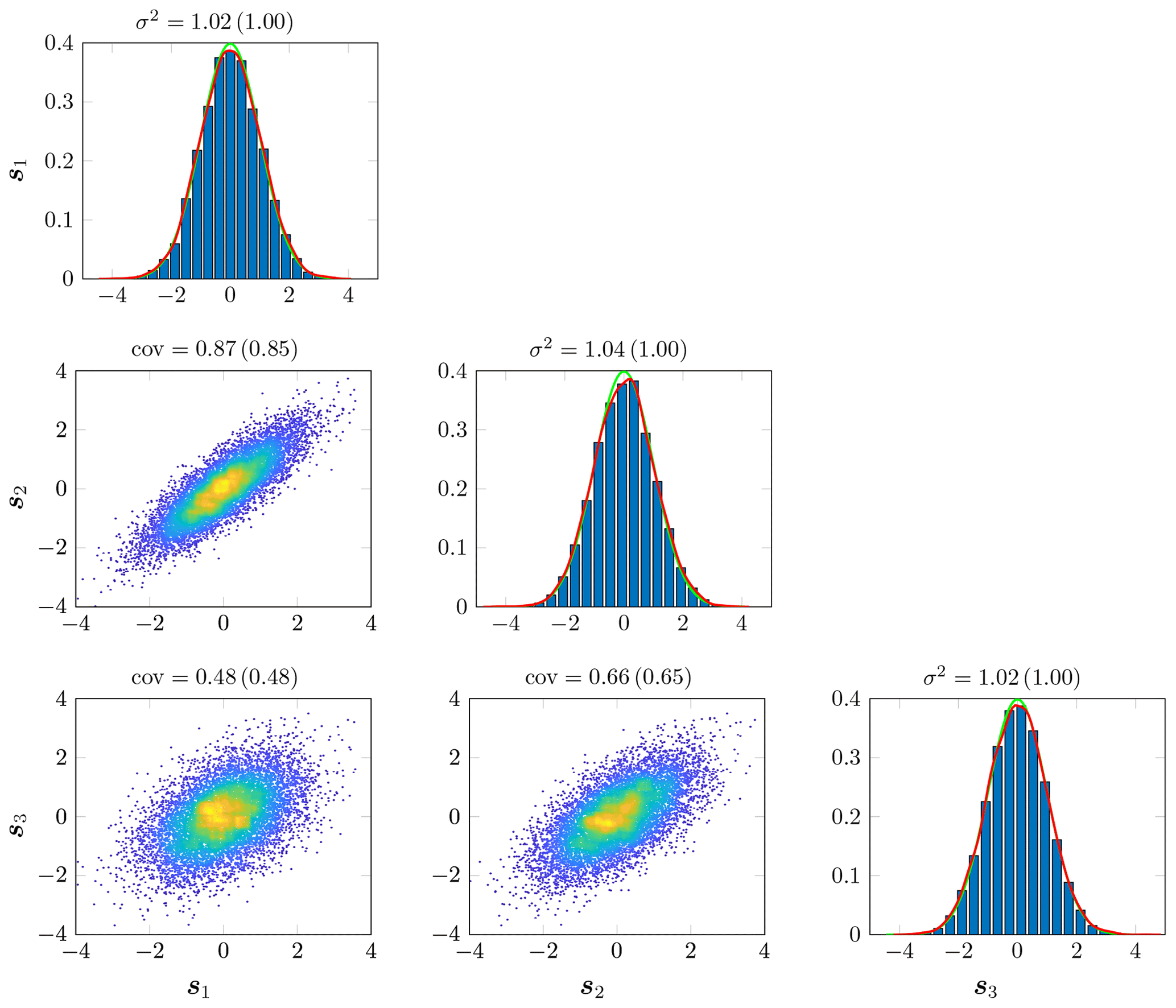
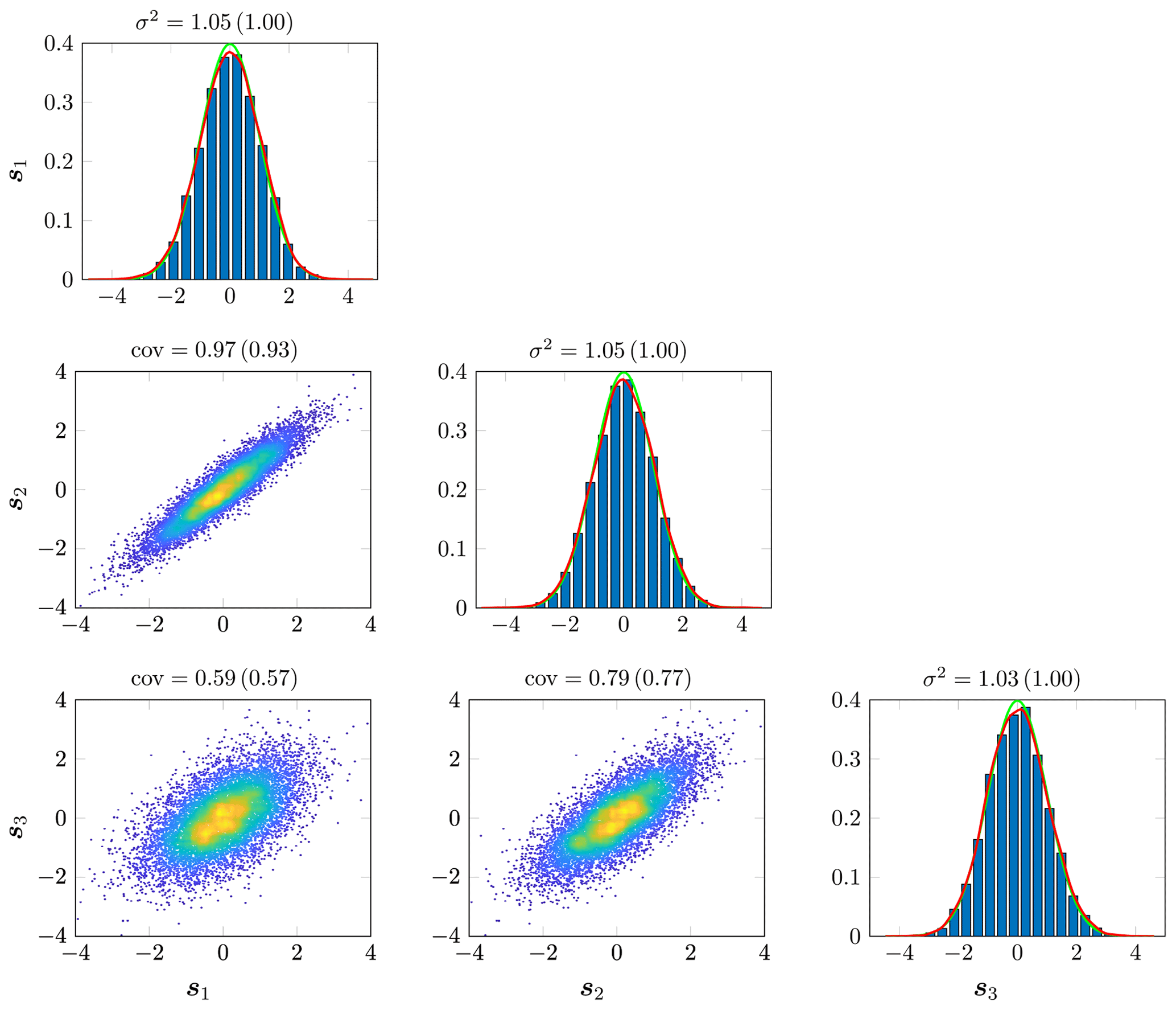
Figure 1 Estimated marginal and bivariate distributions of the samples generated by solving the SPDE (Eq. 2) with α=2. Estimates are based on 10 000 samples. Results are shown for the locations ${\mathit{s}}_{\mathrm{1}}=(\mathrm{50},\mathrm{50})$ km, ${\mathit{s}}_{\mathrm{2}}=(\mathrm{53.125},\mathrm{50})$ km and ${\mathit{s}}_{\mathrm{3}}=(\mathrm{59.375},\mathrm{50})$ km. The estimated covariances and variances are also provided with the theoretical values determined from Eq. (1) shown in parentheses. For the marginal distributions, the red curves represent the kernel density estimates and the green curves are standard Gaussian distributions.

Figure 2 The same as Fig. 1 but for α=4.

3.1 Experiment 1: verification of covariance structure

As a first experiment, we test our implementation by checking that the generated samples are actually drawn from a Gaussian random field with the desired Matérn covariance function. More specifically, the marginal distributions have to follow Gaussian distributions with zero mean and unit variance, while the bivariate distributions have to follow bivariate Gaussian distributions with zero mean and covariance given by Eq. (1). To test for the covariance structure, we generate an ensemble of 10 000 independent and identically distributed (i.i.d) samples and estimate the marginal and bivariate distributions from these samples. Figures 1 and 2 show the obtained distributions for the locations ${\mathit{s}}_{\mathrm{1}}=(\mathrm{50},\mathrm{50})$ km, ${\mathit{s}}_{\mathrm{2}}=(\mathrm{53.125},\mathrm{50})$ km and ${\mathit{s}}_{\mathrm{3}}=(\mathrm{59.375},\mathrm{50})$ km for α=2 and α=4, respectively. In both figures, we observe that the marginal and bivariate distributions all follow a Gaussian distribution with variances and covariances close to the theoretical expected values. Small discrepancies between the estimated variances and covariances and their theoretical values can be explained by the numerical approximations (finite-element discretization and lumped approximations), the impact of boundary conditions (discussed in Experiment 2), and the limited number of samples used for the estimation.

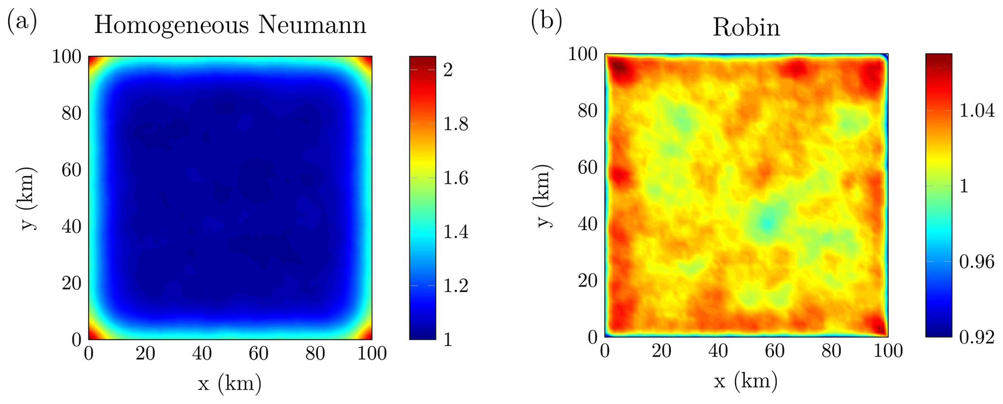
Figure 3 Comparison of estimated marginal standard deviations with homogeneous Neumann boundary conditions (a) and Robin boundary conditions (b) with the Robin coefficient given by $\mathit{\beta }=\left(\mathit{\kappa }\mathit{\tau }\right)/\mathrm{1.42}$.

3.2 Experiment 2: influence of the boundary conditions

The second experiment investigates the influence of the boundary conditions on the marginal variance of the samples generated following the SPDE approach. Figure 3 shows the estimated marginal standard deviation for α=2 with 10 000 samples considering either homogeneous Neumann boundary conditions (Fig. 3a) or Robin boundary conditions (Fig. 3b). The value of the Robin coefficient β is taken as $\mathit{\kappa }\mathit{\tau }/\mathrm{1.42}$. With homogeneous Neumann boundary conditions, we observe a clear boundary artefact that yields a larger marginal standard deviation close to the boundary than in the interior. In particular, the standard deviation is 1.4 times larger along the edges of the domain and 2 times larger near the corners. The boundary artefact becomes almost negligible near a distance of at least ρ from the boundary. On the contrary, Robin boundary conditions with an appropriate choice of the Robin coefficient help mitigate the boundary artefact significantly. Physically, Neumann boundary conditions can be interpreted as reflecting boundaries, while Robin boundary conditions can be understood as absorbing boundaries, with the Robin coefficient being an absorption coefficient.

Figure 4 Estimated autocorrelation functions (dotted lines) for different values of the temporal correlation factor ϕ as a function of the temporal lag T. Solid lines represent the theoretical autocorrelation functions given by Eq. (17).

3.3 Experiment 3: transient simulation

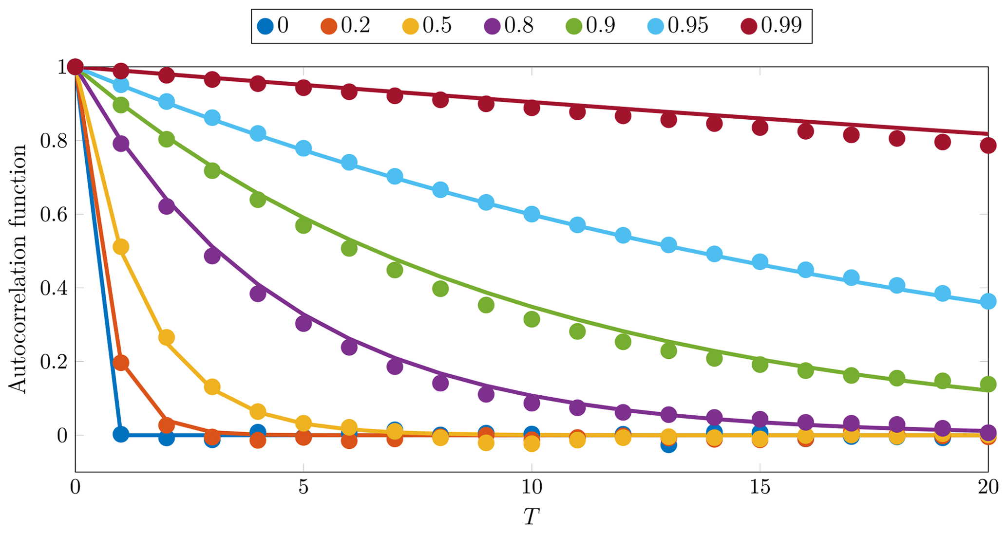
As a third experiment, we test our transient implementation by checking that the generated samples follow an AR1 process in time. For different values of the temporal correlation factor ϕ, we generate a series of 10 000 spatio-temporal samples and estimate the autocorrelation function at the centre location $\mathit{s}=(\mathrm{50},\mathrm{50})$ km. Figure 4 represents the estimated autocorrelation functions and provides a comparison with the theoretical autocorrelation functions given by Eq. (17). For all temporal correlation factors, the estimated autocorrelation functions are close to their theoretical value. The small discrepancies can also be explained by numerical approximations and the limited number of samples in the time series.

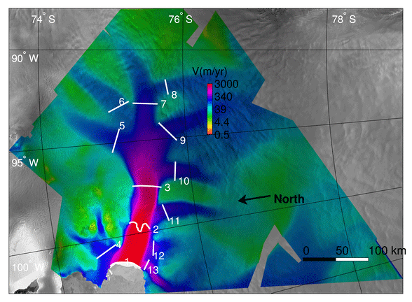
Figure 5 Fluxgates used to compute mass fluxes on tributaries of the PIG. Each gate is numbered from 1 to 13 and corresponds to one tributary. Gate 1 coincides with the ice front, and gate 2 coincides with the 1996 grounding line. The gates are superimposed on an InSAR surface velocity map of the area, in logarithmic scale (Rignot, 2008). Image is taken from Larour et al. (2012b), courtesy of the Journal of Geophysical Research: Earth Surface.

4 Stochastic sampler: application

4.1 Experimental setup

We set up a test problem similar to the application in Larour et al. (2012b), in which the authors performed a UQ analysis on the Pine Island Glacier using a partitioning approach. We refer the reader to this article for additional information about the ice flow model, the datasets, the input quantities, and the quantities of interest. We consider three spatially varying uncertain input quantities: the ice thickness H, the basal drag coefficient α at the ice–bed interface and the ice hardness B. The basal drag coefficient is used in a Budd-type friction law, and the ice hardness is determined from a thermal model (Larour et al., 2012c). As quantities of interest, we consider the mass flux through 13 fluxgates positioned along the main tributaries of the PIG (see Fig. 5). The mass flux M_i through gate i is given by

$$\begin{array}{}\text{(18)}& M_i=\underset{{\mathcal{C}}_i}{\int }{\mathit{\rho }}_{\text{ice}}H\mathit{v}\cdot \mathit{n}\mathrm{d}l,\end{array}$$

where the integral is a line integral along the fluxgate contour 𝒞_i, v is the depth-averaged horizontal velocity computed using the shallow shelf/stream approximation (SSA) (MacAyeal, 1989), n the downstream unit normal vector to the fluxgate contour and ρ_ice the ice density. All 13 mass fluxes are computed simultaneously for each forward run of ISSM and each sample of the input quantities.

The anisotropic mesh used in this application comprises 2085 elements and 1112 nodes, with higher spatial resolution near the shear margins and the grounding line. The number of nodes is sufficiently small to make both the sampling (tenths of a second per sample) and the solving of the ice-sheet model (a few seconds per run) computationally fast.

4.2 Characterization of uncertainty

Following Larour et al. (2012b), we perturb each input quantity with a multiplicative noise proportional to a local (measurement) error margin. More specifically, we represent each source of uncertainty in the following way:

$$\begin{array}{}\text{(19)}& q\left(\mathit{s}\right)=q_{\text{ref}}\left(\mathit{s}\right)(\mathrm{1}+{\mathit{\sigma }}_q(\mathit{s}\left)p_q\right(\mathit{s}\left)\right),\end{array}$$

where q_ref is a reference value for each source of uncertainty, σ_q is the (spatially distributed) error margin for each source of uncertainty and p_q(s) is a spatially distributed random perturbation. The reference thickness value is derived from bedrock topography (Nitsche et al., 2007) and surface elevation (Bamber et al., 2009; Griggs and Bamber, 2009) data. The temperature-dependent reference ice hardness value is derived from an Arrhenius law (Larour et al., 2012c) and surface temperature data by Comiso (2000). The reference basal drag coefficient is inferred using an inverse method (Morlighem et al., 2010) with the reference thickness and ice hardness values. For the UQ analysis in Sect. 4.3 and 4.4, we only perturb the ice thickness, and the error margins are based on ground-penetrating radar (GPR) cross-over measurements from the 2009 Operation IceBridge Campaign and provided by the Center for Remote Sensing of Ice Sheets (CReSIS); see also Larour et al. (2012b) for further information. For the sensitivity analysis in Sect. 4.5, we specify a spatially uniform 5 % error margin for all three inputs to compare sensitivities between input variables with same error margins.

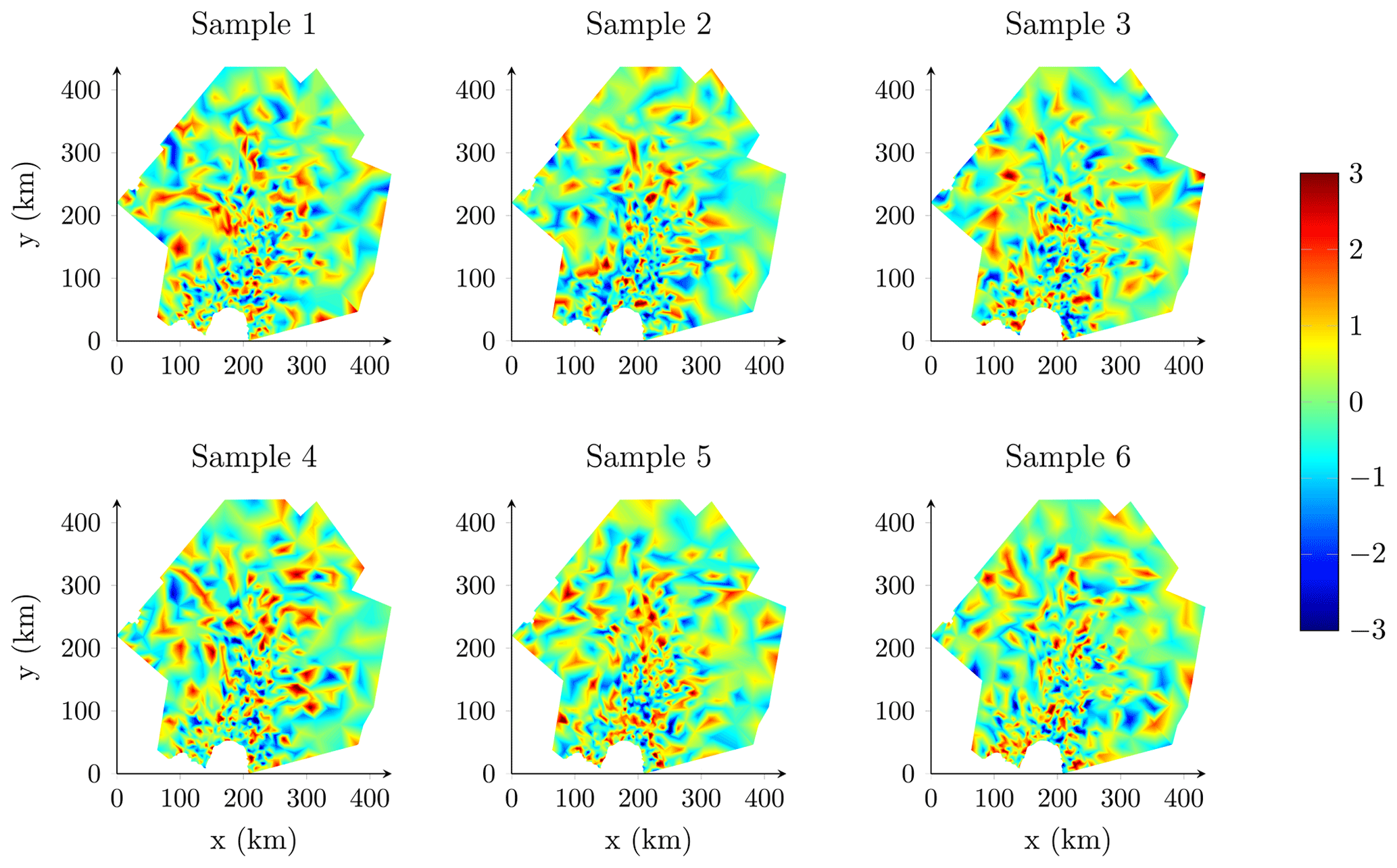
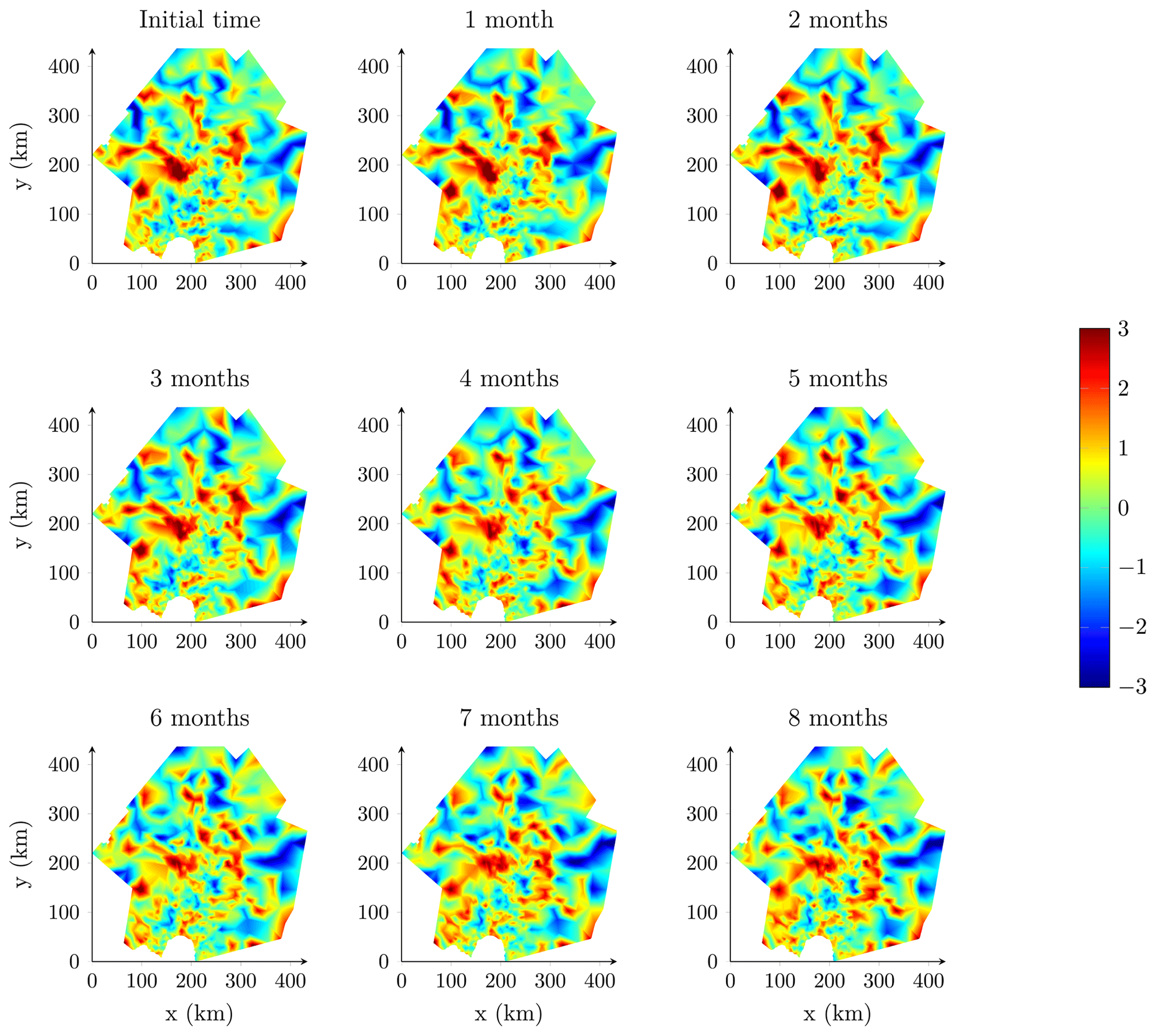
Figure 6 Samples of the random perturbation p_q(s) over Pine Island Glacier with a parameter range of 10 km.

Figure 7 The same as Fig. 6 but with a parameter range of 30 km. For comparison, the SPDE (Eq. 2) is solved with the same realizations of the right-hand side as in Fig. 6.

Figure 8 The same as Fig. 6 but with a parameter range of 100 km. For comparison, the SPDE (Eq. 2) is solved with the same realizations of the right-hand side as in Fig. 6.

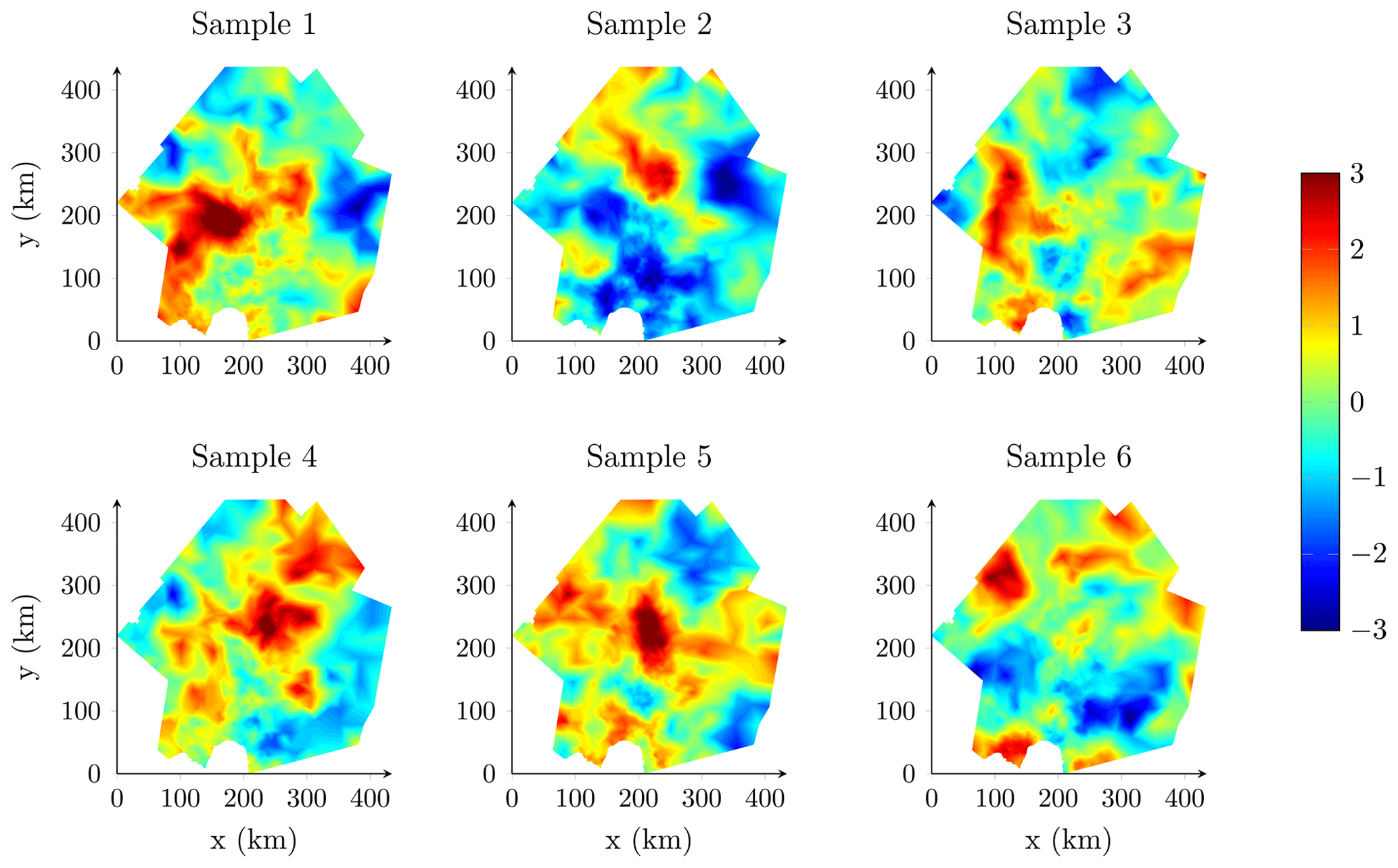
Here, we represent the random perturbation p_q as a Gaussian random field with Matérn covariance function and unit variance (σ²=1) following the SPDE approach. Therefore, each uncertain input quantity is represented as a Gaussian random field with mean q_ref, Matérn covariance function and marginal standard deviation proportional to q_ref(s)σ_q(s). We solve the SPDE (Eq. 2) for α=2 and impose Robin boundary conditions with $\mathit{\beta }=\left(\mathit{\kappa }\mathit{\tau }\right)/\mathrm{1.42}$. We consider different parameter ranges ρ to investigate the impact of the spatial correlation on the results. The parameters κ and τ are determined from Eqs. (3a)–(3c). As an illustration, we represent samples of the random perturbation for ρ = 10 km in Fig. 6, ρ = 30 km in Fig. 7 and ρ = 100 km in Fig. 8. For this application, we have chosen the values of the parameter range arbitrarily without any proper data assimilation or inversion process. The use of an unconstrained parameter range is justified by the fact that we do not seek to provide new probabilistic mass balance estimates for the Pine Island Glacier but seek only to demonstrate the interest of the implemented stochastic sampler for forward UQ analysis.

4.3 Propagation of uncertainty

We use ISSM to propagate uncertainty in ice thickness into a probabilistic characterization of the depth-averaged mass flux across fluxgates. We implement the propagation of uncertainty using Monte Carlo sampling. To this end, we begin by generating an ensemble of n i.i.d samples of the random perturbation by solving the stochastic equation (Eq. 2) for an ensemble of n i.i.d samples of the random right-hand side 𝒲(s). Following this, we run the ISSM computational model for each sample of the input variable to generate an ensemble of n i.i.d samples of the depth-averaged mass flux across the 13 fluxgates. From these samples, we can estimate the mean and standard deviation of the mass flux across the fluxgates with the statistical mean and standard deviation of the samples. In addition, we can estimate the probability density distribution of the mass flux across the fluxgates by using a normalized histogram of the samples or kernel density estimation (Scott, 2015). In all of our simulations, we found that n=2500 samples were sufficient to ensure reasonably converged statistical estimates (bootstrap error of a few hundredths of a percent for the mean and a few percent for the standard deviation).

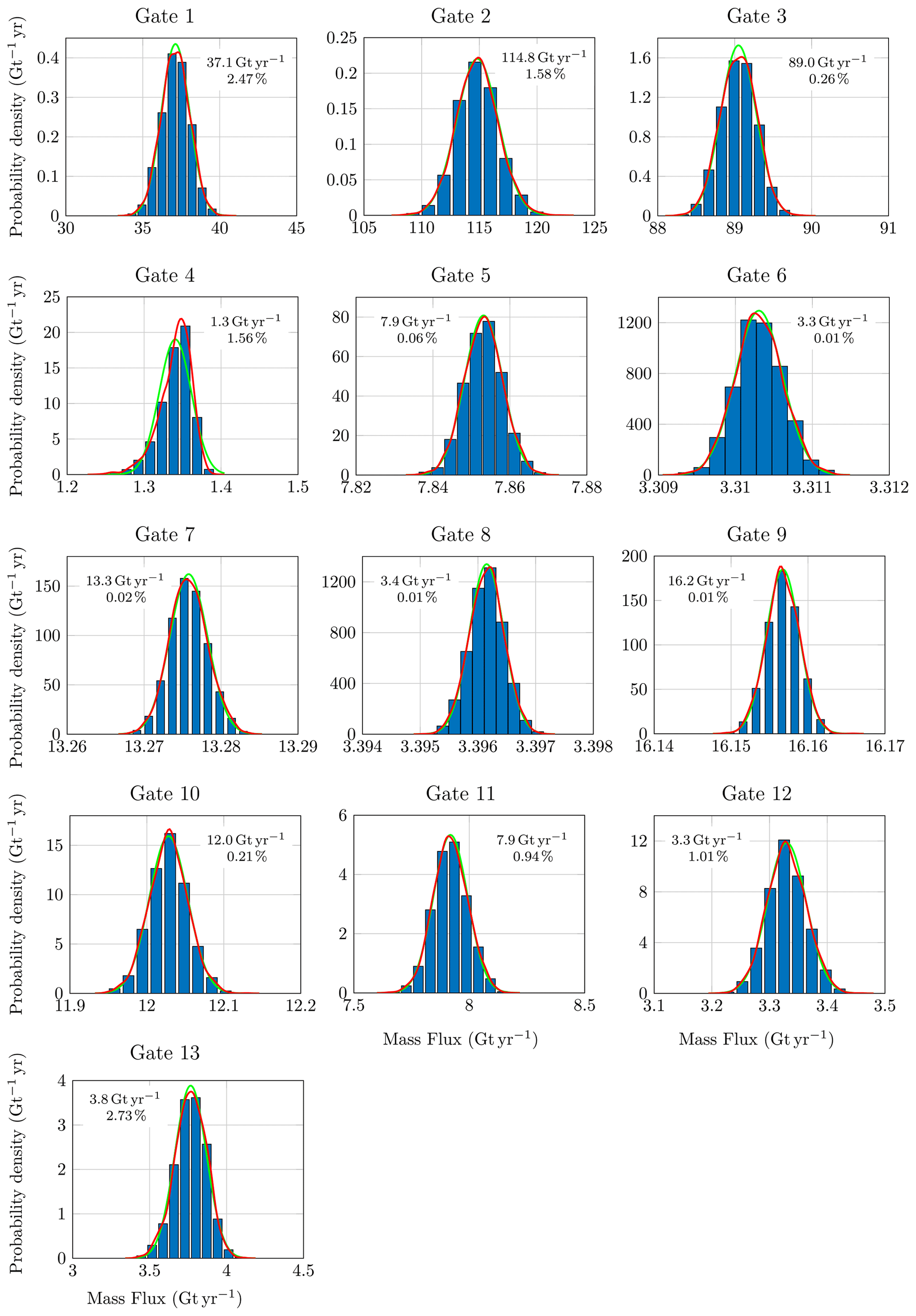
Figure 9 Normalized histograms for the mass flux across the fluxgates depicted in Fig. 5. The mean (in Gt yr⁻¹) and the coefficient of variation (in percent) are provided for each gate. The kernel density estimate of the probability density function is shown in red, and its Gaussian approximation with corresponding mean and coefficient of variation is shown in green. Results are obtained for a parameter range of 30 km.

Figure 9 shows, for a parameter range of 30 km, the statistical distribution of mass flux through each gate as a normalized histogram of the samples, along with a kernel density estimate of their probability density function. The estimated mean and coefficient of variation (defined as the standard deviation over the mean) are also provided. The statistical distribution of mass flux through each gate can be considered Gaussian (which can be checked formally by carrying out a Kolmogorov–Smirnov test), with the exception of gate 4, for which the distribution is negatively skewed. The estimated mean values are approximately equal to the mass fluxes obtained for the reference ice thickness. The coefficients of variation range from of a few hundredths of percent to a few percent, with the fluxgates close to the ice front exhibiting the largest uncertainty. As already shown in Larour et al. (2012b), the mass flux response to input uncertainties is particularly smooth.

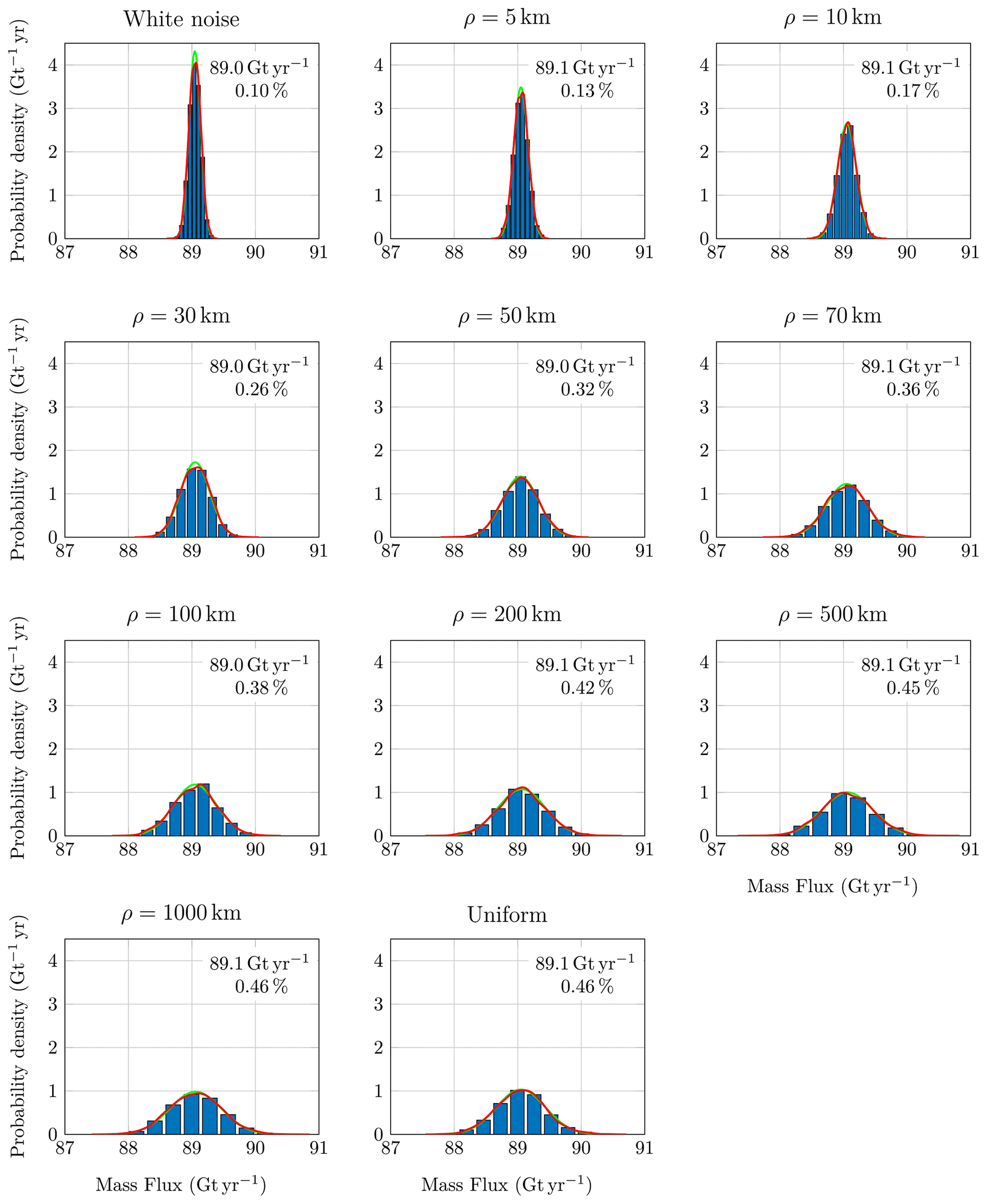
Figure 10 Normalized histograms for mass flux across fluxgate 3 (see Fig. 5) for different parameter ranges. The mean μ (in Gt yr⁻¹) and the coefficient of covariation are provided for each parameter range. The kernel density estimate of the probability density function is shown in red, and its Gaussian approximation with corresponding mean and coefficient of variation is shown in green.

Figure 10 shows the statistical distribution of mass flux through gate 3 for different parameter ranges ρ. We also present results for a white noise perturbation (zero correlation length) and a uniform Gaussian perturbation (infinite correlation length). We observe that the mean value does not depend on the parameter range while the overall uncertainty (measured as the coefficient of variation) increases with the parameter range. With the exception of gate 4, similar conclusions can be drawn for all the other gates. The specific behaviour of gate 4 may result from the non-Gaussianity of the mass flux distribution, and the coefficient of variation is not the most appropriate measure of dispersion for skewed distributions.

4.4 Sensitivity analysis to ice thickness changes

We carry out a global sensitivity analysis to determine where changes in ice thickness most influence uncertainty in mass flux across fluxgates. For a given fluxgate, we can build a sensitivity map which gives for each location a sensitivity measure (or index) between the random field at this location and the mass flux across the fluxgate. Here, we consider the coefficient of correlation between the random field and the mass flux M_i as a sensitivity measure, i.e.

$$\begin{array}{}\text{(20)}& {\displaystyle \frac{\text{Cov}\left(p_q\right(\mathit{s}),M_i)}{\sqrt{\mathbb{V}\left[p_q\right(\mathit{s}\left)\right]\mathbb{V}\left[M_i\right]}}},\end{array}$$

where Cov denotes the covariance between two random variables and 𝕍 denotes the variance. We mention that other sensitivity measures like the Spearman's or Kendall rank correlations, the distance correlation sensitivity index, or the Hilbert–Schmidt independence criterion sensitivity index (Da Veiga, 2014; De Lozzo and Marrel, 2016) can also be considered as long as these indices can handle dependent variables.

Figure 11 Sensitivity map (visual representation of the coefficient of correlation) for mass flux across fluxgates depicted in Fig. 5. Results are for a parameter range of 30 km.

Figure 11 shows a sensitivity map for the mass flux through each gate for a parameter range of 30 km. The coefficients of correlation are estimated from the 2500 samples obtained in Sect. 4.3. A positive (negative) index value indicates a positive (negative) linear correlation between changes in ice thickness and changes in mass flux across a fluxgate, and a zero value indicates no linear correlation. As expected, only a limited region on the glacier has a significant influence on the mass flux across a given fluxgate. This region is usually concentrated close to the fluxgate, though more remote locations can have an influence, as can be seen for instance with fluxgates 6, 7 and 9. These remote locations lie in the main ice stream of the PIG, thus suggesting that uncertainty in ice thickness in the main ice stream can impact ice flow in upstream tributaries. With the exception of gate 4, sensitivity maps show a positive (linear) correlation between changes in ice thickness and changes in mass flux across fluxgates.

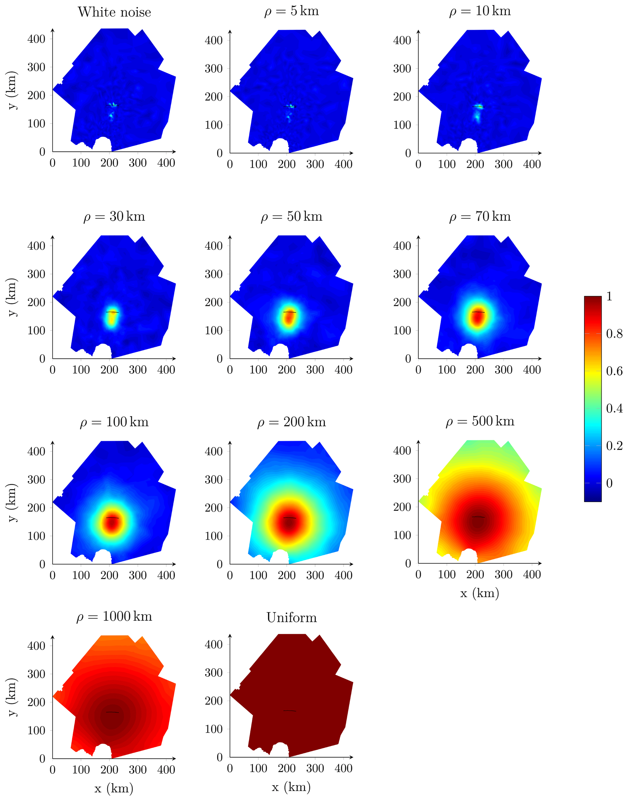
Figure 12 Sensitivity map (visual representation of the coefficient of correlation) for mass flux across fluxgate 3 (see Fig. 5) for different parameter ranges.

Figure 12 shows a sensitivity map of mass flux through gate 3 for different parameter ranges and white noise and uniform perturbations. As expected, increasing the parameter range expands the zone of influence and the magnitude of the correlation. Therefore, the larger the correlation length, the further away from the gate uncertainties in ice thickness can influence mass flux estimates.

4.5 Sensitivity analysis to multiple input quantities

We perform another sensitivity analysis by considering multiple sources of uncertainty, namely uncertainty in ice thickness, basal friction and ice hardness. We assume that these three sources of uncertainty are statistically independent, and we choose a parameter range of 30 km for all of them. Because the sources of uncertainty are statistically independent, we can use the Sobol or variance-based sensitivity indices (Sobol', 2001; Saltelli et al., 2008) to characterize the contribution of each source of uncertainty to the uncertainty in the mass flux across each fluxgate. The first-order Sobol index S_i,j measuring the contribution of the random field $\left\{x_i\left(\mathit{s}\right),\mathit{s}\in D\right\}$ to the uncertainty in the mass flux M_j is defined as

$$\begin{array}{}\text{(21)}& S_{i,j}={\displaystyle \frac{\mathbb{V}\left[\mathbb{E}\right[M_j\left|\left\{x_i\left(\mathit{s}\right),\mathit{s}\in D\right\}\right]]}{\mathbb{V}\left[M_j\right]}}.\end{array}$$

The Sobol index of a given uncertain input parameter represents the fraction of the variance of the projections explained as stemming from this sole uncertain parameter. A value of 1 indicates that the entire variance of the projections is explained by this sole uncertain parameter, and a value of 0 indicates that the uncertain parameter has no impact on the projection uncertainty. We estimate these Sobol indices using Monte Carlo sampling following the estimation method by Janon et al. (2014). We use a total of ν=4 × 5000 evaluations of the computational model to estimate the Sobol indices.

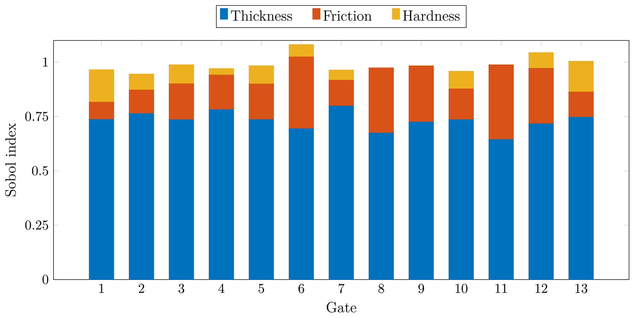
Figure 13 Sobol sensitivity indices for the mass flux across flux gates. The gap between the height of a bar and the unit value represents the interaction index.

Figure 13 shows the Sobol sensitivity indices for each gate. Though the sum of all three sensitivity indices should be less than 1, the sum of the estimated indices exceeds this value for a few gates (gates 6, 12 and 13). This suggests that the Sobol estimates are not totally converged for some gates. From Fig. 13, we find that the uncertainty in the ice thickness has the largest influence on the uncertainty in the mass flux across fluxgates, accounting for more than 60 % to 80 % of their variance. The second most influential input parameter is the basal friction coefficient (Sobol indices ranging from 5 % to 35 %), except for gates 1 and 13 lying on the ice shelf where there is no basal friction.

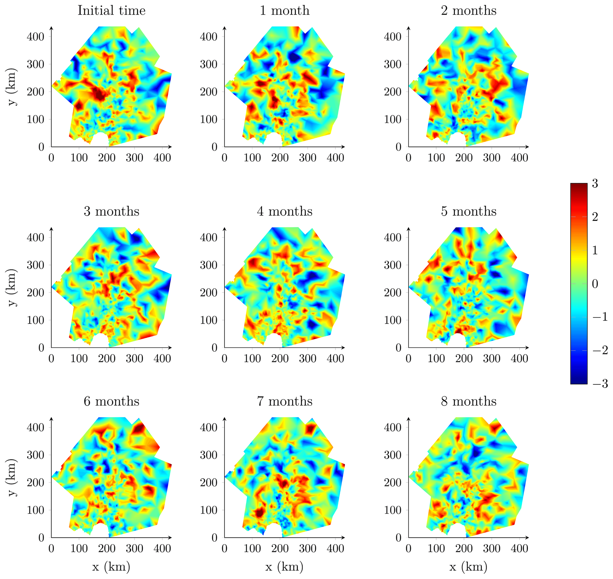
Figure 14 Transient samples of random perturbation over Pine Island Glacier with a temporal correlation of 0.5.

Figure 15 The same as Fig. 14 but with a temporal correlation of 0.95. Figures 14 and 15 have the state initial state.

4.6 Transient analysis

Finally, we present a transient experiment of the Pine Island Glacier over a 10-year period. The Pine Island Glacier is forced by basal melting underneath the floating portion of the domain and surface mass balance. We impose a basal melting rate of 25 m yr⁻¹, and we consider the surface mass balance (smb) to be uncertain. We represent the uncertain smb as

$$\begin{array}{}\text{(22)}& \text{smb}(\mathit{s},t)={\text{smb}}_{\text{ref}}\left(\mathit{s}\right)(\mathrm{1}+{\mathit{\sigma }}_{\text{smb}}{p}_{\text{smb}}(\mathit{s},t\left)\right),\end{array}$$

where smb_ref is a reference value for the smb taken from Vaughan et al. (1999), σ_smb is a constant 10 % error margin and p_smb(s,t) a spatio-temporal random perturbation. The spatio-temporal random perturbation is represented as a spatio-temporal Gaussian random field given by Eq. (16). The spatial noise has a parameter range of 30 km. We assume that the smb exhibits a temporal monthly variability, and consequently we discretize the temporal process in time with a 1-month time step. We use the same time step to run the ISSM model forward in time. Figures 14 and 15 show two realizations of the random perturbation for a temporal correlation of 0.5 and 0.95, respectively.

Figure 16 Normalized histograms for mass flux across fluxgate 3 (see Fig. 5) as a function of time. The mean (in Gt yr⁻¹) and the coefficient of variation (in percent) are provided for each time. The kernel density estimate of the probability density function is shown in red, and its Gaussian approximation with corresponding mean and coefficient of variation is shown in green. Results are for a parameter range of 30 km and a temporal correlation of 0.5.

Figure 16 shows the statistical distribution of mass flux through gate 3 as a function of time for a temporal correlation of 0.5. We observe an increase in the mean mass flux through the gate due mainly to the ocean forcing, with the estimated mean values approximately equal to the mass flux in the absence of stochastic smb forcing. Most gates show an increase in their mean mass flux in time, except for gate 4, which shows a decrease in its mean mass flux, and gates 2, 8, 9 and 13, which show a relatively constant mean mass flux in time. However, we observe an increase in the coefficient of variation of the mass flux for all gates, thus suggesting that mass balance estimates become increasingly uncertain in time.

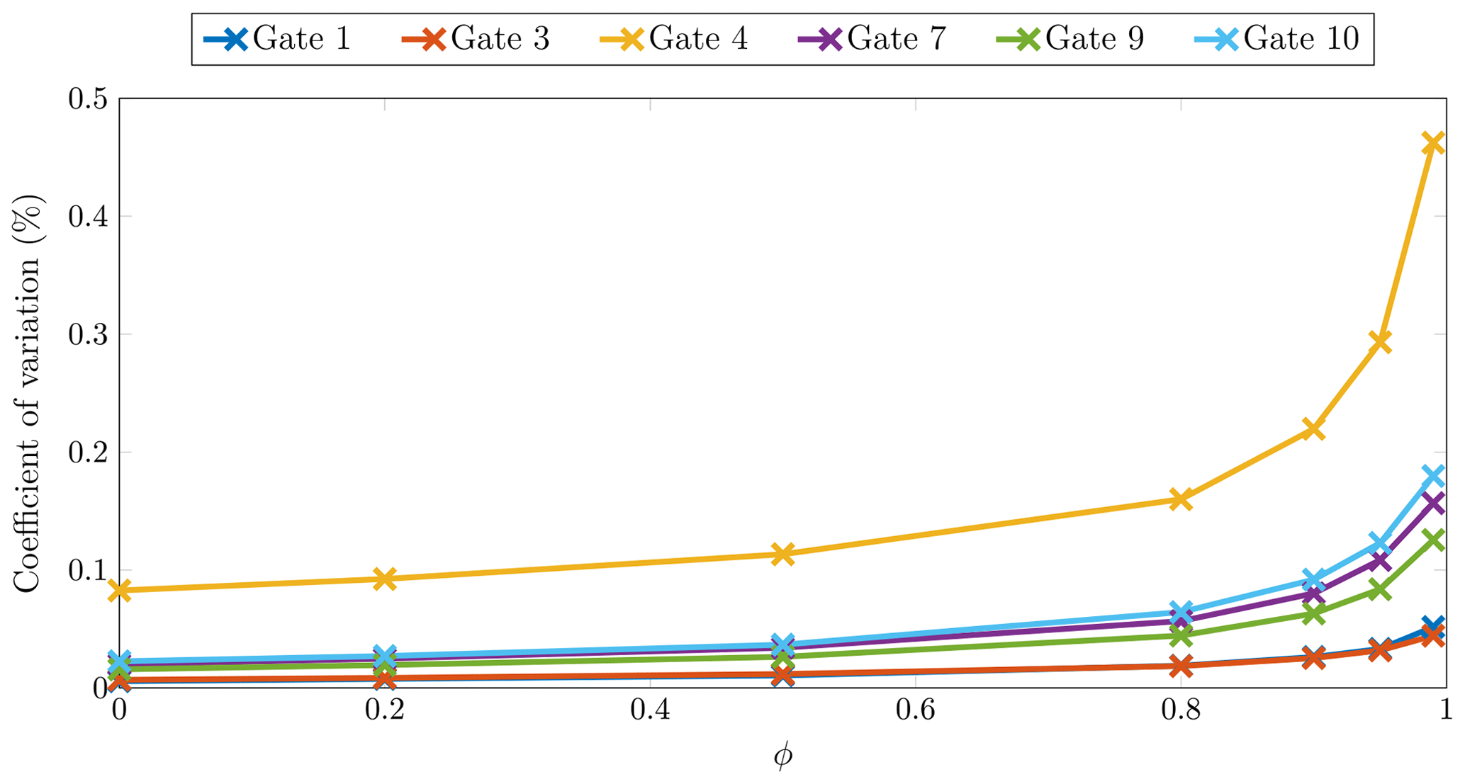
Figure 17 Coefficient of variation at the end of the simulation as a function of the temporal correlation ϕ. Results are for different gates.

Figure 17 shows the coefficient of variation at the end of the simulation as a function of the temporal correlation ϕ for a few gates. From this figure, it is clear that increased temporal correlation results in increased uncertainty in the mass flux, with a more significant increase for higher values of the temporal correlation.

5 Discussion

Model-based projections of ice-sheet mass balance should all be ideally given in the form of probabilistic projections that provide an assessment of the impact of uncertainties in boundary conditions, climate forcing, ice sheet geometry or initial conditions. In this context, uncertainty quantification analysis with ice-sheet models should capture the spatial and temporal variability of these sources of uncertainties. To this end, random fields are an essential statistical tool for the modelling and analysis of uncertain spatio-temporal processes. Here, we take advantage of the explicit link between Gaussian random fields with Matérn covariance function and a stochastic partial differential equation to implement a random field sampler within ISSM. The FEM-oriented implementation of ISSM and its fully object-oriented and highly parallelized architecture allow for a straightforward and computationally efficient implementation of this SPDE. This stochastic sampler provides an alternative to the pre-existing UQ mesh partitioning approach implemented within the ISSM-DAKOTA UQ framework. The partitioning approach can be interpreted as the representation of a random field with perfect correlation for locations in a same partition and zero (Larour et al., 2012b) or non-zero correlation (Larour et al., 2020) for locations in different partitions. Because the partitions are constant throughout the sampling, realizations strongly depend on the partitioning, which is not the case with the stochastic sampler we implemented. In the partitioning approach, the number of partitions artificially controls the spatial scale of the random perturbation. In contrast, spatial correlation is an intrinsic feature of Gaussian Matérn random fields and can be controlled through the parameter range ρ. In addition, random samples generated following the SPDE approach are mesh independent as long as the mesh resolution is sufficiently fine to capture the desired spatial variability.

The results presented here provide complementary insight into the impact of uncertainties on the PIG. First, our results are consistent with previous results by Larour et al. (2012b) showing that the SSA model is stable to uncertainties in ice thickness. For most gates, the probability distribution of the mass flux can be considered as a Gaussian distribution centred around the reference value. The overall uncertainty is relatively small and does not exceed a few percent of the mean value at most. This suggests that the response of the PIG to changes in ice thickness is relatively smooth even if the ice flow dynamics is non-linear. Therefore, robust projections of mass balance estimates of the PIG are possible even in the presence of uncertainties in ice thickness. Second, our results show that a higher spatial correlation length results in larger uncertainty in mass balance estimates. The correlation length controls the size of the region around each gate in which changes in ice thickness significantly impact mass flux through the gates (see Fig. 12). This conclusion is consistent with Schlegel et al. (2018), who showed that many small partitions would likely underestimate uncertainty in model outputs while the use of a single partition would likely overestimate the uncertainty. Third, our sensitivity analysis shows that ice thickness is the most influential parameter in inducing uncertainty in mass flux estimates. Although this conclusion is consistent with Larour et al. (2012b), both conclusions cannot be directly compared because we carried out a global sensitivity analysis rather than the local sensitivity analysis performed in the latter study. A local sensitivity analysis measures the sensitivity of the mass flux to local changes in input data and assumes that each input variable is independent. This hypothesis is not appropriate for correlated random fields. In contrast, the global sensitivity analysis in Sect. 4.5 allows us to consider the global uncertainty in the random field and only requires the different random fields to be statistically independent. Fourth, our transient simulation shows that uncertainty in mass balance estimates increases in time and for higher temporal correlations.

Finally, we discuss a few limitations of the SPDE approach. First, this approach relies on the assumption that uncertainty in spatially varying input parameters can be appropriately characterized by a Gaussian random field. Though Gaussian random fields are a practical model for many stochastic phenomena, this assumption may not be appropriate because input parameters can have an asymmetric distribution or heavy tails or can simply be positive or bounded. While this may sound restrictive, non-Gaussian random fields can be obtained through non-linear transformations of Gaussian random fields (Vio et al., 2001; Hristopulos, 2020) or by solving the SPDE with a non-Gaussian white noise (Bolin, 2014). Second, representing spatio-temporal processes with a separable autoregressive model relies on the assumption that the spatial and temporal variabilities are uncoupled and that the temporal variability can be simply described with a first-order Markov process. These two assumptions may be too restrictive to describe the complex spatio-temporal variability of stochastic processes like the surface mass balance (White et al., 2019). Third, the SPDE and autoregressive models require the specification of model parameters, most notably the spatial and temporal correlation lengths. As shown in Sect. 4, these parameters have a major impact on the uncertainty in mass balance estimates. Therefore, these parameters should ideally be constrained through data assimilation methods, modelling efforts, and inverse methods, including Bayesian inference; see, for instance Cameletti et al. (2012) and Western et al. (2020), for Bayesian spatio-temporal inference with hidden Gaussian random fields. Lastly, we assumed the spatial correlation to be constant on the PIG. While this assumption might seem reasonable for a single glacier, this may be more questionable for an ice sheet with different drainage basins. However, this issue may be handled by considering a spatially varying parameter κ, as already discussed in Sect. 2.1.1.

6 Conclusions

We presented and implemented a Gaussian random field sampler within ISSM for uncertainty quantification analysis of spatially (and temporally) varying uncertain input parameters in ice-sheet models. So far, sampling of spatially varying uncertain input parameters within ISSM has relied on a partitioning of the computational domain and sampling from the partitions. This approach may be limited in representing spatial and temporal correlations. To improve the probabilistic characterization of spatially (and temporally) correlated uncertain input parameters, we proposed to generate realizations of Gaussian random fields with Matérn covariance function. Our implementation relies on an explicit link between Gaussian random fields with Matérn covariance function and a stochastic partial differential equation. This SPDE sampling approach allows for a computationally efficient sampling of random fields using the FEM and provides a flexible mathematical framework to build probabilistic models of spatio-temporal uncertain processes. In addition, model parameters allow us to intrinsically control the spatial and temporal correlations of the realizations and their variance and smoothness.

We applied this stochastic sampler to investigate the impact of spatially (and temporally) varying sources of uncertainties, namely uncertainties in ice thickness, basal friction, ice hardness and surface mass balance, on the Pine Island Glacier. More specifically, we investigated the impact of spatial and temporal correlations on ice-sheet mass balance. We showed that the SSA model is stable to uncertainties. We also showed that larger correlation lengths lead to increased uncertainty in mass balance estimates because the random perturbations have a larger length scale of influence. We found that the most influential source of uncertainties for estimating mass balance is the uncertainty in ice thickness. We also showed in a transient experiment that uncertainty in mass balance estimates increases in time and with higher temporal correlation. Overall, our results demonstrate the need to better constrain the spatial and temporal variability of physical processes impacting ice-sheet dynamics through data assimilation and modelling efforts.