Computation of backwater effects in surface waters of lowland catchments including control structures – an efficient and re-usable method implemented in the hydrological open-source model Kalypso-NA (4.0)

Backwater effects in surface water streams and on adjacent lowland areas caused by mostly complex drainage and flow control structures are not directly computed with hydrological approaches yet. A solution to this weakness in hydrological modelling is presented in this article. The developed method enables transfer of discharges into water levels and calculation of backwater volume routing along streams and adjacent lowland areas by balancing water level slopes. The implemented and evaluated method extends the application of hydrological models for rainfall–runoff simulations of backwater-affected catchments with the advantages of (1) modelling complex flow control systems in tidal backwater-affected lowlands, (2) less effort to parameterise river streams, (3) directly defined input factors of driving forces (climate change and urbanisation) and (4) runtime reduction of 1 to 2 orders of magnitude in comparison to coupled hydrodynamic models. The developed method is implemented in the open-source rainfall–runoff model Kalypso-NA (4.0). Evaluation results show the applicability of the model for simulating rainfall–runoff regimes and backwater effects in an exemplary lowland catchment (Hamburg, Germany) with a complex flow control system and where the drainage is influenced by a tidal range of about 4 m. The proposed method is applicable to answer a wide scope of hydrological and water management questions, e.g. water balances, flood forecasts and effectiveness of flood mitigation measures. It is re-usable to other hydrological numerical models, which apply conceptual hydrological flood-routing approaches (e.g. Muskingum–Cunge or Kalinin–Miljukov).

1 Introduction

There is open demand in hydrological modelling of rainfall–runoff regimes in backwater-affected lowlands. The flow routing in lowland catchments is characterised by artificially drained catchments using manifold flow control structures. The occurrence of backwater effects in such complex lowland river streams and on adjacent lowland areas poses an open research question in hydrological modelling. Adjacent lowland areas in this article are distinguished by a low ground level and connection to rivers. The size of lowlands varies from narrow riparian areas, to wetlands, shallow retention spaces, floodplains, and vast partly urbanised marshlands or swamplands. Hydrological models are applied to simulate processes in the compartments of the (1) surface–atmosphere interaction, (2) the transition between soil–vegetation–atmosphere, (3) the processes in the vadose zone of the soil and (4) the flood routing in the receiving surface waters. In lowlands, the last two issues require more detailed considerations because of mostly high groundwater levels and the drainage against fast-changing water levels in tidal streams of complex flow control systems. For simulating the interaction between groundwater and surface water quite a few approaches are available (Brauer et al., 2014; Waseem et al., 2020; Sun et al., 2016). However, modelling backwater effects in tidal streams with fast-changing water levels in complex flow control systems of lowland catchments directly with hydrological models has not been implemented in most hydrological approaches up to now (Waseem et al., 2020).

Simulating backwater effects, velocity fields and the spatial distribution of water depths for flood inundation maps demands 2D or 3D hydrodynamic–numerical models with the numerical integration of the partial differential equations describing the flood-routing processes. To compute spatial detailed simulation results in river streams and floodplains, coupled hydrological and hydrodynamic model approaches fit well in terms of meeting the required modelling objectives. But, hydrodynamic–numerical models require larger effort to parameterise river streams and simulation times, which are at least 1 to 2 orders of magnitudes longer in comparison to conceptual hydrological flood-routing approaches to model river streams. High-resolution data describing the topography of the main channel and the natural floodplain in the case of bank overflow are necessary. Hence, the availability of suitable detailed profile data from measurements is significant for hydrodynamic–numerical modelling. The larger effort in data resources and runtime for hydrodynamic–numerical model simulations is no limitation for answering special research questions and creating detailed inundation maps. However, applying a coupled hydrological–hydrodynamic model shows disadvantages in the application on mesoscales to regional catchment scales (>100 km²) and for operational forecast applications. Therefore, it is proposed in this article that a stand-alone hydrological approach can be beneficial in flood forecasting models to enable parsimonious and efficient modelling of flood-routing and backwater effects in lowlands by a conceptual hydrological method producing less detailed results.

The demand to solve this weakness in hydrological numerical models is increasing, since in low-lying tidal catchments, the pressure on current storm-water flow control systems is rising due to combined impacts of enlarged urbanisation on the one hand and climate-change-induced sea level rise in combination with heavy storm events on the other hand (IPCC, 2013, 2014; UN DESA, 2018). Studies about the combined risk of high tides (storms) and storm-water events are given by Lian et al. (2013), Nehlsen (2017), Klijn et al. (2012), Zeeberg (2009), Huong and Pathirana (2013), and Sweet et al. (2017). These selected examples all show conformity about the tendency that lowlands will be faced by higher pressures to mitigate flooding in the future. A promising flood mitigation measure against the effects of (high) precipitation events in low-lying catchments is the controlled temporary storage of water in retention areas. However, state-of-the-art hydrologic approaches reveal shortcomings in modelling the flood-routing and retention volume in backwater-affected lowland catchments.

1.1 Objectives

To resolve the previously described shortcomings in hydrological approaches to model the flood routing in backwater-affected lowland catchments five objectives are defined. The method shall be (1) applicable to model complex flow control systems in backwater-affected lowlands, (2) efficient by using short runtimes for real-time operational model application, (3) open for further model developments, (4) re-useable for other hydrological model solutions and (5) parsimonious with regard to the complexity of input parameters. Reaching a balance between model structure details (namely complexity) and data availability is an important issue to keep the model as parsimonious and efficient in runtime as possible, but complex enough to explain the heterogeneity in the areas and the dynamics in the hydrological processes. To accomplish the five defined objectives for a re-usable, open, efficient and parsimonious hydrological method to model backwater effects, the authors suggest developing a conceptual extension approach for state-of-the-art flood-routing methods (for instance, Muskingum–Cunge or Kalinin–Miljukov).

1.2 Outline

The literature review in Sect. 2 discusses current weaknesses in hydrological models to simulate backwater effects and subsequent flooding of adjacent lowland areas. The theoretical concept in Sect. 3 and the developed method in Sect. 4 explain the worked-out solution. The implementation of the methodology is realised in the open-source hydrological model Kalypso-NA version 4.0 (Sect. 5). The evaluation of the method is done using observed data for an exemplary lowland catchment study in Hamburg, Germany, where a complex drainage system and backwater-affected streams have a significant impact on the flow regime (Sect. 6). A discussion of results points out the main findings and limitations in Sect. 7. The article closes in Sect. 8 with a summary and an outlook on follow-up research.

2 State of the art in hydrological modelling to compute flood-routing and backwater effects in lowlands

Flood routing describes the processes of translation and retention of a flood wave moving along a stream in the downstream direction. To simulate the flood routing in rivers different approaches are applied: (1) pure black box (namely empirical, lumped), (2) hydrological conceptual or (3) hydrodynamic–numerical approaches (Maniak, 2016; Hingray et al., 2014). The applicable flood-routing method needs to be chosen with respect to the modelling purpose and available data. Computation of water depths and backwater effects in rivers as well as on forelands by using hydrological approaches (1 and 2) is rarely done and up to now has mostly been linked with comparatively high uncertainties. The missing applicability of hydrological approaches for simulating backwater effects is shown in a recent study within the North German lowlands (Waseem et al., 2020).

Commonly applied conceptual hydrological approaches are described e.g. in Todini (1991) with the indicated year of publication: storage routing as presented by Puls (in 1928), Muskingum or Muskingum–Cunge routing described by McCarthy (in 1938) and Cunge (in 1969), and Kalinin and Miljukov routing (in 1958) or linear reservoir and channel cascade routing presented by Maddaus (in 1969). The purpose of hydrological flood-routing approaches is to compute the discharge hydrographs in the considered stream segments. For hydrological approaches, conceptual or empirical parameters are calibrated based on observed events like in the frequently used Muskingum method. A compromise involves hydrological methods using profile data on streams to model the flood routing, for example in the Muskingum–Cunge approach and the approach of Kalinin and Miljukov. These concepts use profile information in a conceptual way and require far less calculating effort for mesoscale modelling (>100 km²) than hydrodynamic–numerical approaches.

Only a few related studies are available with respect to modelling backwater effects in mesoscale catchments with hydrological approaches, while none of the reviewed studies enabled the computation of backwater retention in lowland areas for mitigating backwater-induced flooding. Coupled hydrological–hydrodynamic computation models like in MIKE SHE coupled with MIKE 11 (Waseem et al., 2020) or in the German Model NASIM coupled with a hydrodynamic computation model (Loch and Rothe, 2014; Dorp et al., 2017) are not part of this comparison because of the previously described disadvantages in hydrodynamic approaches. A focus is set on direct or stand-alone hydrological model enhancements.

In Waseem et al. (2020), a review of models is published with regard to simulating important hydrological processes in coastal lowlands. This review shows weaknesses in SWIM (soil- and water-integrated model) and HSPF (hydrological simulation program Fortran). The approaches in the models SWAT (soil and water assessment tool) and MIKE SHE show good conformity to simulate processes in lowlands, while both are not applicable to model backwater effects in the river, on floodplains, or in other adjacent lowlands as well as backwater effects caused by control structures (sluices, pumping stations and tide gates). An enhanced approach in SWAT for riparian wetlands (SWATrw) is presented in Rahman et al. (2016) to compute the surface water interaction between river streams and explicitly defined wetlands, while backwater effects in streams are unconsidered. The modified SWAT-Landscape Unit (SWAT-LU) model enables the computation of horizontal hydraulic interactions between a river and the aquifer beneath the adjacent floodplain (Sun et al., 2016). Similarly, in the rainfall–runoff model WALRUS (Wageningen Lowland Runoff Simulator) a lumped approach is realised to model the following processes: (1) groundwater–unsaturated zone coupling, (2) groundwater–surface water feedbacks, and (3) seepage and surface water supply (Brauer et al., 2014). These are important model features to model the runoff regime in lowlands, but neither of the approaches enables the computation of backwater effects (1) along streams, (2) among stream sections and the land surface, and (3) in river sections influenced by upstream of control structures.

More nation-specific studies to model backwater effects in streams are done with the German model ArcEGMO (by the Büro für Angewandte Hydrologie, Berlin). The hydrological model ArcEGMO takes into account backwater effects by hindering the downstream flood routing when the water level at the downstream segment is higher than the upstream one (Pfützner, 2018). The method presented by the National Hydrological Forecasting Service (NHFS) in Hungary (Szilagyi and Laurinyecz, 2014) applies a discrete linear cascade model to account for backwater effects in flood routing by adjusting a storage coefficient of the cascade. The ArcEGMO and NHFS methods calculate a retained flood routing, but neither computes backwater volume being routed into upstream segments by a reverse flow direction or the backwater-induced flooding of adjacent lowland areas.

In a study by Messal (2000), backwater effects among river streams and the subsurface flow in riverbanks are modelled exemplarily for the catchment Stör (1157 km²) in Schleswig-Holstein, Germany. Messal applies a proportional relationship between upstream and downstream elements for calibration purposes. The model serves well for the catchment study Stör, but the parameter values are non-transferable to other catchments because of a lack of physical descriptions.

Another approach is presented by Riedel (2004) to model the backwater effects among river streams in German lowlands for the example of two tidal tributaries of the Weser River. The approach uses the reservoir cascade theory including the input parameters of the roughness coefficient by Manning–Strickler and geometric descriptions of the profiles for the flood-routing computation. The river is modelled as a cascade of reservoirs (namely a NASH cascade), while the water level from the previous time step of the downstream segments is taken into account to compute the flood routing. A time step shift in the computational approach is accepted by Riedel (2004) because he reduced the simulation time step size to 1 min. The model computes a reservoir cascade on the basis of a defined boundary condition at the downstream segment. However, the explicit simulation of backwater-induced flooding of flood prone areas or adjacent lowland areas is not included.

These reviewed hydrological methods compute backwater effects in a more or less conceptual way with the described weaknesses and limitations. None of these studies analysed the backwater-induced flooding of lowland areas or, in this specific case, retention areas. Consequently, none of the studies accomplish simulation of a controlled retention of backwater volume in such areas, subsequent drainage or the hydrological processes influenced by backwater-induced flooding. Further on, most studies do not apply physically based parameters to transfer validated values and knowledge from one catchment to other studies. A methodology to solve these shortcomings is proposed in this article.

3 Theoretical approach to enhance a hydrologic conceptual flood-routing method to compute backwater effects

To reach the described objectives, a state-of-the art conceptual hydrological method is extended to be applicable for the computation of backwater effects in streams and adjacent lowland areas (incl. retention areas). This section describes the theory of the conventional hydrological approaches to compute the flood routing (Sect. 3.1), the concept of modelling control structures in tidal lowlands (Sect. 3.2), and the approach to compute backwater effects with a conceptual hydrological approach in streams and adjacent lowland areas (Sect. 3.3).

3.1 Conceptual hydrological flood-routing approach

State-of-the-art hydrological flood-routing theory in free-flow conditions describes the flood wave propagation in streams which are not affected by downstream conditions. This means that an afflux in front of obstacles downstream of the considered stream segment is assumed to have no impact on the upstream segments. With this assumption, backwater effects are not considered. Flood-routing processes depend on the characteristics of the drainage network comprising the geometry of profiles, gradients and roughness of the streams. Linear or non-linear Muskingum approaches have no physically based parameterisation and require input parameters which are based on observed data in upstream and downstream segments of rivers. Therefore, these hydrological approaches are not suitable for simulation with changed geometries or changed flow conditions in streams where no observed data are available. This lack is solved in two approaches, which are based on physical characteristics such as river geometry, stream length, roughness coefficient and riverbed slope. On the one hand, the Muskingum–Cunge (often used in the United States) is applicable, and on the other hand, the Kalinin–Miljukov (KM) flood-routing approach is applicable. For this work, the approach of Kalinin–Miljukov is chosen, since this approach is widely applied in Germany and eastern Europe.

The approach of Kalinin and Miljukov (1957) (KM approach) divides a stream into a number of characteristic lengths. Each length is considered to be short enough for assuming a quasi-stationary relationship on the basis of a hysteresis curve. Different derivations of the KM approach are given in the literature and discussed, for example, by Koussis (2009). More details about the applied approach in this work are explained in the Supplement, Sect. S4.

With such conceptual hydrological flood-routing approaches the magnitude and time of flow along a stream on the basis of stream characteristics are determined. They describe the (free-flow) propagation of discharge through streams, whereby translation and retention processes along the stream change the shape of the hydrograph from an upstream to a downstream point. The explicit direction of computation from upstream to downstream restrains the modelling of backwater effects. This means that backwater effects caused by an afflux are ignored in these conceptual hydrological approaches, and an extension is therefore developed in this article (see Sect. 3.3).

3.2 Concept to model control structures in lowland catchments

Backwater effects in river sections are often caused at obstacles like weirs, (tide) gates, and retention or detention reservoirs, which also function as control structures in streams. It is required to model these structures in hydrological models since such control structures are regularly used to control the flow in catchments. In this article, we focus on control structures frequently applied in lowland drainage areas. Operation rules of control structures are mostly pre-defined depending on operative criteria. The criteria are normally based on thresholds of water level, discharge or precipitation intensity within hindcasted or forecasted data (see Fig. 1). Since the data time series influence the status of control structures, they are defined in this article as drivers. There is a difference between pre-set and on-the-fly processed driver data. Pre-set data time series are imported such as observed water level or precipitation data. Additionally, data series which are computed during runtime (e.g. discharge) can likewise serve as drivers and are processed on the fly.

Figure 1 (a) Illustration of operative criteria in a control function depending on driver time series of precipitation, water level and discharge. (b) Scheme of a control structure with a control function changing the water level W(t), volume V(t) or outflow Q(t) per time step t.

When a threshold of an operative criterion is reached during the runtime of the model, the status of the system is changed (e.g. opening or closing a gate). The change in the status based on reached thresholds is described in control functions, which are checked per time step. In a control structure the retained water can cause backwater effects in the upstream direction if an afflux of water occurs. Control structures are one component type within a hydrological network. Other component types are streams (linear data structures), areas (spatial data structures) and nodes (point data structures). An explanation of these components of a hydrological network is given in the Supplement (Sect. S3).

3.3 Concept of the flood-routing enhancement to compute backwater effects

The previously described hydrological conceptual approach (here, of Kalinin and Miljukov) is enhanced by using the resulting water level, volume and discharge (WVQ) relation to compute backwater effects per stream element. The concept enables the computation of a backwater volume routing according to the water level slope. This is illustrated in a scheme in Fig. 2 for a river longitudinal segment which is separated in several strands. At the downstream segment a control structure is located. In stage (1) the free flood routing in the downstream direction is computed. When the barrier (e.g. a tide gate) is closed by control functions (stage 2), an afflux of water is generated (stage 3). The afflux initiates a “backwater volume routing” (stage 4), meaning that the water volume is routed in the upstream direction to equalise the surplus water level of the afflux. When the barrier is opened, the backed-up water volume is routed downstream (stage 5). These five stages are computed according to the water level slope in each time step. The methodology to realise the coding of this theoretical concept into a numerical hydrological model is explained in Sect. 4.

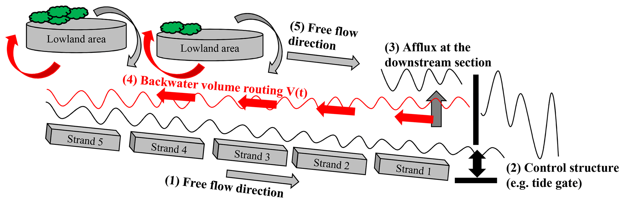
Figure 2 Scheme of five computation steps in the developed concept to compute backwater effects with a hydrological approach: (1) free-flood-routing computation downstream, (2) control structure simulation, (3) afflux computation, (4) backwater-volume-routing computation in the upstream direction including adjacent lowland areas (as well as retention areas) and (5) free-flood-routing computation after opening the barrier.

4 Methodology to compute backwater effects in rivers and adjacent lowland areas with complex flow control systems

The methodology to calculate backwater effects with a hydrological conceptual approach consists of three main algorithms: a transfer of discharges to water levels and volumes per stream segment and time step (Sect. 4.1), the calculation of (inter)active control structures (Sect. 4.2), and a backwater volume routing according to the water level slope along stream segments and adjacent lowland areas (Sect. 4.3).

4.1 Transfer of discharges to water levels and volumes

The flood routing in stream segments of the hydrological network is computed with conceptual hydrological approaches like Kalinin–Miljukov or Muskingum–Cunge (see Sect. 3.1). A transfer of discharges into water levels and volumes is done by calculating the flow regimes using the approaches of Manning–Strickler or Darcy–Weisbach.

According to the Kalinin–Miljukov approach, each stream segment is divided into a cascade of n reservoirs with a characteristic length L_c and the coefficient K_c. The WVQ relations for different states (n_WVQ) in the stream segment are defined with an interpolation between supporting points of water level heights. This results in a division of the bankfull water level height H_full (m a.s.l.) into (n_WVQ) states with a water level difference ΔH (m). Three calculation routines are integrated in the flood-routing method to compute the flow velocity in stream segments. The appropriate calculation routine is selected according to the stream segment's profile and data availability. Stream segments with a circular profile are computed with the Darcy–Weisbach approach and the flood-routing method of Euler (1983). Stream segments with rectangular or trapezoidal (angular) profiles are likewise computed with the Darcy–Weisbach or with the Manning–Strickler approach. The equivalent sand roughness k_s (m) using the Darcy–Weisbach approach and the roughness K_st (m${}^{\mathrm{1}/\mathrm{3}}$ s⁻¹) using the Manning–Strickler approach are input parameters. The algorithm of these three calculation routines is illustrated in the flowchart in Fig. 3. The Fortran code and equations to compute the following list of flood-routing parameters are explained in the Supplement, Sect. S4: flow velocity v, characteristic lengths L_KM, number of characteristic reservoirs n_KM, retention parameters K_KM, water levels W, volumes V and discharges Q, where KM indicates the parameter calculation according to the Kalinin–Miljukov approach.

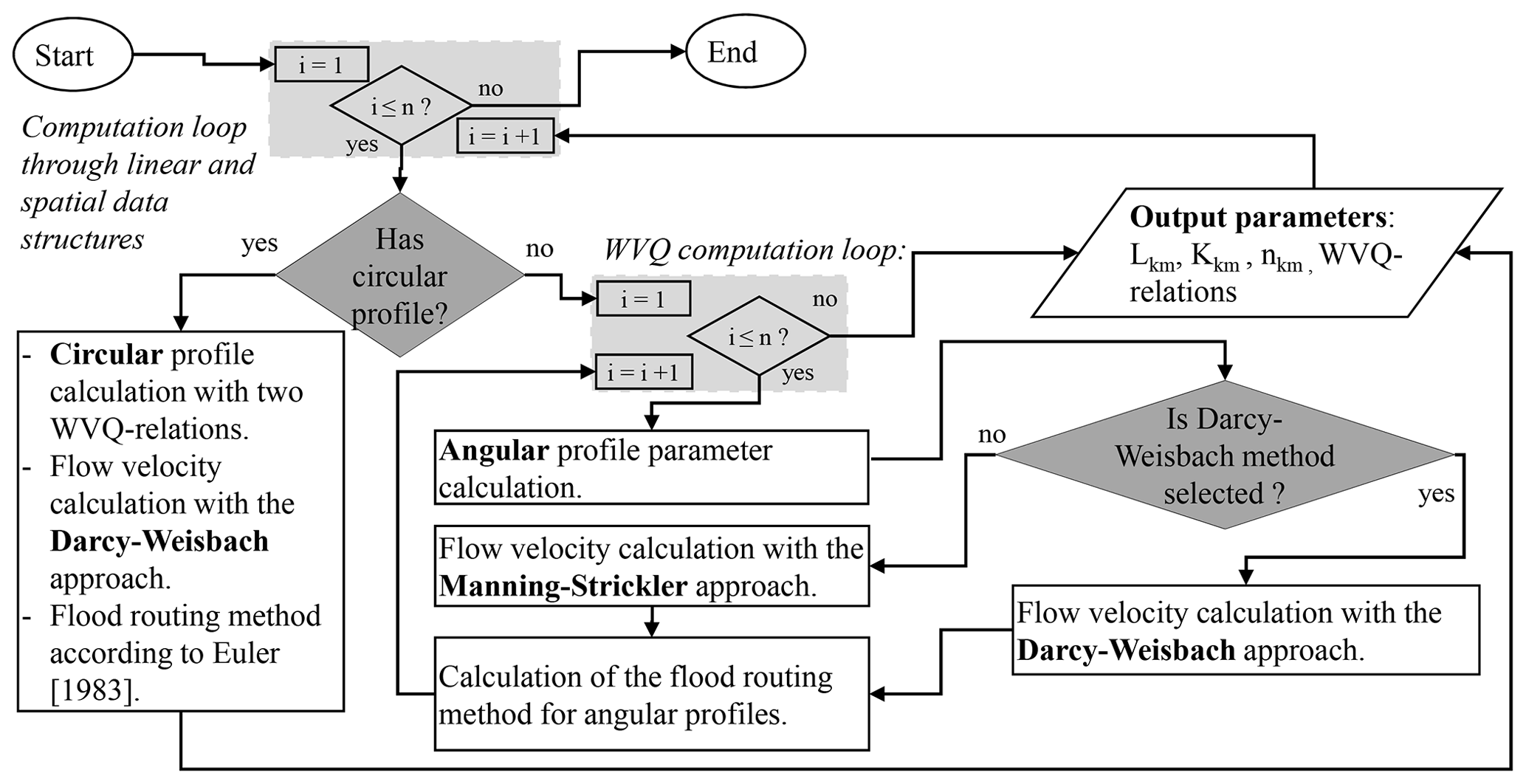
Figure 3 Algorithm to compute the relations between water level, volume and discharge (WVQ) per stream segment.

4.2 Calculating (interactive) control functions of drainage systems

A control structure of a linear stream segment is defined with unsteady WVQ relations, and the flood routing is modelled with a storage indication method. In this work the modified Puls method is applied. The outflow of the control structure can be distributed to four receivers (Fig. 4). Operative criteria of control structures are defined for three types of driver time series, which are precipitation intensity, water level stages and discharge values. Hydrographs of water level stages and discharges are results given at junction nodes, while precipitation time series are related to sub-catchments as spatial input data. The status of control structures is checked per time step during the execution of the numerical model. A differentiation of control function types is done according to their operative criteria depending on pre-set (externally pre-processed), on-the-fly (internally processed) or interactive on-the-fly driver time series. The three control function types and the dependency on the location of the operative criteria are listed in Fig. 4. Control function type (1) depends on observed or externally forecasted driver time series, for instance precipitation intensity or water level gauge data. These control functions are computed in the pre-processing phase of the simulation run to set the status of a control structure. With forecasted data a time duration can be set to change the status of control functions (closing or opening a gate) with a specific lead time before the threshold (operative criteria) is reached. In the control function type (2), criteria depend on the output of computed parameters of the hydrological network, namely water level or discharge. The functions are computed during the simulation run on the fly. This procedure depends on the condition that the driver elements are located upstream of the control structure and are not influenced by backwater. If the criteria of a control structure depend on downstream or backwater-affected conditions in an interactive system, a recursive calculation routine is started to compute the control function type (3). The recursive calculation routine is explained in Sect. 4.3.

Figure 4 Scheme of a control structure with discharge distribution functions to four receivers and the three control function types depending on operative criteria.

4.3 Calculating backwater effects along river streams and adjacent lowland areas

An afflux due to natural or artificial obstructions (for instance, gates or weirs) leads to a rise of water level in upstream segments. To simulate the resulting backwater effects, the downstream-directed surplus water volume is reversed as backwater when the downstream water level is higher than upstream. This concept is illustrated in the theoretical approach in Sect. 3.3 and comprises the simulation of backwater effects, which cause the flooding of upstream lowland areas. The developed algorithm to compute these backwater effects is illustrated in the flowchart in Fig. 5. The calculation routines are nested in computational loops as follows: a spatial loop of streams and areas is nested in a time loop. The time loop is again nested in a backwater system loop.

Figure 5 Algorithm to compute backwater effects in streams and lowland areas (like retention areas) with the indicated calculation routines (a, b, c, d). It is realised with a space-before-time algorithm for modelling backwater effects and control structures per backwater system.

Each backwater system includes several component types of a hydrological network: linear structures (stream segments), spatial structures (sub-catchments of lowland areas), junction nodes and a control structure (tide gate or water level gauge) at the downstream segment. For the control functions type (1) and type (2) (see Sect. 4.2) the calculation routines (a) to (c) in Fig. 5 are executed, while at any element an afflux condition is present (see query “Is backwater system active?” = yes). Additionally, per backwater system (j) and per time step (t) a query checks if an interactive backwater system with a control function type (3) is defined. An interactive system depends on both downstream and upstream conditions. In the case of an interactive system, the flag for a “recalculation” loop is activated. The final balanced stage is reached when in a backwater-affected system the downstream water levels are not higher than the upstream water levels within a range of a minimum “tolerated” water level difference. The method demands the definition of a minimum difference (ΔW_min) according to the application purposes. A smaller tolerated water level difference increases the accuracy of computed water level results. At the same time, this increases the number of backwater computational runs ($k=k+\mathrm{1}$) before reaching a maximum number (currently: k=10 000). This critical state prevents infinite calculation routines and a warning shows if this limit is reached to check the input parameters, which include an adjustment of the tolerated water level difference. In the exemplary evaluation study (see Sect. 6), a water level difference of about ΔW_min=0.01 m gives sufficient results for mesoscale stream segments. For local-scale stream segments a difference of about ΔW_min=0.001 m gives adequate results (Hellmers, 2020). Backwater effects are computed in open stream segments and adjacent lowland areas which are part of the defined backwater system. For intermediate closed circular profiles having a limited storage capacity, the backwater volume is routed upstream to the next open stream segment.

In the calculation routine a (Fig. 5), the initialisation of formal parameters of each linear and spatial data structure for the backwater effect computation is performed. This includes an initialisation of the water level, volume and discharge per time step. Discharges are computed with the flood-routing approaches described in Sect. 3.1. The corresponding water levels and retained water volumes are derived from the calculated WVQ relations per stream segment (see Sect. 4.1). The initialisation of the parameters for the backwater effect computation is illustrated in Fig. 6. For the computation of backwater effects, the formal parameters of each linear and spatial data structure are initialised. This includes an initialisation of the water level, volume and discharge per time step. Discharges are computed with the flood-routing approaches described in the Supplement Sect. S3. The corresponding water levels and retained water volumes are derived from the calculated WVQ relations per stream segment. When the volume in the control structure is increased ($V\left(t\right)>V(t-\mathrm{1})$), afflux is generated and the flag for afflux conditions is set to “true”. The difference in volume between time steps (ΔV(t−1)h) is revised continuously during the following backwater calculation routines (b) and (c) (Fig. 5). When the volume in the control system is decreased ($V\left(t\right)<V(t-\mathrm{1})$) or not changed ($V\left(t\right)=V(t-\mathrm{1})$) the flag for afflux conditions is set to “false” and the volume (ΔV(t−1)) is reduced by the proportion of the changed volume ΔV, which has already been processed in the time step before. The upstream-directed backwater routing is computed if the afflux conditions flag is set to true. The downstream-directed backwater routing is computed if the afflux conditions flag is set to false.

In the calculation routine b (Fig. 5), the backwater effect computational loop in the upstream direction is activated, while afflux conditions are present in the backwater system. The calculation is done per stream segment in a computational loop starting at the downstream element (i=n). If the difference in water levels between the current and the upstream segment is larger than the defined tolerated water level difference ΔW_min, an algorithm to compute the backwater effect is activated. The backwater quantity derived from an afflux at the downstream segment is routed to the upstream segments. Along the streams, spatial structures (like lowland catchments) are linked where the water is retained or causes backwater flooding. This developed concept is illustrated in the scheme in Fig. 7, where the backwater effect computation between stream segments with linked spatial structures (retention areas) is shown. The formal parameters of the WVQ relations of the current (i) and the upstream (i−1) segment are processed. The computation is done in three sub-calculation routines (namely A, B and C) to compute the water level and volume stages.

Explanation of the sub-calculation routine (A): in the case of adjacent lowland areas (linked spatial data structures), a portion of water flows from the stream segment (i) into the respective linked areas (i) if the water level exceeds the riverbank. The inflow continues until the water level in the stream W_i(t) is in balance with the water level in the linked spatial data structures W_i,areas(t). The result is a decreased difference in volume ΔV_i(t) to be routed to the upstream segment (i−1) per time step.

Explanation of the sub-calculation routines (B) and (C): the computed backwater effect in the calculation routine (B) describes how the water volume ΔV_i(t) is added to the upstream linear data structure ${V^{\prime }}_{i-\mathrm{1}}\left(t\right)=V_{i-\mathrm{1}}\left(t\right)+\mathrm{\Delta }V\left(t\right)$, whereupon the water level is derived from the WVQ relations. If the upstream segment is linked with another spatial data structure as illustrated in Fig. 7 (case C), the balancing of water level and volume is done according to the procedure in (A). As long as a backwater effect is present in any river segment or adjacent lowland area, the calculation is repeated (until k=10 000). The algorithm to compute upstream-directed backwater effects on the water levels and volumes is illustrated in Fig. 8. If the following queries are true, the upstream backwater effect computation is executed. These queries are called at the beginning of the calculation routine (see “Are afflux conditions present?”) with the following equation:

$$\begin{array}{}\text{(1)}& \text{is }{W}_i\left(t\right)-W_{i-\mathrm{1}}\left(t\right)>\mathrm{\Delta }{W}_{\min }\text{? and is }{V}_i\left(t\right)>V_{i,\mathrm{free}}\left(t\right)\text{?},\end{array}$$

where the water level W_i(t) (m a.s.l.) and volume V_i(t) (m³) are defined by the WVQ relation per stream segment with the index (i). ΔW_min(t) is the tolerable backwater-affected water level rise given for the stream segments (m) in the backwater system. V_i,free(t) is the water volume in the segment without backwater effects, which is computed with the flood-routing method. While afflux conditions are present, the water level in the current stream segment (i) is reduced by the minimum water level difference ΔW_min(t). The adjusted storage volume of the stream segment ${V^{\prime }}_i\left(t\right)$ is defined accordingly by the WVQ relation. The adjustment of the stream segment (i) is done with Eqs. (2) to (4).

$$\begin{array}{}\text{(2)}& {\displaystyle }{W}_i^{\prime }\left(t\right)=W_i\left(t\right)-\mathrm{\Delta }{W}_{\min }\text{(3)}& {\displaystyle }{V}_i^{\prime }\left(t\right)=f\left(W_i^{\prime }\right(t\left)\right)\to \text{Derivation of the WVQ relations}\text{(4)}& {\displaystyle }\mathrm{\Delta }{V}_i\left(t\right)=V_i\left(t\right)-V_i^{\prime }\left(t\right)\end{array}$$

Here, i^′ indicates the adjusted stage in the stream segment (i). This results in a difference of volume ΔV_i(t), which is routed to a linked spatial data structure (for example, retention areas). This calculation routine is indicated with (A). Otherwise, the backwater is directly routed to the upstream linear data structure (i−1). These calculation routines are indicated as (B) and (C) in Fig 8.

In the calculation routine c (Fig. 5), the backwater volume is routed downstream if the afflux conditions at the downstream segment of the backwater system are no longer present, for instance by opening a gate or starting additional pumping. The water level and storage volume in the stream segments are reduced per time step until free-flow conditions are reached. In the developed calculation routine the drainage process of the backed-up water volume is calculated. The stream segments are computed in the order from upstream (i=1) to downstream (i=n). The algorithm for the computation of the subsequently drained backwater in the downstream direction is applied stepwise with the current (i) and the downstream (i+1) data structures using the sub-calculation routines (C) to (A) in reversed order (see Figs. 7 and 8).

In calculation routine d (Fig. 5) interactive systems are computed. When a control structure depends on criteria of a downstream backwater-affected system, an interactive computational loop is activated. In this case a recalculation loop is started and revises control structure settings if the results of the interactive backwater system are available. Then the recalculation loop restarts the computation of the calculation routines (a) to (c) (Fig. 5). The results of this developed algorithm to compute backwater effects are the time series of water levels (m a.s.l.), discharges (m³ s⁻¹) and volumes (m³) for stream segments and linked spatial data structures (e.g. lowland catchments). Additionally, the activated control functions per control structure are given as time series for verification purposes.

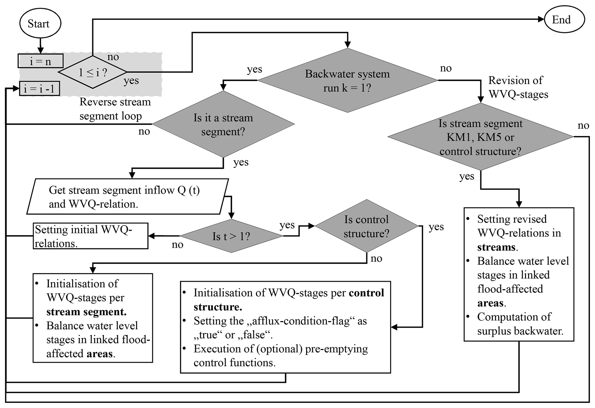
Figure 6 Algorithm to initialise WVQ relations in streams, control structures and areas per backwater system. Details are illustrated in Fig. 5 in the algorithm (a).

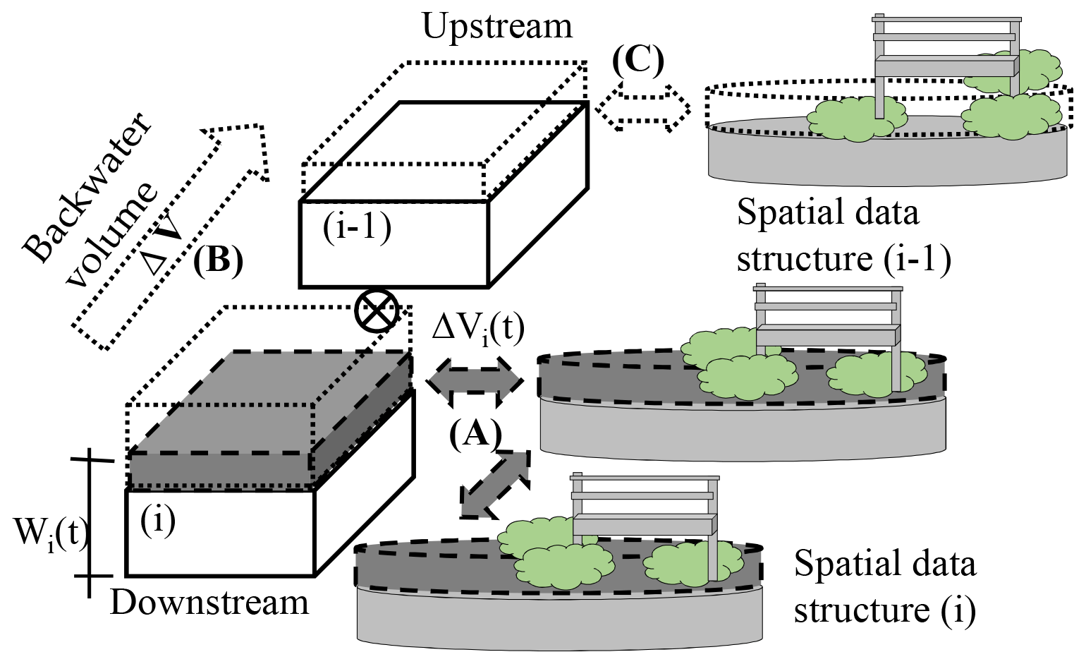
Figure 7 Scheme of the sub-calculation routines (A), (B) and (C) to compute backwater effects in stream segments and adjacent lowland areas (spatial data structures). The sub-calculation routines are part of the main calculation routine (b and c, Fig. 5).

Figure 8 Computation of the upstream-directed backwater effect over stream segments and adjacent lowland areas (e.g. retention areas). Details are illustrated in Fig. 5 in the algorithm (b).

5 Implementation of the hydrological method for calculating backwater effects in Kalypso-NA (4.0)

Implementing the developed method into target software is done for evaluation and application purposes. The implementation is realised in the open-source model Kalypso-NA (4.0), which has constantly been under development and applied for more than 20 years in research and practice. The numerical model features are semi-distributed, deterministic, multi-layered and combined conceptually–physically based. The model shows strengths in short computation times, which is in the range of max 3 min on typical desktop computers (with e.g. i7-5600U CPU processor) for large catchments (ca. 200 km²) using a time step size of 15 min for a 14 d simulation. It is applicable for real-time operational simulations in flood forecasting. In combination with the Kalypso Project providing a user interface, the model Kalypso-NA is applicable for calculating the rainfall–runoff regime in catchments by users who are not familiar with input scripts. Open access for developments and user application is supported by an online-accessible commitment management via the Source Forge platform and a wiki as an online manual. More information about the software product Kalypso and the model Kalypso-NA is provided in the Supplement Sect. S1. Such an open-source module provides accessibility to the implemented methods and therewith supports re-use in other hydrological models. The purpose is to support good scientific practice towards open and reproducible science.

The algorithms in the source code of Kalypso-NA are extended for the integration of the developed methods for backwater effect computation in rivers and adjacent lowland areas. The hydrological numerical model comprises algorithms in the form of time loops executed within a spatial tree structure (time-before-space algorithm) and spatial calculation routines executed within a time loop (space-before-time algorithm). Both approaches are integrated in the source code of Kalypso-NA (4.0) as illustrated in Fig. 9. A time loop nested in a spatial loop accomplishes the simulation of data structures (such as sub-catchments, stream segments, junction nodes or retention areas) in the downstream direction on the basis of the overall results of the upstream data structures. This means that the data structures are computed for the whole simulation period consecutively in the order given by the hydrological network from upstream to downstream. More information about the hydrological network is given in the Supplement Sect. S3. The first implementation (Part A) provides actual time-dependent results of data structures to set control functions or drainage criteria in the hydrological network. This method is applied in the extended algorithm to model processes in sub-catchments like the soil water balance and the downstream-directed flood routing. This algorithm is explained in more detail in Hellmers and Fröhle (2017).

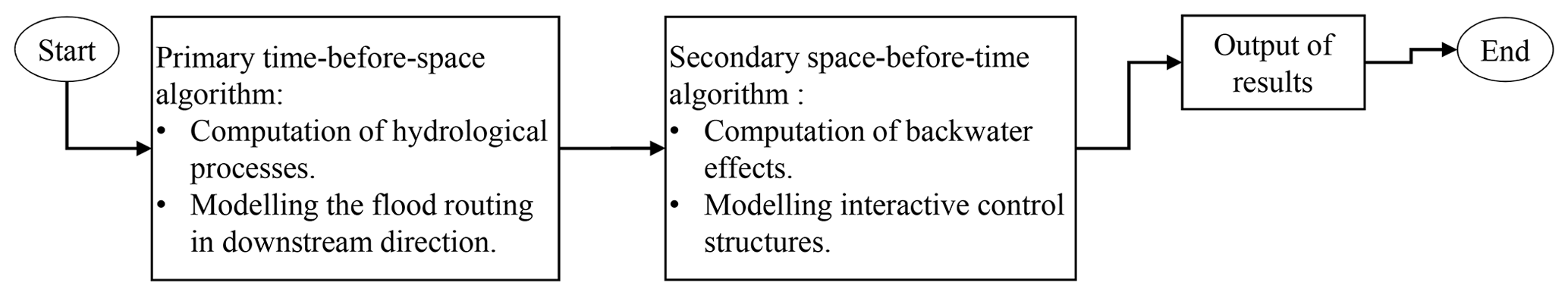
Figure 9 Structure of the implemented primary and secondary algorithm in the source code of Kalypso-NA (4.0). The enhancement of the primary algorithm is published in Hellmers and Fröhle (2017). The new (secondary) algorithm is explained in Sect. 4.3.

Additionally, an algorithm is implemented when spatial calculation routines are nested in time loops. This secondary algorithm provides the overall results of a backwater-affected system per time step before calculating the next time step. The time loop is additionally nested in a backwater system loop. In that calculation routine the backwater effects in streams and adjacent lowland areas as well as the evaporation from submerged water surfaces are computed. This implementation is labelled as space-before-time algorithm and is illustrated in Fig. 5. The implemented hydrological model approach is applicable to other catchment studies, while using physically based input parameters. The input and output parameters are listed in the Supplement Sects. S2 and S5.

6 Exemplary model application and evaluation

The objective of the model evaluation is to determine the reliability of the numerical model results to be in a sufficient range of accuracy for the designated field of application (Law, 2008; Oberkampf and Roy, 2010; Refsgaard and Henriksen, 2004; Sargent, 2014). An evaluation of the extended model Kalypso-NA (4.0) is performed by comparing the results of the numerical model with observed data from gauging stations in the mesoscale catchment Dove–Elbe. This exemplary catchment comprises a tide gate and several sluices, weirs and low-lying catchments drained by pumping stations. The drainage through the tide gate depends on low tide conditions. At high tide, the gate is closed, causing backwater effects in the streams.

6.1 Description of the backwater-affected lowland catchment Dove–Elbe

The mesoscale catchment area Vier- und Marschlande has a size of 175 km² and is located in the south-east of Hamburg, Germany (see Fig. 10). The downstream river segment Dove–Elbe is a stream of 18 km in length and a tributary of the tidally influenced Elbe River. Further tributary streams which drain into this main river segment are the Gose Elbe, Schleusengraben, Brookwetterung and a downstream segment of the Bille. These streams are part of the analysed mesoscale catchment. The soil is mainly peat and clay with a varying spatial distribution and thickness. Another regional-scale catchment (namely of the river Bille) with a size of about 337 km² drains into the study area Vier- und Marschlande. Thus, an overall catchment area of about 512 km² is drained through the tide gate Tatenberger Deichsiel.

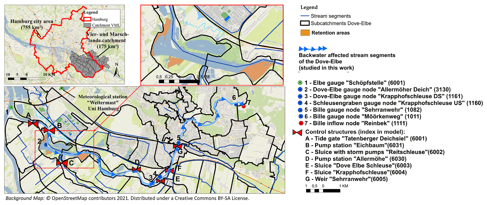
Figure 10 Map of the application study area Vier- und Marschlande (175 km²): sub-catchments, gauging stations (1 to 7), studied backwater-affected streams of the Dove–Elbe, three retention areas in the main stream and control structures (A to G).

The downstream-situated water level in front of the tide gate is affected by a mean tidal range of about 3.7 m (Nehlsen, 2017). The mean low water (MLW) is at about −1.5 m a.s.l., and the mean high water (MHW) is at about 2.2 m a.s.l. The tide gate closes when a water level of about 0.9 m a.s.l. is exceeded in the Elbe River. During the closure period of the tide gate, water is retained in the stream segments of the Vier- und Marschlande catchment, leading to an afflux of water, which causes backwater effects. The numerical model includes 75 sub-catchments, 75 junction nodes, 75 mesoscale stream segments, 7 gauging stations and 7 control structures. These control structures comprise gates, weirs, pumping stations and a tide gate (see Fig. 10). The control functions comprise the opening and closure of gates and sluices or starting of pumps according to defined criteria. The backwater-affected river segments in the Dove–Elbe with a length of about 12.5 km are characterised by wide profiles (width >100 m) and wide flood-prone areas (width >200 m) on the mesoscale.

For the computation of the flood routing, the Kalinin–Miljukov method for mainly irregular profiles with five reservoir parameterisations is applied. An explanation is given in the Supplement Sect. S4.3. Additionally, a scenario simulation is performed within the research project StucK (Long-term drainage management of tide-influenced coastal urban areas with consideration of climate change; https://www.stuck-hh.de, last access: 1 May 2021) with three retention areas (300 000 m²), which are indicated in Fig. 10. The application and evaluation results of the research project StucK for the Dove–Elbe streams as part of the Vier- und Marschlande catchment are summarised in the following section.

6.2 Application and evaluation results

An evaluation of the developed method to compute backwater effects with Kalypso-NA (4.0) is done by comparing numerical model results with data from gauge measurements along the river stream segments of the Dove–Elbe. The analysis of two flood events is presented. Measurements of five gauging stations in the Dove–Elbe stream segments are available for a flood event in February 2011, and the measurements of the downstream gauging station are available for a flood event in February 2002. The locations of gauging stations and control structures are indicated in Fig. 10.

The results at the downstream gauging station (Allermöher Deich) are illustrated in Fig. 11 for the opening and closing function of the tide gate (in red) according to water levels at the downstream gauging station Schöpfstelle in the Elbe River (in dotted violet) for the event in 2002. The tide gate closes when a water level of 0.9 m a.s.l. is exceeded at the downstream gauging station Schöpfstelle. In the illustrated example of February 2002, the tide gate remained closed two times during storm tides, meaning that the Elbe River water level during low tide periods did not fall below the required minimal water level of 0.9 m a.s.l. The long closure times generated a large afflux up to a water level of 1.7 m a.s.l. and consequently large backwater effects in the Dove–Elbe streams. The simulated and observed peak water levels show an average difference of about 0.02 m. The differences in peak water levels are in the range of 0.01 to 0.10 m. This corresponds to a variation of 1 % to 10 % in the streams with a backwater-affected water level variation larger than 1 m. The root mean square error (RMSE) (<0.12 m) and coefficient of determination (R²) (>0.9) of the flood event analysis confirm the good result evaluation. The RMSE and R² show a very good fit for the rising limb of the flood event. Because of an exceptional manual pre-opening of the tide gate by the authority, ca. 1.5 h before reaching the water level of 0.9 m a.s.l. in the Elbe, the simulated control function and observed status of the control structure are not comparable for the falling limb (details are illustrated in Supplement Sect. S6). During the rainfall storm event in February 2011, the water level increased due to backwater effects caused by high flood discharge from upstream catchments. Here, a difference of less than 0.01 m is shown between observed and simulated peak water levels. The scatter plot, the R² and the RMSE for the flood event analysis on 7 to 8 February 2011 show a good concordance. An interactive backwater system is present for the downstream Dove–Elbe river section, which is influenced by the control structures Reitschleuse (blue, Fig. 11) and Dove–Elbe Schleuse (green, Fig. 11). Both control structures depend on thresholds of the downstream water levels in the Dove–Elbe stream segments (black, Fig. 11). In this case, the method to model interactive control systems is applied. The evaluation results show a good performance of the model: the closing and opening times of the sluices according to the thresholds are met.

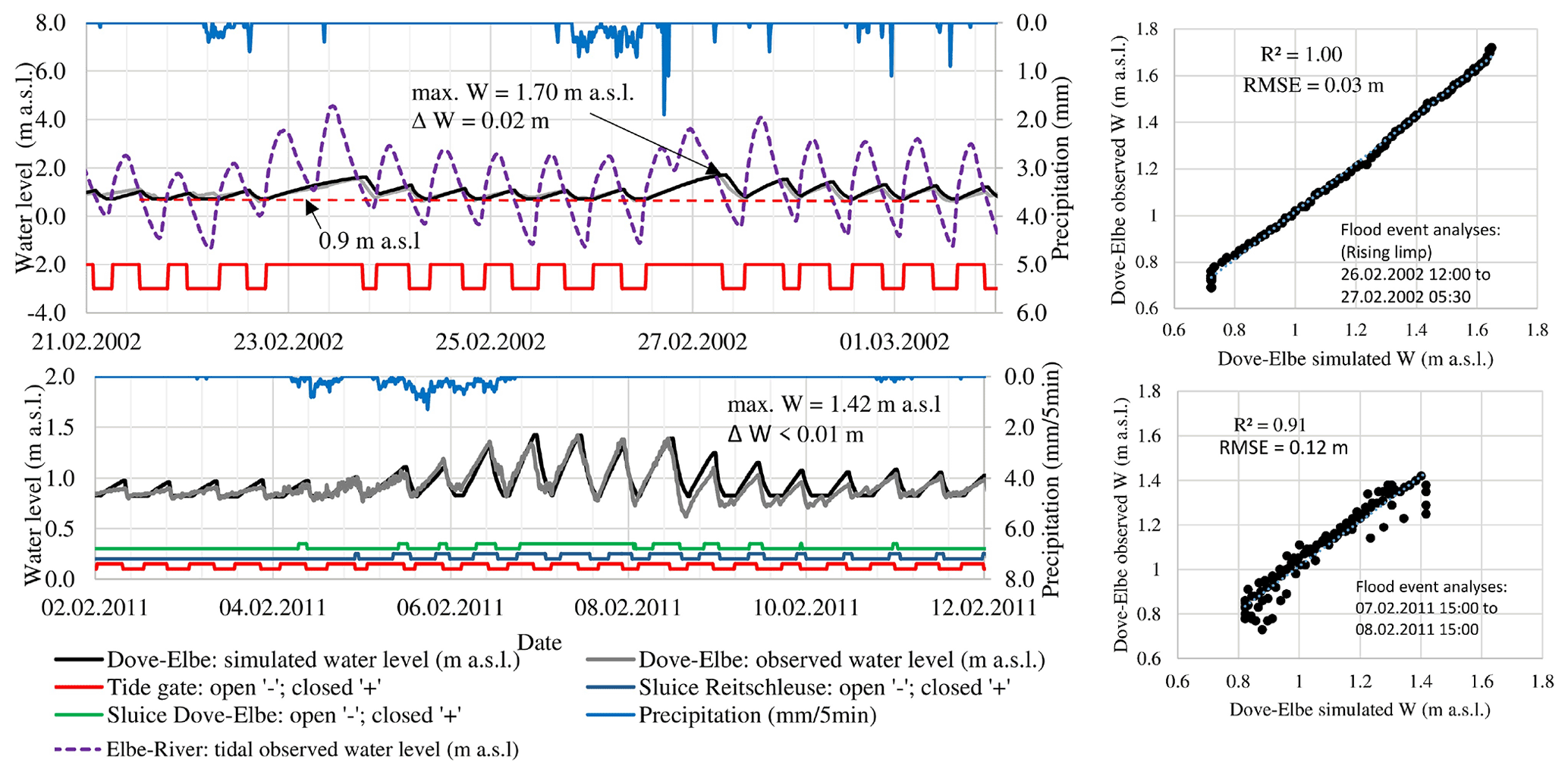
Figure 11 Closure and opening state of the control structures as well as simulated and observed water levels at the downstream gauge Allermöher Deich for the event in February 2002 and February 2011. The tide gate remained closed two times during the storm events in February 2002, meaning that the Elbe River water level during low tide period did not fall below the required minimal water level of 0.9 m a.s.l. The simulated and observed water levels depict a difference of 0.02 to 0.01 m in a stream with a water table fluctuation of about 1 m. The RMSE for the flood event analysis shows a deviation of up to 0.12 m.

Details and further results of the events in February 2002 and February 2011 for the control structures (Tatenberger Schleuse, Reitschleuse and Dove–Elbe Schleuse) are given in the Supplement Sect. S6. The average difference in observed and simulated water level peaks is about ΔW=0.04 m. This corresponds to a difference of about 5 % in relation to the 1 m large fluctuation range of the water table in the stream segments of the Dove–Elbe catchment. In additional to the good fit in peak values, the hydrographs in the Supplement of this article show that the temporal sequence (1) of opening and closing the control systems and (2) of the rising and falling limb in the hydrographs in the river segments is well simulated. The results show a good reliability of the computed flood-routing and backwater effects in streams. It is stated that with these findings the reliability of the numerical model results is in a sufficient range of accuracy for the designated field of application.

In additional to the presented evaluation studies, a flood peak reduction measure is analysed in the research project StucK. By excavating three retention areas with a total size of 330 000 m² from +2 to +1 m a.s.l., an additional retention volume of 330 000 m³ is created when the water level exceeds the riverbanks at +1 m a.s.l. The location of retention areas is indicated in Fig. 10. With the additional retention volume, the peak water level can be reduced by 0.08 m. For the event in 2011 the result is shown in the Supplement Sect. S6. More results of the model application for the research project StucK are published in Fröhle and Hellmers (2020).

7 Discussion of model results and limitations

In this section, achieved objectives, limitations and evaluation results of the developed conceptual method are presented. The method facilitates modelling backwater effects in lowlands caused by flow control structures using a stand-alone hydrological model.

The first reached objective is the possibility to model the effects of tidal ranges on the setting of flow control structures and the resulting backwater effects on the flow regime in lowland streams. This objective is reached using a conceptual hydrological method. The developed, implemented and evaluated method transfers discharges into water levels, which means that backwater volume routing is calculated by taking into account the water level slope along streams and adjacent lowland areas. It applies a pre-defined water level tolerance to calculate the backwater volume routing. The use of physically based input parameters (e.g. profile geometries) extends the application of this hydrological model to other catchment studies. The input parameters comprise, for example, data on the stream profiles, gradients and roughness along the flow path (river streams).

A second reached objective is the parsimony of the numerical model. In comparison to coupled hydrodynamic models, the input parameters are parsimonious, meaning less complex and easier to derive. A third reached objective of the developed method is the direct computation of hydrological processes in backwater-affected areas and streams. For example, the infiltration, groundwater recharge and evaporation of water from submerged areas are simulated. To simulate prospective changes in urbanisation or effects by climate change on precipitation, patterns can be directly defined in the hydrological numerical model. The implementation of the method is realised in the open-source rainfall–runoff model Kalypso-NA (version 4.0). The conceptual method is re-useable to extend other hydrological models which are based e.g. on the often-applied flood-routing methods of Kalinin–Miljukov and Muskingum–Cunge.

There are limitations of the conceptual method in the modelling of spatial and temporal details like the variability in the velocity fields and (tidal) flow regime. In the conceptual method, each stream section is computed as a “reservoir” according to the linear reservoir theory, meaning that the backwater profile is assumed to be flat within each river section. The exactness of the water level heights depends on the defined water level tolerance and the scale of the stream segments in the model. This means, in contrast to hydrodynamic–numerical approaches, that the developed hydrological model does not compute velocity fields within streams and water levels but represents average values per stream segment. This hydrological flood-routing method enables modelling regional-scale backwater-affected catchments (>100 km²) with the requirement to keep the computing times small and with a parsimonious parameterisation. The presented method does not mean to replace coupled hydrodynamic–numerical models to answer specific research questions, e.g. for which two- or three-dimensional velocity fields and a spatial distribution of water levels within river streams or on submerged areas need to be computed.

The evaluation results in Sect. 6 show the applicability of the model for simulating rainfall–runoff regimes and backwater effects in an exemplary lowland catchment (175 km², Hamburg, Germany). This catchment is characterised by a complex flow control system, wherein the drainage is influenced by a tidal range of about 4 m. The flood event analyses confirm good evaluation results: the comparison of observed with simulated results shows a low RMSE (<0.12 m) and a high R² (>0.90). For these application studies, a standard desktop computer with an i7-5600U CPU processor and 2.6 GHz is applied. The computation time is in the range of a maximum of 3 min even for large catchments (here: 175 km²) using a time step size of 15 min for a 14 d simulation period. With these short computation times, the presented method shows good potential to be used in flood forecast simulation models for which results in the form of time series (e.g. water levels and discharges) per river section and flood-prone area are sufficient.

8 Summary and outlook

Numerical models are required in forecast simulations and to assess the consequences of future impacts like changes in magnitude and probability of storm-water events, changes in urbanisation, and changes in predicted mean sea level rise on the runoff regime in catchments. Especially in coastal lowlands, the pressure on storm-water drainage and flow control systems is rising due to a combination of all three impacts. The literature review shows weaknesses in modelling water depths and backwater effects in streams and lowland areas using stand-alone hydrological numerical models. A method to resolve these weaknesses is presented in this article. The developed numerical method is:

1. applicable to model complex drainage and flow control systems in backwater-affected lowlands,

2. efficient by using short runtimes for real-time operational model application,

3. open for further model developments,

4. re-useable for other hydrological model solutions and

5. parsimonious with respect to the complexity of input parameters.

The evaluation results in the application study of the complex and tidally influenced lowland catchment Vier- und Marschlande illustrate good conformance in the simulated backwater effects on the flow regime. In addition to the findings in this article, the published outcomes in Hellmers (2020) and Fröhle and Hellmers (2020) show that the reliability of the numerical model results is in a sufficient range of accuracy for the designated field of application to answer a wide range of hydrological and water management questions. The numerical model is suitable for operational flood forecasting, real-time control, risk analyses, scenario analyses and time series gap filling in micro-scale to regional-scale catchments. The presented method is re-useable for other hydrological numerical models which apply conceptual hydrological flood-routing approaches (e.g. Muskingum–Cunge or Kalinin–Miljukov).