HydroPy (v1.0): a new global hydrology model written in Python

Global hydrological models (GHMs) are a useful tool in the assessment of the land surface water balance. They are used to further the understanding of interactions between water balance components and their past evolution as well as potential future development under various scenarios. While GHMs have been part of the hydrologist's toolbox for several decades, the models are continuously being developed. In our study, we present the HydroPy model, a revised version of an established GHM, the Max Planck Institute for Meteorology's Hydrology Model (MPI-HM). Being rewritten in Python, the new model requires much less effort in maintenance, and due to its flexible infrastructure, new processes can be easily implemented. Besides providing a thorough documentation of the processes currently implemented in HydroPy, we demonstrate the skill of the model in simulating the land surface water balance. We find that evapotranspiration is reproduced realistically for the majority of the land surface but is underestimated in the tropics. The simulated river discharge correlates well with observations. Biases are evident for the annual accumulated discharge; however, they can – at least to some extent – be attributed to discrepancies between the meteorological model forcing data and the observations. Finally, we show that HydroPy performs very similarly to MPI-HM and thus conclude the successful transition from MPI-HM to HydroPy.

1 Introduction

Hydrological models are used in a large number of research and operational applications. These range from the catchment scale, e.g. highly calibrated models simulating discharge for one specific river, towards large temporal and spatial scales, e.g. the global analysis of hydrological extremes in long-term climate projections (e.g. Do et al., 2020). Models employed in the latter type of studies belong to the group of global hydrology models (GHMs) which focus on simulating different components of the hydrological cycle for the whole land surface.

Hydrological modelling looks back at several decades of model development (Bierkens, 2015). Starting from early land surface schemes featuring a single bucket-style soil layer (Manabe, 1969), they grew in complexity over time by implementing plant processes and multi-layer soil hydrology as well as considering human impacts (e.g. Alcamo et al., 1997). Depending on their area of operation, the models differ not only in terms of processes, but also in their technical infrastructure and programming language used. They can be designed for stand-alone applications using meteorological forcing data or be an interactively coupled component in Earth system models. Models with a long legacy are often written in Fortran (e.g. SWAT; Arnold et al., 1998) or C (e.g. VIC; Liang et al., 1994), but other programming languages like Python (e.g. PCR-GLOBWB; Sutanudjaja et al., 2018) are also used. While models have come a long way since their initial concepts, there is still ample opportunity for improvement and extension of their functions. Bierkens (2015) identified issues due to missing geospatial data, calibration and input data quality, but also recognized the need to increase model resolution and eventually include sociological and economical interactions.

In order to face such challenges with our model, the Max Planck Institute for Meteorology's Hydrology Model (MPI-HM; Hagemann and Dümenil, 1997; Stacke and Hagemann, 2012; Telteu et al., 2021), a thorough revision of its source code is required. The MPI-HM is a well-established GHM, which was applied in several intercomparison projects and case studies over the last years (e.g. Haddeland et al., 2011; Wada et al., 2013; Schewe et al., 2013; Prudhomme et al., 2013; Mbaye et al., 2015; Zhao et al., 2017; Rasche et al., 2018; Hagemann et al., 2020; Pokhrel et al., 2021). Nonetheless, after a decade of demand-driven development, the MPI-HM became increasingly difficult to maintain. Furthermore, its source code – originally written in Fortran 77 style and later upgraded with Fortran 90 statements – made debugging and the implementation of new processes unnecessarily cumbersome. Therefore, it was decided to rewrite the model from scratch using Python, thus taking advantage of the high-level routines provided by NumPy (Harris et al., 2020) and xarray (Hoyer and Hamman, 2017).

This revised version of MPI-HM – now renamed HydroPy – uses the same hydrological process formulations and boundary data but is easier to set up and more flexible in terms of spatial resolution, and it offers much higher potential for future enhancement. Consequently, a number of new processes were already implemented. The purpose of this article is to document the setup and structure of HydroPy, including both the revised and newly implemented processes. Furthermore, HydroPy's ability to represent observed hydrological quantities is evaluated. Lastly, an overview of ongoing model development is presented and the challenges encountered during this project are discussed.

2 Model description

HydroPy (Stacke and Hagemann, 2021b) consists of a simplified land surface scheme and a lateral river-routing module. It computes only water fluxes and does not feature an explicit energy balance. Instead, near-surface air temperature is used as input for empirical formulations in energy-related processes, e.g. snowmelt or evaporation. If not mentioned otherwise, the near-surface air temperature (or 2 m temperature) is referred to as surface temperature throughout this study. Spatial resolution, time step, domain size and simulation period are determined from the auxiliary data and meteorological forcing. The default setup, for which simulation data are presented in Sect. 4, uses a spatial resolution of 0.5^∘ and a time step of 1 d.

Data describing land surface conditions and meteorological forcing are expected in SI units, e.g. kg m⁻² for all water storages and kg m⁻² s⁻¹ for water fluxes. Internally, all fluxes are multiplied with the model time step Δt.

Each simulation starts with the computation of several secondary boundary fields derived from the primary input data (details in Sect. 3). As this is done only once per simulation, the numerical costs are low, but compared to the former MPI-HM the number of variables in the land surface data file is reduced from 29 to 18. Thus, new HydroPy users need to spend less effort for compiling the required input data prior to model application. Next, the model loops over the time axis provided by the meteorological forcing data. In the beginning of the loop, surface temperature (T_srf), precipitation (P) and potential evapotranspiration (PET) are read, and the latter two are converted into mass flux per time step. Next, all land cover type (LCT) fractions are updated based on the actual date. This is followed by computing water fluxes for the various processes and updating the respective water storages. Figure 1 displays an overview of the water storages included in HydroPy and their connecting water flows. For most storages, outgoing water fluxes are computed based on the storage state at the start of the actual time step followed by updating the storage state using the actual fluxes. The order of storage updates is snow → skin and canopy → soil → surface water and groundwater → river flow. The related processes are presented in detail in the paragraphs in Sect. 2.2. At the end of every time step, all requested output variables are either written to a file (for time step output) or added to a temporary field for time-averaged output. Thus, no time series of variables need to be kept in memory, which strongly reduces the model's computational demands. All output variables are combined in one NetCDF file per output time step resolution (daily, monthly or yearly). Similar to the input, they are stored in SI units: kg m⁻² for water storages, kg m⁻² s⁻¹ for water fluxes, and m³ and m³ s⁻¹ for the special cases of river storage and river discharge, respectively.

Figure 1 Schematic of the major water storages and fluxes in HydroPy together with the symbols used in the process description (see Sect. 2.2). Most processes only affect each grid cell individually (central column), but river routing also interacts with neighbouring cells (represented by small storage columns). The upper left corner shows the official logo designed for the HydroPy model.

At the end of the time loop, screen output is created, which provides information about the overall water balance and any residuum in the sum of water sources, sinks and storage changes. In the case that the water balance residuum exceeds a given threshold, an additional NetCDF output file is generated, which provides fields containing the water balance components. This acts as an early warning system during model development while implementing new processes. The water balance residuum is diagnosed for every grid cell as a one-dimensional water column and as water volume accumulated over the whole field. Through the latter water balance errors caused by changes in LCT fractions can also be spotted easily.

In the case of errors, there is an option to output time series for single grid cells in which all variables are included as well as partial water balances for the individual water storages at model time step. This supports the identification of processes responsible for a water balance violation.

2.1 Model design and setup

The rationale behind HydroPy is not so much to generate a highly efficient GHM, but rather a model which can be easily understood by scientists and extended with additional processes. Thus, we decided to separate functions based on their purpose (see Fig. 2). The file parameter_class.py contains default options and parameter settings together with variable definitions. The dataio_class.py file handles all input and output functions required by HydroPy, and the file analysis_class.py includes functions related to spin-up, water balance checks and log data. The file utility_routines.py is a compilation of general routines like interpolation. All physical process representations are compiled in respective files describing their overall topic like hydrology, land cover and streamflow processes. This enables us to use the main routine to manage the simulation time loop and call the specific model processes in a clearly arranged manner. Furthermore, this file separation serves as a template for the implementation of extensions.

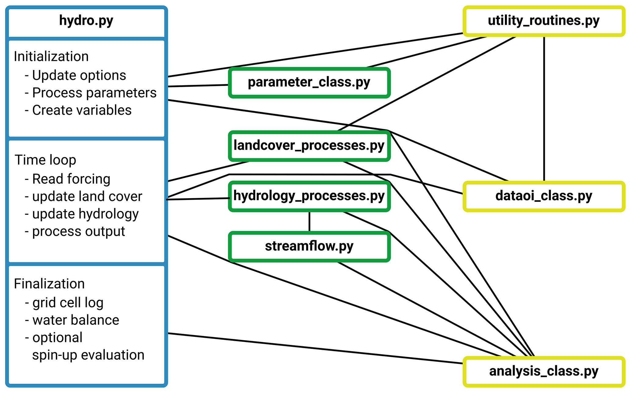
Figure 2 Simplified flowchart of HydroPy depicting the files belonging to the model and their primary interactions. The main routine is shown in blue; process routines are shown in green, and files containing auxiliary functions (I/O, analysis, for example) are shown in yellow.

All variables representing physical properties are organized in a variable class that contains variable attributes and functions. Attributes comprise name, units and grid information. Functions are used to initialize the state of variables, average over time periods and write output as well as restart data. At the start of the model one variable stream is created for all fluxes, states and land cover fractions. This allows for the easy addition of new variables simply by adding some basic information to the respective definition function in the parameter file.

For the majority of hydrological processes, highly optimized NumPy arrays can be used because no information is exchanged between grid cells. However, this is different for river routing. Here, lateral water transport is considered (see Sect. 2.2.5), which requires iterations across the field indices. Such loops are rather slow in an interpreted programming language like Python. For this reason, the river-routing routine was written not only in Python, but also in Fortran. Optionally, the Fortran code can be compiled into a shared library during model runtime using the NumPy tool f2py and called directly from HydroPy. During model development, we made sure that identical results are returned from the Python and Fortran functions. Thus, the Python version can be used during model development and debugging, while the Fortran-based river routing is recommended for production simulations due to its higher efficiency (see Fig. 3).

Figure 3 Sunburst graphs depicting the distribution of model runtime for a global simulation of 1 year at 0.5^∘ resolution without writing any output. Both simulations were conducted on a single node of a high-performance Linux cluster (using an Intel(R) Xeon(R) Platinum 8160 CPU with 2.10 GHz). Values are shown for the pure Python version (left) and the version using Fortran for river routing (right). The visualization was done using Snakeviz (https://jiffyclub.github.io/snakeviz/, last access: 10 December 2020). Note that as HydroPy currently does not utilize parallelization, the runtimes on a standard office laptop are roughly the same.

The model itself can be called via command line and includes a --help option to display calling parameters and further options. A file containing meteorological forcing data is required. Default configurations can be changed by either providing a json-style configuration file or by changing options directly via command line. A detailed technical documentation for model and simulation setup is part of the model repository (Stacke and Hagemann, 2021b).

Although the MPI-HM followed a similar idea in terms of separating processes in different files, the structure of HydroPy is much cleaner and easier to extend and modify due to the use of variable objects. Also, the included diagnostics like spin-up state evaluation and water balance computation as well as the interactive debugging options facilitate the implementation of new processes. And finally, the simulation setup using a simple command line interface and a optional configuration file is a considerable improvement compared to the rather extensive run scripts required for MPI-HM simulations.

2.2 Hydrological processes

The following paragraphs describe all processes implemented in HydroPy in detail, and all variables used are summarized in Table 1. Generally, the processes are identical to the MPI-HM in terms of equations. There are a few exceptions to this rule, which are mentioned below. Furthermore, it should be noted that MPI-HM also includes a simple irrigation scheme, which was used to explore the effect of human impacts on river discharge (e.g. Haddeland et al., 2014). This scheme is not yet implemented in the current version of HydroPy but will become part of a model version dedicated to land management in a future release.

Table 1 Overview of variables used in HydroPy process description, referenced with their equation numbers. Variables directly available for output are denoted by providing their short name in the output column.

2.2.1 Snow processes

In the snow module, the snow storage S_sn is updated based on snowfall P_sn, snowmelt R_sn and liquid snow storage content S_snlq as

$$\begin{array}{}\text{(1)}& \mathrm{\Delta }{S}_{\mathrm{sn}}=P_{\mathrm{sn}}-R_{\mathrm{sn}}+\left\{\begin{array}{ll}{S}_{\mathrm{snlq}},& \text{if }{T}_{\mathrm{srf}}<\mathrm{273.15}\text{ K}\\ \mathrm{0}& \text{otherwise}.\end{array}\right.\end{array}$$

The involved water fluxes are computed as follows. Snowfall – if not provided directly in the forcing data – is diagnosed from precipitation as a function of surface temperature (Eq. 2) following Wigmosta et al. (1994). Snowmelt is calculated using the surface temperature T_srf and day-length fraction f_lday in a degree-day formula based on the HBV model (Bergström, 1992). Naturally, snowmelt is limited by the available snow storage:

$$\begin{array}{ll}{\displaystyle }{P}_{\mathrm{sn}}& {\displaystyle }=P\cdot \text{min}\left\{\mathrm{1},\text{max}\left\{\mathrm{0},{\displaystyle \frac{T_{\mathrm{sn},\max }-T_{\mathrm{srf}}}{T_{\mathrm{sn},\max }-T_{\mathrm{sn},\min }}}\right\}\right\},\\ \text{(2)}& {\displaystyle }& {\displaystyle }\text{with }{T}_{\mathrm{sn},\min }=\mathrm{272.05}\text{ K and }{T}_{\mathrm{sn},\max }=\mathrm{276.45}\text{ K }{\displaystyle }{R}_{\mathrm{sn}}& {\displaystyle }=\text{min}\left\{\left(f_{\mathrm{lday}}\cdot \mathrm{8.3}+\mathrm{0.7}\right)\cdot \left(T_{\mathrm{srf}}-T_{\mathrm{melt}}\right),S_{\mathrm{sn}}+P_{\mathrm{sn}}\right\},\\ \text{(3)}& {\displaystyle }& {\displaystyle }\text{with }{T}_{\mathrm{melt}}=\mathrm{273.15}\text{ K }.\end{array}$$

While MPI-HM used a sine function to estimate the day-length fraction based on the day of the year, this is replaced in HydroPy by explicitly computing the day length based on the Earth's declination (Forsythe et al., 1995). This has the advantage that a reasonable snowmelt is also computed for the Southern Hemisphere. However, the effects are only visible for very few grid cells due to the small extent of snow-affected areas in the Southern Hemisphere.

Part of the snowmelt can be retained (F_snlq) as liquid snow storage content and is either subject to refreezing – if surface temperatures fall below the freezing point – or sustains snowmelt in the next time step. The liquid snow storage content is limited to a maximum of 6 % of the total snow storage, which is a common value also used in other models (e.g. Wigmosta et al., 1994).

$$\begin{array}{}\text{(4)}& {\displaystyle }{F}_{\mathrm{snlq}}& {\displaystyle }=S_{\mathrm{sn}}\cdot f_{\mathrm{snlq},\max }-S_{\mathrm{snlq}},& {\displaystyle }\text{with }& {\displaystyle }{f}_{\mathrm{snlq},\max }=\mathrm{0.06}\text{(5)}& {\displaystyle }{R}_{\mathrm{sn}}& {\displaystyle }=R_{\mathrm{sn}}-F_{\mathrm{snlq}}& {\displaystyle }\text{(6)}& {\displaystyle }{S}_{\mathrm{snlq}}& {\displaystyle }=S_{\mathrm{snlq}}+F_{\mathrm{snlq}}& {\displaystyle }\end{array}$$

2.2.2 Skin and canopy processes

A new addition to HydroPy is the implementation of a skin S_skin and canopy storage S_can, which enhances the evaporation E for the grid cell fractions with the LCTs bare soil f_bare and vegetated f_veg, respectively. Both storages receive input from rainfall P_ra and snowmelt R_sn and provide overflowing water as throughfall towards the ground. Evaporation scales linearly with PET and available water but is additionally limited by the maximum storage content S_prc,max. Mechanistically, storages are treated equally and are described using the index prc to denote the different skin and canopy processes.

$$\begin{array}{}\text{(7)}& \begin{array}{rl}\mathrm{\Delta }{S}_{\mathrm{prc}}& =\left(P_{\mathrm{ra}}+R_{\mathrm{sn}}-E_{\mathrm{prc}}\right)\cdot f_{\mathrm{lct}},\text{ with }\mathrm{prc}=\left\{\text{skin, can}\right\}\\ & \text{ and }\mathrm{lct}=\left\{\text{bare, veg}\right\}\end{array}\end{array}$$

The related fluxes are defined for the respective fraction of the grid cell and scaled to the overall grid cell during the final balancing. Thus, for all storage interactions its content needs to be normalized to the fraction f_lct, resulting in $S_{\mathrm{prc},\mathrm{norm}}=\frac{S_{\mathrm{prc}}}{f_{\mathrm{lct}}}$ so that

$$\begin{array}{}\text{(8)}& {\displaystyle }{f}_{\mathrm{wet}}& {\displaystyle }=\text{min}\left\{\mathrm{1},{\displaystyle \frac{S_{\mathrm{prc},\mathrm{norm}}+P_{\mathrm{ra}}+R_{\mathrm{sn}}}{S_{\mathrm{prc},\max }}}\right\},\text{(9)}& {\displaystyle }{E}_{\mathrm{prc}}& {\displaystyle }=\text{PET}\cdot f_{\mathrm{wet}}\cdot \text{min}\left\{\mathrm{1},{\displaystyle \frac{S_{\mathrm{prc},\mathrm{norm}}+P_{\mathrm{ra}}+R_{\mathrm{sn}}}{f_{\mathrm{wet}}\cdot \text{PET}}}\right\},\text{(10)}& {\displaystyle }{R}_{\mathrm{prc}}& {\displaystyle }=\text{max}\left\{\mathrm{0},S_{\mathrm{prc},\mathrm{norm}}+\left(P_{\mathrm{ra}}+R_{\mathrm{sn}}-E_{\mathrm{prc}}\right)-S_{\mathrm{prc},\max }\right\}.\end{array}$$

While the processes for skin and canopy storage are parameterized similarly, they use specific maximum storage values:

$$\begin{array}{}\text{(11)}& \begin{array}{rl}& \mathrm{\Delta }{S}_{\mathrm{prc},\max }=\\ & {\mathrm{cap}}_{\mathrm{0}}\cdot \left\{\begin{array}{ll}\mathrm{1},& \text{if }\mathrm{prc}=\text{skin}\\ \text{LAI}& \text{if }\mathrm{prc}=\text{can}\end{array}\right.,\text{with }{\mathrm{cap}}_{\mathrm{0}}=\mathrm{0.2}.\end{array}\end{array}$$

Both runoff fluxes are scaled by the respective LCT fractions and combined to provide the throughfall R_tr that reaches the soil surface:

$$\begin{array}{}\text{(12)}& R_{\mathrm{tr}}=R_{\mathrm{skin}}\cdot f_{\mathrm{bare}}+R_{\mathrm{can}}\cdot f_{\mathrm{veg}}.\end{array}$$

2.2.3 Soil processes

HydroPy employs a single-layer soil scheme in which the storage S_so provides water for transpiration E_T, bare soil evaporation E_bs and drainage R_gr (used synonymously for groundwater recharge or subsurface runoff) towards a shallow groundwater storage. Furthermore, its content determines the surface runoff R_srf. The soil storage does not represent the physical soil over a given depth but only the water column stored in the soil. Thus, its maximum value is limited by the maximum soil water capacity S_so,max. The soil moisture storage is defined as

$$\begin{array}{}\text{(13)}& \mathrm{\Delta }{S}_{\mathrm{so}}=R_{\mathrm{tr}}-R_{\mathrm{srf}}-R_{\mathrm{gr}}-E_{\mathrm{T}}\cdot f_{\mathrm{veg}}-E_{\mathrm{bs}}\cdot f_{\mathrm{bare}}.\end{array}$$

Both drainage and surface runoff are implemented identically to these fluxes in MPI-HM using the same parameter values. Drainage, following the formulation by Dümenil and Todini (1992), is defined such that it scales linearly with soil moisture content up to a given threshold. Above, saturated flow is assumed, resulting in accelerated downward percolation with exponential scaling:

$$\begin{array}{ll}\text{(14)}& {\displaystyle }{R}_{\text{gr,low}}& {\displaystyle }=R_{\text{gr,min}}\cdot \mathrm{\Delta }t\cdot {\displaystyle \frac{S_{\mathrm{so}}}{S_{\mathrm{so},\max }}}& {\displaystyle }{\displaystyle }{R}_{\text{gr,high}}& {\displaystyle }=\left(R_{\text{gr,max}}-R_{\text{gr,min}}\right)\cdot \mathrm{\Delta }t\\ {\displaystyle }& {\displaystyle }\cdot {\left({\displaystyle \frac{S_{\mathrm{so}}-S_{\text{so,grmax}}}{S_{\mathrm{so},\max }-S_{\text{so,grmax}}}}\right)}^{R_{\text{gr,exp}}},\\ \text{(15)}& {\displaystyle }& {\displaystyle }\text{ with }{R}_{\text{gr,exp}}=\mathrm{1.5}.\end{array}$$

Both are combined as follows.

$$\begin{array}{}\text{(16)}& \begin{array}{rl}& R_{\mathrm{gr}}=\\ & \left\{\begin{array}{ll}\mathrm{0},& \text{if }{S}_{\mathrm{so}}\le S_{\text{so,grmin}}\text{ or }{T}_{\mathrm{srf}}<\mathrm{273.15}\text{ K}\\ R_{\text{gr,low}}& \text{if }{S}_{\text{so,grmin}}<S_{\mathrm{so}}\le S_{\text{so,grmax}}\\ R_{\text{gr,low}}+R_{\text{gr,high}}& \text{if }{S}_{\text{so,grmax}}<S_{\mathrm{so}}\end{array}\right.\end{array}\end{array}$$

The soil moisture thresholds S_so,grmin and S_so,grmax are products of S_so,max using the factors 0.05 and 0.9, respectively. The minimum and maximum drainage, R_gr,min and R_gr,max, are set to 2.7e−7 and 2.7e−5 [kg m⁻² s⁻¹]. As both parameters are given as flux per second, they need to be multiplied with the model time step Δt. All drainage-related model parameters are taken from Roeckner et al. (1992).

The surface runoff R_srf representation follows the improved Arno scheme (Hagemann and Gates, 2003). It assumes that S_so,max is not homogeneous for a whole grid cell but varies on the sub-grid scale. Thus, parts of the grid cell in which the local storage capacity is low can already generate surface runoff even though the cell average soil moisture state is still below its average maximum moisture-holding capacity. Therefore, a fraction of R_tr is converted into R_srf as soon as the minimum soil moisture content is exceeded. This is realized by mapping S_so onto the sub-grid soil moisture capacity distribution parameters denoted by the index _sg:

$$\begin{array}{}\text{(17)}& \begin{array}{rl}& S_{\text{so,sg}}=\\ & \left\{\begin{array}{l}{S}_{\text{so,sg,max}}-\left(S_{\text{so,sg,max}}-S_{\text{so,sg,min}}\right)\\ \cdot {\left(\mathrm{1}-\frac{S_{\mathrm{so}}-S_{\text{so,sg,min}}}{S_{\mathrm{so},\max }-S_{\text{so,sg,min}}}\right)}^{\frac{\mathrm{1}}{\mathrm{1}+b}}& \text{if }{S}_{\mathrm{so}}>S_{\text{so,sg,min}}\\ S_{\mathrm{so}}& \text{otherwise},\end{array}\right.\end{array}\end{array}$$

where b is a shape parameter describing the distribution of sub-grid soil moisture capacities within a grid cell (see Sect. 3). Overall R_srf is computed as follows:

$$\begin{array}{}\text{(18)}& {\displaystyle }\begin{array}{rl}& R_{\mathrm{srf}}=\\ & \left\{\begin{array}{ll}{R}_{\mathrm{tr}}& \text{if }{T}_{\mathrm{srf}}<\mathrm{273.15}\text{ K}\\ \mathrm{0}& \text{if }{S}_{\text{so,sg}}+R_{\mathrm{tr}}\le S_{\text{so,sg,min}}\text{ or }{R}_{\mathrm{tr}}=\mathrm{0}\\ R_{\mathrm{tr}}+\text{max}\left\{\mathrm{0},S_{\mathrm{so}}-S_{\mathrm{so},\max }\right\}& \text{if }{S}_{\text{so,sg}}+R_{\mathrm{tr}}>S_{\text{so,sg,max}}\\ R_{\mathrm{tr}}-\text{max}\left\{\mathrm{0},S_{\text{so,sg,min}}-S_{\mathrm{so}}\right\}\\ -\frac{S_{\text{so,sg,max}}-S_{\text{so,sg,min}}}{\mathrm{1}+b}\cdot \left(c_{\mathrm{1}}-c_{\mathrm{2}}\right)& \text{otherwise},\end{array}\right.\end{array}\end{array}$$

where c₁ and c₂ are further scaling operations put into separate equations for convenience.

$$\begin{array}{}\text{(19)}& {\displaystyle }{c}_{\mathrm{1}}& {\displaystyle }=\text{min}\left\{\mathrm{1},{\left({\displaystyle \frac{S_{\text{so,sg,max}}-S_{\text{so,sg}}}{S_{\text{so,sg,max}}-S_{\text{so,sg,min}}}}\right)}^{\mathrm{1}+b}\right\}\text{(20)}& {\displaystyle }{c}_{\mathrm{2}}& {\displaystyle }=\text{max}\left\{\mathrm{0},{\left({\displaystyle \frac{S_{\text{so,sg,max}}-S_{\text{so,sg}}-R_{\mathrm{tr}}}{S_{\text{so,sg,max}}-S_{\text{so,sg,min}}}}\right)}^{\mathrm{1}+b}\right\}\end{array}$$

The sub-grid parameters S_so,sg,max and S_so,sg,min that determine the range of sub-grid maximum water capacity variability are spatially distributed fields, and their generation is discussed in Sect. 3.

As for runoff, transpiration E_T and bare soil evaporation E_bs are implemented based on the respective MPI-HM equations (which themselves are derived from Roeckner et al., 1996; Warrilow et al., 1986; Bauer et al., 1983) and use a linear scaling with soil moisture content. Even though they are attributed to specific LCT fractions, which are the vegetated f_veg and bare soil f_bare parts of the grid cell, they do not rely on fraction-specific soil moisture storages but use the grid cell average for simplicity. Still, it has to be considered that part of the evaporative demand on these fractions is already satisfied due to canopy and skin evaporation.

$$\begin{array}{ll}{\displaystyle }{E}_{\mathrm{T}}& {\displaystyle }=\left(\text{PET}-E_{\mathrm{can}}\right)\\ {\displaystyle }& {\displaystyle }\cdot \text{min}\left\{\mathrm{1},\text{max}\left\{\mathrm{0},{\displaystyle \frac{S_{\mathrm{so}}-S_{\mathrm{so},\mathrm{wilt}}}{f_{\mathrm{so},\mathrm{crit}}\cdot S_{\mathrm{so},\max }-S_{\mathrm{so},\mathrm{wilt}}}}\right\}\right\},\\ \text{(21)}& {\displaystyle }& {\displaystyle }\text{ with }{f}_{\mathrm{so},\mathrm{crit}}=\mathrm{0.75}{\displaystyle }{E}_{\mathrm{bs}}& {\displaystyle }=\left(\text{PET}-E_{\mathrm{skin}}\right)\\ {\displaystyle }& {\displaystyle }\cdot \text{min}\left\{\mathrm{1},\text{max}\left\{\mathrm{0},{\displaystyle \frac{S_{\mathrm{so}}-f_{\text{so,bs,low}}\cdot S_{\mathrm{so},\max }}{\left(\mathrm{1}-f_{\text{so,bs,low}}\right)\cdot S_{\mathrm{so},\max }}}\right\}\right\},\\ \text{(22)}& {\displaystyle }& {\displaystyle }\text{ with }{f}_{\text{so,bs,low}}=\mathrm{0.05}\end{array}$$

Again, the spatially distributed data fields S_so,max and S_so,wilt are part of the input dataset (Sect. 3).

Runoff and evaporation fluxes are visualized in Fig. 4 for a single grid cell. There, the threshold-dependent change in the scaling of individual fluxes with respect to specific thresholds can be easily recognized.

Figure 4 Behaviour of runoff (left panel; surface runoff in red, drainage in green) and evaporation (right panel; transpiration in blue, bare soil evaporation in orange) fluxes calculated as a function of soil moisture for a single grid cell. All variables are normalized using their maximum values for better comparison. Dashed lines indicate variable-specific thresholds, which are defined in Sect. 2.2.3. Note that drainage is visualized using a logarithmic axis.

2.2.4 Surface water and shallow groundwater processes

The implementation of surface water has been modified compared to the formulation used in MPI-HM and described in Stacke and Hagemann (2012). In MPI-HM the vertical land surface water balance module and the river-routing module were strongly separated, each featuring storages restricted to be used within the respective module. The sole exception was the surface water storage resulting from ponding water on the land surface and hence used to represent small creeks, lakes and wetlands. This storage was part of the vertical land surface water balance but could also interact with the lateral river-routing scheme. In HydroPy, we simplify the representation of lakes and wetlands and utilize storages already part of the routing scheme as will be explained in the next paragraphs.

The river-routing scheme used in both MPI-HM and HydroPy is the Hydrological Discharge Model (HD-Model; Hagemann and Dümenil, 1997; Hagemann et al., 2020). To represent river flow, it employs three storages: the overland flow storage receives the local grid cell's surface runoff, the baseflow storage receives the local drainage and the river flow storage receives inflow from upstream grid cells. All three storages provide water to the next downstream grid cell. The purpose of the overland and baseflow storages is to delay the flow of both runoff components before they enter the river. As such, they represent a major function of surface water (e.g. small lakes, wetlands and creeks smaller than the grid cell size) and shallow groundwater – even though no effort was taken to explicitly represent any other hydrological functions.

In HydroPy, the former overland and baseflow storages are used as surface water S_sw and groundwater storages S_gw. However, we would like to emphasize that both storage representations are very limited and are not expected to simulate all relevant lake and groundwater processes. Neither circulation within lakes nor confined aquifers, fossil groundwater or lateral water movement within large-scale aquifers are considered at this point. The surface water balance is adapted to allow for interception of rainfall and snowmelt as well as water loss due to evaporation over the surface fraction f_sw, while the shallow groundwater balance only considers groundwater recharge R_gr and runoff R_gw.

$$\begin{array}{ll}{\displaystyle }\mathrm{\Delta }{S}_{\mathrm{sw}}& {\displaystyle }=\left(P_{\mathrm{ra}}+R_{\mathrm{sn}}-\text{PET}\right)\cdot f_{\mathrm{sw}}+R_{\mathrm{srf}}-R_{\mathrm{sw}},\\ \text{(23)}& {\displaystyle }& {\displaystyle }\text{ where }{f}_{\mathrm{sw}}=\text{max}\left\{f_{\mathrm{lake}},f_{\mathrm{wetland}}\right\}\text{(24)}& {\displaystyle }\mathrm{\Delta }{S}_{\mathrm{gw}}& {\displaystyle }=R_{\mathrm{gr}}-R_{\mathrm{gw}}\end{array}$$

Surface water evaporation is set to PET as long as there is enough water available over the surface water fraction. Surface water and groundwater runoff are both computed as

$$\begin{array}{}\text{(25)}& R_{\mathrm{prc}}=S_{\mathrm{prc}}\cdot {\displaystyle \frac{\mathrm{1}}{{\text{LAG}}_{\mathrm{prc}}+\mathrm{1}}},\text{ with prc}=\left\{\text{sw,gw}\right\}.\end{array}$$

The storage retention time LAG_prc is computed based on the inner grid cell slope and grid cell size. More details can be found in Sect. 3.

2.2.5 River routing

River routing is realized based on formulations from the HD-Model, which was also part of the MPI-HM. It applies a river flow cascade with up to five intermediate storages (c_max), as well as parameterizations for river flow retention times, and uses prescribed routing directions. It is the only part of HydroPy that uses a volumetric unit [m³] instead of water columns. Thus, runoff needs to be converted using the grid cell area A_gc. The river flow storages S_rf,n for the individual cascade members n are defined as follows.

$$\begin{array}{ll}{\displaystyle }\mathrm{\Delta }{S}_{\mathrm{rf},n}& {\displaystyle }=Q_{\mathrm{rf},n-\mathrm{1}}-Q_{\mathrm{rf},n}\\ \text{(26)}& {\displaystyle }& {\displaystyle }\text{ with }n=\left\{\mathrm{1},..,c_{max}\right\}\text{ where }\text{(27)}& {\displaystyle }{Q}_{\mathrm{rf},n}& {\displaystyle }=\left(S_{\mathrm{rf},n}+Q_{\mathrm{rf},n-\mathrm{1}}\right)\cdot {\displaystyle \frac{\mathrm{1}}{{\text{LAG}}_{\mathrm{rf}}+\mathrm{1}}}& {\displaystyle }\text{(28)}& {\displaystyle }{Q}_{\mathrm{rf},\mathrm{0}}& {\displaystyle }=\sum Q_{\mathrm{rf},\mathrm{up}}& {\displaystyle }\text{(29)}& {\displaystyle }{Q}_{\mathrm{rf}}& {\displaystyle }=Q_{\mathrm{rf},c_{max}}+\left(R_{\mathrm{sw}}+R_{\mathrm{gw}}\right)\cdot \mathrm{0.001}\cdot A_{\mathrm{gc}}& {\displaystyle }\end{array}$$

The index “up” denotes the river flow Q_rf from upstream grid cells. High river flow velocities combined with a daily model time step can lead to numerical instabilities at a given resolution in the case that water travels more than one grid cell. For this reason, the river flow cascade as well as the routing are encapsulated in a sub-step time loop which is called several times per model time step.

3 Land surface data

In HydroPy effort was made to reduce the number of land surface datasets to a minimum. Thus, very specialized datasets like the river flow lag times are computed by HydroPy itself instead of requiring the model user to pre-process such data. Of course, this comes with the disadvantage of a slight increase in computational demand, but as these data fields are only computed once per simulation, this is hardly noticeable. All land surface data fields are collected in one parameter file (Stacke and Hagemann, 2021a).

3.1 Primary data fields

All computations in HydroPy are restricted to land cells which are defined in the land–sea mask as values >0. All other fields providing fractional information on LCTs are normalized with the land–sea mask and therefore represent relative fractions. The LCTs considered comprise glaciers, permafrost, lakes, wetlands and vegetation. Glacier cells (Hagemann, 2002) are omitted from the simulation if the glaciers cover the full land surface fraction, while permafrost (GEWEX ISLSCP Project, 2007) strongly reduces the soil's capability to store water. The lake and wetland fractions are based on the Global Lake and Wetland Database (GLWD; Lehner and Döll, 2004). They are utilized to scale surface water evaporation and surface water runoff as well as to modify lateral flow velocities. The lake fractions are used without any modifications, but wetlands were restricted to the classes floodplains and peatlands for this study. Thus, we can best resemble the general wetland distribution used for the predecessor of HydroPy and facilitate a clean comparison between the two (see Sect. 4.4). The vegetated fraction is taken from the Land Surface Parameters Dataset 2 (LSP2; Hagemann, 2002) and included into the HydroPy parameter file as monthly mean climatology. Another vegetation parameter dataset used by HydroPy is the monthly leaf area index (LAI) climatology, which also originates from the LSP2 dataset. For both, the monthly mean values are linearly interpolated to match the respective model time step. The vegetation fraction affects canopy processes and transpiration, while the LAI defines the size of the canopy storage.

Three topographical variables are included in the parameter file, which are all based on the ETOPO1 dataset (Amante and Eakins, 2009). These variables are the grid cell mean surface orography and its standard deviation as well as the average slope within a grid cell. The slope was initially computed at the native dataset resolution (${\mathrm{1}}^{\prime }\approx \mathrm{0}$.01^∘). Mean slope, mean orography and its standard deviation were determined during upscaling from the original to the target resolution of 0.5^∘. Both mean orography and slope are used to derive lateral water flow velocities in surface water, groundwater and rivers. The orographical standard deviation plays a role in determining the surface runoff.

The majority of the remaining parameters are related to soil properties. Maximum soil moisture capacity and plant-available water are computed following the procedure described in Hagemann et al. (1999), but with a different dataset as a source for plant-available water. Values for plant-available water are derived via a multi-linear regression from a dataset of optimized plant rooting depth (Kleidon, 2004) and high-resolution land cover data (Loveland et al., 2000). The same data were also used in the MPI-ESM, the Earth system model of the Max Planck Institute for Meteorology (Hagemann and Stacke, 2015) . While the maximum soil moisture capacity S_so,max affects all soil processes, the plant-available water S_so,wava is needed to calculate transpiration. Further properties are the sub-grid minimum and maximum soil moisture capacity as well as an exponent b_sg that describes the distribution of sub-grid soil moisture capacities within every model grid cell. All three of these values are discussed in Hagemann and Gates (2003) and are needed to compute surface runoff.

The final two parameters describe the river-routing network using routing target indices. There is one field for each geographical dimension, i.e. latitude and longitude, and each grid cell is assigned with a flow target in the respective direction, which must be one of the eight neighbouring grid cells. Note that the target is provided as a grid cell index, not as a geographical coordinate. As the indices follow Python notation, they start at 0. For cells without any valid flow target, their own indices are used. The directions prescribed with the routing target indices for HydroPy are identical to the one used by MPI-HM. After their first publication in Hagemann and Dümenil (1997), they were continuously improved during the last years.

3.2 Derived data fields

Not all land surface variables are used directly in the simulated processes. Instead, they are (also) used to derive other variables. This is done during model initialization and will be discussed in the following.

The impact of permafrost on the simulation is represented purely from a hydrological viewpoint. All soil moisture capacity variables are reduced to reflect the fact that only a small part of the soil column is not frozen and may actively contribute to the water balance. The reduction factor f_pe,red is computed based on the permafrost cover fraction f_pe as

$$\begin{array}{}\text{(30)}& \begin{array}{rl}{f}_{\mathrm{pe},\mathrm{red}}& ={\displaystyle \frac{S_{\mathrm{pe},\max }\cdot f_{\mathrm{pe}}+S_{\mathrm{so},\max }\cdot \left(\mathrm{1}-f_{\mathrm{pe}}\right)}{S_{\mathrm{so},\max }}}\\ & \text{ with }{S}_{\mathrm{pe},\max }=\mathrm{50}{\mathrm{kg}\mathrm{m}}^{-\mathrm{2}}\end{array}\end{array}$$

and then used to scale all soil moisture capacity fields:

$$\begin{array}{}\text{(31)}& S=S\cdot f_{\mathrm{pe},\mathrm{red}}\text{ with }S=\left\{S_{\mathrm{so},\max },S_{\mathrm{so},\mathrm{wilt}},S_{\text{so,sg,min}},S_{\text{so,sg,max}}\right\}.\end{array}$$

Next, the shape parameter b describing the sub-grid distribution of soil moisture capacities (see Eqs. 15, 19 and 20) is derived based on the distribution parameter b_sg and modified with the normalized orographical standard deviation b_oro:

$$\begin{array}{ll}{\displaystyle }{b}_{\mathrm{oro}}& {\displaystyle }={\displaystyle \frac{{\mathit{\sigma }}_h-{\mathit{\sigma }}_{\mathrm{0}}}{{\mathit{\sigma }}_h+{\mathit{\sigma }}_{max}}},\\ \text{(32)}& {\displaystyle }& {\displaystyle }\text{ where }{\mathit{\sigma }}_{\mathrm{0}}=\mathrm{100}\text{m and }{\mathit{\sigma }}_{max}=\mathrm{1000}\text{m},\text{(33)}& {\displaystyle }b& {\displaystyle }=\left\{\begin{array}{ll}{b}_{\mathrm{sg}}+b_{\mathrm{oro}}& \text{if }{b}_{\mathrm{oro}}>\mathrm{0.01}\\ b_{\mathrm{sg}}& \text{otherwise},\end{array}\right.& {\displaystyle }\end{array}$$

where σ_h is the standard deviation of sub-grid orography, while the parameters σ₀ and σ_max need to be modified according to the model's spatial resolution.

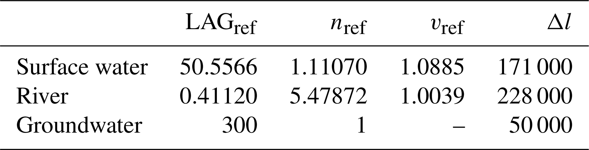
Finally, the retention times (LAG) are determined, which are used in the simulation of surface water and shallow groundwater flow (Eq. 25) as well as river flow (Eq. 27). In all three cases, reference values obtained by sensitivity experiments (Table 3, Hagemann and Dümenil, 1997) for a representative grid cell are modified using the actual properties of grid cells for the remaining part of the land surface – specifically a reference lag time, the flow distance Δl and the flow velocity v. The flow velocity is computed based on the slope s as

$$\begin{array}{}\text{(34)}& v=\text{max}\left\{v_{min},c\cdot s^{\mathit{\alpha }}\right\},\text{ with }c=\mathrm{2}\text{, }\mathit{\alpha }=\mathrm{0.1},\end{array}$$

with the minimum flow velocity set to 0.1 [m s⁻¹]. The actual lag for surface water sw and river flow rf is obtained by modifying the reference lag time (see Table 3) for these processes prc.

$$\begin{array}{}\text{(35)}& \begin{array}{rl}{\mathrm{LAG}}_{\mathrm{prc}}& ={\mathrm{LAG}}_{\mathrm{prc},\mathrm{ref}}\cdot {\displaystyle \frac{\mathrm{\Delta }{l}_{\mathrm{prc}}}{\mathrm{\Delta }{l}_{\mathrm{prc},\mathrm{ref}}}}\cdot {\displaystyle \frac{v_{\mathrm{prc},\mathrm{ref}}}{v}},\\ & \text{ with }\mathrm{prc}=\left\{\mathrm{sw},\mathrm{rf}\right\}\end{array}\end{array}$$

As surface water flow is limited to the respective grid cells, the flow distance Δl_sw is set to the cell's diameter and the slope to the average slope within the grid cell. In contrast, river flow transports water from one cell to the next. Thus, the flow distance Δl_rf is measured as the distance between the centres of a grid cell and its downstream grid cell. Similarly, the slope is computed based on the height difference Δh between the current and downstream grid cell as $s=\frac{\mathrm{\Delta }h}{\mathrm{\Delta }{l}_{\mathrm{rf}}}$. Compared to surface water and river flow, shallow groundwater flow is assumed to be more independent of surface slope, and the reference lag is modified using the grid cell diameter as flow distance and the normalized variation in orography b_oro.

$$\begin{array}{}\text{(36)}& {\mathrm{LAG}}_{\mathrm{gw}}={\mathrm{LAG}}_{\mathrm{gw},\mathrm{ref}}\cdot {\displaystyle \frac{\mathrm{\Delta }{l}_{\mathrm{gw}}}{\mathrm{\Delta }{l}_{\mathrm{gw},\mathrm{ref}}}}\cdot {\displaystyle \frac{\mathrm{1}}{\mathrm{1}-b_{\mathrm{oro}}+\mathrm{0.01}}}\end{array}$$

Additionally, the maximum number of cascade storages c_max (see Eq. 26) is assigned to surface water and river properties. The reference values are listed in Table 3. The lag times of surface water and river flow are further modified if the lake or wetland fractions are large enough to interact with lateral water flow as described in Hagemann and Dümenil (1998). Here, it is assumed that a small water fraction hardly impacts lateral flow velocities but slows down flow velocity significantly if a certain threshold $f_{\mathrm{lct},\mathrm{crit}}=\mathrm{0.5}$ is crossed. This behaviour is reflected in the following equations, with which the flow reduction f_lct,red is computed.

$$\begin{array}{}\text{(37)}& \begin{array}{rl}{f}_{\mathrm{lct},\mathrm{red}}& =\mathrm{0.5}\cdot \left(\tanh \left(\mathrm{4}\cdot \mathit{\pi }\cdot \left(f_{\mathrm{lct}}-f_{\mathrm{lct},\mathrm{crit}}\right)\right)+\mathrm{1}\right)\\ & \text{ where }\mathrm{lct}=\left\{\text{lake, wetland}\right\}\end{array}\end{array}$$

The flow velocity of both processes prc is normalized with reference flow velocities v_lct,ref for the land cover types (LCTs) lakes and wetlands – set to 0.01 and 0.06 m s⁻¹, respectively – and scaled with the flow reduction.

$$\begin{array}{}\text{(38)}& {\displaystyle }{v}_{\mathrm{prc}}& {\displaystyle }={\displaystyle \frac{\mathrm{\Delta }{l}_{\mathrm{prc}}}{{\text{LAG}}_{\mathrm{prc}}\cdot c_{\max ,\mathrm{prc}}\cdot \mathrm{\Delta }t}}\text{, with }\mathrm{prc}=\left\{\mathrm{sw},\mathrm{rf}\right\}\text{(39)}& {\displaystyle }{v}_{\mathrm{prc},\mathrm{red}}& {\displaystyle }=v_{\mathrm{prc}}\cdot \left(\mathrm{1}-\left(\mathrm{1}-{\displaystyle \frac{v_{\mathrm{prc}}}{v_{\mathrm{lct},\mathrm{ref}}}}\cdot f_{\mathrm{lct},\mathrm{red}}\right)\right)\end{array}$$

The number of storages within the flow cascade and the lag time are then updated accordingly.

$$\begin{array}{}\text{(40)}& {\displaystyle }{c}_{\max ,\mathrm{prc}}& {\displaystyle }=\left(c_{\max ,\mathrm{prc}}-\mathrm{1}\right)\cdot \left(\mathrm{1}-f_{\mathrm{lct},\mathrm{red}}\right)+\mathrm{1}\text{(41)}& {\displaystyle }{\text{LAG}}_{\mathrm{prc}}& {\displaystyle }={\displaystyle \frac{\mathrm{\Delta }{l}_{\mathrm{prc}}}{v_{\mathrm{prc},\mathrm{red}}\cdot c_{\max ,\mathrm{prc}}\cdot \mathrm{\Delta }t}}\end{array}$$

These computations are done for both water storage types prc ={surface water, river} and both land cover types lct ={lake, wetland}. As a final step, all retention times are scaled such that the maximum cascade storage number c_max becomes an integer value and can easily be applied in an iteration.

Hagemann (2002)Hagemann (2002)GEWEX ISLSCP Project (2007)Lehner and Döll (2004)Lehner and Döll (2004)Hagemann (2002)Hagemann (2002)Amante and Eakins (2009)Amante and Eakins (2009)Amante and Eakins (2009)Hagemann and Stacke (2015)Hagemann and Stacke (2015)Hagemann and Gates (2003)Hagemann and Gates (2003)Hagemann and Gates (2003)Hagemann and Dümenil (1997)Hagemann and Dümenil (1997)

Table 2 Land surface data variables and their use (directly or as input for derived variables) in the default setup of HydroPy. A symbol is provided for all variables that are used in equations in the hydrological process (Sect. 2.2) or input data description (Sect. 3).

Table 3 Reference values for lateral water flow computation obtained from sensitivity simulations described in Hagemann and Dümenil (1997).

4 Evaluation

The HydroPy evaluation is based on a global simulation, set up at 0.5^∘ spatial resolution with a time step of 1 d. Precipitation and surface temperature time series were taken directly from the Global Soil Wetness Project Phase 3 forcing data (GSWP3, Dirmeyer et al., 2006), while potential evaporation was computed from the same dataset in a pre-processing step using the Penman–Monteith reference evaporation approach (Allen et al., 1998). The simulation period was initialized with a spin-up run over 50 iterations of the year 1979 and then run until 2014. The last 30 years were used for the evaluation and comparison against different observational datasets.

4.1 Simulation spin-up

While it is possible to convert restart files from MPI-HM to initialize HydroPy, the much cleaner way is to start with empty storages and run the model until the trends in its storages become reasonably small. With the currently implemented processes, a time period of 50 years was considered to be sufficient for this task.

The upper left map in Fig. 5 shows the total water storage (TWS) trends during the first 10 years of the spin-up simulation with values up to 100 $\mathrm{kg}{\mathrm{m}}^{-\mathrm{2}}{\mathrm{a}}^{-\mathrm{1}}$. The largest trends are found within the tropical zone and in the south-eastern monsoon region due to the large amount of precipitation together with relatively deep soils that provide a large potential storage. The TWS trends for the last 10 years of spin-up (Fig. 5, upper right map) are below 1 $\mathrm{kg}{\mathrm{m}}^{-\mathrm{2}}{\mathrm{a}}^{-\mathrm{1}}$ for the vast majority of grid cells except some single cells dominated by glaciers (see below).

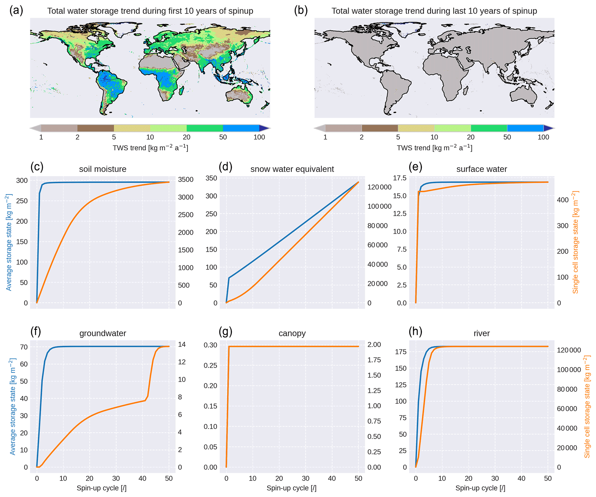
Figure 5 Evolution of various storage contents during HydroPy spin-up. The maps shows the trends in the total water storage (all storage accumulated) during the first (left map) and last (right map) 10 years of spin-up. Blue lines show values averaged over the whole land surface, and orange lines represent the grid cell with the largest residual trend at the end of the spin-up period.

Analysing the individual water storages of the spin-up simulation (see Fig. 5, blue lines), their simulated contents averaged over the land surface become stable within 10 years or less, with the exception of snow water equivalent for which single grid cells continuously accumulate snow. These cells are located close to the coasts of Greenland and Antarctica. They are not masked as their glacier fraction is smaller than the land fraction, but they have surface temperatures below 0 ^∘C for most of the year. Currently, no glacier flow processes are implemented in HydroPy, and therefore these cells cannot reach a stable state. However, this issue affects less than 2 % of the snow-covered grid cells, and these cells can easily be masked during the analysis.

The remaining storages differ in the number of years needed to reach a stable state. Small, highly dynamical storages like canopy and skin (not shown) are already well initialized during the first year, while storages with larger values and slower processes like soil moisture, groundwater and river storage show positive trends in their mean state until year 8. Thus, 50 years of spin-up seems somewhat excessive at first glance. However, the mean storage state is not necessarily representative for the whole land surface as can be demonstrated by considering the storage content for the individual grid cells that show the largest residual trend at the end of the 50-year spin-up period (Fig. 5, orange lines). In the most extreme case, soil moisture spin-up takes the major part of the 50-year period for a grid cell in the Ganges delta where the soil moisture capacity is much larger than for the majority of the other cells. Another effect is seen in the groundwater storage of a cell in the same region where a stable state was almost achieved after 40 years but was followed by a second increase period. This behaviour results from the drainage calculation (Eq. 16) whereby an exponential component is added in the case that the soil moisture exceeds a given threshold. Thus, groundwater spin-up in cells with a positive water balance and large soil moisture storage cannot be completed until the overlying soil reaches a stable state. For river storage, the most extreme cell does not spin up much slower than the average, but looking at the single-cell data, the storage content is shown to exceed those of other cells by several orders of magnitude. This cell is located at the eastern border of Lake Ontario where the main path of the St. Lawrence River crosses a grid cell with a lake fraction only slightly smaller than 1. This results in a strongly reduced flow velocity in this cell and consequently a huge water storage is built up. In summary, a shorter period of 10 years would be sufficient for most of the land surface. However, regional features clearly justify a spin-up period of 50 years. Of course, for later studies the length of spin-up simulations can be significantly reduced using restart data from another suitable HydroPy run.

4.2 Evaporation

As precipitation is provided as forcing, the major task of HydroPy is to realistically distribute precipitation into evaporation and runoff. Thus, a good representation of evaporation is crucial to successfully simulate river discharge. Unfortunately, there are no global datasets of directly observed evaporation time series available that could be used for model validation. However, data are available from the Global Land Evaporation Amsterdam Model (GLEAM; Martens et al., 2017; Miralles et al., 2011; ICDC, 2019), a sophisticated modelling system dedicated to estimating evaporative fluxes based on satellite observation and reanalysis data.

Comparing the long-term zonal mean actual evaporation between HydroPy and GLEAM (Fig. 6, upper panel) both datasets agree very well for the high and mid-latitudes in terms of zonal mean and standard deviation. However, for the tropical region between 10 and −15^∘ N HydroPy underestimates evapotranspiration by almost 1 $\mathrm{kg}{\mathrm{m}}^{-\mathrm{2}}{\mathrm{d}}^{-\mathrm{1}}$. Considering seasonal differences (Fig. 6, lower panel), some more deviations become evident. During MAM the underestimation of tropical evapotranspiration is most pronounced, affecting a band of more than 10^∘ width south of the Equator. During JJA this is compensated for by a slight overestimation south of −10^∘ N, while the evaporation underestimation shifts northwards. Also, a small (≈ 0.5 $\mathrm{kg}{\mathrm{m}}^{-\mathrm{2}}{\mathrm{d}}^{-\mathrm{1}}$) negative bias is visible between 30 and 70^∘ N.

Figure 6 Zonal mean evaporation averaged over the period 1980–2014 for HydroPy and GLEAM (a) as well as their seasonal differences in the boreal spring (MAM) and summer (JJA) (b).

While the implications of these biases for runoff are discussed in a following paragraph (see Sect. 4.3), we aim to identify possible reasons for their appearance. The most obvious source would be potential evaporation, which is provided to HydroPy as input based on atmospheric forcing data and used in every evaporation computation as a maximum value – especially as the Penman–Monteith methodology is shown to underestimate PET in tropical regions (Weiland et al., 2015). However, PET is overestimated compared to GLEAM (see Fig. 7) and thus unlikely to cause values in ET that are too low. Instead, the ET biases are well reflected in transpiration with even stronger values. This could hint at either issues with the overall size of the soil moisture storage or indicate a missing interaction between the shallow groundwater and soil moisture storages, which could provide plants with additional water for transpiration during dry periods. The importance of a deep soil moisture layer for transpiration was already demonstrated by Hagemann and Stacke (2015) and might be relevant for HydroPy as well.

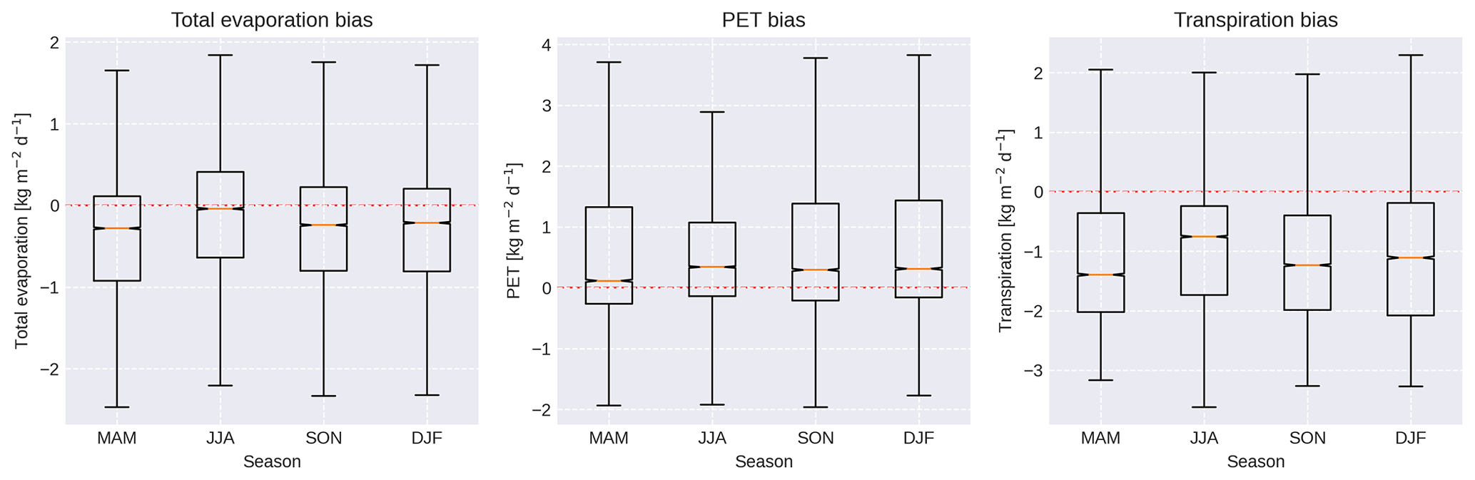
Figure 7 Percentile distribution of biases in the differences of seasonal mean fields between HydroPy and GLEAM data between 20 and −20^∘ N.

4.3 River discharge

River discharge is the most important output variable of HydroPy. It is an easily observable quantity that integrates the lateral water fluxes over a given catchment region, and it is highly sensitive to all other components of the hydrological cycle. As such, river discharge is a prime target to evaluate the skill of GHMs. This is done for the whole globe using observations provided by GRDC (2020).

We use the Kling–Gupta efficiency (KGE; Gupta et al., 2009) as a primary evaluation metric for river discharge. The KGE is defined as

$$\begin{array}{}\text{(42)}& \mathrm{KGE}=\mathrm{1}-\sqrt{{\left(r-\mathrm{1}\right)}^{\mathrm{2}}+{\left({\displaystyle \frac{{\mathit{\sigma }}_{\mathrm{sim}}}{{\mathit{\sigma }}_{\mathrm{obs}}}}-\mathrm{1}\right)}^{\mathrm{2}}+{\left({\displaystyle \frac{{\mathit{\mu }}_{\mathrm{sim}}}{{\mathit{\mu }}_{\mathrm{obs}}}}-\mathrm{1}\right)}^{\mathrm{2}}},\end{array}$$

with r being the correlation between simulated (sim) and observed (obs) river discharge time series, σ being their standard deviation, and μ being their long-term mean value. The KGE ranges in the bounds $\left\{-\mathrm{\infty },\mathrm{1}\right\}$, with a value of KGE $=-\mathrm{0.41}$ indicting a performance similar to using the observed mean flow (Knoben et al., 2019). The open lower bound complicates the comparison of KGE values between different simulations or models as their differences can become very large for catchments with unsatisfactory model performance, while changes in well capture catchments are restricted to a much smaller range. For this reason, we use a normalization when comparing KGE values following the approach used by Nossent and Bauwens (2012) for the Nash–Sutcliffe efficiency (NSE) by remapping its value range to {0,1}. We compute the difference of normalized KGE values as

$$\begin{array}{}\text{(43)}& \mathrm{\Delta }\mathrm{NKGE}={\displaystyle \frac{\mathrm{1}}{\mathrm{2}-{\mathrm{KGE}}_{{\mathrm{sim}}_{\exp }}}}-{\displaystyle \frac{\mathrm{1}}{\mathrm{2}-{\mathrm{KGE}}_{{\mathrm{sim}}_{\mathrm{ref}}}}}\end{array}$$

for all KGE comparisons.

Please note that river discharge observations are often not available directly at the river mouth. For our analysis, we use stations located at the most downstream part of the catchment and compare it with discharge from the closest grid cell with a similar inflow area. Nonetheless, the resulting values are projected onto the whole catchment for visualization. Additionally, we analyse the temporal correlation r and the percentile bias pb given by the following equations.

$$\begin{array}{}\text{(44)}& {\displaystyle }r& {\displaystyle }={\displaystyle \frac{\sum \left(Q_m-\stackrel{\mathrm{‾}}{Q_m}\right)\left(Q_o-\stackrel{\mathrm{‾}}{Q_o}\right)}{\sqrt{\sum {\left(Q_m-\stackrel{\mathrm{‾}}{Q_m}\right)}^{\mathrm{2}}\sum {\left(Q_o-\stackrel{\mathrm{‾}}{Q_o}\right)}^{\mathrm{2}}}}}\text{(45)}& {\displaystyle }\mathrm{pb}& {\displaystyle }={\displaystyle \frac{{\sum }_{t=\mathrm{1}}^T\left(Q_m^t-Q_o^t\right)\cdot \mathrm{100}}{{\sum }_{t=\mathrm{1}}^T{Q}_o^t}}\end{array}$$

Figure 8 (histogram and upper map) shows the KGE for simulated and observed data for monthly river discharge climatologies in the 100 largest catchments of the world. Only about 25 % of the catchment-covered area shows a KGE $\le -\mathrm{0.41}$, which indicates an insufficient performance, as just using the observed long-term average is superior to the prediction. Thus, HydroPy shows a reasonable performance for the majority of catchments. About 65 % of the catchment area exceeds a KGE of 0 %, and 33 % even exceeds a KGE of 0.5. Contrary to the NSE, which was often used in hydrological analysis (Moriasi et al., 2007) prior to the development of the KGE, the individual KGE values are not associated with a specific performance rating. Still, positive values are generally considered to indicate skilful model application (Knoben et al., 2019). Taking into account the fact that HydroPy is neither calibrated nor adapted to any specific catchment, its performance is satisfactory for the majority of catchments and on the same level as its predecessor MPI-HM (see Sect. 4.4).

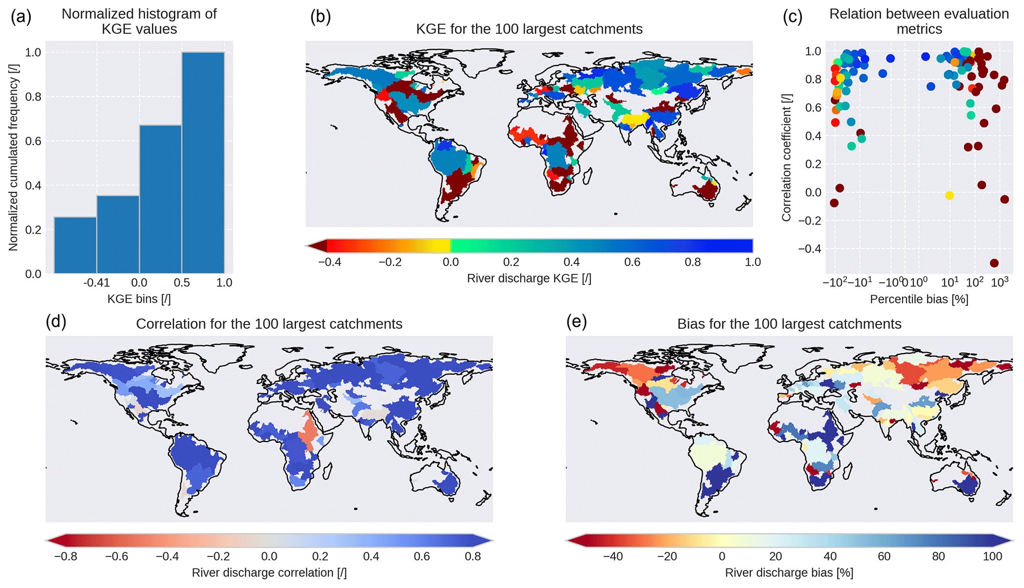
Figure 8 Kling–Gupta efficiency (KGE) of simulated river discharge climatologies for the world's 100 largest catchments compared to GRDC observations (GRDC, 2020): the upper panels show the cumulative histogram (a) of the spatial distribution (b) of KGE values and its relation (c) to the temporal correlation and percentile bias. The spatial distribution of the latter two metrics are shown in the lower panels.

Still, some river catchments could not be represented sufficiently well. Thus, additional metrics were calculated to identify reasons for this failure. Figure 8 (lower left panel) shows the temporal correlation between HydroPy and GRDC monthly mean river discharge, with a good performance for most catchments. More than two-thirds of the grid cell shows a correlation > 0.75, and less than 15 % is below 0.5. Thus, HydroPy demonstrates significant skill in representing seasonal river discharge variations in the majority of catchments. Exceptions can be seen for the Nile and Ganges rivers, which also show low KGE values. Stronger regional discrepancies are evident for the percentile bias between HydroPy and GRDC river discharge (Fig. 8, lower right panel). Only 20 % of the grid cells fall in the range of ±10 % bias. For high-northern-latitude catchments, a strong underestimation of river discharge is visible, especially for eastern Siberia and north-western Canada. Strong discharge overestimation is found for many dry regions in the Sahel zone and Australia, but also in parts of South America. Combining these measures (Fig. 8, upper right panel) shows that low KGE values occur mostly in regions with strong positive biases in mean discharge amounts and hence in total runoff. Therefore, this needs to be a focus of future model development. However, it might be possible that not all of these issues can be addressed by the model alone. Figure 9 shows the long-term water balance residuum based on GSWP3 precipitation, GLEAM evaporation and GRDC river discharge. While it is only a first-order approximation using a mixture of observed and computed quantities, it also highlights large negative values for eastern Siberia and north-western Canada as well as positive values for parts of South America, the Sahel zone and the Ganges basin. The wet bias areas coincide especially well with the regions showing strong river discharge biases in HydroPy. This points to the possibility that the forcing or validation data might already suffer from uncertainties and thus contribute to the diagnosed river discharge biases for the these regions.

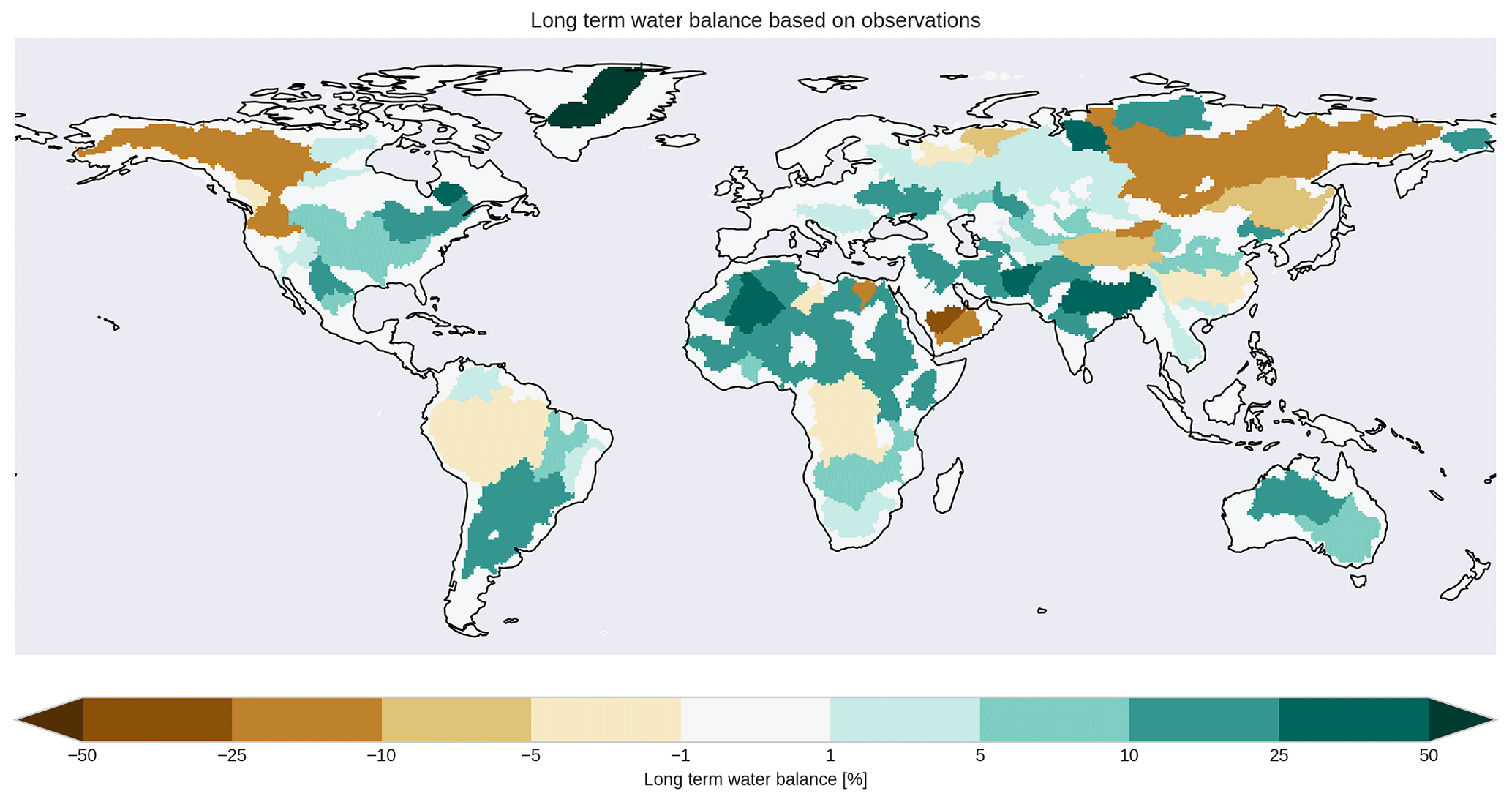
Figure 9 Long-term water balance based on GSWP3 precipitation, GLEAM evaporation and GRDC river discharge remapped to catchment scale. Note that this water balance is only a first-order estimate. No trends in storage content are included. Furthermore, the GRDC river discharge climatologies often represent different time periods than GSPW3 and GLEAM.

For regional river discharge curves (see Fig. 10), it can be seen that for Arctic rivers the peak flow month is represented very well, but the amount of peak flow is underestimated even though ET is too low during summer. In terms of model skill, this could be related to too little accumulated snow cover during the winter months. Also, during August and September, the discharge stays below the observed level. Whether this is an effect of water storages in the soil that are too small, biases in the model forcing or other processes needs to be examined in later studies. For tropical rivers, a flow peak that is too early combined with too much discharge is visible. This can be attributed mostly to the strong negative ET bias during MAM and might also be related to the missing representation of interactive floodplains, which might enhance ET and mitigate the peak flow. However, it should be noted that the discharge curve is strongly dominated by the Amazon and Congo, while other tropical rivers, like the Orinoco, Mekong and Rio Magdalena, are much better simulated. Similarly, river discharges for mid-latitude regions like the European rivers are represented very well by HydroPy.

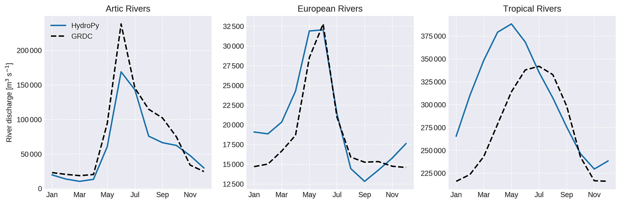
Figure 10 Climatological river discharge curves averaged for selected rivers in three regions: Arctic rivers (Lena, Ob, Yenisey, Amur, Kolyma, Mackenzie River and Yukon), European rivers (Danube, Rhine, Rhone, Po, Vistula, Pechora and Neva) and tropical rivers (Amazon, Congo, Orinoco, Mekong, Rio Magdalena, Zambezi and Niger). Simulated HydroPy discharge curves are indicated in blue, and GRDC observations are in dashed black.

4.4 Comparison to MPI-HM

In this section, HydroPy is compared to the original MPI-HM to prove its suitability as a successor. For this purpose, a simulation was conducted with MPI-HM using the same meteorological forcing data and spin-up duration. Similar to HydroPy, MPI-HM includes a number of grid cells with steadily increasing snow storage. These cells were masked during the analysis of both simulations.

Figure 11 shows the average water fluxes and storage contents for HydroPy and MPI-HM. As expected, both are rather similar. The average precipitation received by the models amounts to a yearly sum of ≈ 760 $\mathrm{kg}{\mathrm{m}}^{-\mathrm{2}}{\mathrm{a}}^{-\mathrm{1}}$. Evapotranspiration in HydroPy exceeds the one in MPI-HM by ≈ 20 $\mathrm{kg}{\mathrm{m}}^{-\mathrm{2}}{\mathrm{a}}^{-\mathrm{1}}$, while total runoff is ≈ 11 $\mathrm{kg}{\mathrm{m}}^{-\mathrm{2}}{\mathrm{a}}^{-\mathrm{1}}$ lower. The soil moisture storage is around ≈ 12 kg m⁻² higher in MPI-HM compared to HydroPy. Although both models agree in the spatial distribution of soil moisture trends, the drying trends are slightly stronger in the HydroPy simulation, resulting in an overall lower soil moisture. The average snow water equivalent is similar in both models with a difference of < 1 kg m⁻². Still, regional differences can be found featuring an increase in snow cover in the high northern latitudes (due to later snowmelt) balanced by a decrease in mid-latitudes. These small differences can be explained by the new processes implemented in HydroPy. The addition of skin and canopy evaporation increases overall evapotranspiration in HydroPy, resulting in a slight decrease in soil moisture and therefore a decrease in total runoff. The differences in SWE are caused by the replacement of the normalized sinus function in the snowmelt scheme with an explicit calculation of the day-length fraction.

Figure 11 Land surface water fluxes (a) and storage states (b) averaged over the simulation period for HydroPy (blue) and MPI-HM (orange).

Comparing the quality of simulated river discharge between the two models (see Fig. 12), HydroPy shows slightly better results in the normalized Kling–Gupta efficiency (NKGE) for about 60 % of the area of considered catchments. While the changes in NKGE values are mostly small, there are some catchments with stronger signals, e.g. the Ganges–Brahmaputra, Yangtze and Yenisey. Climatologies for the three rivers are shown in the upper panels of Fig. 13. For these basins, HydroPy generates a delay in river flow compared to MPI-HM and GRDC observations, which results in a later peak flow by 1 to 2 months and an overall smoother curve. This behaviour results from the representation of surface water in HydroPy and its effect on river flow velocity. Indeed, the wetland masks used in both models differ. MPI-HM relied on a wetland distribution compiled by Matthews and Fung (1987). However, this dataset is only available at the rather low resolution of 1^∘. In order to enable HydroPy to run on resolutions higher than the default 0.5^∘ in future applications, lakes and wetlands are now compiled using the GLWD (Lehner and Döll, 2004, see Sect. 3), which is available at 5^′ resolution. While both maps agree on the general distribution of wetlands, there are regional differences. Most prominently, the Matthews and Fung (1987) dataset contains fewer wetlands than the GLWD in the Ganges delta, the downstream area of the Yangtze River and the outlet of the Yenisey, which results in the overestimation of wetland impacts in HydroPy. The same effect causes the increase in NKGE for the Mississippi and Yukon catchments (see Fig. 13, middle panels) where HydroPy reproduces the timing of the peak flow much better than MPI-HM, although it falls off too quickly during the summer in the case of the Yukon. Here, the wetland impact acts too strongly in MPI-HM, while the selection of GLWD wetland classes in HydroPy leads to fewer wetlands in this area. Another example demonstrating the small differences between HydroPy and MPI-HM is the improved river discharge in the Danube catchment. Here, the small changes in the snow scheme slightly reduce the snow cover and thereby the snowmelt peak.

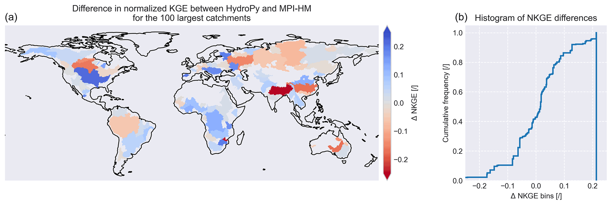
Figure 12 Spatial distribution (a) and cumulative histogram (b) of NKGE differences for river discharge between HydroPy and MPI-HM.

The river discharge simulation for Ganges–Brahmaputra, Yangtze and Yenisey can be significantly improved in HydroPy by adapting the reference flow velocity for wetlands (see Fig. 13, lower panel). However, the effect is diametrical to the skill in other wetland-influenced catchments. An increase in the reference velocity reduces the wetland impact, thereby improving the simulation skill towards the level of MPI-HM. At the same time, it results in performance degradation in other catchments like the Ob, where due to the faster river flow through wetlands the snowmelt peak appears earlier in the year, while too little water is available during late summer.

Besides exploring the reasons behind differences between HydroPy and MPI-HM, this analysis demonstrates the strong sensitivity of river discharge to wetland extent in both models. However, the opposing effects of modifying the wetland reference flow velocities discourages any further attempts to optimize this value at this point. More likely, better results can be obtained at higher resolution when flow paths and wetland distribution are represented in greater detail. Then, only wetlands which are indeed close enough to the flow channel and not simply in the same 0.5^∘ grid cell would mitigate river discharge.

Finally, it should be noted that due to the active participation of MPI-HM in several intercomparison projects (e.g. Haddeland et al., 2011; Zhang et al., 2017; Gädeke et al., 2020), there are many analyses available that evaluate the performance of MPI-HM in comparison to other GHMs. As MPI-HM and HydroPy produce very similar results, these analyses are also a good indication for the performance of HydroPy at this stage of development.

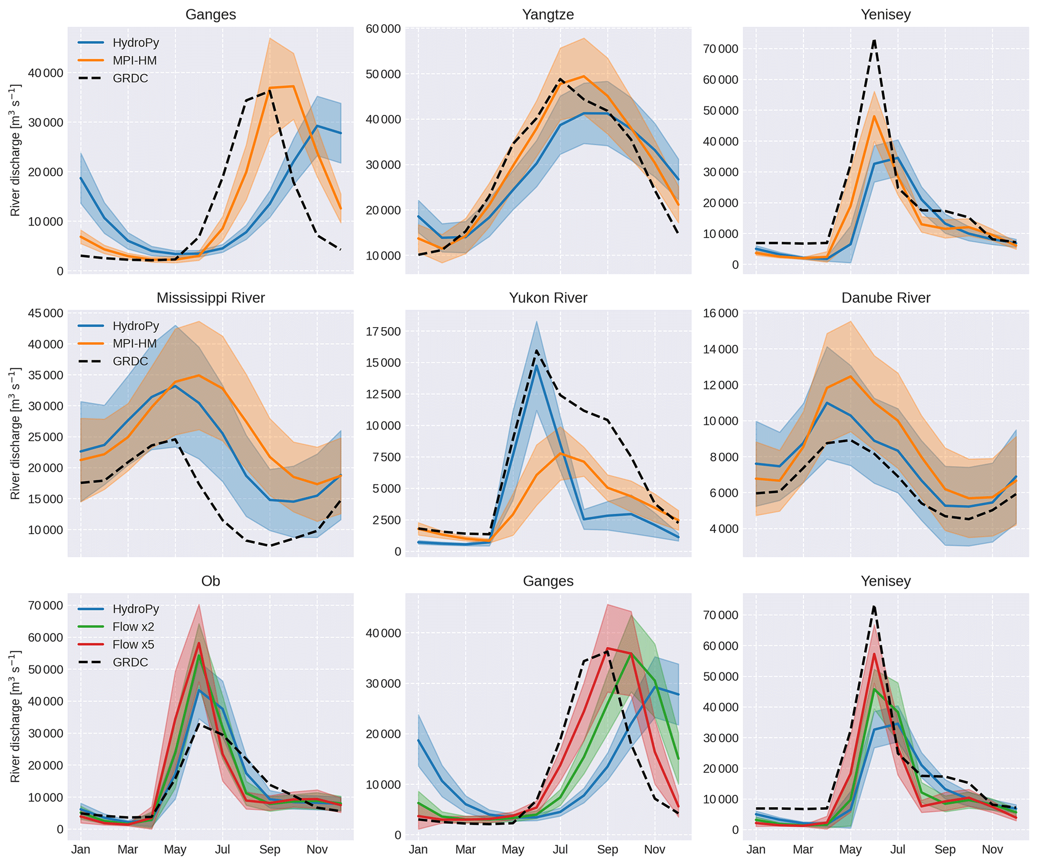
Figure 13 Monthly climatologies of river discharge for different river catchments with GRDC observations (dashed black). The upper two rows also show simulated discharge from HydroPy (blue) and MPI-HM (orange). The lower row shows simulated river discharge produced with the default parameters in HydroPy (blue) as well as those with modified reference flow velocities for wetlands using factors of 2 (green) and 5 (red).

5 Conclusions

This study introduces HydroPy, a global hydrological model written in Python. Similar to its predecessor, the MPI-HM, the model simulates the land surface water balance as well as the river routing towards the ocean. HydroPy uses a default resolution of 0.5^∘ on a global scale. It has rather humble data requirements, using surface temperature, precipitation and potential evaporation as meteorological input data together with land surface property data. Compared to MPI-HM, HydroPy can be set up more easily, has fewer requirements for land surface data, provides internal checks to aid the model development process and requires less effort for maintenance and implementation of new processes.

The majority of process formulations were taken over from MPI-HM without any alterations, but some improvements were done for the snowmelt, the skin and canopy storages, and the impact of lakes and wetlands on river discharge. The evaluation of evapotranspiration using the GLEAM data (Martens et al., 2017; Miralles et al., 2011; ICDC, 2019) shows a generally reasonable behaviour but also highlights underestimation of transpiration in parts of the tropics and the high northern latitudes. This affects runoff generation and results in an overestimation of river discharge, especially for the Amazon and Congo rivers, compared to GRDC data (GRDC, 2020) and also a discharge peak that is too early for these two rivers. The seasonality of Arctic rivers is captured very well, but the peak discharge is generally too low. Although constraint to specific regions, both biases are considered to be important deficiencies – either in the model or in the meteorological forcing data – and will be a focus of the next development steps. Still, the majority of catchments show a very good correlation with observations, and overall discharge can be satisfactorily represented by HydroPy.

Besides the necessary improvements in these parameterizations, there are further plans to actively develop HydroPy in the future. The two most important focus areas are the

• transport of nutrients within the lateral flow scheme of HydroPy to provide ocean models not only with river discharge, but also transient information about nutrient concentration, and

• implementation of human impacts, especially irrigation and crop management, but also the representation of dams and reservoirs.

Compared to MPI-HM, HydroPy shows very similar results on the global scale. However, there are regional differences due to changes in the snowmelt scheme and the updated wetland distribution. While these changes cause a degraded performance of river discharge in a few river basins, the majority of rivers benefit from the improvements implemented in HydroPy. Nonetheless, regions with decreased simulation quality will be the focus of further model development. In conclusion, the transition from MPI-HM to HydroPy is completed successfully and HydroPy will replace MPI-HM in future applications.

As final remarks we present some insights gained during this project. Naturally, HydroPy is not the first hydrology model to be rewritten (e.g. SWAT+; Bieger et al., 2016, and others); however, the difficulties and challenges of such a project are not often discussed (Müller et al., 2018). A major obstacle is the perception of this work: rewriting a model prepares the way for new studies but is often considered a technical rather than a scientific task. For this reason, it is difficult to secure funding, computational resources and finally publish this work in high-ranking journals. As scientists are often employed on limited contracts, they need to carefully weigh such time investments because model development, maintenance and documentation usually pay off only on long timescales. For this reason, small working groups without technical support are at a disadvantage when trying to rewrite their models. Still, in terms of the technical realization, we would like to share some advice that was useful to us.

• Programming language and style should be chosen according to the user base and application, e.g. Fortran or C for highly optimized models running on high-performance machines vs. interpreted languages like Python or R with easily understandable code for educational purposes or working groups without technical support staff.

• Infrastructural routines should be separated from the scientific code as much as possible. If I/O and variable definitions happen “under the hood”, the main routine can be much more easily understood and extended by other scientists. For this very reason, we recommend developing the model infrastructure as the very first step and only later adding the scientific processes.

• Implement automated checks right from the beginning. Standardized computations of water and mass balances as well as sensible additional outputs, e.g. log outputs for selected grid cells, help to spot any conceptual or programming errors as early as possible.

• Port one routine at a time and summarize related functions in one file for a better overview. A modular model can be much more easily extended for different applications.

• Write documentation right from the start and not only when the first model version is finished.

• Use a versioning tool (git, svn) to manage the development progress, collaborations and releases.

Of course, all this advice comes from personal preferences and other programmers might set different priorities. Nonetheless, we hope it might ease the start on such projects because, ultimately, a well-structured and maintained open-source model is a valuable asset in hydrological research.