ChAP 1.0: a stationary tropospheric sulfur cycle for Earth system models of intermediate complexity

A stationary, computationally efficient scheme ChAP 1.0 (Chemical and Aerosol Processes, version 1.0) for the sulfur cycle in the troposphere is developed. This scheme is designed for Earth system models of intermediate complexity (EMICs). The scheme accounts for sulfur dioxide emissions into the atmosphere, its deposition to the surface, oxidation to sulfates, and dry and wet deposition of sulfates on the surface. The calculations with the scheme are forced by anthropogenic emissions of sulfur dioxide into the atmosphere for 1850–2000 adopted from the CMIP5 dataset and by the ERA-Interim meteorology assuming that natural sources of sulfur into the atmosphere remain unchanged during this period. The ChAP output is compared to changes of the tropospheric sulfur cycle simulations with the CMIP5 data, with the IPCC TAR ensemble, and with the ACCMIP phase II simulations. In addition, in regions of strong anthropogenic sulfur pollution, ChAP results are compared to other data, such as the CAMS reanalysis, EMEP MSC-W, and individual model simulations. Our model reasonably reproduces characteristics of the tropospheric sulfur cycle known from these information sources. In our scheme, about half of the emitted sulfur dioxide is deposited to the surface, and the rest is oxidised into sulfates. In turn, sulfates are mostly removed from the atmosphere by wet deposition. The lifetimes of the sulfur dioxide and sulfates in the atmosphere are close to 1 and 5 d, respectively. The limitations of the scheme are acknowledged, and the prospects for future development are figured out. Despite its simplicity, ChAP may be successfully used to simulate anthropogenic sulfur pollution in the atmosphere at coarse spatial scales and timescales.

1 Introduction

Sulfur compounds in the troposphere are important pollutants and contribute both to the direct radiative effect, which is also known as an aerosol–radiation interaction, and, owing to their hygroscopicity, are major contributors to the aerosol indirect effects on climate – the so-called aerosol–cloud interaction (Charlson et al., 1992; Boucher et al., 2013). The direct radiative forcing from the pre-industrial period up to the 2010s is estimated to amount from −0.2 to −0.8 W m⁻² (Boucher et al., 2013; Myhre et al., 2013; Shindell et al., 2013; Zelinka et al., 2014; Matus et al., 2019). The sulfate contribution to aerosol–cloud interaction leads to the corresponding indirect forcing from −0.2 to $-\mathrm{1.2}\mathrm{W}{\mathrm{m}}^{-\mathrm{2}}$ (Zelinka et al., 2014; McCoy et al., 2017). These forcings arise from the anthropogenic release of sulfates and of sulfur precursors (mostly of sulfur dioxide, SO₂).

Apart from influencing climate change, sulfur compounds impact terrestrial vegetation and thus the global carbon cycle. The first effect is due to suppression of the terrestrial vegetation gross primary production arising from the uptake of sulfur dioxide by leaves with subsequent injury of photosynthesis tissues of plants (Semenov et al., 1998). This suppression may be as large as 10 % relative to the SO₂-unaffected plants, especially in moist tropical forests (Eliseev, 2015a, b; Eliseev et al., 2019). Another impact is due to acidification of soils and surface waters with a risk of vegetation poisoning (Kuylenstierna et al., 2001).

There are a number of chemically active sulfur species in the Earth's atmosphere. Among these species, the most abundant are sulfur dioxide SO₂, which is either oxidised from precursors such as dimethyl sulfide (DMS), hydrogen sulfide H₂S, and carbon disulfide CS₂; emitted by volcanos; or released due to anthropogenic activity (Seinfeld and Pandis, 2006; Warneck, 2000; Surkova, 2002). An additional minor SO₂ source is due to biomass burning. Less abundant but still important in global sulfur cycle are dimethyl sulfide, dimethyl sulfoxide (DMSO), and methanesulfonic acid (MSA). All of these species chemically interact with each other and undergo wet and dry deposition on the Earth's surface. As a whole, a chemical reaction chain converts sulfur compounds into sulfur dioxide, which is further oxidised into sulfuric acid H₂SO₄ and sulfates ${\mathrm{SO}}_{\mathrm{4}}^{\mathrm{2}-}$ (Seinfeld and Pandis, 2006; Warneck, 2000; Surkova, 2002).

All of this has motivated researchers to implement interactive sulfur cycle into global climate models (or, more precisely, into Earth system models, ESMs). Starting from the pioneering paper by Chatfield and Crutzen (1984), research groups from different modelling centres included sulfur cycles into their ESMs. The most active phase of these projects was in late 1980s and 1990s, which resulted in a number of chemical transport models that may be or may be not coupled to ESMs: MOGUNTIA (Langner and Rodhe, 1991), IMAGES (Pham et al., 1995), ECHAM (Feichter et al., 1996; Roelofs et al., 1998), Harvard-GISS (Koch et al., 1999), CCM1-GRANTOUR (Chuang et al., 1997), CCM3 (Barth et al., 2000; Rasch et al., 2000), CCCMA (Lohmann et al., 1999), and GOCART (Chin et al., 2000). These models were summarised in the Intergovernmental Panel on Climate Change Third Assessment Report (IPCC TAR) (Houghton et al., 2001, their Table 5.8). Later, these models became able to account for other types of aerosol and interaction between different geochemical cycles (Forster et al., 2007; Boucher et al., 2013), which led to the development of the AeroCom and ACCMIP (Atmospheric Chemistry and Climate Model Intercomparison Project) activities, (Shindell et al., 2013; Lamarque et al., 2013a; Myhre et al., 2013; Tsigaridis et al., 2014; Fiedler et al., 2019; Riemer et al., 2019; Bellouin et al., 2020; Gliß et al., 2021).

In parallel, a number of the reduced-complexity, computationally cheap ESMs, which are collectively referred to as Earth system models of intermediate complexity (EMICs), have emerged (Claussen et al., 2002; Petoukhov et al., 2005; Eby et al., 2013; Zickfeld et al., 2013; MacDougall et al., 2020). These models are mostly targeted for simulations at coarse (e.g. subcontinental) spatial scales but are run either for very long time intervals or for large ensemble simulations (e.g. Eby et al., 2009; Collins et al., 2011; Eliseev, 2011; Willeit et al., 2014; MacDougall and Knutti, 2016; Ganopolski and Brovkin, 2017; Muryshev et al., 2017). One may argue that such models also need modules to mimic atmospheric chemistry. For instance, lacking an interactive atmospheric sulfur cycle, EMICs attempt to simulate 20th century climate changes ignoring radiative forcing from tropospheric sulfates. This hampers an evaluation of the realism of the models of this type. At time of writing, there are only two EMICs that have implemented radiative forcing from sulfates: IAPRAS-MSU (A.M. Obukhov Institute of the Atmospheric Physics, Russian Academy of Sciences – Lomonosov Moscow State University) (Eliseev et al., 2007) and Climber-2 (Bauer et al., 2008).

The latter model also implements a very simple atmospheric sulfur cycle scheme in which sulfate burden per unit area is related to their precursor emissions at the same grid cell by using a prescribed coefficient, which, in turn, is related to atmospheric lifetimes of sulfates and their precursors taking into account that part of the emitted precursors are deposited before they are oxidised into sulfates. No horizontal transport of sulfates and their chemical precursors is allowed for. This approach is reasonable for Climber-2 with its very coarse horizontal resolution (10^∘ by latitude and 51.3^∘ by longitude, Bauer et al., 2008) but becomes problematic for other EMICs in which this resolution is higher.

A somewhat similar but inverse approach was pursued in the IAPRAS-MSU model. In this model, SO₄ burden is prescribed as a function of time, and SO₂ burden is reconstructed by using an atmospheric moisture-dependent coefficient to calculate the SO₂ impact on terrestrial gross primary production (Eliseev et al., 2019).

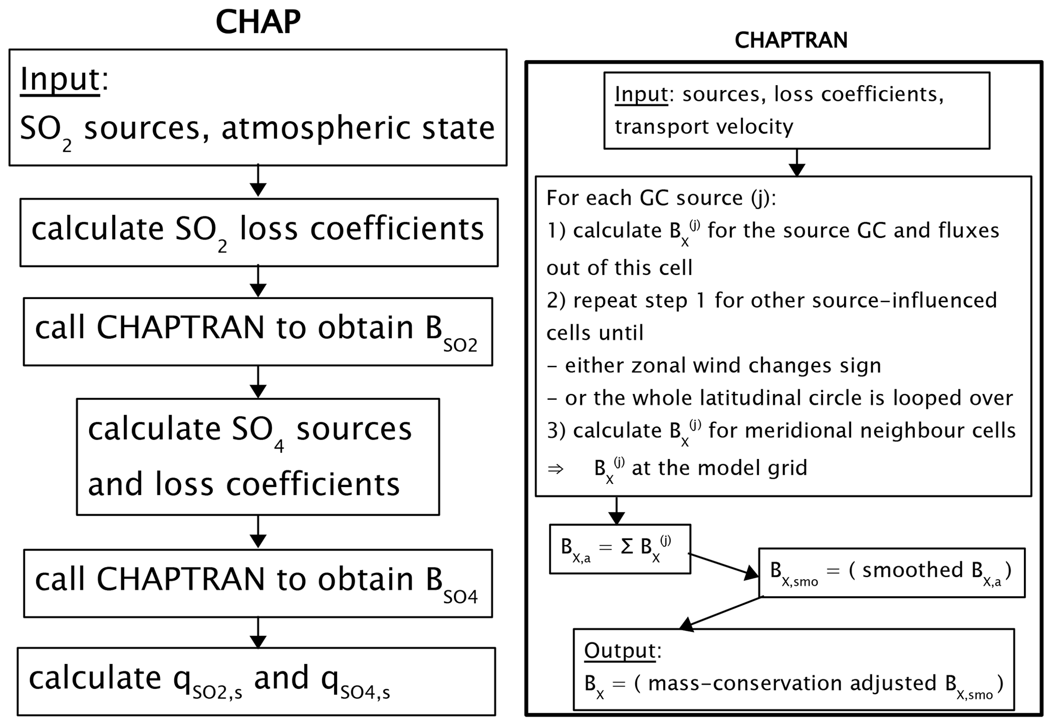
The goal of the present paper is to make a step beyond the Climber-2 and IAPRAS-MSU approaches and to allow for transport of sulfur species in the horizontal direction and the calculation of characteristics of the sulfur cycle directly. This should be done in a computationally efficient manner in order not to destroy an important property of EMICs – their small turnaround time. This precludes usage of the sulfur cycle scheme implemented into the above-mentioned chemical transport models. Thus, we developed a stationary scheme, ChAP (Chemistry and Aerosol Processes), which is able to mimic gross dynamics of the atmospheric chemistry. Its contemporary version, ChAP 1.0, implements only the anthropogenic part of the atmospheric sulfur cycle, but we plan to extend the scheme in future.

Below, a theoretical background for our scheme is presented and its offline performance is tested.

2 Scheme description

2.1 General considerations

We start from the general equations governing mass concentrations of SO₂ ($q_{{\mathrm{SO}}_{\mathrm{2}}}$) and SO₄ ($q_{{\mathrm{SO}}_{\mathrm{4}}}$) (Seinfeld and Pandis, 2006; Warneck, 2000; Surkova, 2002):

$$\begin{array}{rl}{\displaystyle \frac{\partial q_{{\mathrm{SO}}_{\mathrm{2}}}}{\partial t}}+\mathit{U}\cdot \mathrm{\nabla }{q}_{{\mathrm{SO}}_{\mathrm{2}}}=& e_{{\mathrm{SO}}_{\mathrm{2}}}+r_{{\mathrm{SO}}_{\mathrm{2}},\text{prod}}-r_{\text{in-cl}}-r_{\text{gas}}\\ & -d_{{\mathrm{SO}}_{\mathrm{2}},\text{dry}}-d_{{\mathrm{SO}}_{\mathrm{2}},\text{wet}}+a_{{\mathrm{SO}}_{\mathrm{2}}},\end{array}$$

$$\begin{array}{}\text{(1)}& \begin{array}{rl}{\displaystyle \frac{\partial q_{{\mathrm{SO}}_{\mathrm{4}}}}{\partial t}}+\mathit{U}\cdot \mathrm{\nabla }{q}_{{\mathrm{SO}}_{\mathrm{4}}}=& e_{{\mathrm{SO}}_{\mathrm{4}}}+r_{\text{in-cl}}+r_{\text{gas}}-d_{{\mathrm{SO}}_{\mathrm{4}},\text{dry}}\\ & -d_{{\mathrm{SO}}_{\mathrm{4}},\text{wet}}+a_{{\mathrm{SO}}_{\mathrm{4}}},\end{array}\end{array}$$

where e_Y is emission rate for substance Y ($Y\in \mathit{\{}{\mathrm{SO}}_{\mathrm{2}},{\mathrm{SO}}_{\mathrm{4}}\mathit{\}}$), U is three-dimensional transport velocity, r_in-cl and r_gas are, respectively, in-cloud and gas-phase oxidation converting SO₂ to SO₄, $r_{{\mathrm{SO}}_{\mathrm{2}},\text{prod}}$ is chemical SO₂ production rate in the atmosphere, d_Y,dry and d_Y,wet are dry and wet deposition rates for substance Y, respectively, and a_Y shows diffusive and convective redistribution of Y.

Because our goal is to develop a scheme for sufficiently large time steps, we assume that vertical profiles of both substances are universal in the sense that q_Y at each altitude (as well as the total burden of Y) depends only on the respective surface value. We assume an exponential dependence of q_Y on geometrical altitude (thus, explicitly excluding stratospheric sulfur compounds) with the vertical scale H_Y, which is on the order of 1 km (Jaenicke, 1993; Warneck, 2000). The latter leads to the relation between the near-surface mass concentrations q_Y,s and the total burden B_Y of substance Y per unit area:

$$\begin{array}{}\text{(2)}& B_Y=q_{Y,\mathrm{s}}{H}_Y.\end{array}$$

This allows us to integrate (1) over vertical coordinates formally from the surface up to infinity. To simplify the setup, we neglect the dependence of horizontal velocity on the vertical coordinate. The resulting equations read

$$\begin{array}{ll}{\displaystyle \frac{\partial B_{{\mathrm{SO}}_{\mathrm{2}}}}{\partial t}}+\mathit{U}\cdot \mathrm{\nabla }{B}_{{\mathrm{SO}}_{\mathrm{2}}}=& {\displaystyle }{E}_{{\mathrm{SO}}_{\mathrm{2}}}+R_{{\mathrm{SO}}_{\mathrm{2}},\text{prod}}-R_{\text{in-cl}}-R_{\text{gas}}\\ {\displaystyle }& {\displaystyle }-D_{{\mathrm{SO}}_{\mathrm{2}},\text{dry}}-D_{{\mathrm{SO}}_{\mathrm{2}},\text{wet}}+A_{{\mathrm{SO}}_{\mathrm{2}}},\\ {\displaystyle \frac{\partial B_{{\mathrm{SO}}_{\mathrm{4}}}}{\partial t}}+\mathit{U}\cdot \mathrm{\nabla }{B}_{{\mathrm{SO}}_{\mathrm{4}}}=& {\displaystyle }{E}_{{\mathrm{SO}}_{\mathrm{4}}}+R_{\text{in-cl}}+R_{\text{gas}}\\ \text{(3)}& {\displaystyle }& {\displaystyle }-D_{{\mathrm{SO}}_{\mathrm{4}},\text{dry}}-D_{{\mathrm{SO}}_{\mathrm{4}},\text{wet}}+A_{{\mathrm{SO}}_{\mathrm{4}}},\end{array}$$

where $Y\in \mathit{\{}{\mathrm{SO}}_{\mathrm{2}},{\mathrm{SO}}_{\mathrm{4}}\mathit{\}}$,

$$\begin{array}{ll}{\displaystyle }{E}_Y=& {\displaystyle }\underset{\mathrm{0}}{\overset{\mathrm{\infty }}{\int }}{e}_Y\mathrm{d}z,\\ {\displaystyle }{R}_{Y,Z}=& {\displaystyle }\underset{\mathrm{0}}{\overset{\mathrm{\infty }}{\int }}{r}_{Y,Z}\mathrm{d}z;Z\in \left\{\text{prod},\text{in-cl},\text{gas}\right\},\\ {\displaystyle }{D}_{Y,Z}=& {\displaystyle }\underset{\mathrm{0}}{\overset{\mathrm{\infty }}{\int }}{d}_{Y,Z}\mathrm{d}z;Z\in \left\{\text{wet},\text{dry}\right\},\\ {\displaystyle }{A}_{Y,Z}=& {\displaystyle }\underset{\mathrm{0}}{\overset{\mathrm{\infty }}{\int }}{a}_Y\mathrm{d}z.\end{array}$$

Equation (3) is similar to Eq. (1) with two important differences: here U is two-dimensional (we choose it at a representative altitude) and A_Y represents only the horizontal diffusion.

Further, we assume that major chemical reactions follow the common first-order kinetics relative to the source compounds. In a similar fashion, we assume that sink terms are proportional to the respective burdens. All this leads to

$$\begin{array}{ll}{\displaystyle }{R}_{\text{in-cl}}=& {\displaystyle }{k}_{\text{in-cl}}{B}_{{\mathrm{SO}}_{\mathrm{2}}},\\ {\displaystyle }{R}_{\text{gas}}=& {\displaystyle }{k}_{\text{gas}}{B}_{{\mathrm{SO}}_{\mathrm{2}}},\\ \text{(4)}& {\displaystyle }{D}_{Y,Z}=& {\displaystyle }{k}_{Y,Z}{B}_Y,Y\in \left\{{\mathrm{SO}}_{\mathrm{2}},{\mathrm{SO}}_{\mathrm{4}}\right\};Z\in \left\{\text{wet},\text{dry}\right\}).\end{array}$$

Here ks stand either for the respective reaction rate constants or for the loss rate coefficients.

Based on Warneck (2000) and on individual model simulations summarised in Houghton et al. (2001, their Table 5.5), we neglect the following terms in Eq. (1):

• both non-stationary terms $\partial B_Y/\partial t$;

• chemical SO₂ production in the atmosphere, i.e. $R_{{\mathrm{SO}}_{\mathrm{2}},\text{prod}}=\mathrm{0}$ (this assumption basically removes part of the natural sources of sulfur dioxide, e.g., the DMS oxidation);

• gas-phase sulfur dioxide oxidation, i.e. R_gas=0;

• wet deposition of sulfur dioxide, i.e. $D_{{\mathrm{SO}}_{\mathrm{2}},\text{wet}}=\mathrm{0}$ (or, equivalently, $k_{{\mathrm{SO}}_{\mathrm{2}},\text{wet}}=\mathrm{0}$).

This and the previous assumption sets makes Eq. (3) linear with respect to prognostic variables. For the time being, we additionally drop diffusion terms A_Y. Thus, Eq. (3) is reduced to

$$\begin{array}{ll}{\displaystyle }& {\displaystyle }\mathit{U}\cdot \mathrm{\nabla }{B}_{{\mathrm{SO}}_{\mathrm{2}}}=E_{{\mathrm{SO}}_{\mathrm{2}}}-k_{{\mathrm{SO}}_{\mathrm{2}}}{B}_{{\mathrm{SO}}_{\mathrm{2}}},\\ \text{(5)}& {\displaystyle }& {\displaystyle }\mathit{U}\cdot \mathrm{\nabla }{B}_{{\mathrm{SO}}_{\mathrm{4}}}=k_{\text{in-cl}}{B}_{{\mathrm{SO}}_{\mathrm{2}}}-k_{{\mathrm{SO}}_{\mathrm{4}}}{B}_{{\mathrm{SO}}_{\mathrm{4}}}.\end{array}$$

Here $k_{{\mathrm{SO}}_{\mathrm{2}}}=k_{\text{in-cl}}+k_{{\mathrm{SO}}_{\mathrm{2}},\text{dry}}$, $k_{{\mathrm{SO}}_{\mathrm{4}}}=k_{{\mathrm{SO}}_{\mathrm{4}},\text{dry}}+k_{{\mathrm{SO}}_{\mathrm{4}},\text{wet}}$, and $E_{{\mathrm{SO}}_{\mathrm{2}}}$ is SO₂ emission rate per unit area.

For a further guide, consider a one-dimensional problem with $U=\left|u\right|=\text{const}$ and the emission localised in the interval $\mathrm{0}\le x\le L$, where x is coordinate in the direction of U and L is the horizontal source size (Jacob, 2000). Its solution is shown in Fig. S1 in the Supplement. Averaged over the $\mathrm{0}\le x\le L$ domain, the solution of Eq. (5) reads

$$\begin{array}{}\text{(6)}& \stackrel{\mathrm{‾}}{B_Y}={\displaystyle \frac{E_Y}{k_Y}}\left[\mathrm{1}-{\displaystyle \frac{\mathrm{1}}{{\mathit{\gamma }}_Y}}\left(\mathrm{1}-e^{-{\mathit{\gamma }}_Y}\right)\right],\end{array}$$

where ${\mathit{\gamma }}_Y=k_{Y}L/U$. Downwind of the emission region this solution reads

$$\begin{array}{}\text{(7)}& B_Y\left(x\right)=B_Y\left(L\right)\left[\mathrm{1}-\exp \left({\mathit{\gamma }}_Y-k_{Y}x/U\right)\right].\end{array}$$

Equation (7) specifically allows us to estimate the horizontal scale of influence for this grid cell source as follows:

$$\begin{array}{}\text{(8)}& L_Y\sim \mathrm{2}U/k_Y=\mathrm{2}U{\mathcal{T}}_Y,\end{array}$$

where ${\mathcal{T}}_Y=k_Y^{-\mathrm{1}}$ is the lifetime of species Y in the atmosphere.

An estimate of ${\mathcal{T}}_{{\mathrm{SO}}_{\mathrm{2}}}$ may be obtained from Eq. (8) by using the ERA-Interim data (Dee et al., 2011). For this dataset, the typical values of zonal u and meridional v velocities in the lower troposphere in the middle latitudes, where the SO₂ pollution is most marked, are up to 7 and 5 m s⁻¹ (Fig. S2), respectively. Because the typical SO₂ lifetime is around 1–2 d (Warneck, 2000; Surkova, 2002; Houghton et al., 2001, their Table 5.5), we can estimate $L_{{\mathrm{SO}}_{\mathrm{2}}}\sim {\mathrm{10}}^{\mathrm{3}}\mathrm{km}$ (somewhat larger in the zonal direction and somewhat smaller in the meridional one). This corresponds to a few grid cells provided that the grid cell size is several hundred kilometres.

The typical horizontal scale for SO₄, $L_{{\mathrm{SO}}_{\mathrm{4}}}$ may be estimated in a similar way. Assuming that the transport velocity is of the same order of magnitude as it was for SO₂ advection, which is justified by the similar depths of the atmospheric layers of around 1.5–2 km (Warneck, 2000) when taking 4–6 d as a typical value for ${\mathcal{T}}_{{\mathrm{SO}}_{\mathrm{4}}}$ (Warneck, 2000; Surkova, 2002; Houghton et al., 2001, their Table 5.5), we estimate $L_{{\mathrm{SO}}_{\mathrm{4}}}\sim \mathrm{5}\times L_{{\mathrm{SO}}_{\mathrm{2}}}$.

2.2 Horizontal transport

Taking into account the estimates obtained for $L_{{\mathrm{SO}}_{\mathrm{2}}}$ and $L_{{\mathrm{SO}}_{\mathrm{4}}}$ above, we may construct the transport scheme as follows.

First, we solve the Eq. (5). Because it is linear with respect to $B_{{\mathrm{SO}}_{\mathrm{2}}}$, we may consider the model grid as an array of non-interacting sulfur sources numbered as j= 1, 2, etc. To reduce the computational burden, we consider only grid cells with $E_{{\mathrm{SO}}_{\mathrm{2}}}^{\left(j\right)}\ge E_{{\mathrm{SO}}_{\mathrm{2}},\text{min}}$ and set $E_{{\mathrm{SO}}_{\mathrm{2}},\text{min}}$ to a sufficiently small, empirically chosen value (Table 1). At the source grid cell, the burden $B_{{\mathrm{SO}}_{\mathrm{2}}}^{\left(j\right)}\left({\mathit{\rho }}_j\right)$ is calculated by using Eq. (6) with Y=SO₂ and with ${\mathit{\gamma }}_{{\mathrm{SO}}_{\mathrm{2}}}=k_{{\mathrm{SO}}_{\mathrm{2}}}(\mathrm{\Delta }x/u+\mathrm{\Delta }y/v)$. Here ρ_j is the horizontal coordinates of the grid cell corresponding to the source j, $E_{{\mathrm{SO}}_{\mathrm{2}}}^{\left(j\right)}=E_{{\mathrm{SO}}_{\mathrm{2}}}\left({\mathit{\rho }}_j\right)$, Δy=ℛ_EΔϕ, Δx=ℛ_Ecos ϕΔλ, ℛ_E is the Earth's radius, ϕ is latitude, and Δϕ and Δλ are grid cell sizes in latitudinal and longitudinal directions, respectively.

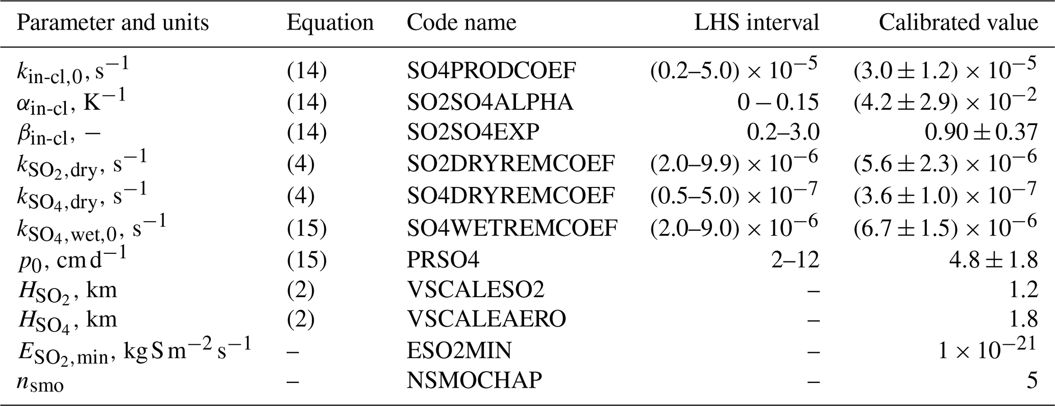
Table 1 Numerical parameters of ChAP. The symbol “–” in the column labelled “LHS interval” (where LHS is an abbreviation for Latin hypercube sampling) indicates that this parameter was not sampled during the tuning procedure, and instead the respective number from column “calibrated value” was used throughout the paper.

The difference between $E_{{\mathrm{SO}}_{\mathrm{2}}}^{\left(j\right)}$ and $k_{{\mathrm{SO}}_{\mathrm{2}}}\left({\mathit{\rho }}_j\right)B_{{\mathrm{SO}}_{\mathrm{2}}}^{\left(j\right)}\left({\mathit{\rho }}_j\right)$ is transported out of the source cell by advection:

$$\begin{array}{}\text{(9)}& F_{{\mathrm{SO}}_{\mathrm{2}},\text{out}}^{\left(j\right)}\left({\mathit{\rho }}_j\right)=E_{{\mathrm{SO}}_{\mathrm{2}}}^{\left(j\right)}-k_{{\mathrm{SO}}_{\mathrm{2}}}{B}_{{\mathrm{SO}}_{\mathrm{2}}}^{\left(j\right)}.\end{array}$$

This flux is partitioned into zonal and meridional components in proportion to the corresponding wind component and the geometric size of the corresponding boundary of the cell:

$$\begin{array}{ll}{\displaystyle }& {\displaystyle }{F}_{{\mathrm{SO}}_{\mathrm{2}},u}^{\left(j\right)}={\displaystyle \frac{u\mathrm{\Delta }y}{\left|u\mathrm{\Delta }y\right|+\left|v\mathrm{\Delta }x\right|}}{F}_{{\mathrm{SO}}_{\mathrm{2}},\text{out}}^{\left(j\right)},\\ \text{(10)}& {\displaystyle }& {\displaystyle }{F}_{{\mathrm{SO}}_{\mathrm{2}},v}^{\left(j\right)}={\displaystyle \frac{v\mathrm{\Delta }x}{\left|u\mathrm{\Delta }y\right|+\left|v\mathrm{\Delta }x\right|}}{F}_{{\mathrm{SO}}_{\mathrm{2}},\text{out}}^{\left(j\right)}.\end{array}$$

The direction of each $F_{{\mathrm{SO}}_{\mathrm{2}},u}^{\left(j\right)}\left({\mathit{\rho }}_j\right)$ and $F_{{\mathrm{SO}}_{\mathrm{2}},v}^{\left(j\right)}\left({\mathit{\rho }}_j\right)$ is determined by the direction of zonal and meridional wind, respectively.

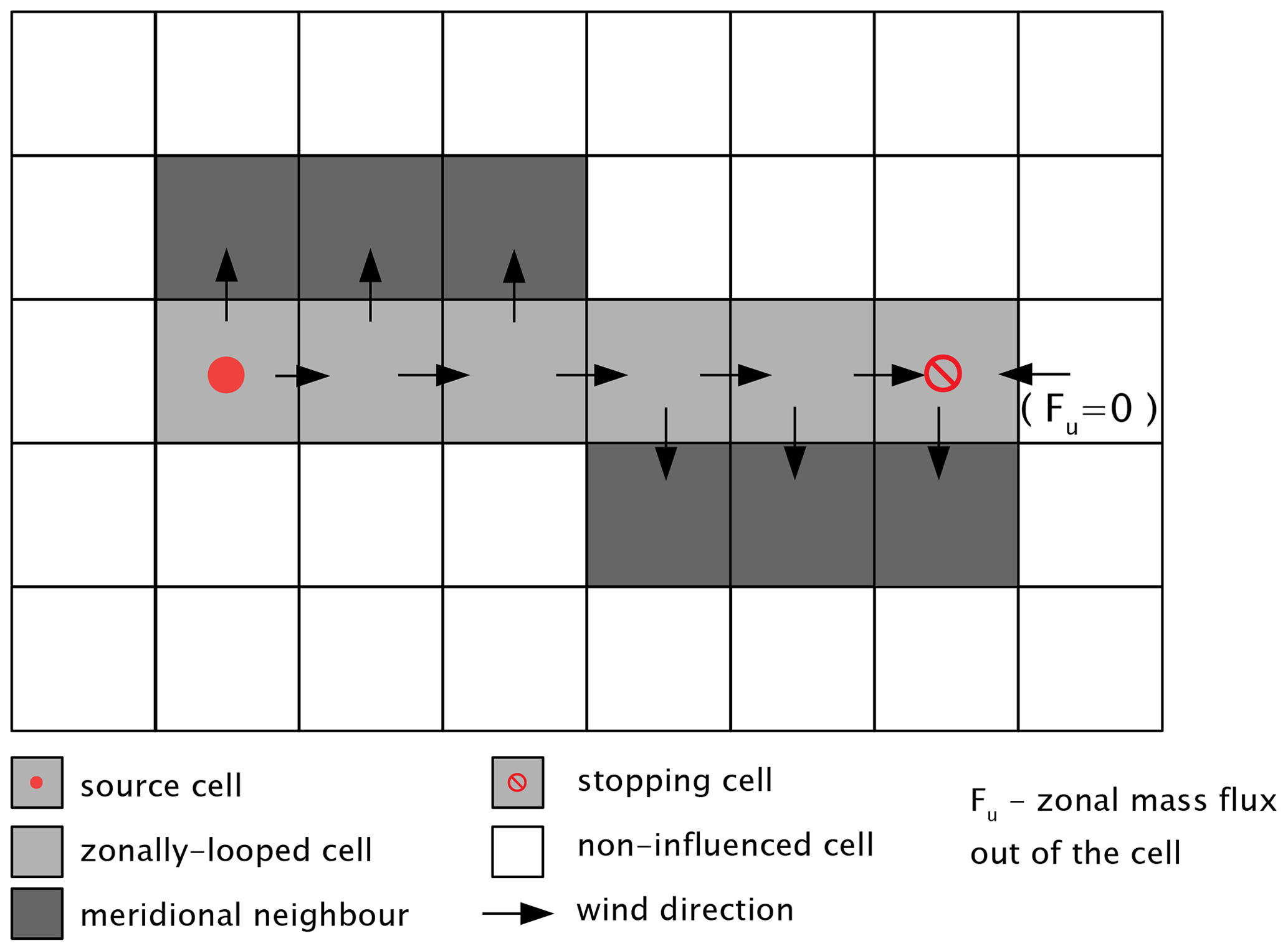
Figure 1 An illustration of advection in ChAP. Only the case when the stopping grid cell corresponds to the change of the zonal velocity sign is shown.

Then we loop in the zonal direction and calculate SO₂ burdens, related to the source j, as well as corresponding chemical and depositional losses, and fluxes out of the cell by using Eqs. (6), (9), and (10) (Fig. 1). In each cell i included in this loop, zonal flux from the previous zonal cell $F_{{\mathrm{SO}}_{\mathrm{2}},u}^{\left(j\right)}\left({\mathit{\rho }}_{i-\mathrm{1}}\right)$ is used in place of $E_{{\mathrm{SO}}_{\mathrm{2}}}^{\left(j\right)}$ and $k_{{\mathrm{SO}}_{\mathrm{2}}}\left({\mathit{\rho }}_j\right)$ is replaced by $k_{{\mathrm{SO}}_{\mathrm{2}}}\left({\mathit{\rho }}_i\right)$. The loop is stopped in the cell with the number I_(j) at which any of the following conditions is met:

• either zonal wind $u\left({\mathit{\rho }}_{I_{\left(j\right)}}\right)$ changes sign relative to u(ρ_j)

• or the whole latitudinal circle is looped over.

In the stopping cell, $F_{{\mathrm{SO}}_{\mathrm{2}},\text{out}}^{\left(j\right)}\left({\mathit{\rho }}_{I_{\left(j\right)}}\right)=F_{{\mathrm{SO}}_{\mathrm{2}},v}^{\left(j\right)}\left({\mathit{\rho }}_{I_{\left(j\right)}}\right)$.

The SO₂ mass, which is advected from the source cell and from the each of the looped-over cells, is transported to the respective neighbour cell either to the north or to the south depending on sign of v(ρ_i). No advection of sulfur dioxide mass from this meridional neighbour cell is allowed, and the SO₂ burden is calculated assuming the balance between meridional mass inflow and chemical loss (Fig. 1).

At the next step, the SO₂ burden in each grid cell is obtained by summing over all grid cell sources:

$$\begin{array}{}\text{(11)}& B_{{\mathrm{SO}}_{\mathrm{2}},\mathrm{a}}\left(\mathit{\rho }\right)=\sum _j{B}_{{\mathrm{SO}}_{\mathrm{2}}}^{\left(j\right)}\left(\mathit{\rho }\right).\end{array}$$

This field still lacks any impact of diffusion. To represent impact of $A_{{\mathrm{SO}}_{\mathrm{2}}}$, we smooth $B_{{\mathrm{SO}}_{\mathrm{2}},\mathrm{a}}$ by using the n_smo×n_smo rectangular window with weights that are inversely proportional to ${\mathrm{2}}^{-l^{\mathrm{2}}}$, where l is the distance between the centres of the given grid cell in the window and the central grid cell of the same windows. The weights sum to unity, and the result of the smoothing is put into the central grid cell of the window. Thus,

$$\begin{array}{}\text{(12)}& B_{{\mathrm{SO}}_{\mathrm{2}},\text{smo}}=\text{SMO}\left(B_{{\mathrm{SO}}_{\mathrm{2}},\mathrm{a}}\right),\end{array}$$

where SMO is the smoothing operator described above. We set n_smo equal to 5 in the contemporary implementation.

It is easy to show that, by construction, $E_{{\mathrm{SO}}_{\mathrm{2}}}^{\left(j\right)}={\sum }_{i^{\prime }}{k}_{{\mathrm{SO}}_{\mathrm{2}}}\left({\mathit{\rho }}_{i^{\prime }}\right)B_{{\mathrm{SO}}_{\mathrm{2}}}\left({\mathit{\rho }}_{i^{\prime }}\right)$ for each grid cell source, where i^′ stands for the set of cells over which the zonal loop is performed together with their meridional neighbours (or, in other words, the set of all coloured cells in Fig. 1). Thus, our advection scheme conserves mass up to the rounding errors. In turn, $B_{{\mathrm{SO}}_{\mathrm{2}},\mathrm{a}}$ is also constructed with the mass conservation. However, our smoothing procedure leads to slight violation of the mass conservation. We chose to recover this conservation by adjusting $B_{{\mathrm{SO}}_{\mathrm{2}},\text{smo}}$ with the scalar adjustment coefficient ν_adj:

$$\begin{array}{ll}{\displaystyle }& {\displaystyle }{B}_{{\mathrm{SO}}_{\mathrm{2}}}={\mathit{\nu }}_{\text{adj}}{B}_{{\mathrm{SO}}_{\mathrm{2}},\mathrm{a}},\\ \text{(13)}& {\displaystyle }& {\displaystyle }{\mathit{\nu }}_{\text{adj}}={\displaystyle \frac{{\sum }_{\text{global}}{E}_{{\mathrm{SO}}_{\mathrm{2}}}\left(\mathit{\rho }\right)}{{\sum }_{\text{global}}{k}_{{\mathrm{SO}}_{\mathrm{2}}}\left(\mathit{\rho }\right)B_{{\mathrm{SO}}_{\mathrm{2}},\mathrm{a}}\left(\mathit{\rho }\right)}},\end{array}$$

where “∑_global” stands for the area-weighted summation over all model grid cells. Such an adjustment leads to the small errors in calculated burdens (up to few percent relative to the non-adjusted values) but allows us to study the global sulfur budget.

A similar procedure is applied for $B_{{\mathrm{SO}}_{\mathrm{4}}}$ calculation. At first, SO₄ source intensities are calculated from SO₂ burdens as specified in the first Eq. (4). Again, only points with $P_{{\mathrm{SO}}_{\mathrm{4}}}\ge E_{{\mathrm{SO}}_{\mathrm{2}},\text{min}}$ are chosen to perform the calculations. Sulfate loss coefficients are calculated from Eq. (4). Following this, we account for advection and diffusion of SO₄ in the same fashion as has already been done for SO₂.

At the final step, we calculate surface concentrations of sulfur dioxide and of sulfates from the calculated burdens employing Eq. (2). For this, we use the vertical scales $H_{{\mathrm{SO}}_{\mathrm{2}}}=\mathrm{1.2}\times {\mathrm{10}}^{\mathrm{3}}\mathrm{m}$ and $H_{{\mathrm{SO}}_{\mathrm{4}}}=\mathrm{1.8}\times {\mathrm{10}}^{\mathrm{3}}\mathrm{m}$ (Jaenicke, 1993; Warneck, 2000).

The ChAP data flow is summarised in Fig. 2.

Figure 2 An illustration of ChAP data flow. GC stands for grid cell.

2.3 Parameterisation of chemical sources and sinks

We assume that k_in-cl is proportional to cloud fraction c and cloud water path and, in addition, depends on temperature because of the respective dependence of the involved reaction rate constants. As a result, we chose to use

$$\begin{array}{}\text{(14)}& k_{\text{in-cl}}=k_{\text{in-cl},\mathrm{0}}\cdot e^{{\mathit{\alpha }}_{\text{in-cl}}\left(T-T_{\mathrm{0}}\right)}\cdot c^{{\mathit{\beta }}_{\text{in-cl}}},\end{array}$$

where k_in-cl,0, α_in-cl, and β_in-cl are constants and T₀=288 K. In this equation, the dependence on cloud parameters is constructed by assuming that most of the SO₂ oxidation occurs in the cloud-covered part of the model grid cell and taking into account that at the coarse spatial and timescale the cloud water path depends on c approximately as a power function (Eliseev et al., 2013). The dependence of the oxidation rate k_in-cl on temperature is uncertain as well because this conversion is not a single-step reaction and depends on solubilities of sulfur substances in water and the rate of the SO₂ oxidation by peroxide radical. Therefore, it is difficult to relate α_in-cl directly to the activation energies of these reactions. However, such activation energies are able to provide an order-of-magnitude estimate for the value of this coefficient. For instance, the activation energy value for reaction HSO₃+H₂O₂ as listed in Table 1 of Barth et al. (2000) for typical lower tropospheric temperatures corresponds to ${\mathit{\alpha }}_{\text{in-cl}}=\mathrm{0.05}{\mathrm{K}}^{-\mathrm{1}}$. We use this value as a guide below.

Recall that k_gas=0 because of R_gas=0 (Sect. 2.1). Thus, for the production of sulfates $R_{{\mathrm{SO}}_{\mathrm{4}},\text{prod}}\equiv R_{\text{in-cl}}$. We will discuss this limitation below (Sect. 6).

We set $k_{{\mathrm{SO}}_{\mathrm{2}},\text{dry}}$ and $k_{{\mathrm{SO}}_{\mathrm{4}},\text{dry}}$ to constant values (Table 1). Because sulfate wet deposition should depend on precipitation rate p and this dependence is expected to saturate somewhat in a limiting case of very strong precipitation, after some trial and error we chose

$$\begin{array}{}\text{(15)}& k_{{\mathrm{SO}}_{\mathrm{4}},\text{wet}}=k_{{\mathrm{SO}}_{\mathrm{4}},\text{wet},\mathrm{0}}\times \arctan \left(p/p_{\mathrm{0}}\right),\end{array}$$

where $k_{{\mathrm{SO}}_{\mathrm{4}},\text{wet},\mathrm{0}}$ and p₀ are constants.

3 Simulation setups

We ran our model for 1850–2000 with the SO₂ emissions data from the CMIP5 (Coupled Models Intercomparison Project, phase 5) “historical” database (Lamarque et al., 2010) (see also Fig. S3). This database lacks the global gridded data for $B_{{\mathrm{SO}}_{\mathrm{2}}}$ but provides the data for $B_{{\mathrm{SO}}_{\mathrm{4}}}$ (Lamarque et al., 2013b). The data for sulfate burden were used to evaluate the performance of our scheme. Both emission and burden data are available as time slices with a step of 10 years.

The CMIP5 data have recently been superseded by the CMIP6 (Coupled Models Intercomparison Project, phase 6) datasets (Hoesly et al., 2018; Turnock et al., 2020). However, because the CMIP5 data are sufficient to validate our scheme, and because we expect that this scheme would need some (but not major) retuning when it is implemented into an Earth system model, we limit our calculations in the present paper to the CMIP5 data. We postpone the task of running our scheme with the CMIP6 emissions for the next stage – when our scheme is implemented into EMIC.

In our calculations, we neglect dimethyl sulfide emissions from the ocean, which is an important source of the sulfur dioxide in the marine atmosphere (Warneck, 2000; Surkova, 2002). We do it mostly because they are not available in the CMIP5 forcing data (see https://tntcat.iiasa.ac.at/RcpDb/, last access: 1 December 2020). Moreover, we neglect other, more minor sulfur sources such as volcanos and the terrestrial biosphere. Thus, we assume that natural sources did not change since the year 1850, which in the CMIP5 protocol is considered as a pre-industrial year. In addition, we note that an implementation of the natural sources for the sulfur compounds considered here, while certainly important, would complicate our scheme. Again, we postponed this task for future work. Therefore, we compared our simulation for the given year using the difference between the CMIP5 data for this year and for year 1850.

In addition, we neglected the direct anthropogenic SO₄ emissions into the atmosphere as their contribution to the sulfur budget is generally small (Houghton et al., 2001, their Table 5.5). However, a possibility to account for these emissions is already coded into ChAP and may be used in future simulations.

We use the monthly mean ERA-Interim data (Dee et al., 2011) averaged over 1979–2015 to force our scheme. This setup neglects dependence of meteorological variables on time and therefore the respective dependencies of species advection. In addition, this approach ignores interannual changes of temperature in Eq. (14). However, a similar neglect is embedded into the construction of the CMIP5 SO₄ burdens (Lamarque et al., 2013b). Thus, our approach even makes the evaluation of our scheme more straightforward.

All forcing fields were interpolated on a common grid with a 40×60 latitude–longitude grid corresponding to the horizontal resolution of $\mathrm{4.5}{}^{\circ }\times \mathrm{6.0}{}^{\circ }$. This resolution was chosen to correspond the IAPRAS-MSU EMIC (Eliseev et al., 2007; Mokhov and Eliseev, 2012; Eliseev et al., 2014), which is considered as a primary hosting model for our scheme. This resolution is also quite similar to the resolution employed in other Earth system models of intermediate complexity (Eby et al., 2013).

We note that the stationary approximation embedded into ChAP (Eq. 5) removes the necessity to specify the time step; time stepping is completely determined by the monthly mean forcing data.

4 Tuning procedure

To tune our scheme, we follow the procedure that is similar to that used by Eliseev et al. (2013). At first, we tune it manually to achieve a reasonable first-guess performance. At the next stage, we sample the first seven parameters listed in Table 1 in the predetermined intervals. The sampling was done by using Latin hypercube sampling (McKay et al., 1979; Stein, 1987) to ensure that the ensemble statistics are unbiased. The sample length is K=5000.

For each individual simulation $\mathrm{1}\le k\le K$ (in this section, k is a simulation label rather than chemical or depositional loss coefficient) and for each calendar month m, the skill score in each grid cell ρ is defined based on the ratio η(ρ) of the modelled SO₄ burden per unit area to the observed one, $B_{{\mathrm{SO}}_{\mathrm{4}},\mathrm{o}}$:

$$\begin{array}{}\text{(16)}& s_{k,m}\left(\mathit{\rho }\right)\propto \exp \left\{-{\displaystyle \frac{{\left[\mathit{\eta }\left(\mathit{\rho }\right)-\mathrm{1}\right]}^{\mathrm{2}}}{\mathrm{2}}}\right\},\end{array}$$

from which the area-weighted global skill score ${\stackrel{\mathrm{̃}}{s}}_{k,m}$ is constructed. Finally, skill score for simulation k is calculated by multiplying the respective skill scores for boreal winter (“win”, i.e. from December to January, DJF) and summer (“sum”, i.e. from June to August, JJA):

$$\begin{array}{}\text{(17)}& S_k\propto s_{k,\text{win}}\cdot s_{k,\text{sum}}.\end{array}$$

We standardise skill scores S_k by applying a condition that they should sum to unity

$$\begin{array}{}\text{(18)}& \sum _k{S}_k=\mathrm{1}.\end{array}$$

We used the CMIP5 sulfate burdens per unit area in place of $B_{{\mathrm{SO}}_{\mathrm{4}},\mathrm{o}}$ in Eq. (16).

Upon completing model runs with each parameter set from this sample, we selected only those runs which fulfil the requirements S_k≥0.06, $\mathrm{0.8}\le R_{{\mathrm{SO}}_{\mathrm{4}},\text{prod}}/D_{{\mathrm{SO}}_{\mathrm{2}},\text{dry}}\le \mathrm{1.2}$ and ${\mathcal{T}}_{{\mathrm{SO}}_{\mathrm{4}}}<\mathrm{7}\mathrm{d}$. The first requirement is based on the observation that the maximum value of S_k is 0.7113, and thus we choose the simulations that are close to optimal. The second requirement arises from simulations reported in Warneck (2000), Surkova (2002), and Houghton et al. (2001, their Table 5.5), in which sulfur dioxide emissions were almost equally partitioned between production of sulfates and SO₂ deposition. The third requirement is based on typical lifetimes of sulfates in the atmosphere. While it looks redundant to take into account our calculation of s_k,m, it is necessary to avoid an overfitting of the observed fields in the regions of small sulfate burdens, which are not so important for climate and ecological applications. Such overfitting in our simulations tends to bias the model with underestimated SO₄ production (this also motivated us to implement the requirement on $R_{{\mathrm{SO}}_{\mathrm{4}},\text{prod}}/D_{{\mathrm{SO}}_{\mathrm{2}},\text{dry}}$) and deposition of sulfates despite the reasonable SO₄ burden.

As a result, 40 simulations were considered close to optimal. The means of the parameters of these simulations were considered as a tuned parameter set, and their standard deviations were considered as a measure of uncertainty for these parameters.

5 Performance

The tuned parameter values and their uncertainties are listed in Table 1. Below, only the simulations with the tuned set of parameters are discussed.

We assessed the performance of our tuned scheme by comparing it to the following datasets:

• the original CMIP5 data (these data were used to tune the scheme; thus, to avoid a circular reasoning, we highlight that it is an evaluation of our tuning procedure rather then of the implemented physics);

• ACCMIP phase II simulations (Lamarque et al., 2013a; Myhre et al., 2013), which were performed both for the pre-industrial period and for the present-day emissions of aerosols and their precursors to the atmosphere (thus, the difference between these simulations is an analogue to our anthropogenic-only simulations); the caveat, however, is that there is a difference in prescribed SO₂ emissions between our simulations and the ACCMIP protocol (Table 2).

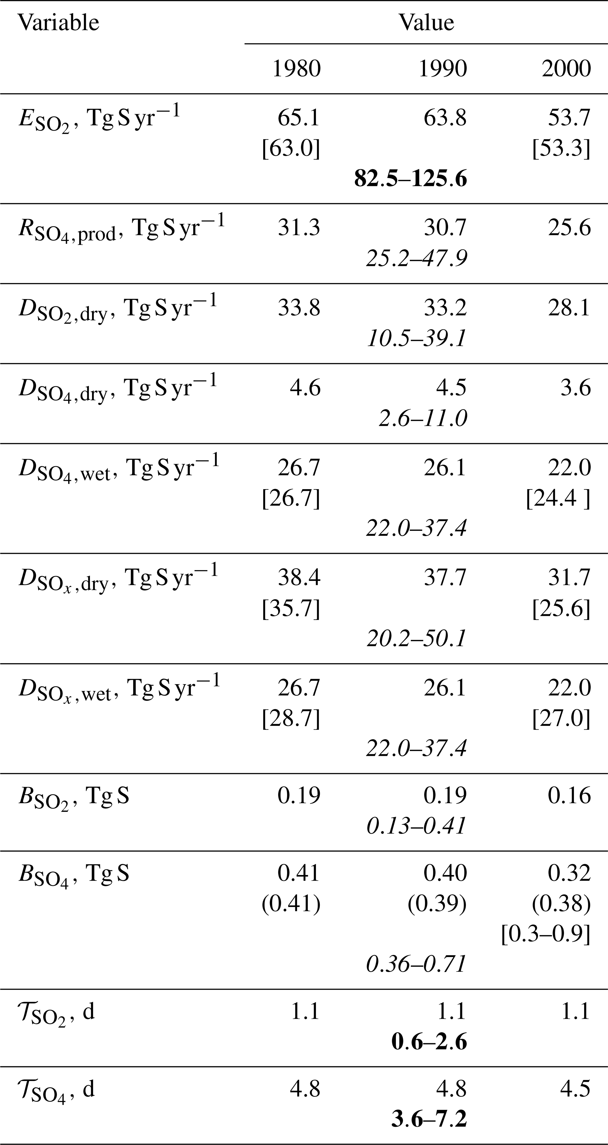
Table 2 Global sulfur budget in year 1990 as simulated by ChAP in comparison to other available estimates. The ACCMIP estimates are in square brackets and are either from Myhre et al. (2013) (their Table 4, sulfate burden) or Lamarque et al. (2013a) (emission and depositions). The values in parentheses are from the CMIP5 database (https://tntcat.iiasa.ac.at/RcpDb/, last access: 1 December 2020). Estimates in quotes are from Table 5.5 of IPCC TAR (Houghton et al., 2001) ascribed to year 1990. Bold font shows the values as they are reported in this table, and italic font is for the quantities which are rescaled by the ratio of our emissions in 1990 and the mean IPCC TAR ($\mathrm{0.65}=\mathrm{63.8}/\mathrm{98.2}$).

In addition, we use two datasets based on the assimilation of the available measurements into the chemical transport models: the Copernicus Atmosphere Monitoring Service (CAMS) (Inness et al., 2019) and the Meteorological Synthesizing Centre–West of the European Monitoring and Evaluation Programme (EMEP MSC-W) (Simpson et al., 2012); see Figs. S4–S7. These data cannot be used for direct comparison to our simulations because they are forced by both anthropogenic and natural emissions into the atmosphere, and the impact of the latter emissions can not be factored out because no pre-industrial simulations are available. However, we can compare our simulations with both datasets in the regions of strong anthropogenic sulfate pollution of the atmosphere, such as Europe, South-East Asia or North America (Chin et al., 2000) assuming that the anthropogenic sulfur load dominates over the natural one. Similar intercomparison may be made with individual model simulations summarised in Table 5.5 of IPCC TAR (Houghton et al., 2001). We note that, in contrast to the CMIP5 and ACCMIP datasets, CAMS and EMEP MSC-W were prepared by using meteorology that changes from year to year, making makes such comparison less straightforward. The individual model simulations in the IPCC TAR Table 5.5 were performed in a stationary fashion, with the year-to-year changes in meteorology only due to internal model variability. Therefore, we can consider them as also being run with “almost constant” meteorological fields, which makes our comparison with these simulations more straightforward.

Below we first discuss the performance of our scheme with respect to simulation of SO₂, because it is independent of the SO₄ performance. Then we proceed with a similar discussion of SO₄ simulation, which in contrast depends on the calculated SO₂ burden. We note that the maximum anthropogenic SO₂ emissions into the atmosphere in the CMIP5 data correspond to the 1980 time slice. However, because the model results for 1990 are quite similar to those for 1980 and because the most data are available staring from the year 2000, we use the time slice for 1990 as a primary model output to compare to the existing data. In such cases, we use the year 2000 time slice as a primary source for comparison.

5.1 Simulation of SO₂ burden and near-surface concentration

At the global scale, about half of the SO₂ emissions in our model are consumed by the chemical SO₄ production in the atmosphere, and the other half is deposited to the surface in the form of sulfur dioxide (Table 2). These fractions are within the ranges reported in IPCC TAR Table 5.5 (SO₂ deposition is from 18 % to 56 % of the prescribed emission rate with ensemble mean and ensemble standard deviations 42±12 %; SO₄ production is correspondingly from 42 % to 74 %, 57±12 %). Anthropogenic sulfur dioxide burden monotonically increases until 1980, reaches ≈0.2 Tg S in 1970–1990, and drops to 0.16 Tg S in 2000 (Table 2, Fig. 3a). These burdens are in the lower range of the values derived from IPCC TAR Table 5.5 (Table 2). The sulfur dioxide lifetime in the atmosphere in the model is close to 1.1 d. This value is within the respective lifetimes reported in IPCC TAR Table 5.5. This lifetime in our simulations changes non-systematically between different time slices with a standard deviation of 0.02 d. Such variations are caused by the employed smoothing procedure.

Figure 3 The globally and annually averaged modelled SO₂ mass in the atmosphere (a) and the respective annual mean (b, c), December–February mean (d, e), and June–August mean (f, g) burdens per unit area in 1990 (b, d, f) and 2000 (c, e, g). The green box shows the respective emission-rescaled IPCC TAR Table 5.5 estimate (see the caption of Table 2) and its median.

For the 1990 and 2000 time slices, annual mean sulfur dioxide burden exhibits maxima in the regions of the strong anthropogenic pollution – Europe, South-East Asia, and eastern North America, where $B_{{\mathrm{SO}}_{\mathrm{2}}}$ is typically larger than 2 mg S m⁻² and in some grid cells is in excess of 5 mg S m⁻² (Fig. 3b–e). Smaller maxima of $B_{{\mathrm{SO}}_{\mathrm{2}}}$ with typical values 1–2 mg S m⁻² are found in southern Africa and in the western part of South America. In 1990 (as well as in previous years) SO₂ in Europe is larger than in South-East Asia, while in 2000 the regional maximum in South-East Asia is larger than in other regions. This is quite expected based on the regional differences in sulfur dioxide emissions (Fig. S3; the emissions in years 1980 and 1990 are similar to each other).

Figure 4 The modelled near-surface concentration of sulfur dioxide in 1990 (a, c, e) and 2000 (b, d, f). The top, middle, and bottom rows show annual means, the average for boreal winter, and the average for boreal summer, respectively.

Geographical distribution of near-surface SO₂ concentration basically follows that of the sulfur dioxide total column burden (Fig. 4). Again, in the anthropogenically polluted regions $q_{{\mathrm{SO}}_{\mathrm{2}},\mathrm{s}}$ in the last decades of the 20th century is above 2 µg S m⁻³, and in Europe it is larger than 5 µg S m⁻³ until the 1990 time slice. In the southern Africa and western South America source regions, near-surface SO₂ concentration is from 1 to 2 µg S m⁻³.

The time slice for year 2000 in the model reasonably agrees with the CAMS data for 2003–2010 in the above-mentioned regions of strong pollution for both total column burden and near-surface concentration of sulfur dioxide (Figs. S4 and S5). Nonetheless, one notes some overestimation of both variables in Europe and some underestimate in South-East Asia. In Europe, the ChAP-simulated $q_{{\mathrm{SO}}_{\mathrm{2}},\mathrm{s}}$ also agrees with the EMEP MSC-W data for 2000–2005 (Fig. S6). The larger discrepancy in our simulations in Europe from the CAMS data than from the EMEP MSC-W data is at least partly explained by difference in covered period between the CAMS and EMEP MSC-W datasets. Namely, provided that aerosol emissions in Europe continuously decrease in the early 21st century, one may expect that the mean over 2000–2006 is closer to the time slice 2000 compared to the 2003–2020 average. We also note that the ChAP-simulated values in central Europe in 1990 generally agree with the older EMEP data for the mid-1990s as summarised by Semenov et al. (1998). Moreover, in the regions of strong pollution, our burden for the year 1990 is similar to that simulated with the NCAR CCM (Barth et al., 2000), GISS (Chin et al., 2000), and CCCMA (Lohmann et al., 1999) models. Near-surface sulfur dioxide concentrations are comparable to those simulated with the IMAGES (Pham et al., 1995) and GISS (Chin et al., 1996) models.

5.2 Simulation of SO₄ burden and near-surface concentration

Similar to the trend for SO₂, the total column burden of anthropogenic sulfates increases monotonically until 1980, reaches ≈0.4 Tg S in 1970–1990, and drops to 0.32 Tg S in 2000 (Table 2, Fig. 5a). These values are only slightly smaller than the corresponding values from the CMIP5 database. In addition, the value for time slice 2000 is close the range obtained in the respective ACCMIP exercise (Myhre et al., 2013), although they are in the lower part of this range. Our simulated total column burden of sulfates in the year 1990 is also within the IPCC TAR estimates, albeit again in its lower part.

Figure 5 The globally and annually averaged modelled SO₄ mass in the atmosphere (a) and annual mean burdens per unit area (b–e) in the model (b, d) and in the CMIP5 database (c, e) in the years 1990 (b, c) and 2000 (d, e). In (a), horizontal lines on the colour boxes depict corresponding medians. The ACCMIP data are taken from Myhre et al. (2013, their Table 4). The IPCC TAR data are adopted from their Table 5.5 and are emission-rescaled (see the caption of Table 2).

Similar to what it was for sulfur dioxide, sulfate lifetime in the atmosphere in the model changes non-systematically between different time slices with a mean of 4.8 d and standard deviation of 0.2 d. Again, these variations are caused by the employed smoothing procedure. The value of ${\mathcal{T}}_{{\mathrm{SO}}_{\mathrm{4}}}$ for the year 1990 time slice is within the respective lifetimes reported in individual model simulations (Houghton et al., 2001, Table 5.5). In addition, the modelled ${\mathcal{T}}_{{\mathrm{SO}}_{\mathrm{4}}}$ is in agreement with the recent AeroCom phase III simulations for the year 2100, which leads to a range from 2.6 to 7.0 d with an ensemble mean of 4.9 d and ensemble standard deviation of 1.6 d (Gliß et al., 2021).

As expected, the principal regions of atmospheric pollution by sulfates are similar to those obtained for sulfur dioxide in the previous section. However, because of several-fold larger ${\mathcal{T}}_{{\mathrm{SO}}_{\mathrm{4}}}$ relative to ${\mathcal{T}}_{{\mathrm{SO}}_{\mathrm{2}}}$, sulfates are transported at larger distances in comparison to sulfur dioxide, and the individual source regions become visually connected on maps. In Europe, South-East Asia, and in south-eastern North America, $B_{{\mathrm{SO}}_{\mathrm{4}}}$ from the 1970s till the end of the simulation is in excess of 2 mg S m⁻², and it is above 5 mg S m⁻² for large areas in Europe and in South-East Asia during the period of the strongest SO₄ anthropogenic loading – in 1980 and in 1990 (Figs. 5–7). In the smaller in magnitude spatial maximum in southern Africa, in 1970–2000 this variable typically amounts 1–2 mg S m⁻². This is somewhat in contrast to another spatial maximum in South America – despite the fact that sulfur dioxide burdens per unit area in South America and in southern Africa are similar in 1970–2000 in our simulations, the respective SO₄ burden in South America is closer to the European, South-East Asian, and North American ones than to that in southern Africa. This difference is caused by very small zonal velocity in the South American source region (Fig. S2), which leads to very small transport of sulfates out of this region. In turn, the effect of horizontal transport is less pronounced for sulfur dioxide owing to the difference between ${\mathcal{T}}_{{\mathrm{SO}}_{\mathrm{4}}}$ and ${\mathcal{T}}_{{\mathrm{SO}}_{\mathrm{2}}}$.

Figure 6 December–February mean sulfate burdens per unit area in the model (a, c) and in the CMIP5 database (b, d) in the years 1990 (a, b) and 2000 (c, d).

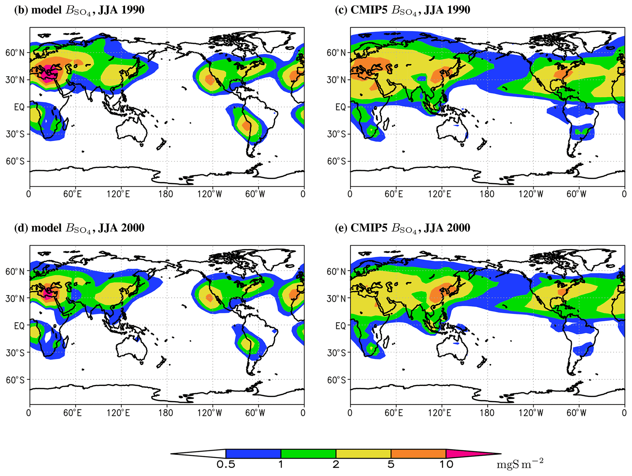
Figure 7 Similar to Fig. 6 but for means over June–August.

Geographic distribution of the modelled $B_{{\mathrm{SO}}_{\mathrm{4}}}$ as a whole is similar to that in the CMIP5 database (Figs. 5–7). However, for the period of the strongest SO₂ atmospheric emissions, the burden of sulfates in Europe is systematically overestimated by our model, especially in winter (Figs. 6 and 7). For summer, the correspondence between the ChAP-simulated and CMIP5 burdens is better. The agreement of SO₄ burden per unit area in South-East Asia depends on season: in winter our model overestimates the sulfates burden in this region and in summer it underestimates it but to a lesser extent than in winter. Mutual compensation between the model biases in different seasons led to overall reasonable simulation of sulfate burden per unit area in this source region. The magnitude of $B_{{\mathrm{SO}}_{\mathrm{4}}}$ in the North American source regions is basically correct, but during summer the maximum in this region is shifted to the west. The latter feature is not exhibited in winter. The $B_{{\mathrm{SO}}_{\mathrm{4}}}$ magnitudes in the source regions in the Southern Hemisphere are overestimated for the whole year.

Compared to the CAMS reanalysis (Fig. S4) in major source regions, our model overestimates sulfate burden per unit area in Europe with the larger discrepancy in winter then in summer. The $B_{{\mathrm{SO}}_{\mathrm{4}}}$ pattern in the South-East Asian source region is underestimated – this differs from that obtained in the comparison between our ChAP simulation and the CMIP5 database. The latter difference is at least partly due to difference in covering periods (recall that CAMS is for 2003–2010). Again, the magnitude of the SO₄ burden in the North American source region is realistic in ChAP, but now we see that even the location of maximum is correct. Thus, our previous conclusion about this location points to some possible shortcomings in the CMIP5 dataset. In the Southern Hemisphere, our model overestimates sulfate burdens per unit area in both the southern African and South American source regions. In addition, $B_{{\mathrm{SO}}_{\mathrm{4}}}$ in the Northern Hemisphere source regions is similar to those reported in the simulations with the NCAR CCM (Barth et al., 2000; Rasch et al., 2000), ECHAM (Feichter et al., 1996; Roelofs et al., 1998), GISS (Chin et al., 2000), and CCCMA (Lohmann et al., 1999) models.

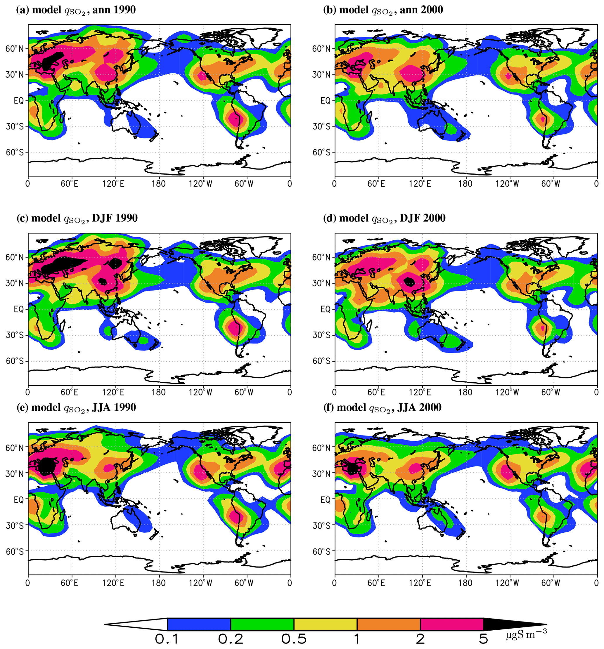
Figure 8 Similar to Fig. 4 but for the near-surface $q_{{\mathrm{SO}}_{\mathrm{4}}}$ concentration.

Geographic distribution of near-surface SO₄ concentration, $q_{{\mathrm{SO}}_{\mathrm{4}},\mathrm{s}}$, follows the corresponding distribution of $B_{{\mathrm{SO}}_{\mathrm{4}}}$ (Fig. 8). Identically to sulfur dioxide, this is a direct consequence of Eq. (2). In the anthropogenically polluted regions, $q_{{\mathrm{SO}}_{\mathrm{4}},\mathrm{s}}$ in the last decades of the 20th century is above 2 µg S m⁻³, and in Europe during summer 1990 it is larger than 5 µg S m⁻³. In southern Africa and in western South America, near-surface SO₂ concentration is typically above 0.5 µg S m⁻³. The simulated near-surface SO₄ concentrations are generally similar to those of the IMAGES (Pham et al., 1995) and GISS (Chin et al., 1996) models.

The modelled $q_{{\mathrm{SO}}_{\mathrm{4}},\mathrm{s}}$ in year 2000 in the principal source regions reasonably corresponds to the CAMS data for 2003–2010 (Fig. S5) but with an overestimate in Europe in summer and an underestimate in South-East Asia throughout the year. In Europe, our time slice for the year 2000 systematically exhibits a larger near-surface concentration of sulfates relative to the EMEP MSC-W data for 2000–2005 (Fig. S6).

5.3 Simulation of annual SO_x deposition

Owing to the mass conservation, the global SO_x deposition in the model is equal to the applied sulfur dioxide emissions. Depending on time slice, dry SO_x deposition $D_{{\mathrm{SO}}_x,\text{dry}}=D_{{\mathrm{SO}}_{\mathrm{2}},\text{dry}}+D_{{\mathrm{SO}}_{\mathrm{4}},\text{dry}}$ explains from 55 % to 59 % of the total SO_x deposition (mostly in the form of SO₂), and wet deposition $D_{{\mathrm{SO}}_x,\text{wet}}=D_{{\mathrm{SO}}_{\mathrm{4}},\text{wet}}$ explains another 41 %–45 % (only in the SO₄ form by design) (Table 2, Fig. 9a). The contribution of wet SO_x deposition in 1980 and 2000 is also similar to that obtained from ACCMIP (46 % and 51 %, respectively, Lamarque et al., 2013a) and is within the ranges reported in Table 5.5 of Houghton et al. (2001) for year 1990 (from 37 % to 64 %, with mean of 47 % and median of 45 %).

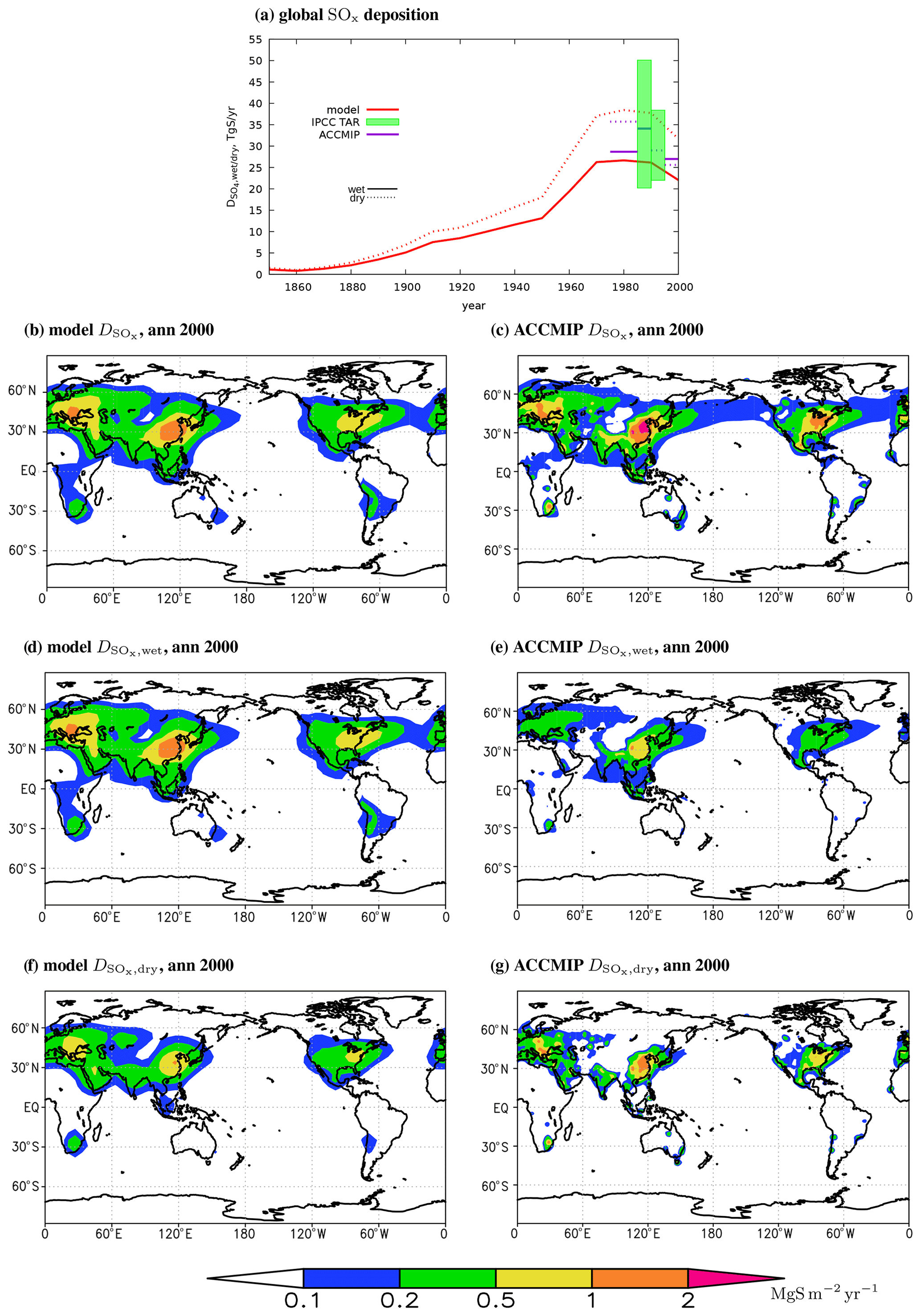
Figure 9 Global SO_x deposition (a) and total (b, c), wet (d, e), and dry (f, g) SO_x depositions per unit area in the model (b, d, f) and in the ACCMIP phase II simulations (c, e, g) for the year 2000. In (a), horizontal lines on the colour boxes depict corresponding medians. The ACCMIP data are taken from Lamarque et al. (2013a). The IPCC TAR data are adopted from their Table 5.5 and are emission-rescaled (see text); their dry and wet contributions are plotted at different 5-year intervals near the year 1990 for visual purposes.

Geographic distribution of the total SO_x deposition $D_{{\mathrm{SO}}_x}=D_{{\mathrm{SO}}_x,\text{wet}}+D_{{\mathrm{SO}}_x,\text{dry}}$ is very close to the sulfur dioxide emissions in a given year (cf. Fig. 9a with Fig. S3d and Fig. S7a with Fig. S3e). For year 2000, total deposition is above $\mathrm{1}\mathrm{Mg}\mathrm{S}{\mathrm{m}}^{-\mathrm{2}}{\mathrm{yr}}^{-\mathrm{1}}$ in the cores of the Northern Hemisphere source region and is above $\mathrm{0.2}\mathrm{Mg}\mathrm{S}{\mathrm{m}}^{-\mathrm{2}}{\mathrm{yr}}^{-\mathrm{1}}$ in the respective Southern Hemisphere source cores (Fig. 9a). In the year 1980 (and in 1990 as well; not shown) the corresponding values in Europe are even larger, $>\mathrm{2}\mathrm{Mg}\mathrm{S}{\mathrm{m}}^{-\mathrm{2}}{\mathrm{yr}}^{-\mathrm{1}}$. For both years there is a quite close agreement between the modelled $D_{{\mathrm{SO}}_x}$ and the ACCMIP data (Figs. 9b and c and S7a and b). Again, this is a validation for our numerics and for our code rather than for the implemented physics because total SO_x deposition near any source region is controlled by prescribed emissions and by prescribed winds.

A more stringent test of the implemented physics is a subdivision of total SO_x deposition into wet and dry deposition (Figs. 9d–g and S7c–f). This shows that ChAP generally overestimates wet deposition and underestimates dry deposition relative to the ACCMIP simulations. This is not visible in the global numbers (Table 2, Fig. 9a) because of differences in extent of the regions in which “substantial” (say, $\ge \mathrm{0.1}\mathrm{Mg}\mathrm{S}{\mathrm{m}}^{-\mathrm{2}}{\mathrm{yr}}^{-\mathrm{1}}$ in Figs. 9d–g and S7c–f) deposition occurs. However, in Europe an agreement is markedly better with the EMEP MSC-W data (Fig. S8). The ChAP-simulated wet SO_x deposition in the year 1990 (which is rather similar to the year 1980) is also in a general agreement with the simulations with the MOGUNTIA (Langner and Rodhe, 1991), IMAGES (Pham et al., 1995), and GISS (Koch et al., 1999) models.

6 Limitations of the current version of the scheme and future prospects

It was demonstrated in the previous section that, despite its apparent simplicity, ChAP 1.0 is able to reproduce gross characteristics of the tropospheric sulfur cycle for late 19th century and the whole 20th century. However, our model has inherent limitations, which have to be discussed together with figuring out the way to extend and improve ChAP.

First of all, in the contemporary version of ChAP does not implement any scheme for contribution of dimethyl sulfide (DMS) and other minor atmospheric sulfur species to chemical production sulfur dioxide. DMS emissions are basically biogenic and mostly limited to the ocean. According to the existing estimates, atmospheric DMS burden changes by no more than a few percent even under strong climate changes, as assessed in Houghton et al. (2001, Sect. 5.5.2.1) and further reported by Bopp et al. (2003) and by Kloster et al. (2007). Thus, given the present-day DMS source strength up to 28 Tg S yr⁻¹ (Lana et al., 2011; Galí et al., 2018; Wang et al., 2020), DMS lifetime in the atmosphere from 1 to 3 d, and its complete conversion to SO₂ (Table 2 in Koch et al., 1999), such an increase would change sulfur dioxide and sulfate burdens in the troposphere mostly over oceans. We plan to implement this source into our scheme in future. ChAP also misses other natural sulfur sources into the atmosphere: non-eruptive volcanic sources have a present-day strength of 23±2 Tg S yr⁻¹; SO₂ release from volcanic eruptions is an order of magnitude smaller and is partly loaded into the stratosphere rather than into the troposphere (Carn et al., 2017) and from biomass burning (correspondingly, $\approx \mathrm{1.2}\mathrm{Tg}\mathrm{S}{\mathrm{yr}}^{-\mathrm{1}}$ (van der Werf et al., 2017); this source is partly anthropogenic). However, the non-eruptive volcanic source may be considered constant in time. The biomass burning source, even if its strength triples following other wildfire emissions (which may occur under a high-CO₂ anthropogenic scenario; Eliseev et al., 2014), would not change the global sulfur budget markedly but may be important at a regional level. These sources may be readily added to our scheme as contributions to $E_{{\mathrm{SO}}_{\mathrm{2}}}$. We plan to implement them in the future provided that a hosting EMIC is able to simulate natural fires (Sitch et al., 2005; Eliseev and Mokhov, 2011; Eliseev, 2011; Eliseev et al., 2014, 2017).

The model knows nothing about the availability of oxidants (OH, HO₂, and O₃). This is apparently equivalent to the assumption that these oxidants are always abundant. Partly this assumption is ameliorated by relating the atmospheric sulfur dioxide oxidation rate to cloud fraction, which is a characteristic of the atmospheric hydrological cycle. Nevertheless, a hint that this assumption should be relaxed may be obtained from mutual comparison of global burdens of SO₂ and SO₄: while both are in the lower half of the IPCC TAR range, the former is closer to the corresponding median (Fig. 3a) in comparison to the latter (Fig. 5a). It may be possible to implement stationary equations for hydroxyl- and peroxide-radicals owing to their very short lifetimes (no more than few seconds in the lower troposphere; Lelieveld et al., 2016). However, such a stationary assumption is likely to be problematic for ozone with its typical lifetime of several weeks (Young et al., 2013). One more option would be just to prescribe the latitudinal dependence of the chemical conversion rate on latitude assuming that this dependence reflects the corresponding dependence of the OH abundance (see, e.g. Rémy et al., 2019, their Eq. 16).

Our horizontal transport solver is very simplistic and is able to provide more or less realistic results only for species with lifetimes up to few days (Sect. 2.1 and 2.2). Taking into account the estimated horizontal advection length scales, $L_{{\mathrm{SO}}_{\mathrm{2}}}$ and $L_{{\mathrm{SO}}_{\mathrm{4}}}$, one sees that our approach is well justified for zonal advection (because a large number of grid cells is typically included into a zonal loop in Sect. 2.2) but becomes more suspicious for the meridional advection. This shortcoming, however, is somewhat compensated by our rather large value of n_smo, which at mid-latitudes corresponds to the length scale of $(\mathrm{1}-\mathrm{2})\times {\mathrm{10}}^{\mathrm{3}}\mathrm{km}$ – this is pretty comparable to $L_{{\mathrm{SO}}_{\mathrm{4}}}$. In future we plan to either improve our solver or just to combine cells in meridional direction to make transporting species possible over longer distances owing to decreased meridional resolution.

Another transport-solver-related issue is due to implemented smoothing procedure. This implementation is reasoned by neglect of synoptic scales in our transport routine – we use only monthly mean winds. While ChAP is formally linear with respect to horizontal winds (Eq. 5) and therefore allows averaging over synoptic-scale motions, possible time correlations between synoptic-scale variations of winds and pollutant burdens make the underlying processes non-linear (Saltzman, 1978; Branscome, 1983; Petoukhov et al., 2008; Coumou et al., 2011). Further, one may argue that the corresponding mixing length (thus, n_smo) could be made dependent on synoptic-scale kinetic energy (Branscome, 1983; Coumou et al., 2011). At the time of writing, n_smo is a parameter of the scheme, but in future it could become dependent on large-scale atmospheric state (e.g. on the state with timescales and space scales larger than synoptic ones).

In our scheme we neglected wet deposition of sulfur dioxide. This was done based on the synthesis of simulations listed in Table 5.5 of IPCC TAR (Houghton et al., 2001), in which wet deposition of SO₂ explained no more than 15 % of the sulfur dioxide budget. Only in CCM1-GRANTOUR (Chuang et al., 1997) and in the earlier version of GOCART (Chin et al., 1996) is this contribution from 15 % to 20 %. While the upper-end values from these papers are not negligible, $D_{{\mathrm{SO}}_{\mathrm{2}},\text{wet}}$ is still neglected. Its implementation would probably improve regional performance of our scheme. We acknowledge the neglect of $D_{{\mathrm{SO}}_{\mathrm{2}},\text{wet}}$ as a limitation of our scheme.

In addition, it is necessary to highlight that dry deposition of sulfates is still included in our scheme, despite its contribution to the SO₄ budget also being not as important relative to the SO₂ wet deposition at the global scale. For instance, for the IPCC TAR ensemble this contribution is ≤25 %. The reason for keeping $D_{{\mathrm{SO}}_{\mathrm{4}},\text{wet}}$ is mostly numeric: such a background deposition avoids a division by zero in regions with very small precipitation rate.

Gas-phase oxidation of sulfur dioxide is also formally neglected in the current version of ChAP. Depending on the model, the gas phase may or may not be an important process in converting SO₂ to SO₄ (see, e.g. Table 2 in Koch et al., 1999). However, our scheme still accounts implicitly for gas-phase oxidation of sulfur dioxide because the total sulfate production is optimised rather than only the in-cloud part. The reason for the latter is due to the major gas-phase oxidant (hydroxyl radical), which is also produced in the atmospheric hydrological cycle-related pathways. We neglect the sulfur dioxide oxidation by ozone as well. This unlikely to be covered by any tuning of Eq. (14), and we acknowledge it as a limitation for ChAP.

ChAP improvements may be achieved via more detailed formulations of wet deposition rates. Contemporary implemented formulation (Eq. 15) does not distinguish between different precipitation types: light rain, heavy rain, and snow. Light and heavy rains show principally different efficiencies for removing hygroscopic aerosols from the atmosphere (Allen et al., 2016; Wang et al., 2021). This is basically due to the difference in time exposures of aerosol for solutions of aerosol in droplets between these two kinds of precipitation. A similar effect also leads to the very low efficiency of snow as an aerosol remover. The work to implement a distinction between different precipitation types in our scheme is under way and is expected to be implemented into the next version of ChAP.

In a similar way, dry deposition rates may be prescribed to depend on land surface type. Typically, a distinction between the open ocean, snow and ice, and land without ice and snow is used in the models (e.g. Langner and Rodhe, 1991; Pham et al., 1995; Feichter et al., 1996; Roelofs et al., 1998; Rasch et al., 2000; Lohmann et al., 1999; Chin et al., 2000; Rémy et al., 2019). This possibility is omitted on purpose in this paper. The reasoning behind this choice is due to (i) the neglect of sulfur sources from the ocean to the atmosphere (which directly hampers tuning of $k_{{\mathrm{SO}}_{\mathrm{2}},\text{dry}}$ and $k_{{\mathrm{SO}}_{\mathrm{4}},\text{dry}}$ over the ocean) and (ii) as an attempt to demonstrate the ability of the present, simplistic version of ChAP to reproduce large-scale properties of the sulfur compounds distribution in the atmosphere. Nonetheless, we opt to try this option in future.

One more way of improving the calculation of near-surface concentrations of sulfur species is to account for regional differences of $H_{{\mathrm{SO}}_{\mathrm{2}}}$ and $H_{{\mathrm{SO}}_{\mathrm{4}}}$. For instance, large geographical, seasonal, and diurnal variations for vertical scale of different (but all similarly trapped in the planetary boundary layer) species in the atmosphere are observed (Jaenicke, 1993; Warneck, 2000). We plan to relate $H_{{\mathrm{SO}}_{\mathrm{2}}}$ and $H_{{\mathrm{SO}}_{\mathrm{4}}}$ to large-scale values of the planetary boundary layer depth (thus, to vertical mixing inside this layer). This work is currently underway at time of writing.

A more subtle issue is due to implementation of total cloud fraction in Eq. (14) for in-cloud oxidation rate. Because most sulfur conversion occurs in the lower half of the troposphere, one may argue that low cloud fraction would be a better predictor for this oxidation rate. We tried this option during development of ChAP and found no marked differences (apart somewhat different optimal values of parameters listed in Table 1). Thus, to be in line with the contemporary generation of EMICs, which mostly do not provide cloud fractions for different layers, we kept total cloud fraction as part of the input to our scheme instead of low cloud fraction.

The performance of the scheme was mainly tested against the CMIP5 data and the ACCMIP simulations. The basic reason for limiting validation to these datasets is due to our neglect of the natural sources of sulfur emissions into the atmosphere. This limitation is somewhat relaxed in the present paper by comparing it to the CAMS and EMEP output and to individual simulations in regions of strong anthropogenic pollution into the atmosphere. Our neglect of natural sulfur sources is also one of the reasons to exclude direct measurements of sulfur burdens (e.g. Aas et al., 2019). Another reason for this exclusion is due to possible complications owing to local features that are likely present in these direct, point-scale measurements. A meaningful use of such data would need to find their stratification into background and polluted stations and factor out such local-scale features, which is beyond the scope of the present study. Exclusion of such point-scale measurements is somewhat ameliorated by their assimilation into CAMS and EMEP. In addition, in future exercises we plan to replace the CMIP5 forcing with the CMIP6 one (Hoesly et al., 2018; Turnock et al., 2020).

A related issue is due to our use of the ERA cloud and precipitation fields rather than those based on direct measurements. For instance, arguably more reliable cloud fractions may be prescribed from the A-Train satellite observations (Minnis et al., 2011; Frey et al., 2008). Correspondingly, precipitation rate could be derived from the GPCP (Global Precipitation Climatology Project) data (an update from Huffman et al., 2009). Marked differences in the ERA-Interim fields from these data are documented, for instance, by Dolinar et al. (2016), Stengel et al. (2018), and Nogueira (2020). For instance, the underestimated rainfall rate in Europe in ERA-Interim (Nogueira, 2020) region may be the reason for our overestimate of $B_{{\mathrm{SO}}_{\mathrm{4}}}$ in this region, while the corresponding excessive precipitation rate in the Asian monsoon region could contribute to the underpredicted sulfate burden over South-East Asia. However, we prefer to keep the ERA-Interim cloud fractions and precipitation as forcing fields in our tuning exercise because they are at least dynamically consistent with other forcing fields.

Finally, choice of skill score is always subjective in tuning exercises like ours. We reported only one type of skill score (Eq. 16). However, we tried other skill scores as well, e.g. based on the root-mean-square error (RMSE) of simulations or by limiting the skill score calculations to the regions with sufficiently large SO₂ and SO₄ burdens. The first option (RMSE skill score) provided rather unrobust results. The second option did not result in a much improved simulation in comparison to that reported in Sect. 5. Therefore, we decided to use the skill score as outlined in Eq. (16).

7 Conclusions

A stationary, computationally efficient scheme for the sulfur cycle in the troposphere, ChAP 1.0 (Chemical and Aerosol Processes, version 1.0), is developed. This scheme is designed to be implemented into Earth system models of intermediate complexity (EMICs). The scheme accounts for sulfur dioxide emissions into the atmosphere, its deposition to the surface and oxidation to sulfates, and dry and wet deposition of sulfates on the surface. Horizontal transport of sulfur compounds in the atmosphere is tackled by representing model grid cells as non-interacting sources of particular sulfur species. The calculations with the scheme are forced by anthropogenic emissions of sulfur dioxide into the atmosphere for 1850–2000 adopted from the CMIP5 dataset and by the ERA-Interim meteorology. This setup assumes that natural sources of sulfur into the atmosphere remain unchanged during this period.

The ChAP output is compared to changes in the tropospheric sulfur cycle simulations: with the CMIP5 $B_{{\mathrm{SO}}_{\mathrm{4}}}$ data, with the IPCC TAR ensemble, and with the ACCMIP phase II simulations. In addition, in regions of strong anthropogenic sulfur pollution, ChAP results are compared to other data, such as the CAMS reanalysis, the EMEP MSC-W output, and individual model simulations. Our model reasonably reproduces characteristics of the tropospheric sulfur cycle known from these information sources. In particular, in 1980 and 1990, when the global anthropogenic emission of sulfur is at its maximum, global atmospheric burdens of SO₂ and SO₄ account for 0.2 and 0.4 Tg S, respectively. In our scheme, about half of the emitted sulfur dioxide is deposited to the surface, and the rest is oxidised into sulfates. In turn, sulfates are mostly removed from the atmosphere by wet deposition. The lifetime of the sulfur dioxide and sulfates in the atmosphere is close to 1 and 5 d, respectively. The differences between our simulations on one hand and the CAMS and EMEP MSC-W datasets on the other are partly (but likely far from completely) explained by the differences in time intervals covered by our simulations and by these datasets.

We highlight that, contrary to the previously available scheme for the tropospheric sulfur cycle designed for EMICs (Bauer et al., 2008), our scheme does not employ an assumption of fixed lifetimes for both SO₂ and SO₄. In ChAP, both lifetimes are determined by the conversion and deposition coefficients that depend on climate and on the burden of the compounds coming from the earlier steps of chemical chains.

We acknowledge the following major limitations of the contemporary version of ChAP:

• the omission of natural sulfur emissions and partial omission of some anthropogenic sulfur emissions into the troposphere,

• a neglect of SO₂ wet deposition and (partly) of its gas-phase oxidation,

• the very indirect relationship between the intensity of sulfur dioxide oxidation rate and the amount of major oxidants,

• the independent prescription of geography and climate state vertical scales for both sulfur species considered in the paper,

• the possibility that the approach is too simplistic to calculate chemical conversion rates and dry and wet depositions of sulfur compounds,

• the simplifications in the transport solver.

We plan to address these limitations during future development of our scheme.

Despite its simplicity, our scheme is able to reproduce gross characteristics of the tropospheric sulfur cycle during the historical period. Thus, it may be successfully used to simulate anthropogenic sulfur pollution in the atmosphere at coarse spatial scales and timescales. At the next stage, we are going to implement it into EMIC and reproduce direct radiative effect of sulfates on climate, their respective indirect (cloud- and precipitation-related) effects, and the impact of sulfur compounds on the terrestrial carbon cycle.