the Creative Commons Attribution 4.0 License.
the Creative Commons Attribution 4.0 License.
 | 21 Dec 2021
Non-Hydrostatic RegCM4 (RegCM4-NH): model description and case studies over multiple domains
Paolo Stocchi
Emanuela Pichelli
Jose Abraham Torres Alavez
Russell Glazer
Graziano Giuliani
Fabio Di Sante
Rita Nogherotto
Filippo Giorgi
We describe the development of a non-hydrostatic version of the regional climate model RegCM4, called RegCM4-NH, for use at convection-permitting resolutions. The non-hydrostatic dynamical core of the Mesoscale Model MM5 is introduced in the RegCM4, with some modifications to increase stability and applicability of the model to long-term climate simulations. Newly available explicit microphysics schemes are also described, and three case studies of intense convection events are carried out in order to illustrate the performance of the model. They are all run at a convection-permitting grid spacing of 3 km over domains in northern California, Texas and the Lake Victoria region, without the use of parameterized cumulus convection. A substantial improvement is found in several aspects of the simulations compared to corresponding coarser-resolution (12 km) runs completed with the hydrostatic version of the model employing parameterized convection. RegCM4-NH is currently being used in different projects for regional climate simulations at convection-permitting resolutions and is intended to be a resource for users of the RegCM modeling system.
- Article
(7299 KB) - Full-text XML
- BibTeX
- EndNote


Since the pioneering work of Dickinson et al. (1989) and Giorgi and Bates (1989), documenting the first regional climate modeling system (RegCM, version 1) in the literature, the dynamical downscaling technique based on limited-area regional climate models (RCMs) has been widely used worldwide, and a number of RCM systems have been developed (Giorgi, 2019). RegCM1 (Dickinson et al., 1989; Giorgi and Bates, 1989) was originally developed at the National Center for Atmospheric Research (NCAR) based on the Mesoscale Model version 4 (MM4) (Anthes et al., 1987). Then, further model versions followed: RegCM2 (Giorgi et al., 1993a, b), RegCM2.5, (Giorgi and Mearns, 1999), RegCM3 (Pal et al., 2007) and lastly RegCM4 (Giorgi et al., 2012). Except for the transition from RegCM1 to RegCM2, in which the model dynamical core was updated from that of the MM4 (Anthes et al., 1987) to that of the MM5 (Grell et al., 1994), these model evolutions were mostly based on additions of new and more advanced physics packages. RegCM4 is today used by a large community for numerous projects and applications, from process studies to paleo and future climate projections, including participation in the Coordinated Regional Downscaling EXperiment (CORDEX, Giorgi et al., 2009; Gutowski et al., 2016). The model can also be coupled with ocean, land, chemistry and aerosol modules in a fully interactive way (Sitz et al., 2017).
The dynamical core of the standard version of RegCM4 is hydrostatic, with σ(p) vertical coordinates. As a result, the model can be effectively run for grid spacings of ∼ 10 km or larger, for which the hydrostatic assumption is valid. However, the RCM community is rapidly moving to higher resolutions of a few kilometers, i.e., “convection-permitting” (Prein et al., 2015; Coppola et al., 2020), and therefore the dynamical core of RegCM4 has been upgraded to include a non-hydrostatic dynamics representation usable for very high-resolution applications. This upgrade, which we name RegCM4-NH, is essentially based on the implementation of the MM5 non-hydrostatic dynamical core within the RegCM4 framework, which has an entirely different set of sub-grid model physics compared to MM5.
RegCM4-NH is already being used in some international projects focusing on climate simulations at convection-permitting kilometer scales, namely the European Climate Prediction System (EUCP, Hewitt and Lowe, 2018) and the CORDEX Flagship Pilot Study dedicated to convection (CORDEX-FPSCONV, Coppola et al., 2020), and it is starting to be used more broadly by the RegCM modeling community.
For example, the recent papers by Ban et al. (2021) and Pichelli et al. (2021) document results of the first multi-model experiment of 10-year simulations at the convection-permitting scales over the so-called greater Alpine region. Two different simulations with RegCM4-NH for present-day conditions have contributed to the evaluation analysis of Ban et al. (2021). They were carried out at the International Centre for Theoretical Physics (ICTP) and the Croatian Meteorological and Hydrological Service (DHMZ) using two different physics configurations. The results show that RegCM4-NH largely improves the precipitation simulation as compared to available fine-scale observations when going from coarse to high resolution, in particular for higher-order statistics, such as precipitation extremes and hourly intensity. Pichelli et al. (2021) then analyze multi-model ensemble simulations driven by selected Coupled Model Intercomparison Project – Phase 5 (CMIP5) global circulation model (CMIP5 GCM) projections for the decades 1996–2005 and 2090–2099 under the RCP8.5 scenario. ICTP contributed to the experiment with simulations using RegCM4-NH driven by the MOCH-HadGEM GCM (r1i1p1) in a two-level nest configuration (respectively, at 12 and 3 km grid). The paper shows new insights into future changes, for example an enhancement of summer and autumn hourly rainfall intensification compared to coarser-resolution model experiments, as well as an increase in frequency and intensity of high-impact weather events.
In this paper we describe the structure of RegCM4-NH and provide some illustrative examples of its performance, so that model users can have a basic reference providing them with background information on the model. In the next section we first describe the new model dynamical core, while the illustrative applications are presented in Sect. 4. Section 5 finally provides some discussion of future developments planned for the RegCM system.
In the development of RegCM4-NH, the RegCM4 as described by Giorgi et al. (2012) was modified to include, the non-hydrostatic dynamical core (idynamic =2 namelist option as described in RegCM-4.7.1/Doc/README.namelist of the source code) of the mesoscale model MM5 (Grell et al., 1994). This dynamical core was selected because RegCM4 already has the same grid and variable structure as MM5 in its hydrostatic core, which substantially facilitated its implementation (Elguindi et al., 2017).
The model equations with a complete description of the Coriolis force and a top radiative boundary condition, along with the finite-differencing scheme, are given in Grell et al. (1994). Pressure, p, temperature, T, and density, ϱ, are first decomposed into a prescribed reference vertical profile plus a time-varying perturbation. The prognostic equations are then calculated using the pressure perturbation values. Compared to the original MM5 dynamical core, the following modifications were implemented in order to achieve increased stability for long-term climate simulations (Elguindi et al. (2017) document any modifications which follow the choice of the non-hydrostatic dynamical core through the namelist parameter idynamic =2; further available user-dependant options, and the corresponding section in the namelist, are explicitly indicated):
- i.
The reference state temperature profile is computed using a latitude dependent climatological temperature distribution and thus is a function of the specific domain coordinates (base_state_pressure, logp_lrate parameters in &referenceatm) (Elguindi et al., 2017). These two parameters were hard-coded in the original MM5, while for the RegCM they are user configurable.
- ii.
The lateral time-dependent boundary conditions (iboudy in &physicsparam) for each prognostic variable use the same exponential relaxation technique (iboudy =5) described in Giorgi et al. (1993b). The linear MM5 relaxation scheme is also kept as an option (iboudy =1).
- iii.
The advection term in the model equations, which in the MM5 code is implemented using a centered finite-difference approach, was changed to include a greater upstream weight factor as a function of the local Courant number (Elguindi et al., 2017). The maximum value of the weight factor is user configurable (uoffc in &dynparam). As detailed in the MM5 model description (Grell et al., 1994), the horizontal advection term for a scalar variable X contributes to the total tendency as
where the m is the projection mapping factor, and, with respect to Fig. 1, assuming that the computation is to be performed for the gold cross point G, the averages are performed in the points . For the and terms, the average value is computed using, respectively, the values in points AC, BD, CD, AB.
In RegCM4 for the term p∗X, the model computes a weighted average value of the field using the value in gold+cyan and gold+green cross points with weights increasing the relative contribution of the upstream point up as a function of the local Courant number:
where f1, f2 are defined as the local Courant number for the 1D advection equations multiplied for a control factor:
- iv.
The water species (cloud, ice, rain, snow) term uses the same advection scheme as the other variables (Elguindi et al., 2017) and not a complete upstream scheme as in the MM5 code (Grell et al., 1994).
- v.
A local flux limiter reduces the advection terms in order to remove unrealistic strong gradients and its limits are user configurable (in the &dynparam section the maximum gradient fraction for advection is as follows: temperature, t_extrema, specific humidity, q_rel_extrema, liquid cloud content, c_rel_extrema, and for tracers, t_rel_extrema). This was hardcoded in the MM5 code, and the limits were not user configurable.
- vi.
The diffusion stencil of the Laplace equation uses a nine-point approach as in LeVeque (2007), and a topography-dependent environmental diffusion coefficient is added to reduce spurious diffusion along pressure coordinate slopes (Elguindi et al., 2017) as in the hydrostatic version of the code (Giorgi et al., 1993b). The change in stencil does not affect the overall fourth-order precision of the model but reduces the computational stencil size, thus reducing the communication overhead.
- vii.
The top boundary radiative condition (ifupr =1 in &nonhydroparam) adopted in the semi-implicit vertical differencing scheme to reduce the reflection of energy waves uses coefficients on a 13×13 matrix which are re-computed every simulation day and not kept constant throughout the whole simulation as in the MM5 code. This allows the model to be run for longer simulation times while not being strongly tied to the initial atmospheric conditions.
- viii.
The dynamical control parameter β in the semi-implicit vertical differencing scheme (nhbet in &nonhydroparam) used for acoustic wave damping (Elguindi et al., 2017) is user configurable (Klemp and Dudhia, 2008), while it is hard-coded in the MM5.
- ix.
A Rayleigh damping (ifrayd =1 in &nonhydroparam) of the status variables towards the input GCM boundary conditions can be activated in the top layers (rayndamp configuring the number of top levels to apply) with a configurable relaxation time (rayalpha0, Klemp and Lilly, 1978; Durran and Klemp, 1983; this is consistent with what is implemented in the Weather Research Forecast (WRF) model).
- x.
The water species time filtering uses the Williams (2009) modified filter with α=0.53 instead of the Robert–Asselin (RA) filter used by all the other variables. The ν factor in the RA filter is user configurable (gnu1 and gnu2 in &dynparam). This reduces the damping introduced by the Robert–Asselin filter and the computational diffusion introduced by the horizontal advection scheme.

Figure 1Schematic representation showing the horizontal advection scheme staggering for a scalar variable. Circles are U, V points. Crosses (X) represent scalar variable points. Squares (identifying points a,b,c,d) are points where weighted averages are calculated for variables contributing to advection on point G.
With these modifications, the model basic equations, under a leap-frog integration scheme, are (Elguindi et al., 2017)
where
with the vertical sigma coordinate defined as
ps is the surface pressure and p0 is the reference pressure profile. The total pressure at each grid point is thus given as
with pt being the top model pressure assuming a fixed rigid lid.
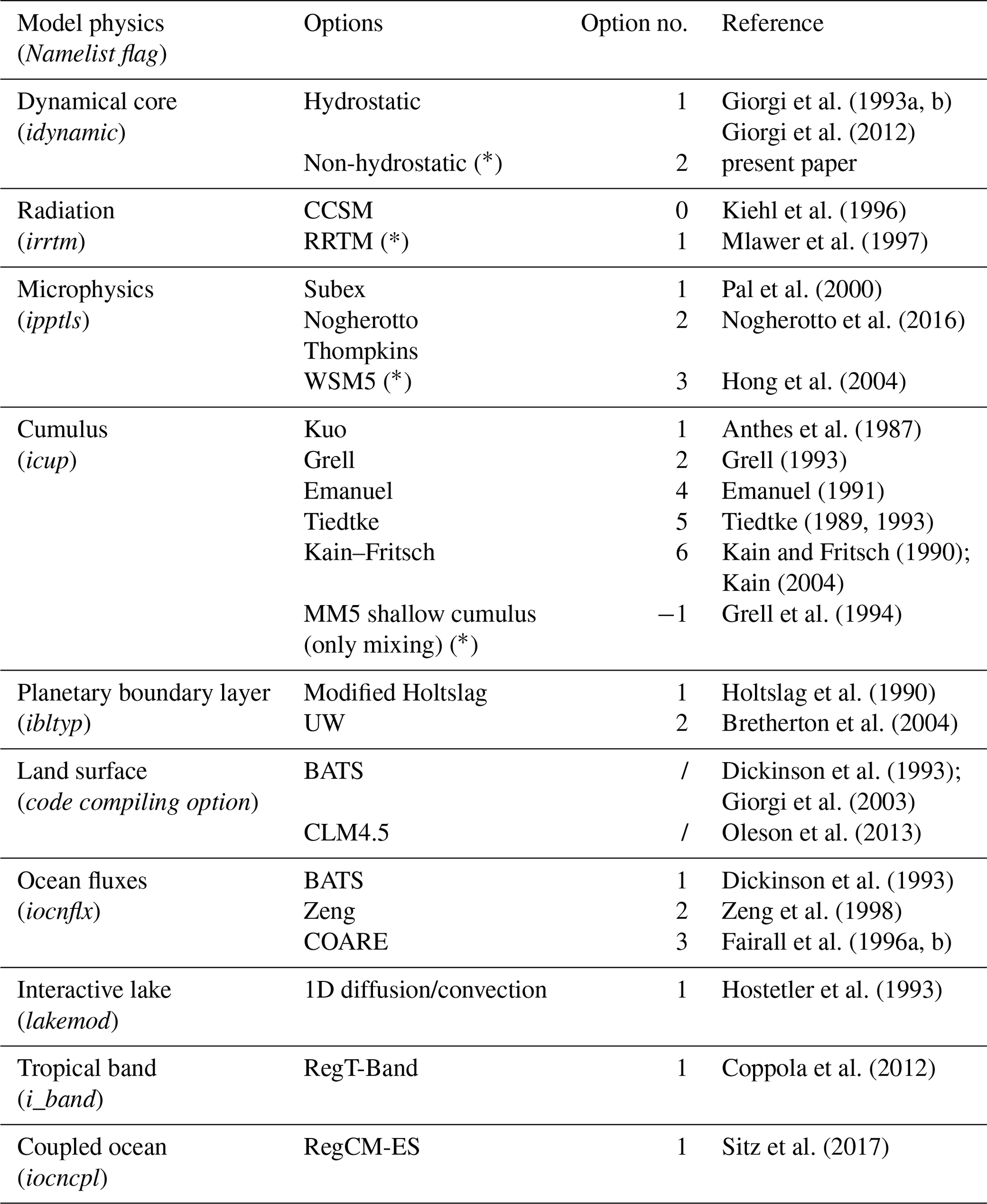
The model physics schemes for boundary layer, radiative transfer, land and ocean surface processes, cloud and precipitation processes are extensively described in Giorgi et al. (2012) and summarized in Table 1. For each physics component a number of parameterization options are available (Table 1) and can be selected using a switch selected by the user. As mentioned, the use of non-hydrostatic dynamics is especially important when going to convection-permitting resolutions of a few kilometers (Prein et al., 2015). At these resolutions the scale separation assumption underlying the use of cumulus convection schemes is not valid any more, and explicit cloud microphysics representations are necessary. The RegCM4 currently includes two newly implemented microphysics schemes, the Nogherotto–Tompkins (Nogherotto et al., 2016) and the WSM5 scheme from the Weather Research Forecast (WRF, Skamarock et al., 2008) model, which are briefly described in the next sections for information to model users.
Table 1Core and sub-grid physics scheme available in RegCM-NH. New schemes available with this release are starred (∗).
3.1 Nogherotto–Tompkins scheme
A new parameterization for explicit cloud microphysics and precipitation built upon the European Centre for Medium Weather Forecast's Integrated Forecast System (IFS) module (Tiedtke, 1993; Tompkins, 2007), was introduced in RegCM4 (ipptls =2 in µparam) by Nogherotto et al. (2016). In the present configuration, the scheme implicitly solves five prognostic equations for water vapor, qv, cloud liquid water, ql, rain, qr, cloud ice, qi, and snow, qs, but it is also easily extendable to a larger number of variables. Water vapor, cloud liquid water, rain, cloud ice and snow are all expressed in terms of the grid-mean mixing ratio. Cloud liquid and ice water content are independent, allowing the existence of supercooled liquid water and mixed-phase clouds. Rain and snow precipitate with a fixed terminal fall speed and can then be advected by the three-dimensional winds. A check for the conservation of enthalpy and of total moisture is ensured at the end of each time step. The governing equation for each variable is
The local variation in the mixing ratio qx of the variable x is given by the sum of Sx, containing the net sources and sinks of qx through microphysical processes (i.e., condensation, evaporation, auto-conversion, melting, etc.) and the sedimentation term, which is a function of the fall speed Vx. An upstream approach is employed to solve the equations. The source and sink contributors are divided into two groups according to the duration of the process they describe: processes that are considered to be fast relative to the model time step are treated implicitly while slow processes are treated explicitly. The processes taken into account (shown in Fig. 2) are the microphysical pathways across the five water variables: condensation, autoconversion, evaporation, cloud water collection (accretion) and autoconversion for warm clouds and freezing, melting, deposition and sublimation for cold clouds.
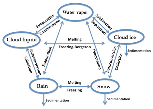
Figure 2Depiction of the new scheme, showing the five prognostic variables and how they are related to each other through microphysical processes.
For each microphysical pathway, phase changes are associated with the release or absorption of latent heat, which then impacts the temperature budget. The impact is calculated using the conservation of liquid water temperature TL defined as
Given that dTL=0, the rate of change in the temperature is given by the following equation:
where L(x) is the latent heat of fusion or evaporation, depending on the process considered, is the convective detrainment, and the third term in brackets is the sedimentation term.
At the end of each time step a check is carried out of the conservation of total water and moist static energy:
The scheme is tunable through parameters in the µparam section of the namelist (RegCM-4.7.1/Doc/README.namelist; Elguindi et al., 2017).
3.2 WSM5 scheme
RegCM4-NH also employs the Single-Moment five-class Microphysics Scheme of the WRF model (WSM5, Skamarock et al., 2008). This scheme (ipptls =3 in µparam) follows Hong et al. (2004) and, similarly to Nogherotto et al. (2016), includes vapor, rain, snow, cloud ice and cloud water hydrometeors. The scheme treats ice and water saturation processes separately, assuming water hydrometeors for temperatures above freezing and cloud ice and snow below the freezing level (Dudhia, 1989; Hong et al., 1998). It accounts for supercooled water and a gradual melting of snow below the melting layer (Hong et al., 2004; Hong and Lim, 2006). Therefore, the WSM5 and Nogherotto–Tompkins schemes have similar structures (Fig. 2) but also important differences.
Differently from the Nogherotto–Tompkins scheme, the WSM5 (as well as the other WSM schemes in WRF) prescribes an inverse exponential continuous distribution of particle size (for example, Marshall and Palmer (1948) for rain, Gunn and Marshall (1958) for snow). It also includes the size distribution of ice particles and, as a major novelty, the definition of the number of ice crystals based on ice mass content rather than temperature. Both the Nogherotto–Tompkins and WSM5 schemes include autoconversion, i.e., sub-time step processes of conversion of cloud water to rain and cloud ice to snow. For rain, Hong et al. (2004) use a Kessler (1969) type algorithm in WSM5 but with a stronger physical basis following Tripoli and Cotton (1980). The Nogherotto–Tompkins scheme also includes the original Kessler (1969) formula as an option but it makes available three other exponential approaches following Sundqvist et al. (1989), Beheng (1994), and Khairoutdinov and Kogan (2000). For ice autoconversion the Nogherotto–Tompkins scheme uses an exponential approach (Sundqvist, 1989) with a specific coefficient for ice particles (following Lin et al., 1983) depending on temperature, while the WSM5 uses a critical value of ice mixing ratio (depending on air density) and a maximum allowed ice crystal mass (following Rutledge and Hobbs, 1983) that suppresses the process at low temperatures because of the effect of air density. Finally, the WSM5 has no dependency on cloud cover for condensation processes, while the Nogherotto–Tompkins scheme uses cloud cover to regulate the condensation rate in the formation of stratiform clouds.
3.3 Illustrative case studies
Three case studies (Table 2) of heavy-precipitation events (HPEs) have been identified in order to test and illustrate the behavior of the non-hydrostatic core of the RegCM4-NH, with a focus on the explicit simulation of convection over different regions of the world. In two of the test cases, California and Lake Victoria, data from the ERA-Interim reanalysis (Dee et al., 2011) are used to provide initial and lateral meteorological boundary conditions (every 6 h) for an intermediate-resolution run (grid spacing of 12 km, with the use of convection parameterizations), which then provides driving boundary conditions for the convection-permitting experiments (Fig. 3). In the Texas case study, however, we nested the model directly in the ERA-Interim reanalysis given that such a configuration was able to accurately reproduce the HPE intensity. In this case the model uses a large lateral boundary conditions (LBCs) relaxation zone which allows the description of realistic fine-scale features driving this weather event (although not fully consistent with the Matte et al. (2017) criteria). All simulations start 24–48 h before the HPE (Table 2). The analysis focuses on the total accumulated precipitation over the entire model domain at 3 km resolution (Fig. 2) for the periods defined in Table 2. In the cases of California and Texas the evaluation also includes the time series of 6-hourly accumulated precipitation averaged over the region of maximum precipitation (black rectangles in Figs. 5a and 7a) because high temporal-resolution observations (NCEP/CPC) are also available (Table 3). The discussion of the case studies is presented in the next sections; the configuration files (namelists) with full settings for the three test cases are available at https://doi.org/10.5281/zenodo.5106399).
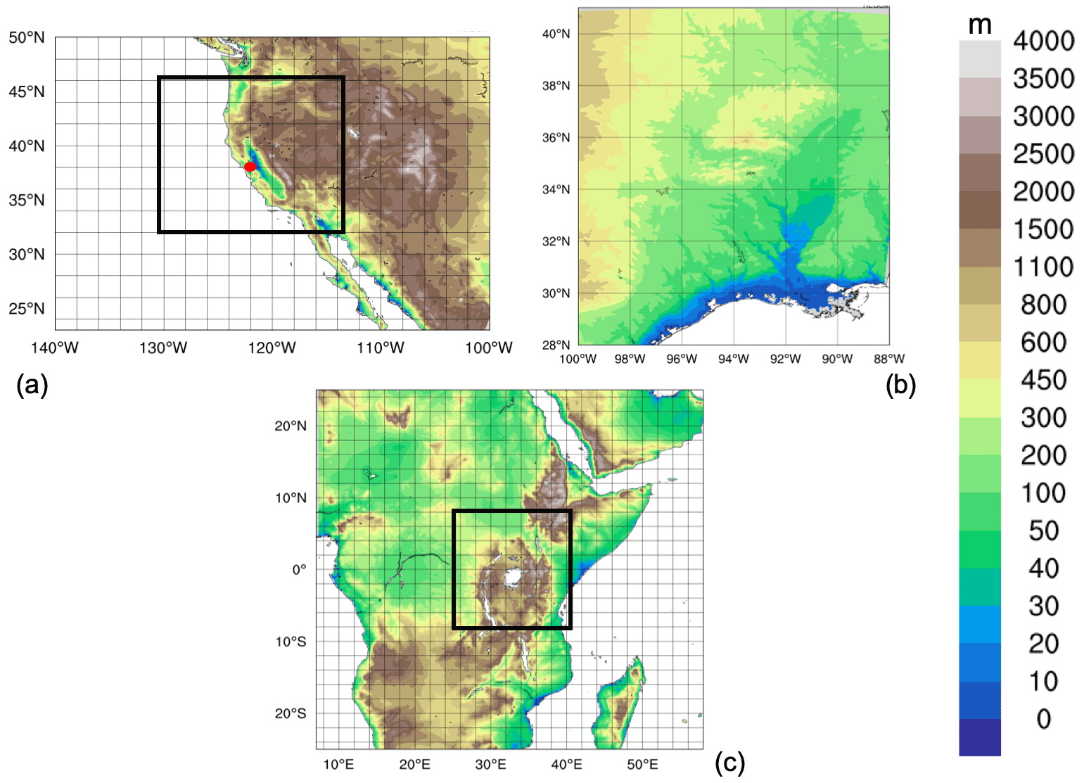
Figure 3Domains tested: (a) California (CAL), (b) Texas (TEX), (c) Lake Victoria (LKV). For CAL (a) and LKV (b) the black square shows the 3 km simulation domains nested in the 12 km domain in the figure. For the TEX case (b) the 3 km domain simulation is fed directly with the ERA-Interim reanalysis fields.
Table 2List of abbreviations and description of the test cases with corresponding 3 km domain sizes and simulation period.
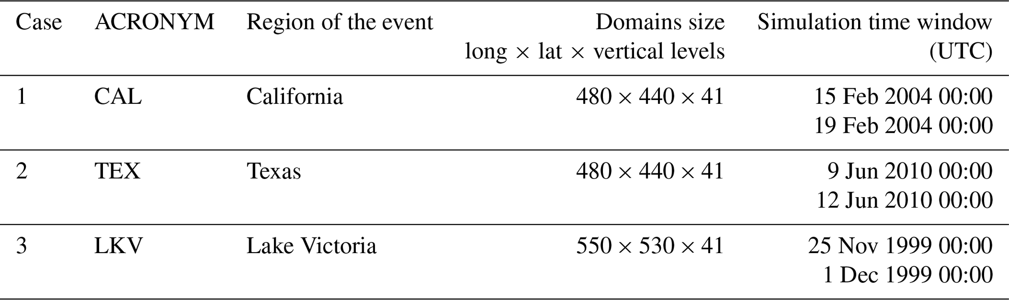
Table 3List of observed precipitation datasets used for comparison.
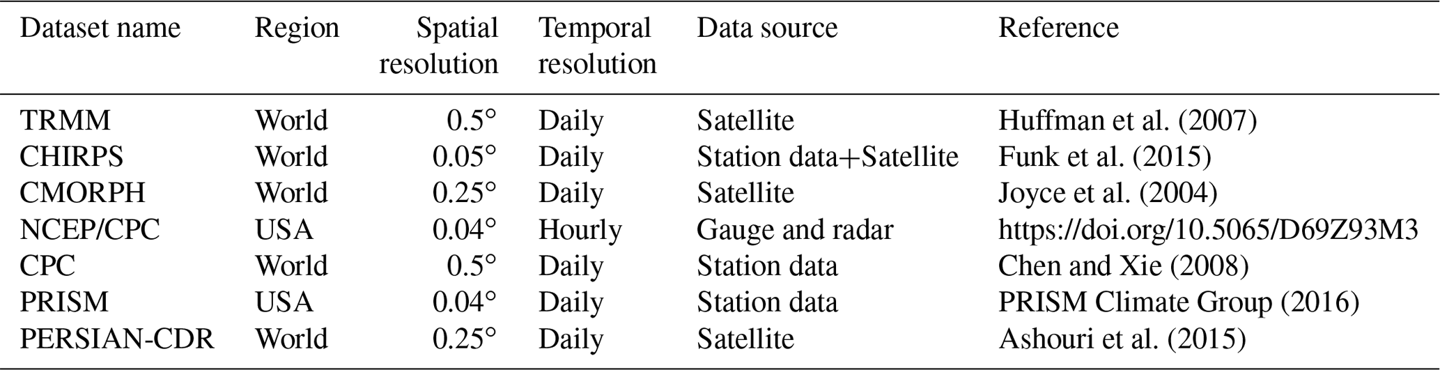
A key issue concerning the use of convection-permitting RCMs (CP-RCMs) is the availability of very high-resolution, high-quality observed datasets for the assessment and evaluation of the models, which is lacking for most of the world regions. Precipitation measurements come from essentially three distinct sources: in situ rain gauges, ground radar and satellite. In the present study we use seven observational datasets depending on the case study and the area covered, as described in Table 3. We have used Precipitation Estimation from Remotely Sensed Information using Artificial Neural Networks–Climate Data Record (PERSIAN-CDR), Climate Hazards Group InfraRed Precipitation with Station data (CHIRPS), the Climate Prediction Center morphing method (CMORPH), Tropical Rainfall Measuring Mission (TRMM), NCEP/CPC-Four Kilometer Precipitation Set Gauge and Radar (NCEP/CPC), CPC-Unified gauge-based daily precipitation estimates (CPC) and Parameter-elevation Regressions on Independent Slopes Model (PRISM) (Table 3). NCEP/CPC is a precipitation analysis which merges a rain gauge dataset with radar estimates. CMORPH and PERSIAN-CDR are based on satellite measurements, CHIRPS incorporates satellite imagery with in situ station data. CPC is a gauge-based analysis of daily precipitation. The PRISM dataset gathers climate observations from a wide range of monitoring networks, applying sophisticated quality control measures and developing spatial climate datasets which incorporate a variety of modeling techniques at multiple spatial and temporal resolutions.
The first case, referred to as CAL in Table 2, is an HPE which occurred on 16–18 February 2004, producing flooding conditions for the Russian River, a southward-flowing river in the Sonoma and Mendocino counties of northern California (red dot in Fig. 3a). The event is documented in detail by Ralph et al. (2006), who focused their attention on the impact of narrow filament-shaped structures of strong horizontal water vapor transport over the eastern Pacific Ocean and the western US coast, called atmospheric rivers (ARs). ARs are typically associated with a low-level jet stream ahead of the cold front of extratropical cyclones (Zhu and Newell, 1998; Dacre et al., 2015; Ralph et al., 2018) and can induce heavy precipitation where they make landfall and are forced to rise over mountain chains (Gimeno et al., 2014). The CAL event consists of a slowly propagating surface front arching southeastward towards Oregon and then southwestward offshore of California (Fig. 4a, c). Rain began over the coastal mountains of the Russian River watershed at 07:00 UTC on 16 February, as a warm front descended southward, and also coincided with the development of orographically favored low-level upslope flow (Ralph et al., 2006).
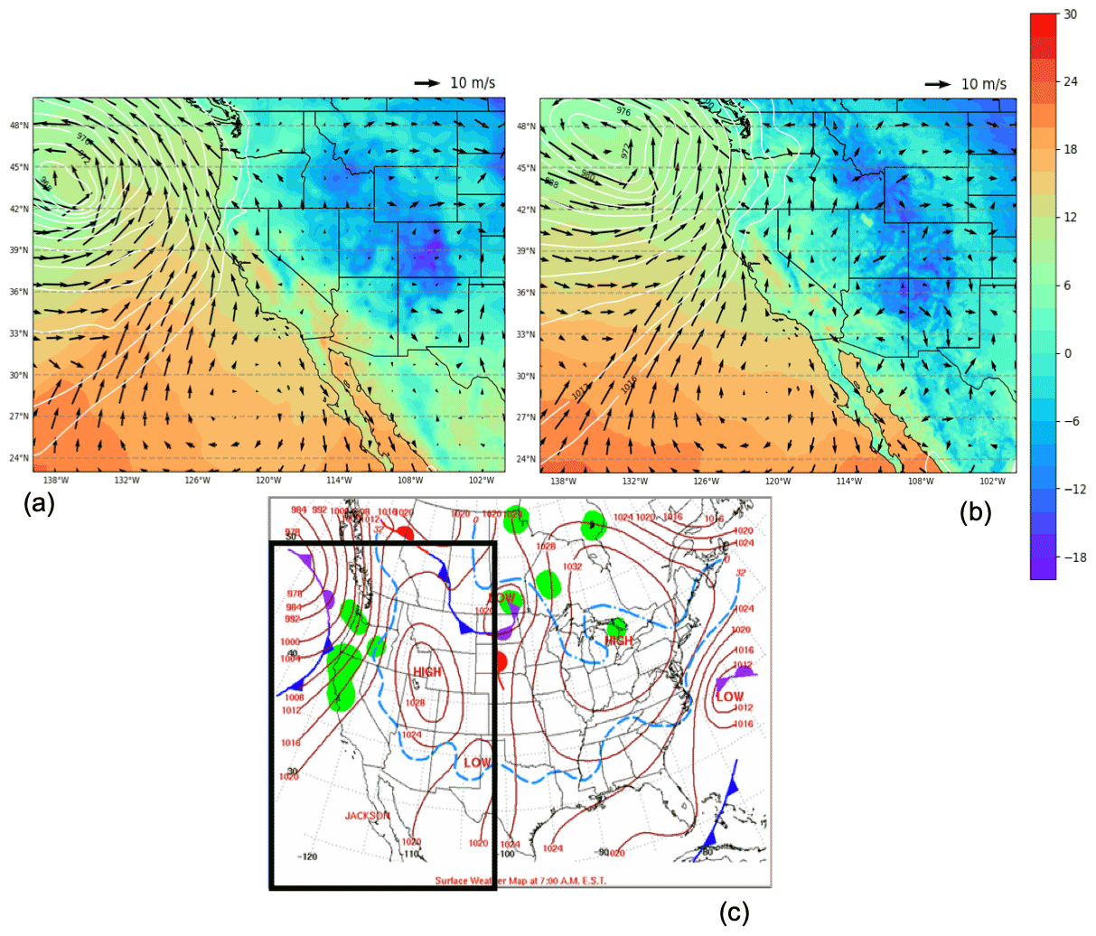
Figure 4(a, b) Mean sea level pressure (mslp, hPa, white contour lines), surface temperature (color shading, ∘C) and 100 m wind direction (black arrows, m s−1) at 07:00 UTC, 16 February 2004, of ERA5 reanalysis and RegCM 12 km, respectively. (c) NCEP-NOAA Surface Analysis of pressure and fronts. The black box in (c) bounds the area represented in (a) and (b).
The intermediate-resolution (12 km) domain (Fig. 3a) covers a wide area encompassing California and a large portion of the coastal Pacific Ocean, with 23 vertical levels and a parameterization for deep convection based on the Kain–Fritsch scheme (Kain, 2004). The ERA-Interim driven simulation is initialized at 00:00 UTC, 15 February 2004 (Table 2), and lasts until 00:00 UTC, 19 February 2004. This simulation is used as boundary conditions for a RegCM4-NH run over a smaller area centered over northern California (Fig. 3a) at 3 km horizontal resolution, with 41 vertical levels and boundary conditions updated every 6 h. In RegCM4-NH only the shallow convection code of the Tiedtke scheme (Tiedtke, 1996) is activated. Simulated precipitation is compared with the CHIRPS, CMORPH, TRMM, PRISM and NCEP/CPC observations (Table 3).
As shown in Fig. 4 the 16 February synoptic conditions for mean sea level pressure (mslp), surface temperature and wind direction of this case study are well reproduced by RegCM4 at 12 km (Fig. 4b) when compared to ERA5 reanalysis (Fig. 4a). The surface analysis of pressure and fronts derived from the operational weather maps prepared at the National Centers for Environmental Prediction, Hydrometeorological Prediction Center and National Weather Service (https://www.wpc.ncep.noaa.gov/dailywxmap/index_20040216.html, last access: 15 December 2021) is also reported in Fig. 4c.
The available observed precipitation datasets show similar patterns for the total accumulated precipitation (Fig. 5); in particular CHIRPS (Fig. 5a), PRISM (Fig. 5d) and NCEP (Fig. 5e) exhibit similar spatial details and magnitudes of extremes. CHIRPS shows a maximum around 42∘ N which is not found in the other datasets. CMORPH (Fig. 5b) and TRMM (Fig. 5c) show lower precipitation maxima and lesser spatial details due to their lower resolution, indicating that the performance of satellite-based products may be insufficient as a stand-alone product to validate the model for this case.
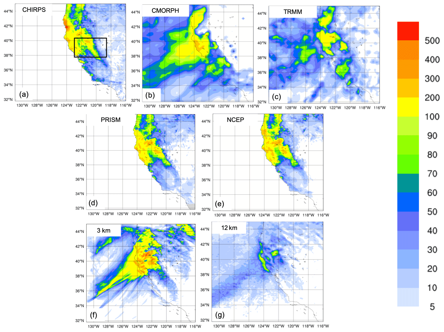
Figure 5Total accumulated precipitation (mm) during the California case: CHIRPS (a), CMORPH (b), TRMM (c) observations, PRISM (d), NCEP Reanalysis (e), and convection-permitting simulation with RegCM4-NH at 3 km (f) and RegCM4 at 12 km (g). The black box denotes the area where the spatial average of 6-hourly accumulated precipitation is calculated for Fig. 6a.
The largest observed maxima are placed on the terrain peaks, with extreme rainfall greater than 250 mm in 60 h over the coastal mountains and between 100–175 mm elsewhere (Fig. 5). The black box in Fig. 5a shows the area of the Russian River watershed where the largest rainfall rates were detected (269 and 124 mm in 60 h accumulated rainfall between 00:00 UTC, 16 February, and 12:00 UTC, 18 February 2004, respectively) (Ralph et al., 2006).
The convection-permitting simulation captures the basic features of the observed precipitation, both in terms of spatial distribution (Fig. 5f) and of temporal evolution of rainfall (Fig. 6a). However, it shows higher precipitation rates than observed over the sea and over the mountain chains, with lower intensities than observed in the southeast part of the mountain chain (Fig. 5). The 12 km simulation instead severely underestimates the magnitude of the event (Fig. 5g).
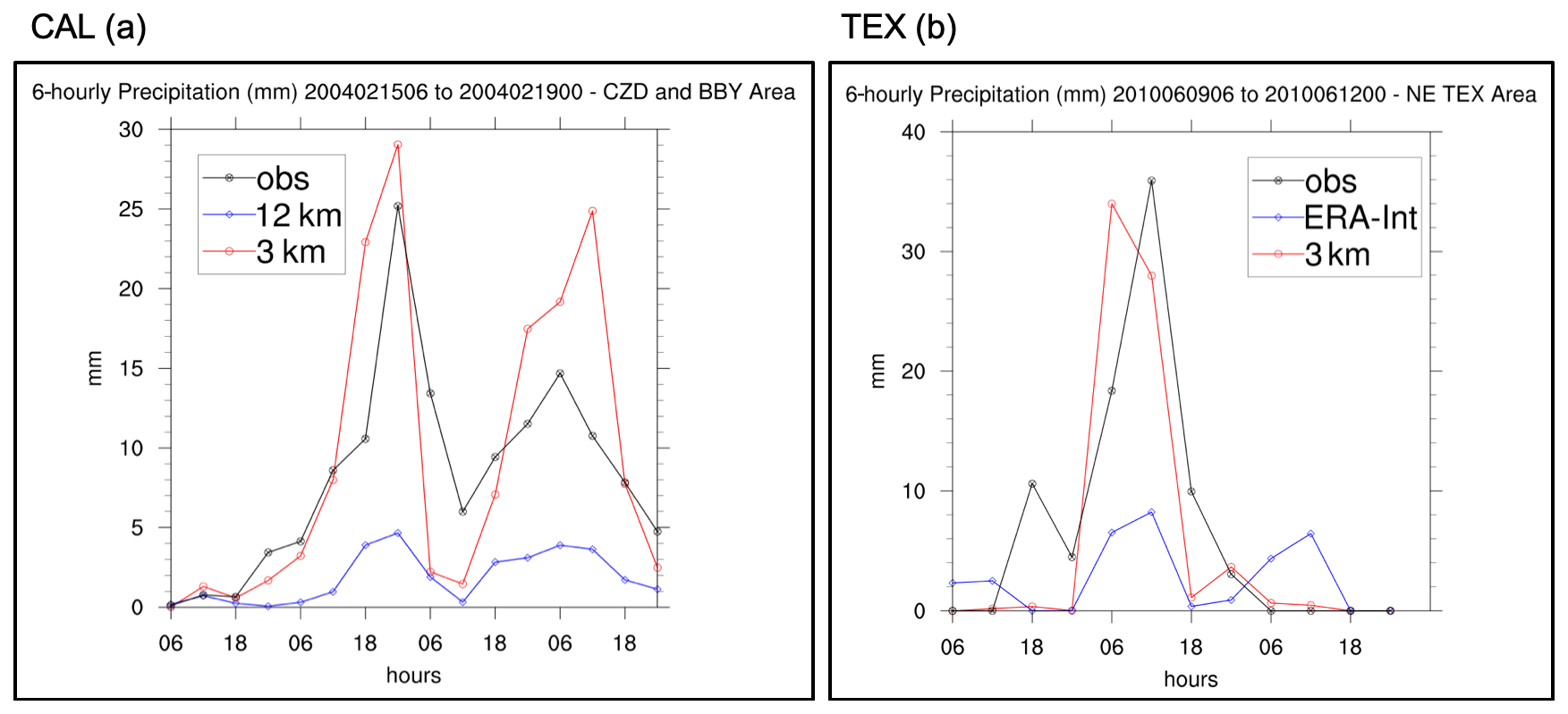
Figure 6Time series of the 6-hourly accumulated precipitation (in mm on the y axis) during the CAL event (a) and during the TEX event (b). The blue lines show RegCM4 12 km and ERA interim 6-hourly accumulated precipitation averaged over the areas indicated by the black squares in Figs. 5 and 7, while the red line shows the 6-hourly accumulated precipitation simulated by RegCM4-NH. The observations are shown with a black line.
Figure 6a shows the 6-hourly accumulated precipitation averaged over the black box in Fig. 5a. The 3 and 12 km simulations capture the onset of the event, but the peak intensity is strongly underestimated by the 12 km run, while it is well simulated by the 3 km run, although the secondary maximum is overestimated. These results demonstrate that only the high-resolution convection-permitting model is able to captures this extreme event and that parameterized convection has severe limits in this regard (Done et al., 2004; Lean et al., 2008; Weisman et al., 2008; Weusthoff et al., 2010; Schwartz, 2014; Clark et al., 2016).
Case 2, hereafter referred to as TEX (Table 2), is a convective precipitation episode exhibiting characteristics of the “Maya Express” flood events, linking tropical moisture plumes from the Caribbean and the Gulf of Mexico to midlatitude flooding over the central United States (Higgins et al., 2011). During the TEX event, an upper-level cutoff low over northeastern Texas, embedded within a synoptic-scale ridge, moved slowly northeastward. Strong low-level flow and moisture transport from the western Gulf of Mexico progressed northward across eastern Texas. The event was characterized by low-level moisture convergence, weak upper-level flow, weak vertical wind shear and relatively cold air (center of cutoff low), which favored the slow-moving convective storms and nearly stationary thunderstorm outflow boundaries. The main flooding event in eastern Texas occurred on 10 June 2010, with a daily maximum rainfall of 216.4 mm for the region in the black box of Fig. 7a (Higgins et al., 2011).

Figure 7Total accumulated precipitation (mm) during the Texas case: CHIRPS (a), CMORPH (b), TRMM (c), PRISM (d), NCEP Reanalysis (e), and convection-permitting simulation with RegCM4-NH at 3 km grid spacing (f) and ERA-Interim (g). The black box (a) shows the area where the spatial average of 6-hourly accumulated precipitation was calculated for Fig. 6b.
As for the California case, the observed precipitation datasets show coherent patterns for the total accumulated precipitation (Fig. 7), with the highest values related to the mesoscale convective system in eastern Texas (∼ 200 mm), and another smaller area of high precipitation more to the north, approximately over Oklahoma. PRISM (Fig. 7d) and NCEP (Fig. 7e) capture similar spatial details and magnitudes of extremes, and CHIRPS (Fig. 7a) has lower precipitation extremes in the north compared to the other datasets, while CMORPH (Fig. 7b) and TRMM (Fig. 7c) show the lowest precipitation extremes and reduced spatial details as already noted for the California case.
Figure 7f and g present precipitation as produced by the RegCM4-NH and the ERA-Interim reanalysis (driving data), respectively. ERA-Interim reproduces some of the observed features of precipitation but with a substantial underestimation over the areas of maximum precipitation because of its coarse resolution. By comparison, the RegCM4-NH simulation (Fig. 7f) shows an improvement in both pattern and intensity of precipitation and is substantially closer to observations over eastern Texas. However, the precipitation area is slightly overestimated and the model is not capable of reproducing the small region of maximum precipitation in the north.
The time series of precipitation over eastern Texas from 9–12 June 2010 for observations (black line), ERA-Interim (blue line) and RegCM4-NH (red line) are reported in Fig. 6b. Precipitation increases over this region from 00:00 UTC until it reaches the observed maximum at 12:00 UTC on 10 June (∼ 35 mm), gradually decreasing afterwards until 06:00 UTC on 11 June. The RegCM4-NH simulation shows a more realistic temporal evolution than the ERA-Interim, which exhibits an overall underestimation of precipitation. The non-hydrostatic model produces precipitation values closer to the observations; however, the simulated maximum is reached 6 h earlier than observed.
Case 3 focuses on Lake Victoria (LKV), with the purpose of testing RegCM4-NH on a complex and challenging region in terms of convective rainfall. It is estimated that each year 3000–5000 fishers perish on the lake due to nightly storms (IFRC, 2014). In the Lake Victoria basin, the diurnal cycle of convection is strongly influenced by lake–land breezes driven by the thermal gradient between the lake surface and the surrounding land. As the land warms during the course of the day, a lake breeze is generated which flows from the relatively cooler water towards the warmer land surface. The circulation is effectively reversed at night, when the land surface becomes cooler than the lake surface, leading to convergence over the lake and associated thermal instability.
In the LKV region, prevailing winds are generally easterly most of the year with some variability due to the movement of the Inter-Tropical Convergence Zone (ITCZ). The local diurnal circulation created by the presence of the lake creates two diurnal rainfall maxima. During daylight hours, when the lake breeze begins to advance inland, convergence is maximized on the eastern coast of the lake as the lake breeze interacts with the prevailing easterlies. Studies have also noted the importance of downslope katabatic winds along the mountains to the east of the lake in facilitating convergence along the eastern coastal regions (Anyah et al., 2006). This creates a maximum in rainfall and convection on the eastern coast of LKV. Conversely, during nighttime hours, when the local lake circulation switches to flow from the land towards the lake, the prevailing easterlies create locally strong easterly flow across the lake and an associated maximum in convergence and rainfall on the western side of LKV.
The LKV simulation starts on 25 November 1999 and extends to the beginning of December 1999 (Table 2), covering a 5 d period which falls within the short rain season of East Africa. The choice of 1999, an El Niño–Southern Oscillation (ENSO)-neutral year, was made in order to focus the analysis on local effects, such as the diurnal convection cycle in response to the lake–land breeze, with no influence of anomalous large-scale conditions. A one-dimensional lake model (Hostetler et al., 1993; Bennington et al., 2014) interactively coupled to RegCM4-NH was utilized to calculate the lake surface temperature (LST), since lake–atmosphere coupling has been shown to be important for LKV (Sun et al., 2015; Song et al., 2004). This coupled lake model has already been used for other lakes, including Lake Malawi in southern Africa (Diallo et al., 2018). As with the other experiments, the boundary conditions are provided by a corresponding 12 km RegCM4 simulation employing the convection scheme of Tiedtke (1996).
At the beginning of the simulation, the LST over the lake is uniformly set to 26 ∘C and is then allowed to evolve according to the lake–atmosphere coupling. This initial LST value is based on previous studies. For example, Talling (1969) finds Lake Victoria surface temperatures ranging from 24.5–26 ∘C during the course of the year. Several studies have used RCMs to investigate the Lake Victoria climate (Anyah et al., 2006; Anyah and Semazzi, 2009; Sun et al., 2015) and found a significant relationship between lake temperature and rainfall depending on season. The value of 26 ∘C is typical of the winter season and was chosen based on preliminary sensitivity tests using different values of initial temperature ranging from 24 to 26 ∘C.
The synoptic feature favorable for the production of precipitation over the LKV in this period corresponds to a large area of southeasterly flow from the Indian Ocean (Fig. 8a), which brings low-level warm moist air into the LKV region facilitating the production of convective instability and precipitation. This synoptic situation, with a low-level southeasterly jet off the Indian Ocean, is a common feature associated with high precipitation in the area (Anyah et al., 2006) and can be seen in ERA5 data (Fig. 8a). Although there is some bias in terms of magnitude, this is reasonably well reproduced by the 12 km simulation (Fig. 8b).
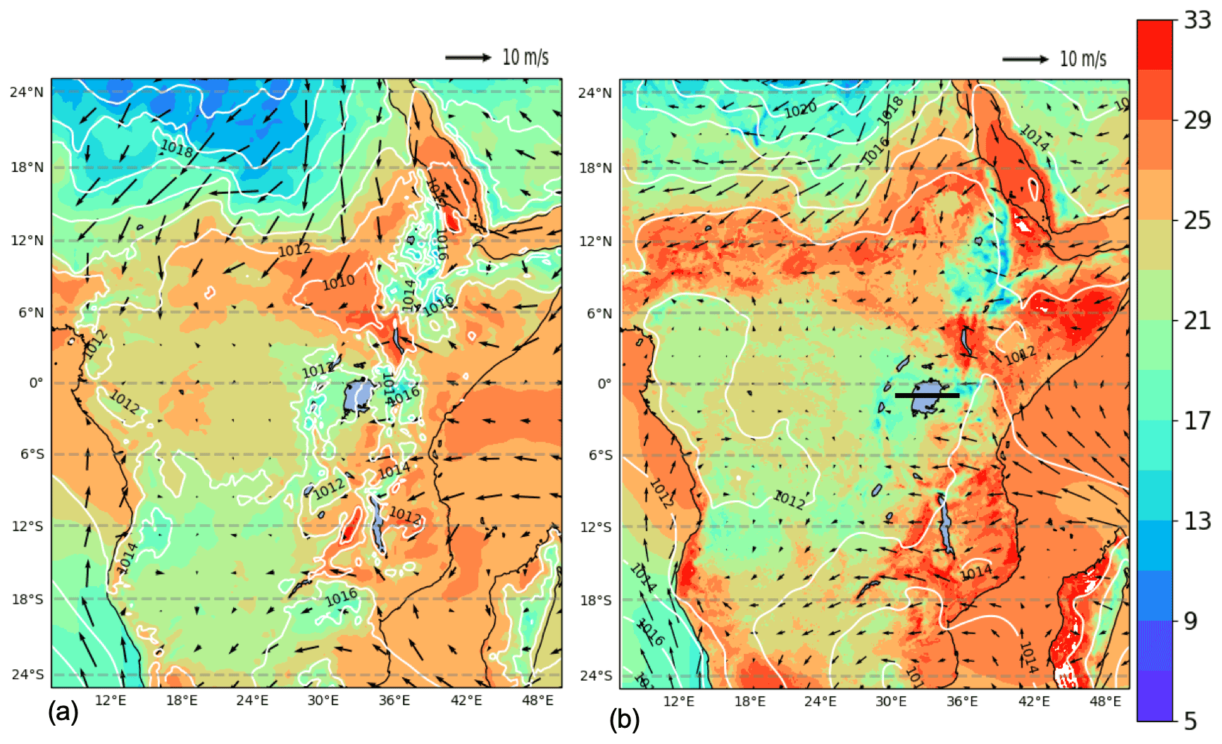
Figure 8Mean sea level pressure (mslp) (hPa) (white contour lines), surface temperature (color shading) (∘C) and 100 m wind (black arrows) averaged over the period 25 November, 00:00 UTC–1 December, 00:00 UTC, by ERA5 reanalysis (a) and RegCM 12 km (b). The black line (b) shows the cross-section position represented in Fig. 9.
The LKV region dynamics are quite distinct between nighttime and daytime and the rainfall in and around the lake has a pronounced diurnal cycle. To understand this strong diurnal cycle, Fig. 9 shows a cross section through the lake (32 to 34∘ E, black line in Fig. 8b) along 1∘ S latitude at a period during strong nighttime (Fig. 9b, d; 06:00 Z, 30 November) and daytime convection (Fig. 9a, c; 12:00 Z, 29 November). Wind vectors in Fig. 9 show the zonal-wind anomaly across 0–2∘ S to highlight the circulations associated with LKV. During the day, surface heating around the lake leads to a temperature difference between the land and lake sufficient to generate a lake breeze, which causes divergence over the lake, while over the highlands to the east the environment is more conducive to convection where convergence is focused (Fig. 9a, c). Conversely, during the night, a land breeze circulation is generated, which induces convergence and convection over the lake (Fig. 9b, d). In Fig. 10, the evolution of the nighttime land breeze is illustrated with cooler temperature anomalies propagating westward onto the lake during the night.
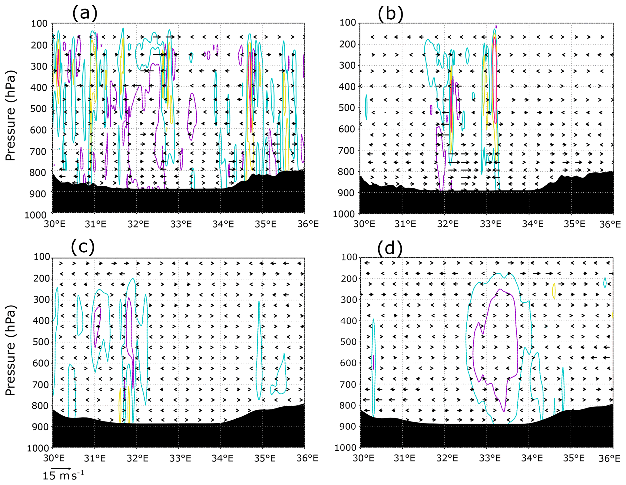
Figure 9Cross section through 1∘ S (black line in Fig. 8b) of the zonal-wind anomaly (0–2∘ S) vectors and the mean contoured vertical velocity (m s−1) over 0–2∘ S at (a) 12:00 Z, 29 November, and (b) 06:00 Z, 30 November, from the 3 km simulation. Purple dashed contours indicate −0.1 m s−1, light blue contours indicate 0.1 m s−1, yellow contours indicate 0.3 m s−1, and red contours indicate 0.5 m s−1. Lake Victoria extends from about 32 to 34∘ E. The bottom two panels show the same as in (a) and (b) but from the 12 km simulation at (c) 12:00 Z, 29 November, and (d) 06:00 Z, 30 November. Purple dashed contours indicate −0.01 hPa s−1, light blue dashed contours indicate −0.005 hPa s−1, and yellow dashed contours indicate 0.005 hPa s−1.
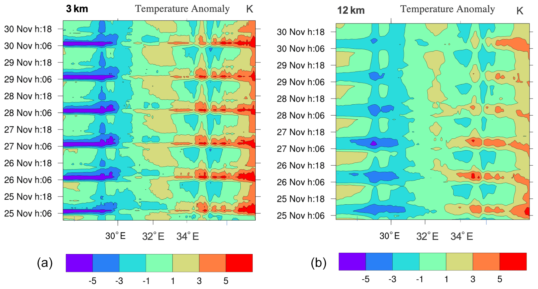
Figure 10Longitude–time (hourly) Hovmöller diagram of LKV domain surface temperature anomaly (shading, in K). Panels correspond to the 3 km simulation (a) and 12 km simulation (b). Lake Victoria is situated between 32 and 34∘ E longitude.
Comparing the 3 km simulation to the 12 km forcing run, we find that the localized circulations created by local forcings (i.e., convection) are much stronger in the convection-permitting resolution experiment. We also find stronger and more localized areas of convective updrafts compared to the 12 km simulation (Fig. 9c, d; ω is shown instead of vertical velocity here because of the difference in dynamical core). As an example during the nighttime event (Fig. 9b, d) there is a broad area of upward motion over the lake and the associated broad convergence in the 12 km simulation, while in the convection-permitting 3 km simulation, convection is much more local and concentrated over the western part of the lake. Indeed, nighttime rainfall tends to be concentrated over the western part of the lake (Sun et al., 2015; Fig. 11a–d). Stronger convection simulated in the 3 km experiment could also be tied to stronger temperature anomalies shown over the lake and land and between day and night relative to the 12 km simulation (Fig. 10). The 3 km simulation also shows a more pronounced land breeze propagation at night compared to the 12 km simulation.

Figure 11Total event accumulated precipitation (mm) during the LKV case (25 November 1999–1 December 1999) measured by CHIRPS (a), CMORPH (b), CPC (d) and TRMM (e) and calculated by RegCM4 at 3 km (e) and 12 km (f).
This demonstrates that the 3 km simulation is better equipped to simulate the localized circulations associated with this complex land–lake system.
Figure 11 reports the total accumulated precipitation observed and simulated for the LKV case. TRMM (Fig. 11d) and CPC (Fig. 11c) show a similar pattern, with two rainfall maxima of different intensities over the southeastern and northwestern lake areas. CMORPH (Fig. 11b) shows a western rainfall maximum similar to TRMM and one large rainfall area almost entirely centered over the highlands to the west of the lake. Conversely in CHIRPS (Fig. 11a) a maximum is found to the east of the lake, while several localized maxima occur over the lake. The differences among the observed datasets highlight the issue of observational uncertainty and the need to take into consideration shortcomings associated with the types of observational datasets considered. Different datasets can have significantly different climatologies, especially in areas of low data availability. For example, Prein and Gobiet (2017) analyzed two gauge-based European-wide datasets and seven global low-resolution datasets and found large differences across the observation products, often of similar magnitude as the difference among model simulations. In this case and for this area the observation uncertainty plays a big role especially at high resolution and highlights the need for an adequate observational network for model validation. However, despite the large uncertainty among the different observed datasets (Fig. 11a–d), we find a significant underestimation of the precipitation by the 12 km run over the lake independently of the dataset used as a reference (Fig. 11f). In contrast, the 3 km simulation (Fig. 11e) shows substantially greater detail, with rainfall patterns more in agreement with the CMORPH data. In particular, the 3 km simulation reproduces the local rainfall maxima well on the western side of the lake, although these appear more localized and with a multi-cell structure compared to CMORPH and TRMM. Additionally, the 12 km simulation underestimates the observed heavy rainfall totals in the highlands to the west of the lake region especially when compared to CMORPH, which are instead reproduced by the 3 km simulation.
This last test case demonstrates the ability of RegCM4-NH in simulating realistic convective activity over such a morphologically complex region, which is a significant improvement compared to the hydrostatic coarse-resolution model configuration.
In this paper we have described the development of RegCM4-NH, a non hydrostatic version of the regional model system RegCM4, which was completed in response to the need of moving to simulations at convection-permitting resolutions of a few kilometers. The non-hydrostatic dynamical core of MM5 has been incorporated into the RegCM4 system previously based on the MM5 hydrostatic core. Some modifications to the MM5 dynamical core were also implemented to increase the model stability for long-term runs. RegCM4-NH also includes two explicit cloud microphysics schemes needed to explicitly describe convection and cloud processes in the absence of the use of cumulus convection schemes. Finally, we presented a few case studies of explosive convection to illustrate how the model provides realistic results in different settings and general improvements compared to the coarser-resolution hydrostatic version of RegCM4 for such types of events.
As already mentioned, RegCM4-NH is currently being used for different projects and within these contests, is being run at grid spacings of a few kilometers for continuous decadal simulations, driven by reanalyses of observations or GCM boundary conditions (with the use of an intermediate-resolution domains) over different regions, such as the Alps, the Eastern Mediterranean, central eastern Europe and the Caribbean. These projects, involving multi-model inter-comparisons, indicate that the performance of RegCM4-NH is generally in line with that of other convection-permitting models and exhibits similar improvements compared to coarser-resolution models, such as a better simulation of the precipitation diurnal cycle and of extremes at hourly to daily timescales. The results obtained within the multi-model context confirm previous results from single-model studies (Kendon et al., 2012, 2017; Ban et al., 2014, 2015; Prein et al., 2015, 2017) but also strengthen the robustness of the findings through reduced uncertainty compared to coarse-resolution counterparts (Ban et al., 2021; Pichelli et al., 2021). The convection-permitting scale can thus open the perspective of more robust projections of future changes in precipitation, especially over sub-daily timescales.
One of the problems of the RegCM4-NH dynamical core is that, especially for long runs with varied meteorological conditions, a relatively short time step is needed for stability reasons. This makes the model rather computationally demanding, although not more than other convection-permitting modeling systems such as the Weather Research and Forecast model (WRF, Skamarock et al., 2008). For this reason, we are currently incorporating within the RegCM system a very different and more computationally efficient non-hydrostatic dynamical core, which will provide the basis for the next version of the model, RegCM5, to be released in the future.
Following the philosophy of the RegCM modeling system, RegCM4-NH is intended to be a public, free, open-source community resource for external model users. The non-hydrostatic dynamical core has been implemented in such a way that it can be activated in place of the hydrostatic dynamics through a user-set switch, which makes the use of RegCM4-NH particularly simple and flexible. We therefore envision that the model will be increasingly used by a broad community so that a better understanding can be achieved of its behavior, advantages and limitations.
Code is available at https://doi.org/10.5281/zenodo.4603556 (Giorgi et al. 2021). Case study configuration files are found at https://doi.org/10.5281/zenodo.5106399 (Coppola et al. 2021).
EC prepared the paper with contributions from all co-authors, and EC also coordinated the research, PS, JATA and RG carried out and analyzed the simulations. EP investigated solutions to stabilize/adapt the model at the kilometer scale and performed preliminary validation tests. GG developed/adapted the model code. FDS contributed to developing the coupled version of the model. RN developed one of the microphysics schemes. FG supervised and coordinated all activities.
The contact author has declared that neither they nor their co-authors have any competing interests.
Publisher's note: Copernicus Publications remains neutral with regard to jurisdictional claims in published maps and institutional affiliations.
This paper was edited by Astrid Kerkweg and reviewed by two anonymous referees.
Anthes, R. A., Hsie, E.-Y., and Kuo, Y. -H.: Description of the Penn State/NCAR Mesoscale Model: Version 4 (MM4), National Center for Atmospheric Research, Boulder, CO, USA, NCAR Techn. Note, 4, 79 pp., NCAR/TN-282+STR, https://doi.org/10.5065/D64B2Z90, 1987.
Anyah, R., Semazzi, F. H. M., and Xie, L.: Simulated Physical Mechanisms Associated with Climate Variability over Lake Victoria Basin in East Africa, Mon. Weather Rev., 134, 3588–3609, 2006.
Anyah, R. O. and Semazzi, F.: Idealized simulation of hydrodynamic characteristics of Lake Victoria that potentially modulate regional climate, Int. J. Climatol., 29, 971–981, https://doi.org/10.1002/joc.1795, 2009.
Ashouri, H., Hsu, K., Sorooshian, S., Braithwaite, D. K., Knapp, K. R., Cecil, L. D., Nelson, B. R., and Prat, O. P.: PERSIANN-CDR: Daily Precipitation Climate Data Record from Multisatellite Observations for Hydrological and Climate Studies, Bull. Am. Meteorol. Soc., 96, 69–83, https://doi.org/10.1175/BAMS-D-13-00068.1, 2015.
Ban, N., Schmidli, J., and Schär, C.: Evaluation of the convection-resolving regional climate modeling approach in decade-long simulations, J. Geophys. Res.-Atmos., 119, 7889–7907, https://doi.org/10.1002/2014JD021478, 2014.
Ban, N., Schmidli, J., and Schär ,C.: Heavy precipitation in a changing climate: does short-term summer precipitation increase faster?, Geophys. Res.-Lett., 42, 1165–1172, https://doi.org/10.1002/2014GL062588, 2015.
Ban, N., Caillaud, C., Coppola, E., Pichelli, E., Sobolowski, S., Adinolfi, M., Ahrens, B., Alias, A., Anders, I., Bastin, S., Belušić, D., Berthou, S., Brisson, E., Cardoso, R. M., Chan, S. C., Bøssing Christensen, O., Fernández, J., Fita, L., Frisius, T., Gašparac, G., Giorgi, F., Goergen, K., Haugen, J. E., Hodnebrog, Ø., Kartsios, S., Katragkou, E., Kendon, E. J., Keuler, K., Lavin-Gullon, A., Lenderink, G., Leutwyler, D., Lorenz, T., Maraun, D., Mercogliano, P., Milovac, J., Panitz, H.-J., Raffa, M., Reca Remedio, A., Schär, C., Soares, P. M. M., Srnec, L., Steensen, B. M., Stocchi, P., Tölle, M. H., Truhetz, H., Vergara-Temprado, J., de Vries, H., Warrach-Sagi, K., Wulfmeyer, V., and Zander, M. J.: The first multi-model ensemble of regional climate simulations at kilometer-scale resolution, part I: evaluation of precipitation, Clim. Dynam., 57, 275–302, https://doi.org/10.1007/s00382-021-05708-w, 2021.
Beheng, K.: A parameterization of warm cloud microphysical conversion processes, Atmos. Res., 33, 193–206, 1994.
Bennington, V., Notaro, M., and Holman, K. D.: Improving Climate Sensitivity of Deep Lakes within a Regional Climate Model and Its Impact on Simulated Climate, J. Climl., 27, 2886–2911, 2014.
Bretherton, C. S., McCaa, J. R., and Grenier, H.: A new parameterization for shallow cumulus convection and its application to marine subtropical cloud-topped boundary lay-ers. I. Description and 1D results, Mon. Weather Rev., 132, 864–882, 2004.
Chen, M., Shi, W., Xie, P., Silva, V. B. S., Kousky, V. E., Higgins, R. W., and Janowiak, J. E.: Assessing objective techniques for gauge-based analyses of global daily precipitation, J. Geophys. Res., 113, D04110, https://doi.org/10.1029/2007JD009132, 2008.
Clark, P., Roberts, N., Lean, H., Ballard, S. P., and Charlton-Perez, C.: Convection-permitting models: A step-change in rainfall forecasting, Meteor. Appl., 23, 165–181, https://doi.org/10.1002/met.1538, 2016.
Coppola, E., Giorgi, F., Mariotti, L., and Bi, X.: RegT-Band: a tropical band version of RegCM4, Clim. Res., 52, 115–133, 2012.
Coppola, E., Sobolowski, S., Pichelli, E., Pichelli, E., Raffaele, F., Ahrens, B., Anders, I., Ban, N., Bastin, S., Belda, M., Belusic, D., Caldas-Alvarez, A., Cardoso, R. M., Davolio, S., Dobler, A., Fernandez, J., Fita, L., Fumiere, Q., Giorgi, F., Goergen, K., Güttler, I., Halenka, T., Heinzeller, D., Hodnebrog, Ø., Jacob, D., Kartsios, S., Katragkou, E., Kendon, E, Khodayar, S., Kunstmann, H., Knist, S., Lavín-Gullón, A., Lind, P., Lorenz, T., Maraun, D., Marelle, L., van Meijgaard, E., Milovac, J., Myhre, G., Panitz, H.-J., Piazza, M., Raffa, M., Raub, T., Rockel, B., Schär, C., Sieck, K., Soares, P. M. M., Somot, S., Srnec, L., Stocchi, P., Tölle, M. H., Truhetz, H., Vautard, R., de Vries, H., and Warrach-Sagi, K.: A first-of-its-kind multi-model convection permitting ensemble for investigating convective phenomena over Europe and the Mediterranean, Clim. Dynam., 55, 3–34, https://doi.org/10.1007/s00382-018-4521-8, 2020.
Coppola, E., Stocchi, P., Pichelli, E., Torres, A., Glazer, R., Graziano, G., Di Sante, F., Nogherotto, R., and Giorgi, F.: RegCM-NH namelists for test cases presented in the paper “Non-Hydrostatic RegCM4 (RegCM4-NH): Model description and case studies over multiple domains”, Zenodo [code], https://doi.org/10.5281/zenodo.5106399, 2021.
Dacre, H. F., Clark, P. A., Martinez-Alvarado, O., Stringer, M. A., and Lavers, D. A.: How do atmospheric rivers form?, Bull. Amer. Meteorol. Soc., 96, 1243–1255, https://doi.org/10.1175/BAMS-D-14-00031.1, 2015.
Dee, D. P., Källén, E., Simmons, A. J., and Haimberger, L.: Comments on “Reanalyses suitable for characterizing long-term trends”, B. Am. Meteorol. Soc., 92, 65–70, https://doi.org/10.1175/2010BAMS3070.1, 2011.
Diallo, I., Giorgi, F., and Stordal, F.: Influence of Lake Malawi on regional climate from a double nested regional climate model experiment, Clim. Dynam., 50, 3397–3411, https://doi.org/10.1007/s00382-017-3811-x, 2018.
Dickinson, R. E., Errico, R. M., Giorgi, F., and Bates, G. T.: A regional climate model for the western United States, Climatic Change, 15, 383–422, https://doi.org/10.1007/BF00240465, 1989.
Dickinson, R. E., Henderson-Sellers, A., and Kennedy, P.: Biosphere–atmosphere transfer scheme (BATS) version 1e as coupled to the NCAR community climate model, TechRep, National Center for Atmospheric Research, Boulder, CO, USA, 80 pp., NCAR.TN-387+STR, 1993.
Done, J., Davis, C. A., and Weisman M. L.: The next generation of NWP: Explicit forecasts of convection using the Weather Research and Forecasting (WRF) model, Atmos. Sci. Lett., 5, 110–117, https://doi.org/10.1002/asl.72, 2004.
Dudhia, J.: Numerical study of convection observed during the winter monsoon experiment using a mesoscale two-dimensional model, J. Atmos. Sci., 46, 3077–3107, 1989.
Durran, D. R. and Klemp, J. B.: A compressible model for the simulation of moist mountain waves, Mon. Weather Rev., 111, 2341–2361, 1983.
Elguindi, N., Bi, X., Giorgi, F., Nagarajan, B., Pal, J., Solmon, F., Rauscher, S., Zakey, S., O'Brien, T., Nogherotto, R., and Giuliani, G.: Regional Climate Model, RegCM Reference Manual Version 4.7, 49 pp., https://zenodo.org/record/4603616, 2017.
Emanuel, K. A.: A scheme for representing cumulus convection in large-scale models, J. Atmos. Sci, 48, 2313–2335, 1991.
Fairall, C. W., Bradley, E. F., Godfrey, J. S., Wick, G. A., Edson, J. B., and Young, G. S.: The cool skin and the warm layer in bulk flux calculations, J. Geophys. Res., 101, 1295–1308, 1996a.
Fairall, C. W., Bradley, E. F., Rogers, D. P., Edson, J. B., and Young, G. S.: Bulk parameterization of air-sea fluxes for TOGA COARE, J. Geophys. Res., 101, 3747–3764, 1996b.
Funk, C., Peterson, P., Landsfeld, M., Pedreros, D., Verdin, J., Shukla, S., Husak, G., Rowland, J., Harrison, L., Hoell, A., and Michaelsen, J.: The climate hazards infrared precipitation with stations–a new environmental record for monitoring extremes, Sci. Data, 2, 150066, https://doi.org/10.1038/sdata.2015.66, 2015.
Gimeno, L., Nieto, R., Vaìsquez, M., and Lavers, D. A.: Atmospheric rivers: A mini-review, Front. Earth Sci., 2, 1–6, https://doi.org/10.3389/feart.2014.00002, 2014.
Giorgi, F.: Thirty years of regional climate modeling: where are we and where are we going next?, J. Geophys. Res.-Atmos., 124, 5696–5723, 2019.
Giorgi, F. and Bates, G. T.: The Climatological Skill of a Regional Model over Complex Terrain, Mon. Weather Rev., 117, 2325–2347, https://doi.org/10.1175/1520-0493(1989)117<2325:TCSOAR>2.0.CO;2, 1989.
Giorgi, F. and Mearns, L. O.: Introduction to special section: regional climate modeling revisited, J. Geophys. Res., 104, 6335–6352, 1999.
Giorgi, F., Marinucci, M. R., and Bates, G.: Development of a second generation regional climate model (RegCM2). I. Boundary layer and radiative transfer processes, Mon. Weather Rev., 121, 2794–2813, 1993a.
Giorgi, F., Marinucci, M. R., Bates, G., and De Canio, G.: Development of a second generation regional climate model (RegCM2), part II: convective processes and assimilation of lateral boundary conditions, Mon. Weather Rev., 121, 2814–2832, 1993b.
Giorgi, F., Francisco, R., and Pal, J. S.: Effects of a sub-gridscale topography and landuse scheme on surface climateand hydrology. I. Effects of temperature and water vapor disaggregation, J. Hydrometeorol., 4, 317–333, 2003.
Giorgi, F., Jones, C., and Asrar, G.: Addressing climate information needs at the regional level: the CORDEX framework, WMO Bull., 58, 175–183, 2009.
Giorgi, F., Coppola, E., Solmon, F., Mariotti, L., Sylla, M. B., Bi, X., Elguindi, N., Diro, G. T., Nair, V., Giuliani, G., Turuncoglu, U. U., Cozzini, S., Güttler, I., O'Brien, T. A., Tawfik, A. B., Shalaby, A., Zakey, A. S., Steiner, A. L., Stordal, F., Sloan, L. C., and Brankovic, C.: RegCM4: model description and preliminary tests over multiple CORDEX domains, Clim. Res., 52, 7–29, https://doi.org/10.3354/cr01018, 2012.
Giorgi, F., Solmon, F., Xunjang, B., Coppola, E., Giuliani, G., Turunçoğlu, U., Güttler, I., Mariotti, L., Nogherotto, R., O'Brien, T. A., Tawfik, A., Elguindi, N., Piani, S., Pal, J., Tefera Diro, G., and Shalaby, A.: ictp-esp/RegCM: Paper Release, Zenodo [code], https://doi.org/10.5281/zenodo.4603556, 2021.
Grell, G. A.: Prognostic evaluation of assumptions used by cumulus parameterizations, Mon. Weather Rev., 121, 764–787, 1993.
Grell, G. A., Dudhia J., and Stauffer, D. R.: A Description of the Fifth Generation Penn State/NCAR Mesoscale Model (MM5), National Center for Atmospheric Research, Boulder, CO, USA, NCAR Tech. Note, 122, NCAR/TN-398+STR 1994.
Gunn, K. L. S. and Marshall, J. S.: The distribution with size of aggregate snowflakes, J. Meteor., 15, 452–461, https://doi.org/10.1175/1520-0469(1958)015<0452:TDWSOA>2.0.CO;2, 1958.
Gutowski Jr., W. J., Giorgi, F., Timbal, B., Frigon, A., Jacob, D., Kang, H.-S., Raghavan, K., Lee, B., Lennard, C., Nikulin, G., O'Rourke, E., Rixen, M., Solman, S., Stephenson, T., and Tangang, F.: WCRP COordinated Regional Downscaling EXperiment (CORDEX): a diagnostic MIP for CMIP6, Geosci. Model Dev., 9, 4087–4095, https://doi.org/10.5194/gmd-9-4087-2016, 2016.
Hewitt, C. D. and Lowe, J. A.: Toward a European climate prediction system, Bull. Amer. Meteor. Soc., 99, 1997–2001, https://doi.org/10.1175/BAMS-D-18-0022.1, 2018.
Higgins, R. W., Kousky, V. E., and Xie, P.: Extreme Precipitation Events in the South-Central United States during May and June 2010: Historical Perspective, Role of ENSO, and Trends, J. Hydrometeorol., 12, 1056–1070, https://doi.org/10.1175/JHM-D-10-05039.1, 2011.
Holtslag, A., de Bruijn, E., and Pan, H. L.: A high resolution air mass transformation model for short-range weather fore-casting, Mon. Weather Rev., 118, 1561–1575, 1990.
Hong, S.-Y., Juang, H.-M. H., and Zhao, Q.: Implementation of prognostic cloud scheme for a regional spectral model, Mon. Weather Rev., 126, 2621–2639, 1998.
Hong, S.-Y. and Lim, J.-O. J.: The WRF Single-Moment 6-Class Microphysics Scheme (WSM6), J. Korean Meteor. Soc., 42, 129–151, 2006.
Hong, S.-Y., Dudhia, J., and Chen, S.-H.: A Revised Approach to Ice Microphysical Processes for the Bulk Parameterization of Clouds and Precipitation, Mon. Weather Rev., 132, 103–120, 2004.
Hostetler, S. W., Bates, G. T., and Giorgi, F.: Interactive nesting of a lake thermal model within a regional climate model for climate change studies, J. Geophys. Res., 98, 5045–5057, 1993.
Huffman, G. J., Bolvin, D. T., Nelkin, E. J., Wolff, D. B., Adler, R. F., Gu, G., Hong, Y., Bowman, K. P., and Stocker, E. F.: The TRMM Multisatellite Precipitation Analysis (TMPA): Quasi-Global, Multiyear, Combined-Sensor Precipitation Estimates at Fine Scales, J. Hydrometeor., 8, 38–55, https://doi.org/10.1175/JHM560.1, 2007.
International Federation of Red Cross and Red Crescent Societies (IFRC): World Disasters Report 2014: focus on culture and risk. Technical Report, International Federation of Red Cross and Red Crescent Societies, Geneva, Switzerland, 276 pp., 2014.
Joyce, R. J., Janowiak, J. E., Arkin, P. A., and Xie, P.: CMORPH: A Method that Produces Global Precipitation Estimates from Passive Microwave and Infrared Data at High Spatial and Temporal Resolution, J. Hydrometeor, 5, 487–503, 2004.
Kain, J. S.: The Kain–Fritsch convective parameterization: An update, J. Appl. Meteor., 43, 170–181, https://doi.org/10.1175/1520-0450(2004)043<0170:TKCPAU>2.0.CO;2, 2004.
Kain, J. S. and Fritsch, J. M.: A one-dimensional entraining/detraining plume model and its application in convective parameterization, J. Atmos. Sci., 47, 2784–2802, 1990.
Kendon, E. J., Roberts, N. M., Senior, C. A., and Roberts, M. J.: Realism of rainfall in a very high-resolution regional climate model, J. Climate, 25, 5791–5806, https://doi.org/10.1175/JCLI-D-11-00562.1, 2012.
Kendon, E. J., Ban, N., Roberts, N. M., Fowler, H. J., Roberts, M. J., Chan, S. C., Evans, J. P., Fosser, G., and Wilkinson, J. M.: Do convection-permitting regional climate models improve projections of future precipitation change?, Bull. Amer. Meteor. Soc., 98, 79–93, https://doi.org/10.1175/BAMS-D-15-0004.1, 2017.
Kessler, E.: On the Distribution and Continuity of Water Substance in Atmospheric Circulations, in: Meteorological Monographs, Amer. Meteor. Soc., Boston, MA, 10, 84 pp., https://doi.org/10.1007/978-1-935704-36-2_1, 1969.
Khairoutdinov, M. and Kogan, Y.: A new cloud physics parameterization in a large-eddy simulation model of marine stratocumulus, Bull. Amer. Meteorol. Soc., 128, 229–243, 2000.
Kiehl, J., Hack, J., Bonan, G., Boville, B., Breigleb, B., Williamson, D., and Rasch, P.: Description of the NCAR Community Climate Model (CCM3), National Center for Atmospheric Research, Boulder, CO, USA, NCAR Tech. Note, NCAR, 159 pp., NCAR/TN-420+STR, 1996.
Klemp, J. B. and Lilly, D. K.: Numerical simulation of hydrostatic mountain waves, J. Atmos. Sci., 35, 78–107, 1978.
Klemp, J. B. and Dudhia, J.: An Upper Gravity-Wave Absorbing Layer for NWP Applications, Mon. Weather Rev., 176, 3987–4004, 2008.
Lean, H. W., Clark, P. A., Dixon, M., Roberts, N. M., Fitch, A., Forbes, R., and Halliwell, C.: Characteristics of high-resolution versions of the Met Office Unified Model for forecasting convection over the United Kingdom, Mon. Weather Rev., 136, 3408–3424, https://doi.org/10.1175/2008MWR2332.1, 2008.
LeVeque, R. J.: Finite Difference Methods for Ordinary and Partial Differential Equations, SIAM, Philadelphia, USA, https://doi.org/10.1137/1.9780898717839, 2007.
Lin, Y., Farley, R., and Orville, H.: Bulk parameterization of the snow field in a cloud model, J. Appl. Meteor. Clim., 22, 1065–1092, 1983.
Marshall, J. S. and Palmer, W. M. K.: The distribution of raindrops with size, J. Meteor., 5, 165–166, 1948.
Matte, D., Laprise, R., Thériault, J. M., and Lucas-Picher, P.: Spatial spin-up of fine scales in a regional climate model simulation driven by low-resolution boundary conditions, Clim. Dynam., 49, 563–574, https://doi.org/10.1007/s00382-016-3358-2, 2017.
Mlawer, E. J., Taubman, S. J., Brown, P. D., Iacono, M. J., and Clough, S. A.: Radiative transfer for inhomogeneous atmospheres: RRTM, a validated correlated-k model for the longwave, J. Geophys. Res., 102, 16663–16682, 1997.
Nogherotto, R., Tompkins, A. M., Giuliani, G., Coppola, E., and Giorgi, F.: Numerical framework and performance of the new multiple-phase cloud microphysics scheme in RegCM4.5: precipitation, cloud microphysics, and cloud radiative effects, Geosci. Model Dev., 9, 2533–2547, https://doi.org/10.5194/gmd-9-2533-2016, 2016.
Oleson, K. W., Lawrence, D. M., Bonan, G. B., Drewniak, B., Huang, M., Koven, C. D., Levis, S., Li, F., Riley, W. J., Subin, Z. M., Swenson, S. C., Thornton, P. E., Bozbiyik, A., Fisher, R., Kluzek, E., Lamarque, J.-F., Lawrence, P. J., Leung, L. R., Lipscomb, W., Muszala, S., Ricciuto, D. M., Sacks, W., Sun, Y., Tang, J., and Yang, Z.-L: Technical Description of version 4.5 of the Community Land Model (CLM), National Center for Atmospheric Research, Boulder, CO, USA, NCAR Techn. Note, 422 pp., NCAR/TN-503+STR, https://doi.org/10.5065/D6RR1W7M, 2013.
Pal, J. S., Small, E., and Eltahir, E.: Simulation of regional-scale water and energy budgets: representation of subgrid cloud and precipitation processes within RegCM, J. Geophys. Res., 105, 29579–29594, 2000.
Pal, J. S., Giorgi, F., Bi, X., Elguindi, N., Solmon, F., Gao, X., Rauscher, S. A., Francisco, R., Zakey, A., Winter, J., Ashfaq, M., Syed, F. S., Bell, J. L., Diffenbaugh, N. S., Karmacharya, J., Konaré, A., Martinez, D., da Rocha, R. P., Sloan, L. C., and Steiner, A. L.: The ICTP RegCM3 and RegCNET: regional climate modeling for the developing world., Bull. Amer. Meteorol. Soc., 88, 1395–1409, 2007.
Pichelli, E., Coppola, E., Sobolowski, S., Ban, N., Giorgi, F., Stocchi, P., Alias, A., Belušić, D., Berthou, S., Caillaud, C., Cardoso, R. M., Chan, S., Christensen, O. B., Dobler, A., de Vries, H., Goergen, K., Kendon, E. J., Keuler, K., Lenderink, G., Lorenz, T., Mishra, A. N., Panitz, H.-J., Schär, C, Soares, P. M. M., Truhetz, H., and Vergara-Temprado, J.: The first multi-model ensemble of regional climate simulations at kilometer-scale resolution part 2: historical and future simulations of precipitation, Clim. Dynam., 56, 3581–3602, https://doi.org/10.1007/s00382-021-05657-4, 2021.
Prein, A. F. and Gobiet, A.: Impacts of uncertainties in European gridded precipitation observations on regional climate analysis, Int. J. Climatol., 37, 305–327, https://doi.org/10.1002/joc.4706, 2017.
Prein, A. F., Langhans, W., Fosser, G., Ferrone, A., Ban, N., Goergen, K., Keller, M., Tölle, M., Gutjahr, O., Feser, F., Brisson, E., Kollet, S., Schmidli, J., van Lipzig, N. P. M., and Leung, R.: A review on regional convection-permitting climate modeling: demonstrations, prospects, and challenges, Rev. Geophys., 53, 323–361, 2015.
Ralph, F. M., Neiman, P. J., Wick, G. A., Gutman, S. I., Dettinger, M. D., Cayan, D. R., and White, A. B.: Flooding on California's Russian River: Role of atmospheric rivers, Geophys. Res. Lett., 33, L13801, https://doi.org/10.1029/2006GL026689, 2006.
Ralph, F. M., Dettinger, M. D., Cairns, M. M., Galarneau, T. J., and Eylander, J.: Defining “atmospheric river”: How the Glossary of Meteorology helped resolve a debate, Bull. Amer. Meteor. Soc., 99, 837–839, https://doi.org/10.1175/BAMS-D-17-0157.1, 2018.
Rutledge, S. A. and Hobbs, P. V.: The mesoscale and microscale structure and organization of clouds and precipitation in midlatitude cyclones. Part VIII: A model for the “seeder-feeder” process in warm-frontal rainbands, J. Atmos. Sci., 40, 1185–1206, 1983.
Schwartz, C. S.: Reproducing the September 2013 record-breaking rainfall over the Colorado Front Range with high-resolution WRF forecasts, Weather Forecast., 29, 393–402, https://doi.org/10.1175/WAF-D-13-00136.1, 2014.
Sitz, L. E., Sante, F., Farneti, R., Fuentes-Franco, R., Coppola, E., Mariotti, L., Reale, M., Sannino, G., Barreiro, M., Nogherotto, R., Giuliani, G., Graffino, G., Solidoro, C., Cossarini, G., and Giorgi, F.: Description and Evaluation of the Earth System Regional Climate Model (RegCM–ES), J. Adv. Model. Earth Sy., 9, 1863–1886, https://doi.org/10.1002/2017MS000933, 2017.
Skamarock, W. C., Klemp, J. B., Dudhia, J., Gill, D. O., Barker, D. M., Duda, M. G., Huang, X. Y., Wang, W., and Powers, J. G.: A description of the advanced research WRF version 3, National Center for Atmospheric Research, NCAR, Boulder, CO, USA, NCAR Techn. Note, 125 pp., NCAR/TN-475+STR, 2008.
Song, Y., Semazzi, H. M. F., Xie, L., and Ogallo, L. J.: A coupled regional climate model for the Lake Victoria Basin of East Africa, Int. J. Climatol., 24, 57–75, 2004.
Sun, X., Xie, L., Semazzi, F., and Liu, B.: Effect of Lake Surface Temperature on the Spatial Distribution and Intensity of the Precipitation over the Lake Victoria Basin, Mon. Weather Rev. 143, 1179–1192, 2015.
Sundqvist, H., Berge, E., and Kristjansson, J.: Condensation and cloud parameterization studies with a mesoscale numerical weather prediction model, Mon. Weather Rev., 117, 1641–1657, 1989.
Talling, J. F.: The incidence of vertical mixing, and some biological and chemical consequences, in: Tropical African lakes, Verh. Int. Ver. Limnol., 17, 998–1012, https://doi.org/10.1080/03680770.1968.11895946, 1969.
Tiedtke, M.: A comprehensive mass flux scheme for cumulus parametrization in large-scale models, Mon. Weather Rev., 117, 1779–1800, 1989.
Tiedtke, M.: Representation of Clouds in Large-Scale Models, Mon. Weather Rev., 121, 3040–3061, https://doi.org/10.1175/1520-0493(1993)121<3040:ROCILS>2.0.CO;2, 1993.
Tiedtke, M.: An extension of cloud-radiation parameterization in the ECMWF model: The representation of subgrid-scale variations of optical depth, Mon. Weather Rev., 124, 745–750, 1996.
Tompkins, A.: Ice supersaturation in the ECMWF integrated forecast system, Q. J. Roy. Meteor. Soc., 133, 53–63, 2007.
Tripoli, G. J. and Cotton, W. R.: A numerical investigation of several factors contributing to the observed variable intensity of deep convection over south Florida, J. Appl. Meteor., 19, 1037–1063, 1980.
Weisman, M. L., Davis, C., Wang, W., Manning, K. W., and Klemp, J. B.: Experiences with 0–36-h explicit convective forecasts with the WRF-ARW model, Weather Forecast., 23, 407–437, https://doi.org/10.1175/2007WAF2007005.1, 2008.
Weusthoff, T., Ament, F., Arpagaus, M., and Rotach, M. W.: Assessing the benefits of convection-permitting models by neighborhood verification: Examples from MAP D-PHASE, Mon. Weather Rev., 138, 3418–3433, https://doi.org/10.1175/2010MWR3380.1, 2010.
Williams, P. D.: A proposed modification to the Robert–Asselin time filter, Mon. Weather Rev., 137, 2538–2546, 2009.
Zeng, X., Zhao, M., and Dickinson, R. E.: Intercomparison of bulk aerodynamic algorithms for the computation of sea surface fluxes using TOGA COARE and TAO data, J. Clim., 11, 2628–2644, 1998.
Zhu, Y. and Newell, R. E.: A proposed algorithm for moisture fluxes from atmospheric rivers, Mon. Weather Rev., 126, 725–735, https://doi.org/10.1175/1520-0493(1998)126<0725:APAFMF>2.0.CO;2, 1998.