Bulk hydrometeor optical properties for microwave and sub-millimetre radiative transfer in RTTOV-SCATT v13.0

Satellite observations of radiation in the microwave and sub-millimetre spectral regions (broadly from 1 to 1000 GHz) can have strong sensitivity to cloud and precipitation particles in the atmosphere. These particles (known as hydrometeors) scatter, absorb, and emit radiation according to their mass, composition, shape, internal structure, and orientation. Hence, microwave and sub-millimetre observations have applications including weather forecasting, geophysical retrievals and model validation. To simulate these observations requires a scattering-capable radiative transfer model and an estimate of the bulk optical properties of the hydrometeors. This article describes the module used to integrate single-particle optical properties over a particle size distribution (PSD) to provide bulk optical properties for the Radiative Transfer for TOVS microwave and sub-millimetre scattering code, RTTOV-SCATT, a widely used fast model. Bulk optical properties can be derived from a range of particle models including Mie spheres (liquid and frozen) and non-spherical ice habits from the Liu and Atmospheric Radiative Transfer Simulator (ARTS) databases, which include pristine crystals, aggregates, and hail. The effects of different PSD and particle options on simulated brightness temperatures are explored, based on an analytical two-stream solution for a homogeneous cloud slab. The hydrometeor scattering “spectrum” below 1000 GHz is described, along with its sensitivities to particle composition (liquid or ice), size and shape. The optical behaviour of frozen particles changes in the frequencies above 200 GHz, moving towards an optically thick and emission-dominated regime more familiar from the infrared. This region is little explored but will soon be covered by the Ice Cloud Imager (ICI).

1 Introduction

Observations of electromagnetic radiation in the microwave and sub-millimetre spectral regions¹ can have strong sensitivity to hydrometeors, i.e. cloud and precipitation particles in the atmosphere. The primary sensitivity is to the mass and composition of the particles, but there is also information on a range of microphysical characteristics. These observations are used for improving our understanding of cloud physics, for cloud and precipitation retrievals (Skofronick-Jackson et al., 2018), for model evaluation (Ori et al., 2020), and for all-sky data assimilation in operational weather forecasting (Geer et al., 2017, 2018). Extracting the physical information from these observations is an inverse problem (e.g. Rodgers, 2000) at the core of which is the forward model, which maps from the physical state to the observables, in our case microwave and sub-millimetre radiances or radar reflectivity. The forward model should represent the emission and scattering of microwave and sub-millimetre radiation from hydrometeors according to their mass, composition (potentially including water, ice, and air), shape, internal structure, and orientation (e.g. Eriksson et al., 2015; Schrom and Kumjian, 2018; Ekelund et al., 2020a).

The optical properties of a single particle can be computed with approaches such as Mie theory or, for non-spherical particles, the discrete dipole approximation (DDA, Draine and Flatau, 1994). To represent the optical properties of a layer of cloud, the properties of every particle in that cloud need to be considered. This is usually done by assuming knowledge of the particle size distribution (PSD), habits, and orientations and integrating across the size spectrum of the hydrometeors. This produces the “bulk hydrometeor optical properties” that are the necessary input to a model for radiative transfer or radar propagation that is used to forward model the observed quantity, i.e. radiance or radar reflectivity. This work describes, from a scientific point of view, a widely used software tool for generating lookup tables of bulk hydrometeor optical properties for use in the forward modelling, and hence for use in numerous applications in atmospheric physics, retrievals, and weather forecasting.

The tool to be described is known as the hydrometeor optical table (hydrotable) generator and is a self-standing component of the Radiative Transfer for TOVS (RTTOV, Saunders et al., 1999, 2018) fast model. RTTOV provides tools to simulate observations from over 80 spaceborne sensors operating from the microwave to the visible parts of the spectrum, and it has over 1000 registered users including operational centres and scientists worldwide. This article refers to RTTOV version 13.0, released in November 2020 (Saunders et al., 2020). The hydrotable generator supports the microwave and sub-millimetre component of RTTOV, known as RTTOV-SCATT (Bauer et al., 2006), which provides fast modelling for dozens of spaceborne radiometers and radars. For example this includes the microwave imager and radar onboard the Global Precipitation Mission (GPM, Skofronick-Jackson et al., 2018) and numerous research and operational sensors operated by space agencies worldwide. A focus of current development is the future Ice Cloud Imager (ICI, Buehler et al., 2007; Eriksson et al., 2020, launch planned for around 2025), which will be the first operational mission to provide measurements above 200 GHz and into the sub-millimetre range. This spectral range is expected to be more sensitive to cloud ice than the lower frequencies that are currently being used.

The original code for the hydrotable generator came out of the work of Bauer (2001) and was brought into RTTOV with the addition of RTTOV-SCATT (Bauer et al., 2006); this initial code used Mie spheres to represent the hydrometeor optical properties. The hydrotable generator was then extended to simulate ice cloud signatures at higher frequencies (e.g. 183 GHz) by Doherty et al. (2007) and then revised by Geer and Baordo (2014) to incorporate the database of non-spherical frozen particles from Liu (2008). The move to representing snow as a non-spherical particle unlocked the use of the higher microwave frequencies in weather forecasting (Geer and Baordo, 2014; Geer et al., 2017). The code has been much updated for version 13.0 of RTTOV, with improved models of water permittivity (Lonitz and Geer, 2019), a first treatment of hydrometeor orientation (Barlakas et al., 2021), and the addition of the Atmospheric Radiative Transfer Simulator (ARTS) scattering database with a wider range of frozen particles, such as aggregates and hail (Eriksson et al., 2018). There has also been a major expansion of the available PSDs (e.g. McFarquhar and Heymsfield, 1997; Petty and Huang, 2011; Heymsfield et al., 2013). And although the tool is fully configurable, the default configuration is widely used, so these default microphysical choices have been carefully selected. Since the global physical properties of hydrometeors are not well known, the microphysical settings for v13.0 were updated by parameter estimation, based on the fit between real observations and those simulated from a weather forecasting model (Geer, 2021b). In that work, a particular effort was made to better represent ice hydrometeors in preparation for ICI: these are now represented by a large plate aggregate for snow, a column for graupel, and a large column aggregate for ice cloud. The ice cloud PSD has also been updated, noting that commonly used PSDs appear to generate too many large particles to properly represent the “ice cloud” category in global models. For v13.0, the code has been moved to SI units (with a few exceptions) and away from the mix of centimetres–grams–seconds (CGS) and other unit systems employed in the past by the microwave community. The core integration over particles has also been revised, uncovering a number of detailed issues on the way. On the technical side, the code is primarily Fortran. It is able to generate lookup tables for over 100 channels and 34 instruments in a few minutes on a multi-core workstation.

The process of integrating single-particle optical properties over a PSD is a standard task in any radiative transfer package with cloud and precipitation capabilities, such as ARTS (Buehler et al., 2018), the Community Radiative Transfer Model (CRTM, https://github.com/JCSDA/crtm, last access: 30 November 2021), the Passive and Active Microwave radiative TRAnsfer tool (PAMTRA, Mech et al., 2020), and the radar and lidar forward simulator ZmVar (Di Michele et al., 2012; Fielding and Janiskova, 2020), which has also evolved from the original code of Bauer (2001). However, the hydrotable generator in RTTOV is one of the most comprehensive available, and certainly it is widely used. This work aims to be both a scientific user guide to the hydrotable generator in RTTOV and also a helpful reference for users of similar tools. A more technically focused user guide is included with the source code, which is the ultimate reference. Here we concentrate on the broader science and on providing guidance on the physical choices available. Section 2 overviews the tool, the sources of single-particle optical properties, and finally the bulk optical properties produced by the tool. Section 3 describes the methods in more detail, focusing on recent developments, such as the PSDs, that have not been covered elsewhere. Section 4 introduces a standardised framework for comparing bulk optical properties, based on an analytic solution of the two-stream equations for a homogeneous cloud. This helps illustrate and compare the available physical options and to overview the basic properties of hydrometeors in the microwave and sub-millimetre regions. The conclusion looks to future developments.

2 Overview of hydrotable generator

Bulk optical properties are the integrated contributions of the optical properties of all individual cloud or precipitation particles within a unit volume. It is assumed that the average single-particle optical properties are known as a function of the particle size, here the geometric diameter D_g, which is the maximum dimension in the case of non-spherical particles. The number of particles of each size is described by the particle size distribution (PSD) $n_{\mathrm{g}}^{\prime }\left(D_{\mathrm{g}}\right)$ which gives the number density of particles per unit of particle diameter (m⁻³ m⁻¹ = m⁻⁴). The bulk optical properties can then be computed by numerically integrating the single-particle properties over the PSD. For example the bulk extinction coefficient β_e (m² m${}^{-\mathrm{3}}=$ m⁻¹) can be computed by integrating the single-particle extinction cross section σ_e(D_g) (m²) as follows:

$$\begin{array}{}\text{(1)}& {\mathit{\beta }}_{\mathrm{e}}=\underset{D_{\min }}{\overset{D_{\max }}{\int }}{\mathit{\sigma }}_{\mathrm{e}}\left(D_{\mathrm{g}}\right)n_{\mathrm{g}}^{\prime }\left(D_{\mathrm{g}}\right)\mathrm{d}{D}_{\mathrm{g}}.\end{array}$$

The integration is done over a size range D_min to D_max that will be discussed in Sect. 3.2. Note that in this work the prime on the PSD notation $n_{\mathrm{g}}^{\prime }\left(D_{\mathrm{g}}\right)$ indicates that it has been rescaled to account for numerical integration issues and the limited size range, a process referred to as renormalisation (Sect. 3.2.2, Eq. 18).

To represent scattering in a fast model for active and passive radiative transfer like RTTOV-SCATT also requires the bulk scattering and backscatter coefficients β_s and β_b, both in m⁻¹, and the dimensionless bulk asymmetry parameter g which indicates the mean direction of scattering (strictly, g is the phase-function weighted mean of the cosine of the scattering angle; see Petty, 2006, for full definitions). These bulk properties are computed from the single-particle scattering and backscatter cross section σ_s(D_g) and σ_b(D_g) (m²) and single-particle asymmetry g_single(D_g) (dimensionless), again by integrating over the PSD:

$$\begin{array}{}\text{(2)}& {\mathit{\beta }}_{\mathrm{s}}=\underset{D_{\min }}{\overset{D_{\max }}{\int }}{\mathit{\sigma }}_{\mathrm{s}}\left(D_{\mathrm{g}}\right)n_{\mathrm{g}}^{\prime }\left(D_{\mathrm{g}}\right)\mathrm{d}{D}_{\mathrm{g}};\end{array}$$

$$\begin{array}{}\text{(3)}& {\mathit{\beta }}_{\mathrm{b}}=\underset{D_{\min }}{\overset{D_{\max }}{\int }}{\mathit{\sigma }}_{\mathrm{b}}\left(D_{\mathrm{g}}\right)n_{\mathrm{g}}^{\prime }\left(D_{\mathrm{g}}\right)\mathrm{d}{D}_{\mathrm{g}};\end{array}$$

$$\begin{array}{}\text{(4)}& g={\displaystyle \frac{\mathrm{1}}{{\mathit{\beta }}_{\mathrm{s}}}}\underset{D_{\min }}{\overset{D_{\max }}{\int }}{\mathrm{g}}_{\mathrm{single}}\left(D_{\mathrm{g}}\right){\mathit{\sigma }}_{\mathrm{s}}\left(D_{\mathrm{g}}\right)n_{\mathrm{g}}^{\prime }\left(D_{\mathrm{g}}\right)\mathrm{d}{D}_{\mathrm{g}}.\end{array}$$

Note the bulk asymmetry is a weighted average using the scattering cross section.

By evaluating these integrals many times, lookup tables are generated as a function of temperature, water content and channel; if required a simple integration across the spectral response function of the instrument is also performed. The lookup tables are written out as data files (“hydrotables”), one for each target instrument, containing the following representation of the bulk optical properties:

• the bulk extinction coefficient β_e – in an exception to the SI policy used elsewhere, the unit of the extinction coefficient is km⁻¹;

• the dimensionless bulk single scattering albedo (SSA) ${\mathit{\omega }}_{\mathrm{0}}={\mathit{\beta }}_{\mathrm{s}}/{\mathit{\beta }}_{\mathrm{e}}$;

• the dimensionless bulk asymmetry parameter g;

• if the targeted sensor is a radar, also the bulk radar reflectivity factor $Z=({\mathrm{10}}^{\mathrm{18}}/z_{\mathrm{0}}){\mathit{\beta }}_{\mathrm{b}}$, in mm⁶ m⁻³ – see Appendix A for full definition.

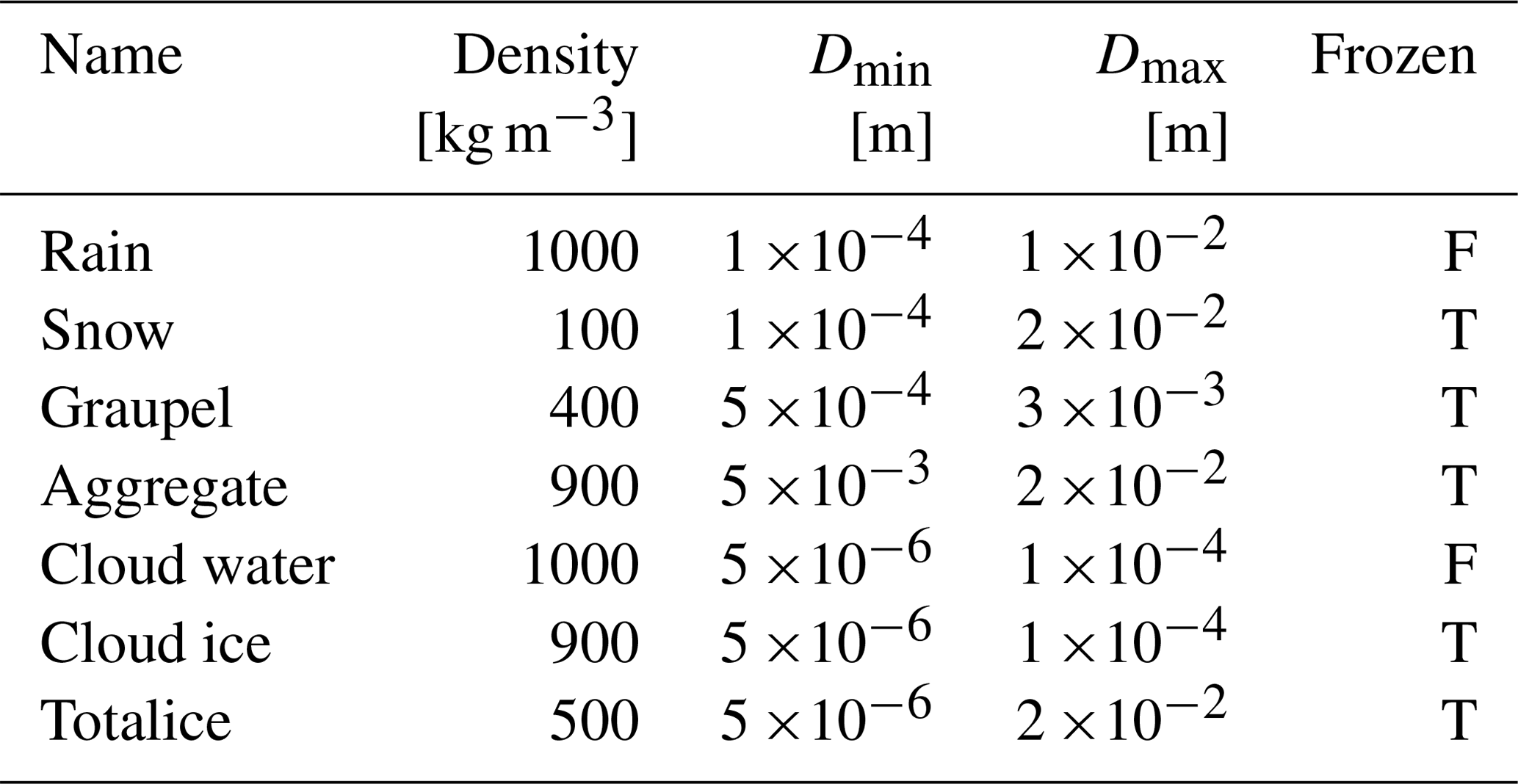
The data files contain bulk optical properties for a set of possible hydrometeor types. The default configuration of the table generator is given in Table 1, which provides five hydrometeor types representing rain, “snow” (referring to precipitating particles in stratiform cloud), “graupel” (referring to all ice particles in convective cores), cloud water, and cloud ice (referring to suspended frozen particles). This maps onto typical hydrometeor representations in global forecast models. However, the total number of hydrometeor types in RTTOV-SCATT is unlimited, and this could be used to build up more complex representations (for example, there could be different hydrometeor types for tropical and extratropical ice cloud). Each hydrometeor type is defined by a set of physical options, with the main options illustrated in Table 1; these will be described in more detail in the rest of this article. The default settings for frozen hydrometeors were obtained from a multi-dimensional parameter search in order to produce the best fits between ECMWF modelled brightness temperatures and Special Sensor Microwave Imager Sounder (SSMIS) observations (Geer, 2021b). The settings for rain and cloud water have been inherited from Bauer (2001).

Table 1 Default five-hydrometeor settings.

Acronyms for the particle size distributions (PSDs) and parameters and units of the modified gamma distribution (MGD) are defined in Sect. 3.1; all units are SI. T: true; F: false.

Each hydrometeor type needs to be associated with one of the “placeholder” types listed in Table 2. This gives the hydrometeor a descriptive name and indicates whether it is frozen or liquid. It also associates a density and size range D_min to D_max, which are mainly relevant when the Mie sphere approximation is used to compute the optical properties. If optical properties are taken from a scattering database, then the density and integration size range are instead implied by the settings for that database. Any placeholder type can be associated with any hydrometeor from the databases. The number of hydrometeor types in the lookup tables is unlimited, so the placeholder types can be re-used multiple times. Their names should not be taken too literally, such as in the use of the “snow” placeholder type with large-scale snow, and the “graupel” placeholder for frozen particles in convective clouds. The “totalice” placeholder was designed for the Met Office global model, which represents all ice particles as a single species (e.g. Doherty et al., 2007).

Table 2 Placeholder hydrometeor types.

T: true; F: false.

To save time, the table generator first calculates optical properties for the full set of possible channels (currently 136) and then it composes these channels into sets corresponding to satellite instruments (where currently 34 are represented). The list of channels and instruments is defined in a configuration file, along with the chosen hydrometeor types and physical assumptions as summarised in Table 1. One output file is then produced per instrument, containing the optical properties for each channel, tabulated as a function of water content, temperature, and hydrometeor type. The relevant grids are fixed as follows:

• for water content, 40 logarithmically spaced points from 1 $\times {\mathrm{10}}^{-\mathrm{6}}$ to 1 $\times {\mathrm{10}}^{-\mathrm{2}}$ kg m⁻³;

• for temperature, 70 points, one every Kelvin, from 204 to 273 K for frozen hydrometeors and from 234 to 303 K for liquid hydrometeors (frozen or liquid is defined according to Table 2).

The channels for any target instrument can be specified in one of two ways. The normal way is the “condensed” approach, designed for unpolarised optical properties. Instruments such as conical-scanning microwave imagers may separately measure vertical and horizontal polarisations at one frequency, but in the condensed representation this is represented as one channel in the tables. This eliminates redundancy in the data file and leaves it up to the radiative transfer model to remap the condensed set of channels onto the actual channel set of the instrument. An alternative “full” option is for use with polarised optical properties (Sect. 3.3), and in this case, the full channel set, including each distinct polarisation, is represented in the data file.

Given that over the width of a channel, bulk scattering properties vary slowly with frequency, there is no attempt to represent the exact spectral response function. Instead, channels are specified by the central frequency, and optical properties are evaluated at this exact frequency. In the case of double-sideband channels such as 183 ± 7 GHz, the calculations are done at each of the two frequencies, e.g. 174 GHz and 190 GHz, and then averaged.

Within the main RTTOV-SCATT radiative transfer code, the atmospheric profile is specified, at each model level, in terms of variables including temperature, humidity, and the sub-grid fraction and grid-box average mixing ratio of each of the hydrometeors represented in the hydrotables. The hydrometeor bulk optical properties are retrieved from the hydrotables as a function of temperature, in-cloud water content, and channel. These are then summed over the set of hydrometeors, together with the gas optical properties driven mainly by oxygen and water vapour absorption, to provide the total bulk optical properties of each layer in the model (see for example Bauer, 2001). These profiles are then input to the solver for scattering radiative transfer, which in the case of RTTOV-SCATT uses a delta-Eddington approach (for further details, see Bauer et al., 2006). Sub-grid heterogeneity of cloud fields is represented through an effective cloud fraction (Geer et al., 2009).

2.1 Single-particle optical properties

Single-particle optical properties are derived using either Mie theory, which assumes spherical particles, or from scattering databases that summarise the properties of non-spherical particle habits, which have been computed using more sophisticated methods such as the discrete dipole approximation (DDA). Currently, the Liu (2008) and ARTS (Eriksson et al., 2018) databases are available within the RTTOV-SCATT hydrotable generator.

2.1.1 Mie spheres

Optical properties of spheres are obtained using an iterative method that computes a set number of terms from the infinite Mie series, using recursion relations to evaluate the required polynomials (see for example Ulaby et al., 1981). These calculations depend only on the size parameter $x_{\mathrm{g}}=\mathit{\pi }{D}_{\mathrm{g}}/\mathit{\lambda }$ (where D_g is the diameter of the sphere and λ is the wavelength) and the complex refractive index of the material composing the sphere, $n=\sqrt{\mathit{ϵ}}$, where ϵ is the complex permittivity. For spheres composed of liquid water the permittivity models of Liebe (1989), Kneifel et al. (2014), and Rosenkranz (2015) are available. These models were evaluated in a weather forecasting context by Lonitz and Geer (2019). The Liebe model was the original option, but it is now known to have unrealistic behaviour at low temperatures and is retained only to allow backward evaluation. The Kneifel et al. and Rosenkranz models are based on recent permittivity measurements and gave better performance, with improved fit between forecast model and observations from SSMIS and other microwave imagers in areas of supercooled liquid water cloud at high latitudes. However, the Kneifel et al. model is only valid up to 500 GHz so the default and recommended option is the Rosenkranz model, which covers the full microwave and sub-millimetre range.

Frozen hydrometeors can be modelled as Mie spheres, but this is not recommended except for the smallest particles, where the scattering is in the Rayleigh regime (x_g≪1; see Sect. 3.2.4). The Mie representation of frozen hydrometeors gives excessive scattering brightness temperature depressions at lower microwave frequencies, but it generates insufficient scattering at higher frequencies, failing to reproduce the observed behaviour (Geer and Baordo, 2014). This is primarily due to excessive forward scattering from the idealised spherical particle (Sect. 4). However, the Mie capability is still used, where appropriate, to fill gaps in the scattering databases. Specifically, this supports an optional extension of the size ranges below the smallest available particles from the databases. It is also used to fill the gap below 3 GHz where the Liu (2008) database does not provide data. Frozen Mie spheres are assumed to be composed of a mixture of air and ice at the relevant density from Table 2, with pure ice assumed to have a density of 917 kg m⁻³ and air a density of 1.225 kg m⁻³. Alternatively, formulations of density as a function of particle diameter can be used, from Wilson and Ballard (1999), Jones (1995), or Brown and Francis (1995). These options were explored by Doherty et al. (2007). Permittivity of ice uses the Mätzler (2006) formulation, consistent with the ARTS scattering database (Eriksson et al., 2018). Earlier versions of the table generator followed the Mätzler and Wegmüller (1987) formulation, which differs only slightly; the option is retained in case exact backward comparison is required. The permittivity of the ice–air mixture is computed using the Fabry and Szyrmer (1999) mixing rule.

2.1.2 Mie-based melting layer

A final Mie-based option, also deprecated, is the melting layer formulation of Bauer (2001), which represents these particles as a soft ice sphere encased in a layer of water. When this option is selected, and only for nominally frozen hydrometeors, the resulting estimates of melting particle optical properties are placed in the 273 K temperature bin of the lookup tables. Melting particles can increase microwave brightness temperatures by 2 to 8 K over radiatively cold surfaces, mainly at frequencies of 37 GHz and below (Bauer, 2001). The equivalent bright band effect would be important for simulating radar reflectivity. However, DDA calculations from partially melted ice aggregates show that sphere-based models perform poorly (Johnson et al., 2016). The representation of non-spherical melting particles is a matter of ongoing research. Hence, melting particles and bright band effects are not represented by default in the hydrotable generator; this awaits the availability of realistic non-spherical melting particles in scattering databases.

2.1.3 Liu (2008) non-spherical frozen particles

Use of the Liu (2008) scattering database for non-spherical ice particles revolutionised the quality of microwave scattering simulations made by RTTOV-SCATT (Geer and Baordo, 2014). Table 3 lists the options, of which the sector snowflake was the previous default choice for snow. The other options are a dendrite snowflake and a variety of hex plates, columns, and rosettes. These habits are geometric models of ice particles which are rescaled and then discretised into a 3D grid of polarisable points for input to DDA scattering calculations. To create the database, single-particle scattering properties have been averaged over a large number of orientations in order to represent the average properties of an ensemble of totally randomly oriented particles. These averages have been tabulated at a range of particle sizes (Liu, 2008, their Table 2), frequencies from 3 to 340 GHz, and temperatures from 233.15 to 273.15 K. The database offers linear interpolation and extrapolation to a specified frequency, temperature, and size. However, this extrapolation is not used within the hydrotable generator: frequencies below 3 GHz, Mie sphere results are substituted; above 340 GHz, use of the Liu database is forbidden. For temperatures below 233.15 K the optical properties at 233.15 K are substituted. Finally, the available particle sizes define the size range over which the PSD is integrated. This integration range is shown in Table 3, with D_max being the largest size available from the database and D_min the smallest, but bounded at 100 µm on the assumption that the Field et al. (2007) PSD will be used (see Sect. 3.1).

Table 3 Particles available from the Liu (2008) and ARTS (Eriksson et al., 2018) databases.

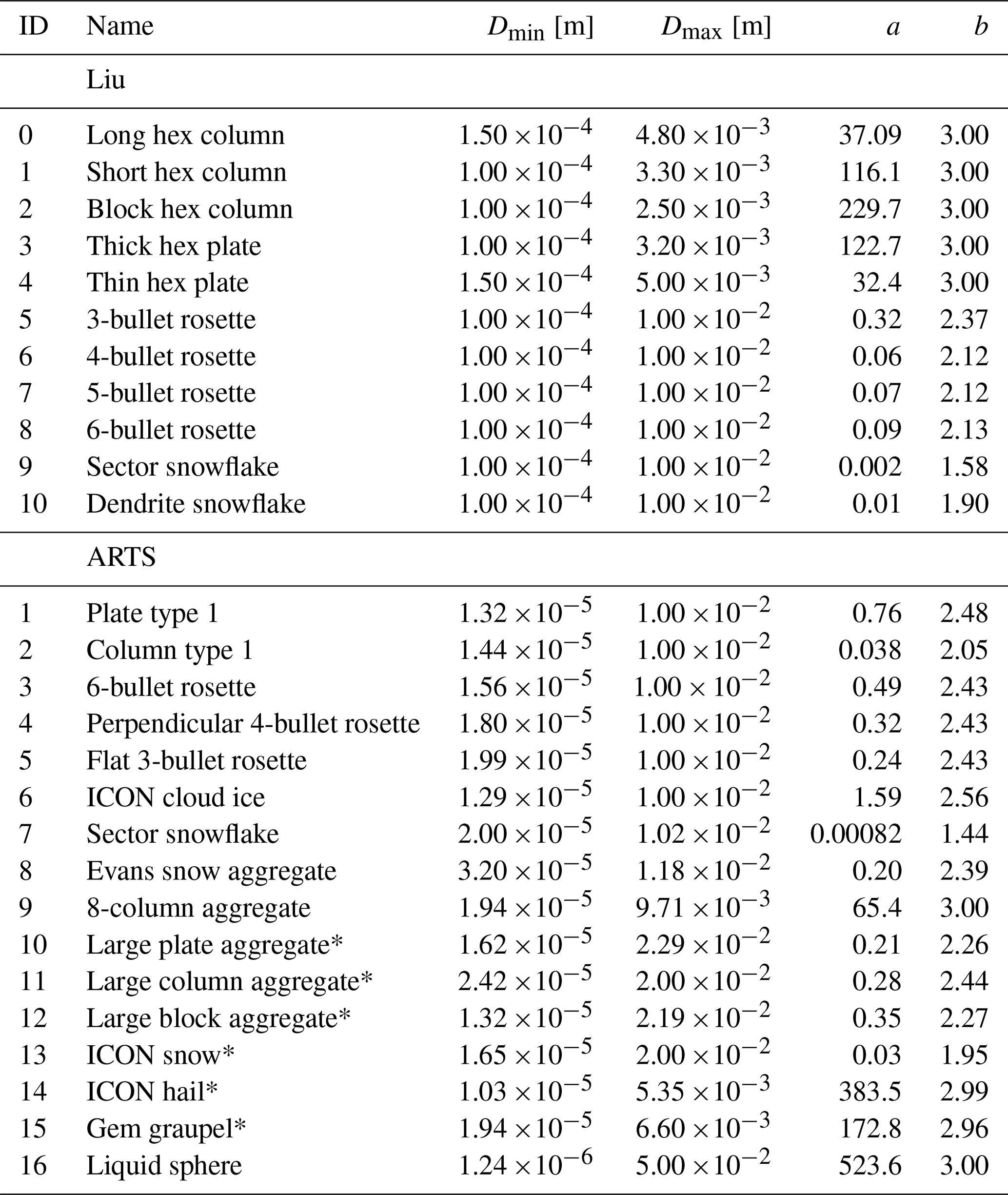
Coefficients a and b describe the mass–size relation $m=a{D}_{\mathrm{g}}^b$ and are in SI units; see the code for full numerical precision. ARTS IDs are unique to RTTOV and do not correspond to Eriksson et al. (2018); Liu IDs do correspond to Liu (2008). *ARTS standard habits with IDs from 10 to 15 are a mixture of two habits, with the small size range covered by thick plate, long column, block column, short column, gem cloud ice and 8-column aggregate respectively.

The geometric particle model also provides the link between the particle size (the geometric diameter or maximum dimension D_g) and its mass m, via the mass–size relation:

$$\begin{array}{}\text{(5)}& m=a{D}_{\mathrm{g}}^b.\end{array}$$

There is some ambiguity in the fitting of these coefficients to a particle model (Geer and Baordo, 2014). In this work, a and b coefficients appropriate to the Liu particle models have been taken from Kulie et al. (2010, their Table 1). This choice means that some particles are affected by a slightly unrealistic choice of ice density (Geer and Baordo, 2014), but these values have been retained with the aim of consistency with earlier results.

The optical properties of the Liu particles are illustrated later in Fig. 9 (or see also Kulie et al., 2010; Geer and Baordo, 2014). A limitation of the Liu database is the relatively low diversity among the bulk optical properties achievable using the different habits. For example, the 4-, 5-, and 6-bullet rosettes give similar results to the sector snowflake. Then, there is a big gap to the next-most scattering particle, the 3-bullet rosette, and another big gap to the intensely scattering hex plates and columns, which provide similar results to each other. However, these five hex particles with b=3 provide a uniquely strong bulk extinction that cannot be obtained from the ARTS database (further discussion in Sect. 4).

2.1.4 ARTS database

The ARTS scattering database (Eriksson et al., 2018) was created to support sub-millimetre as well as microwave frequencies and to provide a broader range of non-spherical ice particles, including a variety of aggregates and densely rimed particles (e.g. hail and graupel). Table 3 summarises the options available. The current default frozen particles in RTTOV-SCATT are based on ARTS particles (see Table 1).

The ARTS database provides optical properties at 34 frequencies from 1 to 886 GHz, at three temperatures (190, 230, and 270 K), and at least 34 sizes per habit. The ARTS standard habits are used here; these simplify the application of the database by ensuring a full coverage of size, temperature, and frequency. The size issue is that in the underlying database, the smallest size of aggregate habits can exceed 200 µm, so where necessary the standard habits consist of a habit mix. In these cases, the small size range is covered by a single crystal habit with a similar shape to the constituents of the aggregate (see Table 3). For example, the “large plate aggregate” habit is complemented with the “thick plate” habit. To avoid discontinuities, there is a linear transition between the two habits over a certain size range. These “mixed” standard habits are named throughout after the habit covering the main size range and contain at least 42 particle sizes. Remaining standard habits are essentially a copy of the original ones. To improve temperature coverage in the standard habits, points at 210 and 250 K are added by a second-order interpolation, in order to decrease the error by subsequent linear temperature interpolation. Finally, due to limitations in DDA, there are some gaps in the database for combinations of large size and high frequencies. In the standard habits, these gaps are filled by copying data from lower frequencies; this should be a better approximation than setting the values to zero.

When producing the RTTOV-SCATT hydrotables, the standard habit data are interpolated to the required temperature, frequency, and particle size using trilinear interpolation, with linear extrapolation also permitted up to a limit. This is used to provide values outside the available temperature range, but extrapolation in frequency or size is not used. This is because the frequency range already covers all current instruments, and the size range of the available particles from Table 3 is also used as the integration range D_min to D_max. The bulk optical properties of the ARTS particles will be explored in the rest of this work: see in particular Figs. 2, 9, 10, and 12. In most places in this work, the shortest unambiguous name (such as “ARTS plate”) is used.

2.2 Bulk optical properties

Figure 1 shows the spectral variation of bulk optical properties across the microwave and sub-millimetre frequencies. These properties have been generated from the default five-hydrometeor configuration (Table 1) for a water content l= 1 $\times {\mathrm{10}}^{-\mathrm{4}}$ kg m⁻³. A Mie sphere snow particle is also included to support discussions in Sect. 4. Rain and cloud water have broadly similar extinction per mass of particles (panel b), but because the rain particles are large enough to be in the Mie regime across most of the frequency range, they have much increased single scattering albedo (up to 0.5, panel a), asymmetry (up to 0.8, panel b), and radar reflectivity (up to 27 dBZ, panel d). Cloud water starts to depart from the Rayleigh regime above around 500 GHz, with non-zero values of the single scattering albedo and asymmetry. Moving to snow, graupel, and cloud ice, these have generally much lower extinction than the liquid particles below 100 GHz, but this reverses above around 300 GHz. Snow and graupel provide substantial scattering above around 20 GHz (SSA > 0.3), reaching to very strong scattering above 150 GHz (SSA ≃ 0.95), finally starting to decline again above 500 GHz. Cloud ice has an order of magnitude less extinction than snow and graupel at 100 GHz, and much less scattering (lower SSA) across most of the frequency range. Compared to snow and graupel, this arises mainly from the choice of PSD, which provides generally smaller particles to represent cloud ice (Sect. 3.1). Figure 1 hence shows the “spectral signatures” of hydrometeors and illustrates the utility of making measurements across the whole of the microwave and sub-millimetre range in order to characterise the physical details of cloud and precipitation particles.

Figure 1 Bulk optical properties: (a) single scattering albedo; (b) extinction; (c) asymmetry; (d) radar reflectivity for the five default hydrometeor types in RTTOV-SCATT (Table 1) plus soft Mie spheres representing snow (density 100 kg m⁻³, Field et al. (2007) tropical PSD). Computations have been done for a water content l= 1 $\times {\mathrm{10}}^{-\mathrm{4}}$ kg m⁻³ and temperatures T = 253 K for frozen particles and T = 283 K for liquid particles. Frequency steps are logarithmically distributed with 20 points per decade.

The only difference between snow and graupel in the default configuration (Table 1, Fig. 1) is the use of, respectively, an ARTS large plate aggregate and an ARTS column. The primary resulting difference is the asymmetry, with graupel giving less forward scattering between 50 and 500 GHz. This allows the graupel to generate deeper brightness temperature depressions (see Fig. 8 later). This greater “scattering” ability led to the selection of the ARTS column as a reasonable representation of convective snow (Geer, 2021b).

It is noticeable in Fig. 1 that the frozen particles have small oscillations with frequency, particularly obvious in the radar reflectivity at lower frequencies. However, these are understood² and they should not be an issue near the frequencies of typical satellite channels, since the ARTS frequencies have been chosen with this in mind (Eriksson et al., 2018).

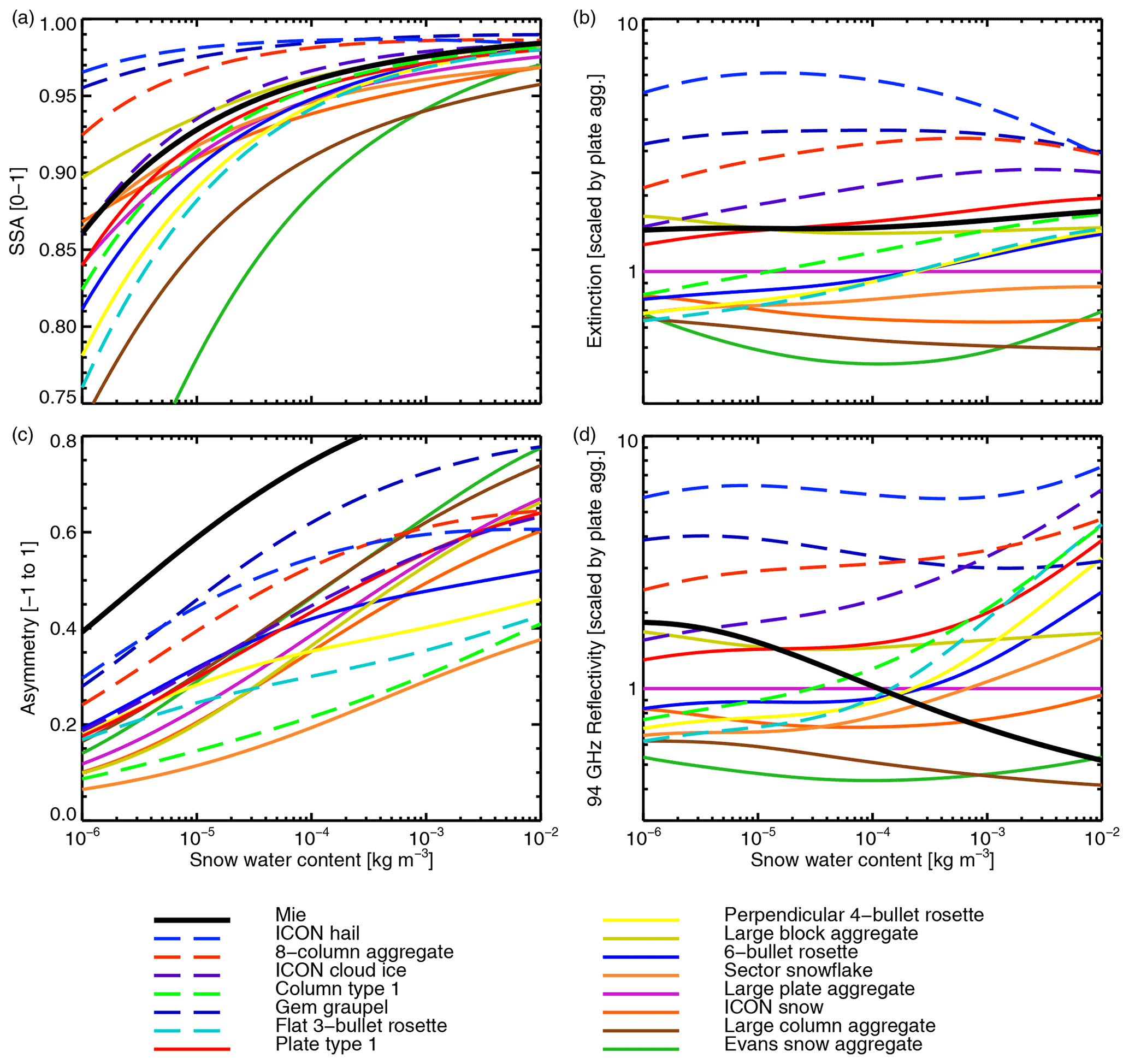
Figure 2 Bulk optical properties for the ARTS frozen particles at 183 GHz and 253 K, with the exception of panel (d) which gives the reflectivity at 94 GHz instead. The Field et al. (2007) tropical PSD has been used in all cases, with the old integration (Sect. 3.2) and a cutoff at D_min = 1 $\times {\mathrm{10}}^{-\mathrm{4}}$ m. A soft ice sphere (“Mie”) is also included, with settings as in Fig. 1. Bulk reflectivity and extinction have been normalised by those of the ARTS large plate aggregate; some lines are off scale to be able to focus on the most populated areas. The legends are in order of brightness temperature depression at 183 GHz, from most to least scattering (see Fig. 9).

Figure 2 illustrates the full range of frozen particle representations available from the ARTS database, along with the Mie sphere. The ARTS particles fall into two classes. The first is less dense particles with branched shapes including rosettes, snowflakes, and most of the aggregates. These are shown with solid lines and typically generate smaller SSA, extinction, asymmetry, and radar reflectivity. The second class is denser and more compact particles including pristine crystals, densely rimed particles (graupel and hail), and the 8-column aggregate. These are shown with dashed lines and typically generate higher values of all the optical properties. Further discussion, and comparison to the Liu (2008) particles, is made in terms of brightness temperature in Sect. 4.

2.2.1 Importance of mass–size relation

The mass–size relation (Eq. 5, specified by the a and b coefficients from Table 3) plays an important role in controlling the bulk optical properties derived from non-spherical frozen particles. In the microwave and sub-millimetre range, for a given composition (e.g. water or ice), the primary control over the single-particle optical properties is the particle's mass (e.g. Eriksson et al., 2015). Hence the mass–size relation already describes a lot about how particle size (as specified by the assumed PSD) maps onto optical properties. Further, as will be shown in Sect. 3.1, the mass–size relation also affects the shape of the PSD itself.

To summarise the available mass–size options, Fig. 3 shows those of the ARTS particles, illustrated using the effective particle density:

$$\begin{array}{}\text{(6)}& {\mathit{\rho }}_{\mathrm{e}}={\displaystyle \frac{m\left(D_{\mathrm{g}}\right)}{\left(\mathit{\pi }/\mathrm{6}\right)D_{\mathrm{g}}^{\mathrm{3}}}}\simeq {\displaystyle \frac{a{D}_{\mathrm{g}}^b}{\left(\mathit{\pi }/\mathrm{6}\right)D_{\mathrm{g}}^{\mathrm{3}}}}.\end{array}$$

This is the mass of the particle m(D_g) divided by the volume of a sphere of diameter D_g. For spherical particles, the effective density and true density are equal. The true particle mass is reported in the particle databases and is the mass of ice used in the DDA calculation; these can vary slightly from the fitted mass–size relation (see e.g. Eriksson et al., 2018, their Fig. 11). Within the hydrotable generator, it is the mass–size relation that is used to estimate the particle mass where required (primarily, in the derivation of the PSD, Sect. 3.1), but this is an approximation. In Fig. 3 the particles with b close to 3 (the hail, graupel, and 8-column aggregate) have almost constant effective density as a function of particle size. Most of the other particles have b closer to 2 and hence their effective density decreases strongly with size. Some mass–size relations generate non-physical super-dense particles when taken out of their validity range (as mentioned in Sect. 2.1.1, the assumed density of pure ice in RTTOV-SCATT is 917 kg m⁻³). This is relevant because when the PSD is fitted analytically to the water content (Eq. 10; Sect. 3.1) any super-dense region will be included. But as explored in Sect. 3.2.2 and  3.2.4 this is of little practical relevance, and even in the sub-millimetre range the bulk extinction is insensitive to ice particles smaller than 100 µm.

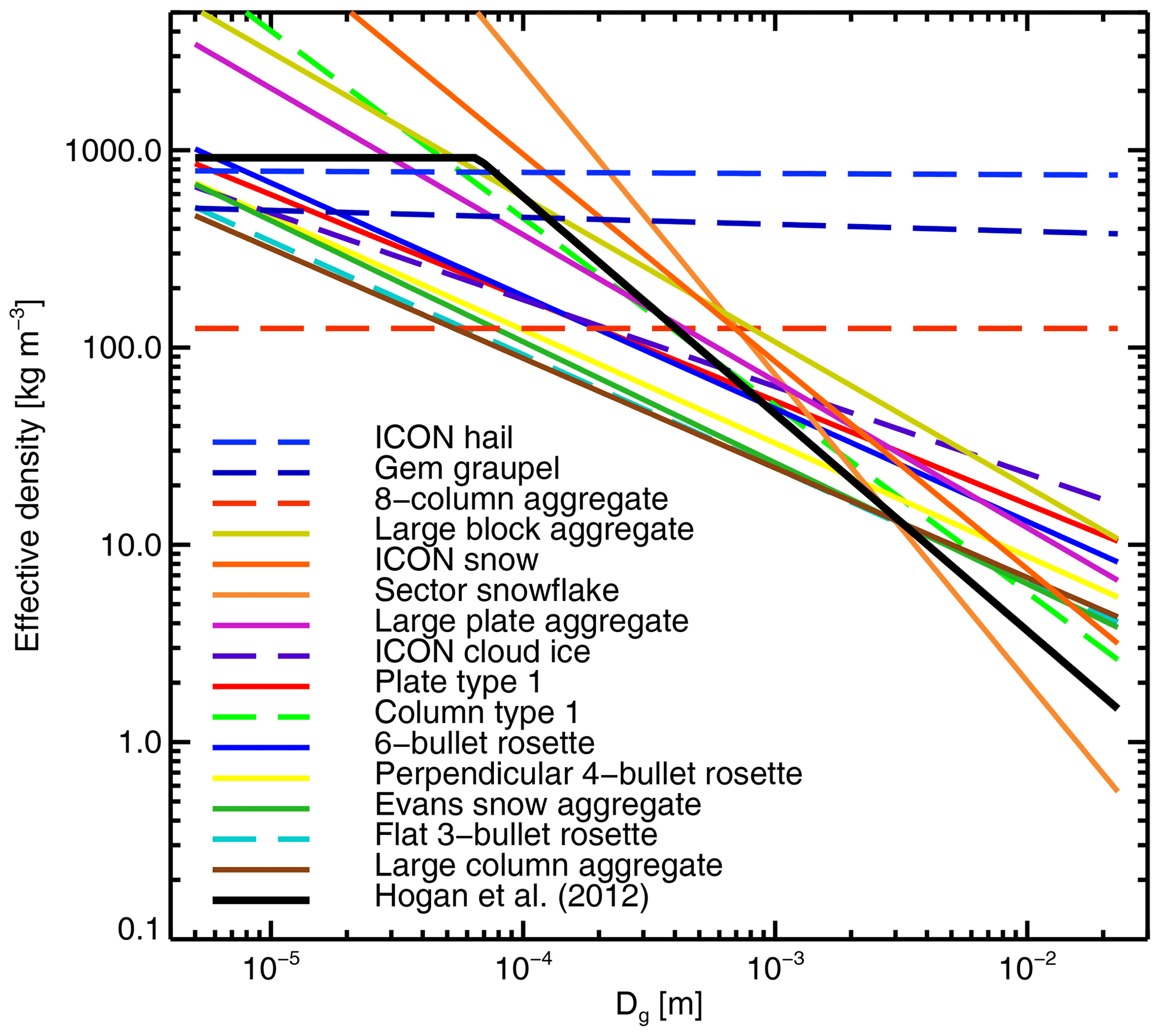
Figure 3 Effective density ρ_e implied by the mass–size relations of the particles from the ARTS database, as a function of geometric particle size (maximum dimension D_g). Also shown is the Hogan et al. (2012, their Eq. 4) restatement of the Brown and Francis (1995) mass–size relation in SI units and as a function of D_g. The ARTS mass–size relations are represented across the whole size range, even if non-physical densities may be generated, since that is how they are used in Eq. (10) (later). The legend is ordered by the effective density at 1 $\times {\mathrm{10}}^{-\mathrm{3}}$ m (with the exception of the line corresponding to Hogan et al., 2012). Figure 11 of Eriksson et al. (2018) is similar but is based on the reported particle masses, rather than the mass–size relation.

In an ideal world, users would impose their own constraints on the mass–size relation. For example, a certain mass–size relation may be assumed within the physics of the forecast model which supplies the cloud and precipitation profiles, and it may be intended to achieve microphysical consistency throughout the modelling chain. Further, there are observational constraints, and for example the Brown and Francis (1995) mass–size relation gives a good description of midlatitude stratiform ice cloud (Hogan et al., 2012); this mass–size relation is shown in Fig. 3. However, there is currently no way of decoupling the mass–size relation from the DDA particle choice in the hydrotable generator; this could only be achieved by choosing an appropriate (and probably different) database particle for each size bin – in other words, a particle ensemble approach, which is not yet supported. The Mie sphere does allow a free choice of mass–size relation (Sect. 2.1.1) but obviously brings many other drawbacks, so this is not advised. However, Fig. 3 shows that the available DDA particles span a wide range of mass–size possibilities. Further, but not shown on the figure, the dendrite particle in the Liu database (Table 3) would almost exactly match the Brown and Francis (1995) mass–size relation, for example. However, microwave radiances have their strongest sensitivity to convective snow particles, both in the tropics and midlatitudes, and the appropriate mass–size relation remains poorly known for these particles. Hence the dominant approach is to explore all potential DDA particle choices and to use the one that provides the best fit between model and observations (e.g. Geer, 2021b, and references therein). Interestingly, the best choices in that work, reflected in the default RTTOV-SCATT configuration (Table 1), seem to be particles with b around 2.0–2.4; particles with b closer to 3 seem to work poorly as a description of convective snow.

The sensitivity of optical properties to the mass–size relation is further illustrated by the sector snowflake, which is present in both ARTS and Liu (2008) databases and has almost identical optical properties as a function of particle size. However, as shown in Table 3, the a and b coefficients used with the Liu and ARTS databases are different, due to different but equally valid methodological choices in fitting those coefficients to the particle masses within the databases (see Geer and Baordo, 2014, Appendix B for further explanation). These small differences still have a significant effect on the bulk optical properties. The ARTS sector snowflake provides less scattering than the Liu equivalent, and simulations of very thick clouds using the ARTS sector snowflake and the Field et al. (2007) PSD can be up to 20 K warmer around 300 GHz (shown in Fig. 9 later). Using an identical a and b it is possible to eliminate this difference. However, it was chosen to retain the values previously used with the Liu database to ensure full back-reproducibility, but for the ARTS database to use the coefficients that are supplied with that database.

In this work, it is important to realise that when the bulk optical properties of a particle habit are discussed, this is the net result of both the physical characteristics of the individual particles and the effect of the corresponding mass–size relation on the PSD. More discussion on the importance of the mass–size relation is found in Sect. 3.1. Further explanation of how particle mass and size vary according to the microphysical choices, and how this affects the bulk scattering properties, is in Sect. 3.2.4.

3 Methods in detail

3.1 Particle size distributions

The table generator was revised at version 13.0 for a more flexible handling of PSDs and a wider set of options. One improvement in flexibility was to represent most PSDs using the modified gamma distribution (MGD):

$$\begin{array}{}\text{(7)}& n_{\mathrm{g}}\left(D_{\mathrm{g}}\right)=N_{\mathrm{0}}{D}_{\mathrm{g}}^{\mathit{\mu }}\exp \left(-\mathrm{\Lambda }{D}_{\mathrm{g}}^{\mathit{\gamma }}\right).\end{array}$$

This follows the universal framework of Petty and Huang (2011). The version of the MGD used here is based in geometric diameter or maximum dimension, D_g, consistent with the majority of available PSD formulations. n_g(D_g) is the number density of particles per unit of particle diameter, e.g. m⁻³ m⁻¹ or simply m⁻⁴. N₀, μ, Λ, and γ are the four parameters of the MGD; the units of N₀ and Λ are dependent on the units of the particle size descriptor (e.g, D_g in m) and the values of μ and γ, which are themselves dimensionless.

The kth moments of a particle size distribution are labelled M_k and are defined as

$$\begin{array}{}\text{(8)}& M_k=\underset{\mathrm{0}}{\overset{\mathrm{\infty }}{\int }}{D}_{\mathrm{g}}^k{n}_{\mathrm{g}}\left(D_{\mathrm{g}}\right)\mathrm{d}{D}_{\mathrm{g}}.\end{array}$$

The moments of the MGD can be derived analytically (Petty and Huang, 2011):

$$\begin{array}{}\text{(9)}& M_k^{\mathrm{MGD}}={\displaystyle \frac{N_{\mathrm{0}}}{\mathit{\gamma }}}{\displaystyle \frac{\mathrm{\Gamma }\left(\frac{\mathit{\mu }+k+\mathrm{1}}{\mathit{\gamma }}\right)}{{\mathrm{\Lambda }}^{\left(\mathit{\mu }+k+\mathrm{1}\right)/\mathit{\gamma }}}},\end{array}$$

where the Gamma function $\mathrm{\Gamma }\left(z\right)={\int }_{\mathrm{0}}^{\mathrm{\infty }}{x}^{z-\mathrm{1}}\exp \left(x\right)$ dx arises naturally from the integration of the MGD. This is computed in the table generator by means of a built-in Fortran function.

The PSD is fitted to the hydrometeor water content l. Where a power law mass–size relation is known, and a and b are its coefficients (Eq. 5), l is proportional to the b=kth moment of the PSD:

$$\begin{array}{}\text{(10)}& l=\underset{\mathrm{0}}{\overset{\mathrm{\infty }}{\int }}a{D}_{\mathrm{g}}^b{n}_{\mathrm{g}}\left(D_{\mathrm{g}}\right)\mathrm{d}{D}_{\mathrm{g}}=a{M}_{\mathrm{b}}.\end{array}$$

Typically all but one parameter of the MGD is prescribed and the remaining “free parameter” is adjusted to fit the hydrometeor water content. The table generator allows either N₀ or Λ to be the free parameter since the other two are less mathematically convenient. These are hence computed from Eqs. (9) and (10) as follows:

$$\begin{array}{}\text{(11)}& N_{\mathrm{0}}={\displaystyle \frac{l\mathit{\gamma }{\mathrm{\Lambda }}^p}{a\mathrm{\Gamma }\left(p\right)}}\end{array}$$

or

$$\begin{array}{}\text{(12)}& \mathrm{\Lambda }={\left({\displaystyle \frac{a{N}_{\mathrm{0}}\mathrm{\Gamma }\left(p\right)}{l\mathit{\gamma }}}\right)}^{\frac{\mathrm{1}}{p}},\end{array}$$

where $p=\left(\mathit{\mu }+b+\mathrm{1}\right)/\mathit{\gamma }$. There are a couple of issues with the analytical approach: first, any numerical integration of the PSD, such as to obtain the bulk optical properties, is necessarily done over a limited size range D_min to D_max (see Eq. 1); second, some particles with b<3 in the mass–size relation can generate non-physical super-dense small particles (Sect. 2.2.1 and Fig. 3). In the hydrotable generator these issues are partially dealt with via “renormalisation”, an empirical rescaling of the PSD described in Sect. 3.2.2.

The PSDs available in the table generator are summarised in Table 4. The Marshall and Palmer (1948, MP48) PSD is used for rain in the default configuration and is also a possibility for snow. This PSD has μ=0 and γ=1, producing what is classed as an exponential distribution; in the table generator, fixed values of N₀ are specified for liquid or frozen hydrometeors and Λ is the free parameter (see Table 4). It is optionally possible to add a temperature-dependent N₀ (Panegrossi et al., 1998, appendix), which represents the collection of smaller droplets by larger drops during sedimentation.

Marshall and Palmer (1948)Marshall and Palmer (1948)Heymsfield et al. (2013)Field et al. (2005)Field et al. (2007)McFarquhar and Heymsfield (1997)

Table 4 Available PSDs. All parameters are in SI units.

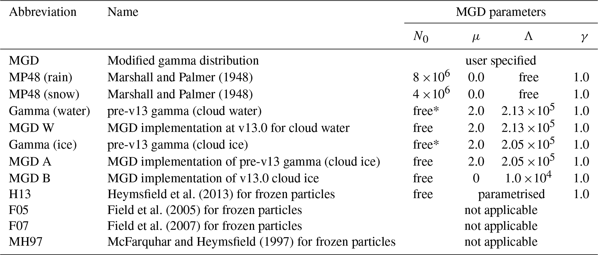
* Here, the free parameter is set using an alternative method to Eq. (11) – see text.

The “gamma” distribution, where γ=1, is often used for cloud water or cloud ice. Typically μ and Λ are prescribed and N₀ becomes the free parameter. The default configuration for cloud water follows this approach with fixed parameters that ensure cloud water particles are in the Rayleigh regime at microwave frequencies (see Table 4). The pre-v13 equivalent is retained for back-comparison purposes; this used an alternative power law fit to Eq. (11), but the resulting difference in bulk optical properties is minimal. Prior to v13.0, the gamma distribution was also used for cloud ice, also with an alternative formulation for Eq. (11). An equivalent implementation using the MGD is labelled “MGD A” and is examined later in this section. However, the default PSD for cloud ice at v13.0 (“MGD B”) was identified by parameter estimation (Geer, 2021b) and is similar to the Heymsfield et al. (2013) PSD, where its distribution becomes close to exponential (μ=0).

The Heymsfield et al. (2013, H13) cloud ice parametrisation prescribes various temperature-dependent functions for μ and Λ; these are based on aircraft measurements of ice cloud from the Arctic to the tropics. Three of the H13 configurations are available in the table generator: the stratiform (M), convective (C), or “all” (A) approach (which takes their “composite” form for Λ). The PSDs of Field et al. (2005, F05), Field et al. (2007, F07), and McFarquhar and Heymsfield (1997, MH97) are implemented outside the MGD framework and their additional details are covered in following subsections.

Figure 4a explores typical options for snow and graupel particles, using the default snow particle, the ARTS large plate aggregate. This has a mass–size relation with b=2.26, within the range of typical choices for snow and aggregates. Geer and Baordo (2014) rejected MP48 in favour of the F07 tropical (T) PSD, in order to reduce numbers of the very largest particles, which were producing too much scattering. Geer (2021b) confirmed F07 T as a reasonable choice for both large-scale and convective snow (“graupel”); it is now the default option for both. The F07 midlatitude (M) and the Field et al. (2005) PSDs are also available and could help further reduce the number of very large snow or graupel particles if needed.

Figure 4 Examples of PSDs for frozen hydrometeors available in RTTOV-SCATT, using an ARTS large plate aggregate ($m=\mathrm{0.21}{D}_{\mathrm{g}}^{\mathrm{2.26}}$ (SI)), an ice water content of 1 $\times {\mathrm{10}}^{-\mathrm{4}}$ kg m⁻³, and temperatures of 223 K (dashed) and 263 K (solid). PSDs have been split across two panels for clarity, but for reference F07 T is present in both. At 223 K, the H13 S and H13 C distributions are nearly identical below $n_{\mathrm{g}}^{\prime }\left(D_{\mathrm{g}}\right)={\mathrm{10}}^{\mathrm{7}}{\mathrm{m}}^{-\mathrm{4}}$. See Table 4 for PSD name abbreviations. PSDs have been renormalised (Sect. 3.2.2) and all have been integrated using the new approach (Sect. 3.2.1).

Figure 4b explores possible PSDs for cloud ice. The pre-v13 gamma distribution (labelled MGD A; see Table 4) made the particles very small and the simulated ice cloud was almost invisible at frequencies of 183 GHz and below. Geer (2021b) explored other options, hoping to make cloud ice more visible, as seen in observations (e.g. Doherty et al., 2007; Hong et al., 2005). A number of aircraft-based PSDs were tested (H13 S, F07 M, MH97) but all produced too much scattering, even when the particle type was chosen to generate as little scattering as possible (e.g. the ARTS large column aggregate). Figure 4 shows that these PSDs can generate significant numbers of larger particles, particularly at warmer temperatures, which must be the cause of the excess scattering. To fill the gap between the previous gamma configuration (e.g. MGD A, too few large particles) and the aircraft-based PSDs (too many large particles), new PSDs were created, inspired by the low-temperature part of H13. The configuration labelled here as MGD B (see Table 4) was ultimately chosen as the cloud ice default. Once sub-millimetre data from ICI are available, it will be seen whether this is indeed a physically reasonable choice; however, it was shown to do a reasonable job in representing observations at 183 GHz.

An issue with many ice PSDs, and particularly evident with F07 and MH97 in Fig. 4, is the presence of a “small mode” of ice particles. The aircraft measurements on which these PSDs were based were subject to probe shattering (Korolev et al., 2011) and optical effects (O'Shea et al., 2021) that, it is now thought, create a spuriously large number of small particles. Hence the small-size mode of these distributions might be non-physical. The H13 PSD is intended to be free from at least the probe shattering effect (Heymsfield et al., 2013).

3.1.1 Field-type PSDs

The Field et al. (2005, 2007) PSDs are based on a “universal” rescaled PSD Φ₂₃(x₂₃), which is a function of a non-dimensional particle size parameter $x_{\mathrm{23}}=D_{\mathrm{g}}\frac{M_{\mathrm{2}}}{M_{\mathrm{3}}}$. Here, M₂ and M₃ are the second and third moments of the PSD (Eq. 8) but any pair of moments could have been used. The universal PSD is parametrised as the sum of exponential and gamma PSDs in x₂₃ which gives the resulting PSD a characteristic population bulge in the smaller sizes (Fig. 4).

The size-based PSD is recovered by

$$\begin{array}{}\text{(13)}& n_{\mathrm{g}}\left(D_{\mathrm{g}}\right)=M_{\mathrm{2}}^{\mathrm{4}}{M}_{\mathrm{3}}^{-\mathrm{3}}{\mathrm{\Phi }}_{\mathrm{23}}\left(x_{\mathrm{23}}\right).\end{array}$$

To evaluate the PSD hence requires knowledge of M₂ and M₃, or equivalently any other pair of moments; these are obtained by an empirical relation that converts one moment to any other (e.g. Eq. 3 in Field et al., 2007). The water content l provides M_b through Eq. (10); this is first converted to M₂ and then M₂ is used to obtain M₃. The universal PSD is not itself temperature dependent, but Field et al. (2007) provide two parameterisations, one for tropical and one for midlatitude conditions. The temperature dependence arises through the empirical relation between moments, so that the F05 and F07 PSDs generate smaller particles at lower temperatures (Fig. 4).

There are some issues to consider with the Field PSDs, in addition to the small-particle mode noted before. First, the aircraft observations on which they were based did not measure particles with D_g smaller than 1 $\times {\mathrm{10}}^{-\mathrm{4}}$ m (100 µm). The universal PSD can be used to extrapolate to smaller sizes; the hydrotable generator allows this for the F05 PSD. Field et al. (2007) recommended more strongly not to extrapolate, so the table generator terminates the F07 PSD at D_min=1$\times {\mathrm{10}}^{-\mathrm{4}}$ m (Fig. 4). When the above procedure is followed to define a size-based PSD from the ice water content, it is assumed that it is valid with an integration over sizes from 100 µm to infinity. The numerical integration of the resulting n_g(D_g) and particle mass m(D_g) (following Eq. 10) should recover the original ice water content, but instead the results can be very different; this is covered in Sect. 3.2.2. The F07 T PSD has proved useful in fitting real observations, and it is vital to the default configuration of the table generator; however, users need to be aware of these complex issues.

3.1.2 McFarquhar and Heymsfield (1997) PSD

The McFarquhar and Heymsfield (1997) PSD is based on mass-equivalent diameters D_e, where

$$\begin{array}{}\text{(14)}& D_{\mathrm{e}}={\left({\displaystyle \frac{\mathrm{6}m}{\mathit{\pi }{\mathit{\rho }}_{\mathrm{ice}}}}\right)}^{\mathrm{1}/\mathrm{3}}.\end{array}$$

Here m is the mass of the particle and ρ_ice is the density of solid ice (note the table generator uses ρ_ice = 917 kg m⁻³ compared to ρ_ice = 910 kg m⁻³ in the original work). Similar to the Field PSDs, it has two modes (Fig. 4b): the first represents particles smaller than $D_{\mathrm{g}}=\mathrm{1}\times {\mathrm{10}}^{-\mathrm{4}}$ m (100 µm) using a gamma distribution in D_e. Larger particles are represented by a lognormal distribution, also in D_e; this cannot be represented in the universal MGD framework of Petty and Huang (2011). There is no hard cutoff between the distributions; rather they are summed for all D_e from 0 to ∞, observing that the two distributions do not have a big overlap. To adapt the PSDs to the specified ice water content l, the water content is first split into two parts representing the small and large particles. This is done based on an empirical relation (McFarquhar and Heymsfield, 1997, their Eq. 5). The small- and large-particle PSDs are then dependent on the partial masses (their Eqs. 3 and 4). The parameters of both PSDs are also temperature dependent (their Eqs. 7–12), producing behaviour broadly similar to Field et al. (2007, see Fig. 4b). A PSD based on geometric diameter is recovered by the conversion

$$\begin{array}{}\text{(15)}& n_{\mathrm{g}}\left(D_{\mathrm{g}}\right)={\displaystyle \frac{\mathrm{d}{D}_{\mathrm{e}}}{\mathrm{d}{D}_{\mathrm{g}}}}{n}_{\mathrm{e}}\left(D_{\mathrm{e}}\right),\end{array}$$

where $\frac{\mathrm{d}{D}_{\mathrm{e}}}{\mathrm{d}{D}_{\mathrm{g}}}$ has been evaluated numerically, and n_e(D_e) is the PSD on the mass-equivalent diameter basis.

The MH97 PSD is less sensitive to the choice of mass–size relation and hence less sensitive to variations in the particle habit (see Fig. 12). This is not, it is thought, because it is based in mass-equivalent diameter D_e, as hypothesised by Eriksson et al. (2015), but because it puts so much of the mass in the small particle mode (Ekelund et al., 2020b). As with the Field PSDs, this small-particle mode may be physically incorrect and may have been generated by probe-shattering or optical effects (Korolev et al., 2011; O'Shea et al., 2021).

3.2 Integration methods

The core of the hydrotable generator is the numerical integration over the PSD to produce the bulk optical properties, as described earlier (Eqs. 1 to 4). This section first describes the more technical aspects of the integration: numerical integration methods, renormalisation and diagnostics (Sect. 3.2.1, 3.2.2 and 3.2.3 respectively). Then Sect. 3.2.4 explores the scientific importance of the integration, illustrating the size range of particles that contribute to the bulk optical properties, and helping to explain the impact of different microphysical choices.

3.2.1 Numerical integration

In previous versions, numerical integration was done at fixed steps in particle size D_g, using a rectangle rule integration, centred on the integration point. The current version also offers an improved integration using the trapezium rule, and with log-spaced integration points in D_g to better resolve the small size ranges. The number of integration points is fixed at 100 and is the same in both methods. The integrations in Eqs. (1) to (4) use a PSD that has been renormalised to conserve integrated mass, $n_{\mathrm{g}}^{\prime }\left(D_{\mathrm{g}}\right)$; this is described in Sect. 3.2.2. For reasons to be explained, a mix of the old and new integration techniques is used in the default configuration (Table 1).

The integration of optical properties is done over the truncated range D_min to D_max. For Mie spheres, the integration range is given in Table 2. For particles from the Liu or ARTS databases, the integration size range is taken from Table 3, with two exceptions. First is that the size range can optionally be extended down to the relevant D_min from Table 2. If this option is selected, the relevant optical properties are computed using Mie theory, assuming this is valid for particles smaller than the minimum particle size (see Sect. 2.1). If the optional extension is not selected, then a minimum size D_min = 1 $\times {\mathrm{10}}^{-\mathrm{4}}$ m is applied when the F07 PSD is used with the ARTS shapes, to avoid extrapolating the PSD. Note that as described in Sect. 2.1, for the implementation of the Liu database in the hydrotable generator, the D_min = 1 $\times {\mathrm{10}}^{-\mathrm{4}}$ m constraint was imposed unilaterally in Table 3, meaning that it affects the Liu particles no matter which PSD is chosen (this behaviour is undesirable but is preserved for back-compatibility).

The numerical integration methods are illustrated in Fig. 5 using the computation of the implied water content (Eq. 16, next section). The old method is represented by the stepped red line; its grid was too coarse to resolve sharp PSD features in the small size ranges. The trapezium rule used in the new method is represented by straight lines between log-spaced integration points (indicated by the black crosses in the example with the D_min = 1 $\times {\mathrm{10}}^{-\mathrm{4}}$ m (100 µm) cutoff). The new method is a more exact representation of the integration range D_min to D_max, whereas in the old method the centred bins extended all the way down to D_g=0, indeed fractionally beyond in some cases. This means that with the old method, even if the nominal D_min was significantly above zero, the integration was still roughly representing the full size range of particles from zero to infinity. Hence if the intention were to exclude the smallest particles from the PSD, such as when the 100 µm cutoff is used with the F07 PSD, then the old integration scheme does not fully achieve this aim. The importance of this is examined in the next section.

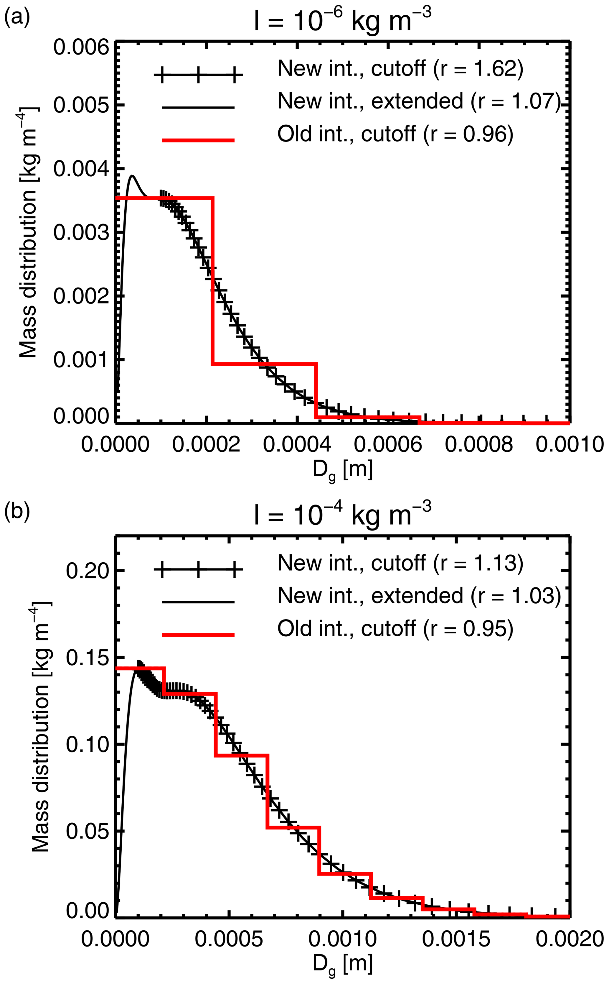
Figure 5 Numerical integration options illustrated using the reconstruction of the implied water content (Eq. 16), for the F07 T PSD with the ARTS large plate aggregate and T=223 K. The mass distribution is a(D_g)^bn_g(D_g), using the PSD before renormalisation. The specified water content is (a) l= 1 $\times {\mathrm{10}}^{-\mathrm{6}}$ kg m⁻³ and (b) l= 1 $\times {\mathrm{10}}^{-\mathrm{4}}$ kg m⁻³. The resulting renormalisation factor (r; see Sect. 3.2.2) is indicated in the legend. The integration options are the new integration with D_min = 1 $\times {\mathrm{10}}^{-\mathrm{4}}$ m (100 µm) cutoff (black crosses), the new integration extended down to D_g=5 $\times {\mathrm{10}}^{-\mathrm{6}}$ m (black line), or the old integration (red line).

3.2.2 Renormalisation

An important test of the numerical integration is whether the water content l, used to specify the PSD, can be recovered in the implied water content when the particle mass and PSD are numerically integrated across the chosen integration range D_min to D_max:

$$\begin{array}{}\text{(16)}& l_{\mathrm{implied}}=\underset{D_{\min }}{\overset{D_{\max }}{\int }}a{D}_{\mathrm{g}}^b{n}_{\mathrm{g}}\left(D_{\mathrm{g}}\right)\mathrm{d}{D}_{\mathrm{g}}.\end{array}$$

The reconstructed water content may be different due to deficiencies in the numerical integration, if the chosen particle size range omits part of the PSD, or if there are inaccuracies in the conversion from water content to PSD parameters. A renormalisation factor r can be computed:

$$\begin{array}{}\text{(17)}& r={\displaystyle \frac{l}{l_{\mathrm{implied}}}}.\end{array}$$

In order not to lose or gain mass, the PSD is renormalised as follows:

$$\begin{array}{}\text{(18)}& n_{\mathrm{g}}^{\prime }\left(D_{\mathrm{g}}\right)=r{n}_{\mathrm{g}}\left(D_{\mathrm{g}}\right).\end{array}$$

As a possible way of avoiding the renormalisation process in future, Petty and Huang (2011) have shown how an incomplete gamma function could be used to find the parameters of a truncated PSD (contrast with Eq. 12, which uses the complete gamma function).

In the current work all PSDs are renormalised using the procedure in Eqs. (16) to (18), with the exception of those shown in Fig. 5, which are not renormalised. In most cases the renormalisation is minor, with $|r-\mathrm{1}|$ less than 0.03, often much smaller. However, there are some exceptions. As shown in the figure, the F07 T PSD requires relatively large amounts of renormalisation, with $|r-\mathrm{1}|$ of 0.13 in this example (using the new integration with the 100 µm cutoff, Fig. 5b). The other main exceptions are the MGD A PSD, which has $|r-\mathrm{1}|=\mathrm{0.4}$, and the F05 PSD, which has $|r-\mathrm{1}|=\mathrm{9.1}$ at the low temperature setting where the problem is at its worst (for the same example, but not shown in Fig. 5). Since these are the PSDs with the largest number concentrations in the smallest sizes, this illustrates how the failure of Eq. (16) is typically due to a large amount of mass, and/or sharply peaked PSD features in the very smallest size ranges. This can make numerical integration difficult.

In the case of the F05 and F07 PSD, the extrapolation of the PSD below D_min = 1 $\times {\mathrm{10}}^{-\mathrm{4}}$ m exposes the question of whether to use this portion of the Field-type PSDs. Comparing panels Figure 5a and b shows that any issues are most relevant for the lowest water contents. A question is whether to truncate the F07 PSD at D_min = 1 $\times {\mathrm{10}}^{-\mathrm{4}}$ m as recommended (Field et al., 2007), or whether to allow it to extrapolate to smaller sizes. The renormalisation factors are actually largest for the new integration, with exact truncation at D_min = 1 $\times {\mathrm{10}}^{-\mathrm{4}}$ m. Renormalisations are smaller for the extended integration range and for the old integration, which effectively does not truncate the size distribution. This suggests that the reconstruction of mass using the F07 PSD may be intended to be done with an integration from 0 to infinity. In any case, the issue is that bulk scattering properties and resulting brightness temperatures generated using the F07 PSD can differ markedly depending on these details. However, the problem is worse for smaller water contents. Overall, with the F07 PSD, the least renormalisation is generated with the old integration basis (see Fig. 5) and with the 100 µm cutoff; hence even at v13.0 these are the approaches used in the default configuration of hydrometeors based on the F07 PSD. This has the advantage of retaining comparability of the results with earlier work (e.g. Geer and Baordo, 2014). But it is important to realise that the results coming from the F07 PSD are dependent on these choices.

Renormalisation is always active in the table generator, but to alert the user to any significant issues, it will throw an error if the order of magnitude of renormalisation $\left|{\log }_{\mathrm{10}}\right(r\left)\right|$ exceeds a pre-set threshold. As shown in Table 1, for hydrometeors using the MP48 and MGD PSDs, the thresholds are 0.05 or less, showing they are not much affected. For the hydrometeors using the F07 PSDs, the threshold has to be 0.5. However, the largest renormalisations are for the smallest water contents, meaning the issue does not in most cases have a significant influence on the final simulated brightness temperatures.

3.2.3 Diagnostic mode

As illustrated in this subsection, there are many complexities to the apparently simple task of numerical integration of bulk optical properties or mass, particularly since many PSDs put significant mass in the smallest size ranges, where the particles are unimportant in the microwave and sub-millimetre radiative transfer. Since it has not been possible to demonstrate or test every combination of options provided by the tool, users may wish to check the quality of the integrations for themselves. If the amount of renormalisation required is large, this is an early warning of problems, but even better is to make use of the new diagnostic mode, which writes out an additional diagnostic text file during the generation of the lookup tables. For a chosen particle ID (from Table 2), temperature, frequency, and water content, the diagnostic mode outputs the values of key parameters at each integration point: D_g, D_m(D_g), m(D_g), $N_{\mathrm{g}}^{\prime }\left(D_{\mathrm{g}}\right)$, β_e(D_g), β_s(D_g), β_b(D_g), g_single(D_g), and the “extagrand”, the numerical representation of ${\mathit{\beta }}_{\mathrm{e}}{N}_{\mathrm{g}}^{\prime }\left(D_{\mathrm{g}}\right)\mathrm{d}{D}_{\mathrm{g}}$, which is summed to create the final bulk integrated extinction. The resulting bulk values are also provided, along with the renormalisation factor r to be able to recreate N_g(D_g). The new diagnostic mode was heavily used in the development of v13.0 and in the preparation of figures for this paper.

3.2.4 Converting mass to extinction

Figure 6 illustrates the integration of extinction (Eq. 1) for frozen particles at 190.31 GHz using the F07 T PSD. The integration combines the single-particle extinction (β_e(D_g), panel a) and the PSD $\left(N_{\mathrm{g}}^{\prime }\right(D_{\mathrm{g}})$, panel b), so that each integration element gives a contribution of ${\mathit{\beta }}_{\mathrm{e}}{N}_{\mathrm{g}}^{\prime }\left(D_{\mathrm{g}}\right)\mathrm{d}{D}_{\mathrm{g}}$ to the bulk extinction (panels c and d), referred to here as the “extagrand”. The elements are logarithmic in size (the “new” integration has been used), and the size axis of the plot is also logarithmic; hence the bulk extinction is proportional to the area under the curves in panels c and d. All panels have been normalised: the extinction and the size distribution have been respectively divided and multiplied by the single-particle mass (based on Eq. 5), presenting Eq. (1) as follows:

$$\begin{array}{}\text{(19)}& {\mathit{\beta }}_{\mathrm{e}}=\underset{D_{\min }}{\overset{D_{\max }}{\int }}\underset{\text{extinction per unit mass}}{\underbrace{{\mathit{\sigma }}_{\mathrm{e}}\left(D_{\mathrm{g}}\right)/m\left(D_{\mathrm{g}}\right)}}\times \underset{\text{mass distribution}}{\underbrace{m\left(D_{\mathrm{g}}\right)n_{\mathrm{g}}^{\prime }\left(D_{\mathrm{g}}\right)}}\mathrm{d}{D}_{\mathrm{g}}.\end{array}$$

This has two aims: first to normalise quantities that would otherwise vary over more than 10 orders of magnitude; second and most importantly, to focus on the key process in the computation of bulk optical properties, which is to convert hydrometeor mass to bulk extinction. Further, to more easily compare the results with different water contents in panels c and d, the extagrand has been normalised by the respective hydrometeor water content. Panel b shows that the effect on the F07 PSD of increasing the hydrometeor water content is not just to increase the overall mass of particles, but also to significantly increase the maximum particle sizes included.

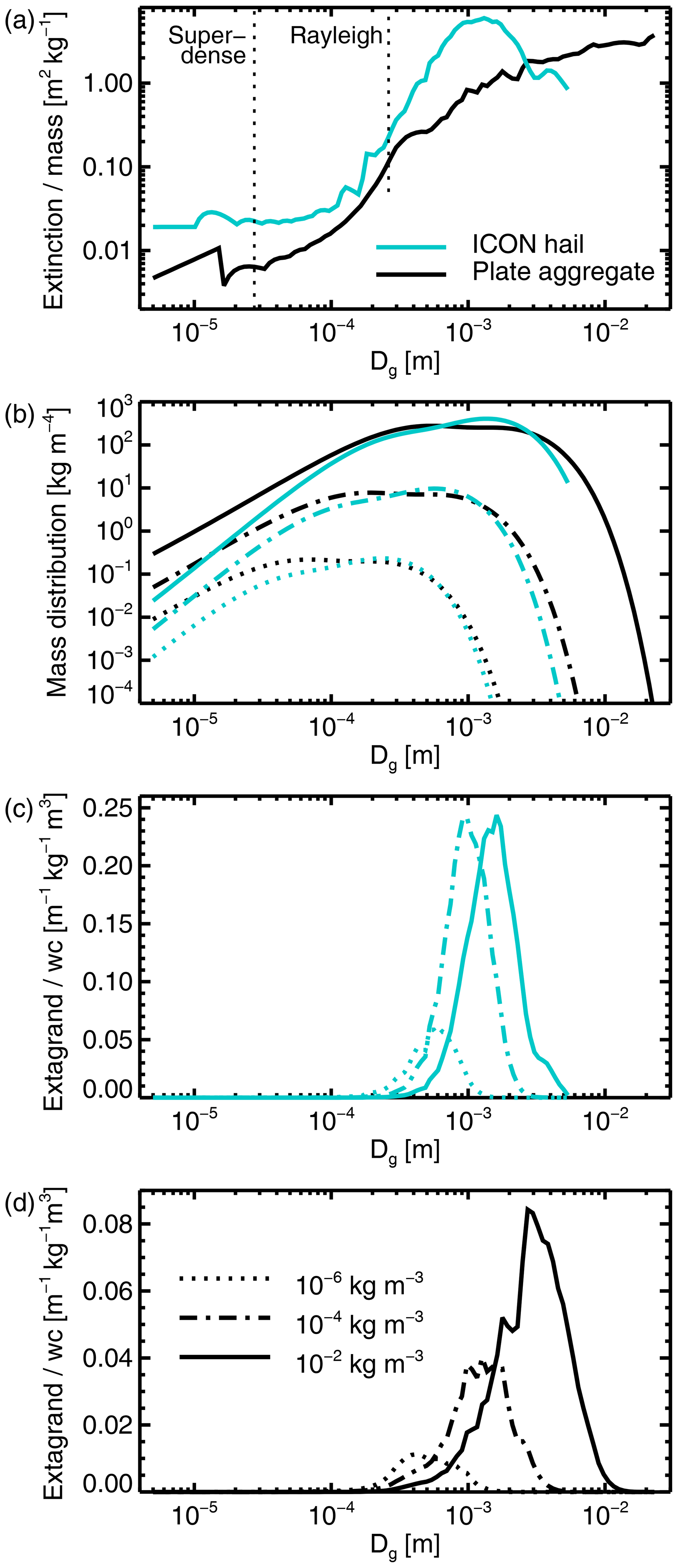
Figure 6 Integration of single-particle extinction over the PSD: (a) single-particle extinction per unit particle mass ${\mathit{\sigma }}_{\mathrm{e}}\left(D_{\mathrm{g}}\right)/m\left(D_{\mathrm{g}}\right)$; (b) mass distribution $m\left(D_{\mathrm{g}}\right)N_{\mathrm{g}}^{\prime }\left(D_{\mathrm{g}}\right)$; (c) contribution to total extinction (“extagrand”) normalised by water content ${\mathit{\sigma }}_{\mathrm{e}}\left(D_{\mathrm{g}}\right)N_{\mathrm{g}}^{\prime }\left(D_{\mathrm{g}}\right)\mathrm{d}{D}_{\mathrm{g}}/l$ for ARTS ICON hail; (d) as (c) but for ARTS plate aggregate. The F07 T PSD has been used with the “new” integration, at a temperature of 253 K and a frequency of 190.31 GHz. The extended integration range for cloud ice (down to 5 $\times {\mathrm{10}}^{-\mathrm{6}}$ m) has been used for illustrative purposes. Dotted lines on (a) correspond to, first, the largest sizes for which the plate aggregate is super-dense; second, the largest size for which Rayleigh scattering would be an appropriate model for the ICON hail particle.

For the ICON hail particle and a water content of l = 1 $\times {\mathrm{10}}^{-\mathrm{2}}$ kg m⁻³, almost all the extinction is generated by particles with D_g between 3 $\times {\mathrm{10}}^{-\mathrm{4}}$ and 5 $\times {\mathrm{10}}^{-\mathrm{3}}$ m, in other words particles with a maximum dimension of around 1 mm. This corresponds both to the peak in the mass-weighted PSD and the peak in the per-mass extinction. This peak in per-mass extinction could be called the “resonance” zone: particles with sizes that are a little larger than the wavelength give particularly large extinction even without normalisation by mass (see e.g. Petty, 2006, their Fig. 12.4). The ARTS plate aggregate is a less dense particle, and the resonance zone is found at larger particle sizes. Hence the size range contributing to the bulk extinction is between 3 $\times {\mathrm{10}}^{-\mathrm{4}}$ and 1 $\times {\mathrm{10}}^{-\mathrm{2}}$ m. The extension of the PSD to slightly larger particles (because the plate aggregate model implies different parameters in the mass–size relation) also contributes to this. But the range of particle sizes which contribute to the bulk extinction is much smaller than the range of the mass-weighted PSD. In other words, there is a significant amount of particle mass with sizes smaller than 0.3 mm that is mostly or completely “invisible”.

Within the Rayleigh scattering regime it is broadly the mass of ice, and not the particle shape, that controls the single-particle scattering properties³. For example, Fig. 12 of Eriksson et al. (2018) shows optical properties of non-spherical ice particles converging for x_e<0.5, where the size parameter $x_{\mathrm{e}}=\mathit{\pi }{D}_{\mathrm{e}}/\mathit{\lambda }$ is based on the effective (mass-equivalent) particle size, not the maximum dimension. This is a more relaxed definition of the Rayleigh regime than often suggested (x_e<0.1 is typical), but using this, the ARTS ICON hail particle departs the Rayleigh regime above D_g = 2.6 $\times {\mathrm{10}}^{-\mathrm{4}}$ m at 190 GHz. However, even in the small particle limit, the extinction per mass shown in Fig. 6a is different between the ICON hail and the plate aggregate. This is a potentially confusing aspect of using the maximum dimension D_g as the x coordinate. Because the ICON hail particle is significantly denser, it thus has higher mass for the same D_g, and hence even after normalisation by particle mass, it still has a disproportionate effect on the radiation field for the same particle size D_g. Even in the Rayleigh regime, particle morphology still needs to be taken into account when mapping from particle size D_g to particle mass; this is not a completely obvious point given that Rayleigh and Mie sphere optical properties are typically described in terms of sphere diameter, rather than mass. This also further illustrates the importance of the mass–size relation of the particle model (Eq. 5; Table 3) in determining the bulk optical properties. Interestingly, in the mass-weighted viewpoint of Fig. 6b, changing from the mass–size relation of hail (exponent b=2.99) to that of the plate aggregate (b=2.26) has only a secondary effect on the PSD shape.

A minor issue is that some particles with an exponent in the mass–size relation b<3 (Eq. 5; Table 3; Fig 3) can be “super-dense” at small sizes, in other words that the mass–size relation implies a particle density that is higher than that of solid ice. This affects the plate aggregate (but not the ICON hail) below around $D_{\mathrm{g}}=\mathrm{2.7}\times {\mathrm{10}}^{-\mathrm{5}}$ m. However, in the computation of the single-particle optical properties, whether Mie theory or DDA, particle densities are in practice not allowed to exceed those of solid ice. This could in theory result in an incorrect calculation of bulk extinction, but Fig. 6 shows that even for the smallest water contents, any issue with representing super-dense particles is irrelevant from the point of view of the optical properties, since particles as small as these are invisible. However, the treatment of small particles does affect the distribution of mass within the PSD, and hence can affect the bulk optical properties through renormalisation as explored in Sect. 3.2.2.

Figure 7 explores the frequency dependence of the range of particle sizes that are optically relevant; this is based on the ARTS ICON hail in order to show a particle which departs the Rayleigh regime at relatively low frequencies, here 10 GHz. The transition to non-Rayleigh scattering is associated with an increase of nearly an order of magnitude in the minimum particle size that contributes to the bulk optical properties (indicated by the 2.5 percentile of the integration here). However (and as also suggested by Fig. 6), the maximum particle size is more controlled by the PSD, and hence also the water content, and is less variable with frequency. This means that the size range contributing to the bulk optical properties is particularly squashed in the “resonant” region, which occurs just above the Rayleigh regime. One broad conclusion is that sophisticated models for non-spherical particle scattering are always required to correctly simulate ice hydrometeor optical properties at microwave and sub-millimetre frequencies, even for very small water contents, and even for PSDs that do not generate such large particles as the F07 T PSD (compare Fig. 4). The regions of the frequency and particle size spectrum where an approximate solution (such as Rayleigh or Mie) would be valid are those where the particles would be mostly invisible anyway. The ICON hail is the most dense available ARTS particle (Fig. 3) and would generate the most scattering from particles that are small in D_g. Hence this confirms that sub-100 µm ($D_{\mathrm{g}}<\mathrm{1}\times {\mathrm{10}}^{-\mathrm{4}}$ m) ice particles are irrelevant to the radiative transfer up to 886 GHz. Pfreundschuh et al. (2020, their Fig. 5) have shown similar results but from a point of view that excludes consideration of the PSD.

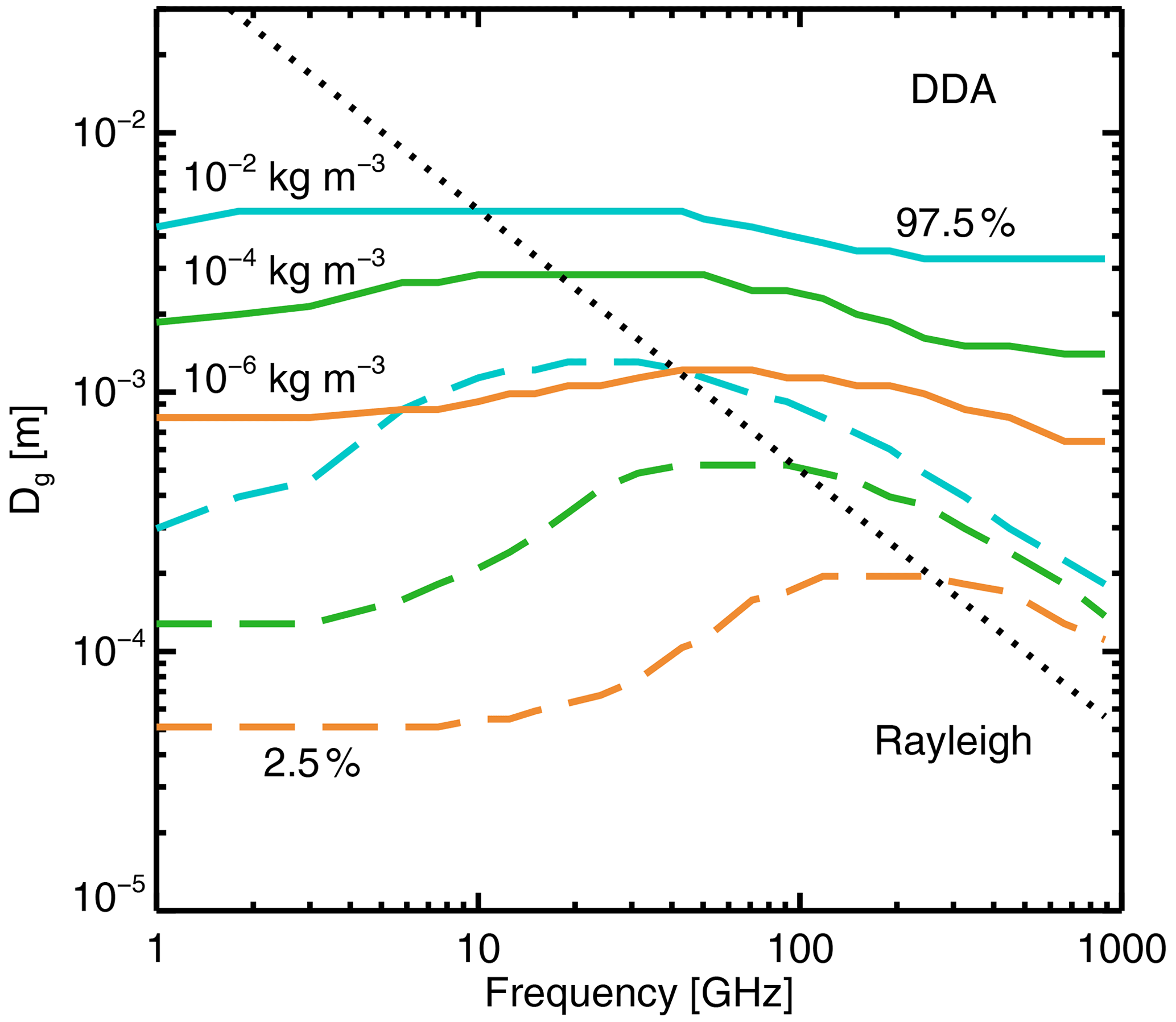
Figure 7 2.5 (dashed) and 97.5 (solid) percentiles of contributions to the integration of bulk extinction (the “extagrand” in Fig. 6c and d) for the ARTS ICON hail particle and the F07 T PSD. These are shown as a function of frequency; other aspects of the integration are as Fig. 6. Water contents are coloured as indicated in the legend. The dashed black line indicates the limit of the Rayleigh regime for this particle; above this, non-spherical optical properties must be computed using DDA or equivalent method.

Finally, an alternative viewpoint, familiar from infrared and visible cloud radiative transfer, is the cloud effective diameter. This is of less relevance to microwave radiative transfer than the particle mass, but see Appendix B for more details.

3.3 Representing preferentially oriented particles

The Liu and ARTS particles available in the hydrotable generator (and obviously the Mie sphere) represent only randomly oriented particles. However, ice hydrometeors are often preferentially oriented, as revealed by polarisation signatures in the high-frequency channels of microwave imagers (e.g. Defer et al., 2014; Gong and Wu, 2017). The ARTS database has recently been extended with a more advanced representation of particle orientation, giving particles a preferred canting angle, but retaining random orientation in azimuth (Brath et al., 2020). This generates optical properties that are fully polarised; i.e. scattering can transfer energy from one polarisation to another. To model such fully polarised optical properties would require the whole Stokes vector to be represented in the radiative transfer, but this is not available in a scalar fast model like RTTOV-SCATT. However, it is still possible to represent much of the effect of preferential orientation on microwave imager brightness temperatures, using an approximate method. This is done by scaling the bulk extinction β_e, as generated from totally randomly oriented particles, according to a polarisation ratio ρ (Barlakas et al., 2021):

$$\begin{array}{}\text{(20)}& \mathit{\rho }={\displaystyle \frac{{\mathit{\beta }}_{\text{e,H}}}{{\mathit{\beta }}_{\text{e,V}}}}={\displaystyle \frac{(\mathrm{1}+\mathit{\alpha }){\mathit{\beta }}_{\mathrm{e}}}{(\mathrm{1}-\mathit{\alpha }){\mathit{\beta }}_{\mathrm{e}}}}={\displaystyle \frac{(\mathrm{1}+\mathit{\alpha })}{(\mathrm{1}-\mathit{\alpha })}}.\end{array}$$

Here, β_e is increased by the proportion α to provide the extinction coefficient for use in horizontally (H) polarised channels β_e,H. Similarly, it is reduced by α to provide the extinction coefficient for vertically (V) polarised channels β_e,V. This description is more than just a tuning factor: αβ_e describes the bulk extinction coefficient for linear polarisation in fully polarised radiative transfer, which represents the differences in the extinction between V and H channels (Barlakas et al., 2021).

Barlakas et al. (2021) found a polarisation ratio of ρ=1.4 reproduced the observed polarisation signatures well at 166 GHz. Hence this approach is now implemented by default inside the main RTTOV-SCATT code. This operates on the fly and modifies optical properties stored in lookup tables using the standard “condensed” unpolarised representation, i.e. where optical properties are specified once per frequency, not per channel. In this approach a single polarisation ratio is applied to all frozen hydrometeors. However, RTTOV-SCATT can also accept lookup tables that are specified once per channel (the “full” representation, Sect. 2), and the table generator provides an option to generate polarised optical properties. The polarisation scaling from Eq. (20) is applied to H and V channels and is specified by an α which is a function of hydrometeor type, giving additional flexibility over the mechanism built into RTTOV-SCATT. However, it is not yet possible to specify α as a function of frequency. The polarisation ratio approach works best for conical microwave imagers with zenith angles around 50^∘ (Barlakas et al., 2021). Cross-track sounders, which have polarisation and zenith angles that vary with scan position, are not yet supported and will require further scientific development. Further, an approach for radar backscattering needs to be developed. The “full” channel representation provides a framework for future support of single-particle optical property databases based on oriented particles (e.g. Brath et al., 2020).

4 Effect of optical properties on brightness temperatures

4.1 Standardised two-stream cloud model

Although the bulk optical properties (e.g. Fig. 2) are already informative, their effect on radiation fields is both situation-dependent and a complex function of the optical properties. For example the effect of scattering on cloud-top brightness temperatures depends not just on the scattering coefficient but also the phase function, as summarised here by the asymmetry parameter. Further, even a relatively small amount of thermal emission within a cloud can substantially increase its brightness temperature compared to a purely scattering case. Hence there is a need for a standardised and simplified way to compare the cloud-top brightness temperatures arising from different choices in computing the bulk optical properties. To do this we use the two-stream solution for the radiance at the top of a uniform cloud layer taking into account both scattering and thermal emission and absorption within the cloud (Appendix C):

$$\begin{array}{}\text{(21)}& {\displaystyle }\begin{array}{rl}{I}^{\uparrow }(\mathit{\tau }=\mathrm{0})& =I_{\mathrm{0}}\left[{\displaystyle \frac{\mathrm{1}-r_{\mathrm{\infty }}^{\mathrm{2}}}{\mathrm{\Phi }}}\right]\\ & +B_{\mathrm{0}}\left[\mathrm{1}-{\displaystyle \frac{\mathrm{1}+r_{\mathrm{\infty }}\left(\exp \left(\mathrm{{\rm Y}}{\mathit{\tau }}^{*}\right)-\exp (-\mathrm{{\rm Y}}{\mathit{\tau }}^{*})\right)-r_{\mathrm{\infty }}^{\mathrm{2}}}{\mathrm{\Phi }}}\right];\end{array}\text{(22)}& {\displaystyle }\mathrm{\Phi }=\exp \left(\mathrm{{\rm Y}}{\mathit{\tau }}^{*}\right)-r_{\mathrm{\infty }}^{\mathrm{2}}\exp (-\mathrm{{\rm Y}}{\mathit{\tau }}^{*});\text{(23)}& {\displaystyle }\mathrm{{\rm Y}}=\mathrm{2}\sqrt{\mathrm{1}-{\mathit{\omega }}_{\mathrm{0}}g}\sqrt{\mathrm{1}-{\mathit{\omega }}_{\mathrm{0}}};\text{(24)}& {\displaystyle }{r}_{\mathrm{\infty }}={\displaystyle \frac{\sqrt{\mathrm{1}-{\mathit{\omega }}_{\mathrm{0}}g}-\sqrt{\mathrm{1}-{\mathit{\omega }}_{\mathrm{0}}}}{\sqrt{\mathrm{1}-{\mathit{\omega }}_{\mathrm{0}}g}+\sqrt{\mathrm{1}-{\mathit{\omega }}_{\mathrm{0}}}}};\text{(25)}& {\displaystyle }{\mathit{\tau }}^{*}=\mathit{\beta }\mathrm{\Delta }z.\end{array}$$

This solution neglects polarisation. Here, $I^{\uparrow }(\mathit{\tau }=\mathrm{0})$ is the upwelling radiance at the top of the cloud layer, which is assumed to be isotropic within each hemisphere in the two-stream approximation. The vertical coordinate is optical depth τ which is 0 at the top of the cloud and τ^* at the bottom, so τ^* is the optical thickness of the cloud. Δz is the geometric thickness of the cloud. The downwelling radiation at the top of the cloud is 0, and there is a source of upwelling radiation at the bottom of the cloud, $I^{\uparrow }\left({\mathit{\tau }}^{*}\right)=I_{\mathrm{0}}$. The upwelling radiance at the top of the cloud is given by Eq. (21) and is made up of below-cloud radiation that has been scattered or directly transmitted (the I₀ term) plus thermal emission from within the cloud, either scattered or directly transmitted to the top of the cloud (the B₀ term, where B₀ is the Planck function at the temperature of the cloud, which is uniform throughout). The additional terms Φ, Υ, and r_∞ are dependent only on the cloud's geometric thickness and the basic optical properties: the extinction β_e, the SSA ω₀, and the asymmetry parameter g from the lookup tables. The terms Φ and Υ do not have a particular geophysical interpretation, but r_∞ is the cloud-top albedo, of most relevance to solar radiation. The emitted radiation at the top of the cloud is hence a function of the three optical properties, plus the below-cloud upwelling radiation I₀, thermal emission inside the cloud B₀ (and thus the cloud temperature), and the geometric thickness of the cloud Δz.

The cloud just described is an approximate but compact description of typical situations in microwave and sub-millimetre radiative transfer. Gas absorption and emission have been neglected, and the bottom boundary of the cloud is assumed to be black, so that any radiation leaving the cloud downwards can be forgotten – for example radiation reflected from the surface is ignored. This would still be a good representation of a cloud in the upper troposphere in any part of the spectrum where water vapour or oxygen absorption blocks visibility of the surface, yet it is not a significant source of emission at the level of the cloud itself. It is also a good representation of radiative transfer over land surfaces, where the surface is mostly black. It would be trivial to add gas absorption within the cloud, and the surface-reflected term could be included but with additional complexity. But these would be a distraction from the simple standardised comparison of hydrometeor optical properties that is intended.

4.2 Overview of hydrometeor choices

Figure 8 shows the cloud-top brightness temperatures for standard two-stream clouds composed of one of the default hydrometeors from Table 1. In each case the cloud is 2 km thick and the water content $l=\mathrm{1}\times {\mathrm{10}}^{-\mathrm{3}}$ kg m⁻³. This is quite a heavy cloud of 2 kg m⁻², but this is helpful in more clearly differentiating the types of hydrometeor. The cloud temperature is 253 K if frozen (snow, graupel, or cloud ice) or 283 K if melted (rain, cloud water). A below-cloud upwelling brightness temperature of 280 K could represent a window channel over land or a lower-peaking water vapour channel (solid lines). In this case, scattering from rain generates brightness temperature depressions peaking at around 40 K, and starting above 10 GHz. Cloud water is strongly absorbing, but the situation has minimal thermal contrast, so it provides only a tiny boost to brightness temperatures. Scattering from the frozen hydrometeors is much more effective, generating depressions up to 200 K above 50 GHz for snow and graupel, and above 100 GHz for cloud ice. What gives cloud ice such different properties is not the choice of particle representation but the PSD, which selects much smaller particles (Sect. 3.1; see also Appendix B).

Figure 8 Cloud-top brightness temperatures simulated from uniform slabs composed of one of the default hydrometeor types (see legend, also Table 1) present in a 2 km thick layer with a water content of l= 1$\times {\mathrm{10}}^{-\mathrm{3}}$ kg m⁻³. The cloud temperature is 253 K if frozen (snow, graupel or cloud ice) or 283 K if melted (rain, cloud water). Upwelling brightness temperature below the cloud is 280 K (solid lines) or 100 K (dashed lines).

In Fig. 8, a below-cloud upwelling brightness temperature of 100 K (dashed lines) could represent a window channel over ocean (at lower frequencies, in horizontally polarised channels, ignoring the surface reflection) or a cirrus cloud above a very strongly scattering cloud placed lower in the atmosphere. Here, thermal emission from the rain and cloud water is the main effect above around 5 GHz. Above around 50 GHz, the frozen hydrometeors become visible, with snow and graupel generating up to 30 K brightness temperature depression even below the 100 K of upwelling radiation. The standard “graupel” configuration is a little more scattering than the “snow” particle, as intended (Geer, 2021b). In contrast, the effect of cloud ice in this scenario is to warm the brightness temperatures. Below 300 GHz, the key difference compared to graupel and snow is the relatively low SSA (Fig. 1). This warming effect of, for example, cirrus over a strongly scattering lower cloud has surprised a number of investigators (e.g. Xie et al., 2020; Barlakas et al., 2021). Where the dashed and solid lines join is where the clouds become optically thick and where below-cloud radiation becomes irrelevant. An interesting feature is that around 300 GHz to 500 GHz, snow and graupel clouds produce their lowest scattering TB depressions. Above this frequency of maximum scattering, these clouds start emitting more radiation again and brightness temperatures are higher; above 400 GHz all the frozen hydrometeor types have a warming effect. At these frequencies, SSA is high but extinction is high too (Fig. 1): a combination which must generate sufficient absorption to cause this warming.

Figure 9 shows brightness temperatures for the standardised ice or snow cloud using the F07 tropical PSD with all options from the ARTS and Liu databases; only the configuration with a below-cloud upwelling TB of 280 K is shown. The amount of brightness temperature depression from the ARTS particles roughly follows the amount of extinction in Fig. 2 and hence the progression broadly from low-density aggregates and snowflakes to dense rimed particles. The Evans snow aggregate is again the least scattering, with TB dropping only to 150 K, and again the ICON hail is the most scattering particle, dropping to 90 K. The frequency of maximum scattering varies from around 500 GHz for the Evans snow aggregate to around 200 GHz for the ICON hail. Between the extremes of light aggregate and dense hail, the ARTS database provides a good spectrum of potential scattering properties. As mentioned before, the Liu database has bigger gaps, and some of the particle shapes are almost redundant. The least-scattering Liu particle is the dendrite snowflake, but this still generates a relatively deep TB depression (as low as 130 K at 340 GHz). By contrast the ARTS database provides the column aggregate and Evans aggregate, which produce even less scattering. This provides an important new capability to reproduce cloud ice signatures. Hence the ARTS column aggregate was required in the study of Geer (2021b) and is used in the new default RTTOV-SCATT configuration (Table 1).

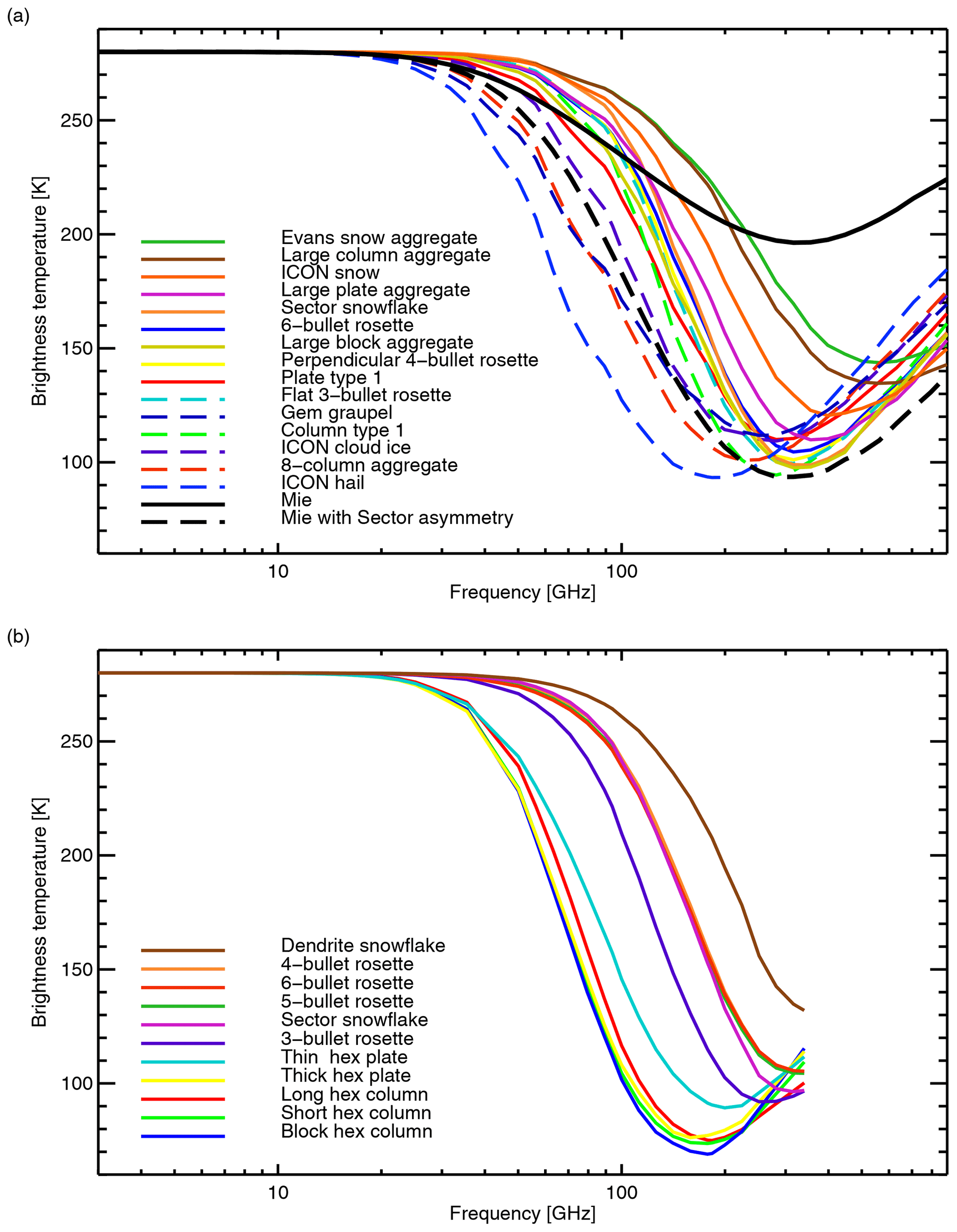
Figure 9 Cloud top upwelling brightness temperatures representing a standard ice or snow cloud at 253 K with upwelling below-cloud TB of 280 K: (a) ARTS database shapes, and a Mie snow sphere with details as Figs. 1 and 2: (b) Liu (2008) particles. In all cases the F07 tropical PSD has been used and the cloud layer is 2 km thick with a water content of l= 1 $\times {\mathrm{10}}^{-\mathrm{3}}$ kg m⁻³, as Fig. 8. The line and colour scheme for ARTS shapes is consistent with Fig. 2. Excluding the Mie sphere (black), legends in this figure are ordered by 183 GHz TB, from highest to lowest.

At the strongly scattering end in Fig. 9b, the Liu columns and thick hex plates are more strongly scattering than the ICON hail from the ARTS database, giving TBs as low as 70 K at around 180 GHz. Hence these Liu shapes continue to provide a capability that is not available from the ARTS database. However, it is interesting that the biggest variations in brightness temperature depression are in frequencies below 200 GHz. The studies of Geer and Baordo (2014) and Geer (2021b), based on SSMIS observations, have already benefitted from a spectral region of great sensitivity to particle habit and PSD. In these studies, the most strongly scattering particle models, those which generate deep TB depressions even at 50 GHz, have been decisively rejected, at least as a means of representing the effect of snow on TBs representing a global model grid box on the 10–100 km scale.

Now is a good point to tidy up some loose ends from Geer and Baordo (2014), who rejected the Mie soft sphere as a viable model for snow particles at microwave frequencies. This was partly based on the excessive scattering below 100 GHz, in common with the dense non-spherical particles just described. However, the soft sphere also provided insufficient TB depressions at 183 GHz; it is very clear in Fig. 9a that it is an outlier compared to more-realistic non-spherical particle models. Geer and Baordo suggested that the primary problem of the soft sphere was not its overall level of extinction or scattering, but its unusually high asymmetry parameter, and hence stronger forward scattering (see Fig. 2: at 183 GHz and l= 1 $\times {\mathrm{10}}^{-\mathrm{3}}$ kg m⁻³, the asymmetry of the soft sphere is around 0.9, compared to around 0.3 for the ARTS sector snowflake). The hypothesis was not confirmed in the study, but the standardised cloud model helps to clarify. The black dashed line in Fig. 9a shows TBs generated using the Mie bulk optical properties but with the asymmetry parameter from the ARTS sector snowflake. This hybrid particle gives a TB signature that is similar in some parts to the ARTS 8-column aggregate, making it indistinguishable from the DDA-based non-spherical particles. Hence it is the strong forward asymmetry of the Mie soft sphere that makes the difference. This result shows the utility of the standardised cloud model for assessing bulk optical properties, and the importance of the asymmetry parameter (and more broadly the phase function) in determining the brightness temperature.

4.3 Optical behaviour of frozen hydrometeors in the microwave and sub-millimetre

Figure 10 explores the sensitivity of the brightness temperatures to the cloud thickness, showing clouds of 0.2 km and 10 km geometric depth (respectively 0.2 and 10.0 kg m⁻² integrated water content, respectively), and roughly representing frontal ice clouds compared to tropical deep convection. These can also be compared to Fig. 9a with the “standard” cloud of 2 kg m⁻². For the thin clouds, the deepest scattering TB depressions are at high frequencies, for example at 600 GHz for the large block aggregate. There is reasonable sensitivity to particle shape across all the higher frequencies, with a 50 K difference between the most- and least-scattering shapes. For the thick clouds, TB depressions move to lower frequencies and get deeper still, with the ICON hail giving at TB of 50 K at 100 GHz. At these mid-frequencies, the sensitivity to the particle shape of thick clouds is very strong, with around 150 K difference between the most and least-scattering particle. This frequency of maximum TB depression is not fixed, however, and increases to 350 GHz for the same particle in the thin-cloud case. Conserving the integrated water content, but changing the water content by an order of magnitude in either direction (e.g. l= 1 $\times {\mathrm{10}}^{-\mathrm{2}}$ kg m⁻³ or 1 $\times {\mathrm{10}}^{-\mathrm{4}}$ kg m⁻³, not shown), the broad layout of these figures remains similar. Three interesting things appear above the frequency of maximum TB depression: first, the brightness temperatures start to become less sensitive to particle shape (and hence also particle size), which is particularly evident in the clustering in Fig. 10b; second, there is an inversion in the ordering of scattering, with the dense particles (pristine crystals, hail and graupel) generally giving slightly warmer brightness temperatures than the less-dense aggregates and rosettes; third, sensitivity to the integrated water content starts to disappear, with the thin cloud giving similar brightness temperatures at 900 GHz to the thick cloud.

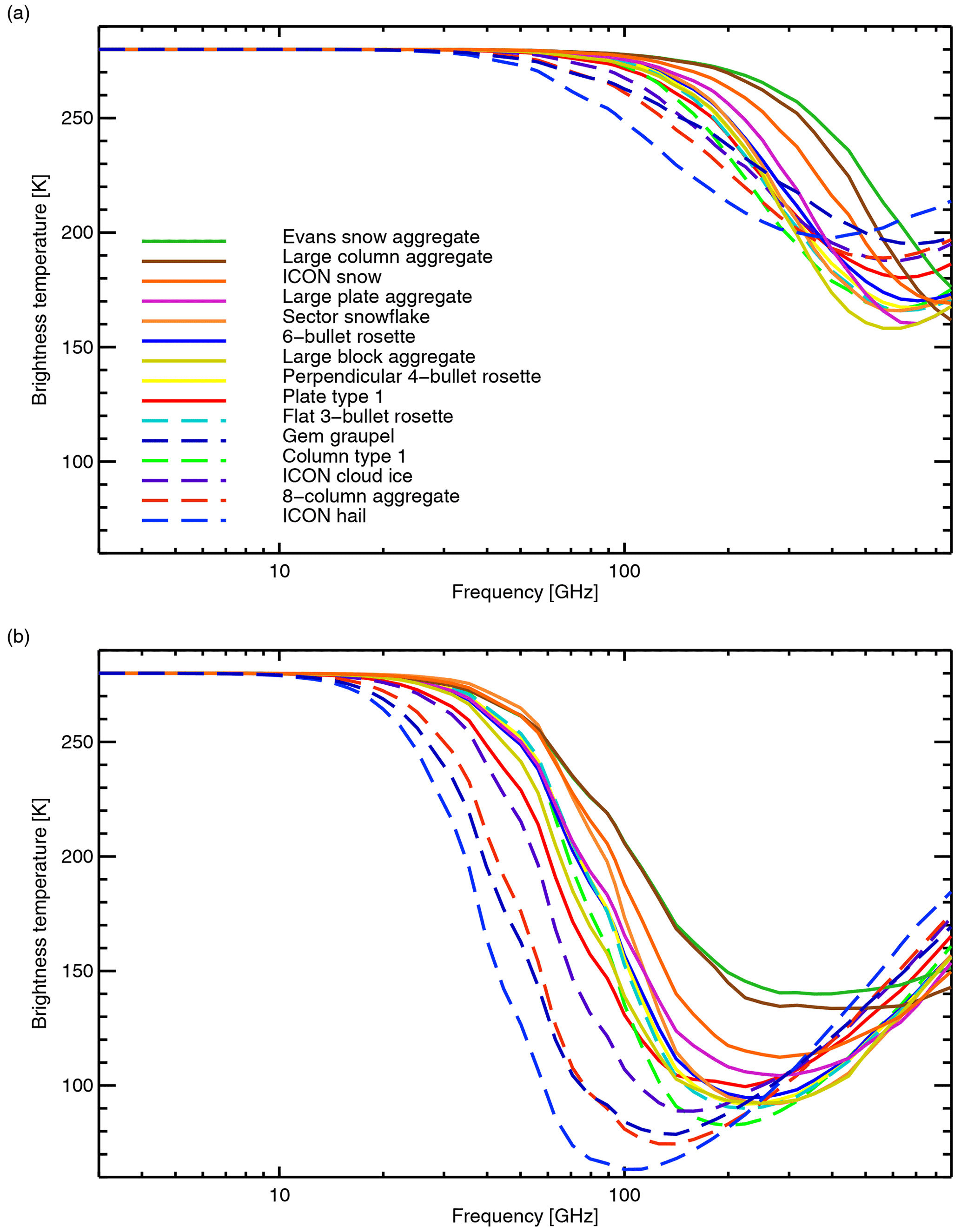
Figure 10 Brightness temperatures from a standard snow or ice cloud; details as Fig. 9a, including a fixed water content of l= 1 $\times {\mathrm{10}}^{-\mathrm{3}}$ kg m⁻³, but with a cloud geometric thickness of (a) 0.2 km; (b) 10 km.

To further explain the transition in cloud optical properties as the frequency increases, we can return to Eq. (21). The cloud brightness temperature results from two terms: radiation transmitted by the cloud and radiation emitted by the cloud. The terms in square brackets multiplying I₀ and B₀ are hence the transmittance and the emissivity of that cloud. These terms are shown in Fig. 11 along with the total brightness temperature. This is based on the strongly scattering ARTS ICON hail particle with the F07 T PSD, in order to show as much as possible of the transition within the available frequency range. The transmittance of the 2 km thick cloud goes to zero towards 1000 GHz; in other words radiation from below can no longer pass through the cloud. However, the total brightness temperature bottoms out at around 100 K, rather than dropping to zero, due to increasing thermal emission from within the cloud. As illustrated in Fig. 1, albeit with a different particle type, the single scattering albedo never reaches 1 (which would imply complete scattering or zero thermal emission); instead it reaches a maximum somewhere around 500 GHz and starts to drop off at higher frequencies. This, along with the steady increase in overall extinction, must contribute to the continuous increase in thermal emission as the frequency increases. The clouds do not need to be optically thick to show this effect; Fig. 11 also shows the 0.2 km cloud, which even at 884 GHz has a transmittance of 0.5, but still has sufficient thermal emission to contribute significantly to the brightness temperature. Hence the spectral region around 500 GHz seems to be the turnaround point beyond which cloud optical behaviours tend towards those more familiar from the infrared, with increasing optical thickness, and cloud emission becoming the dominant optical process.

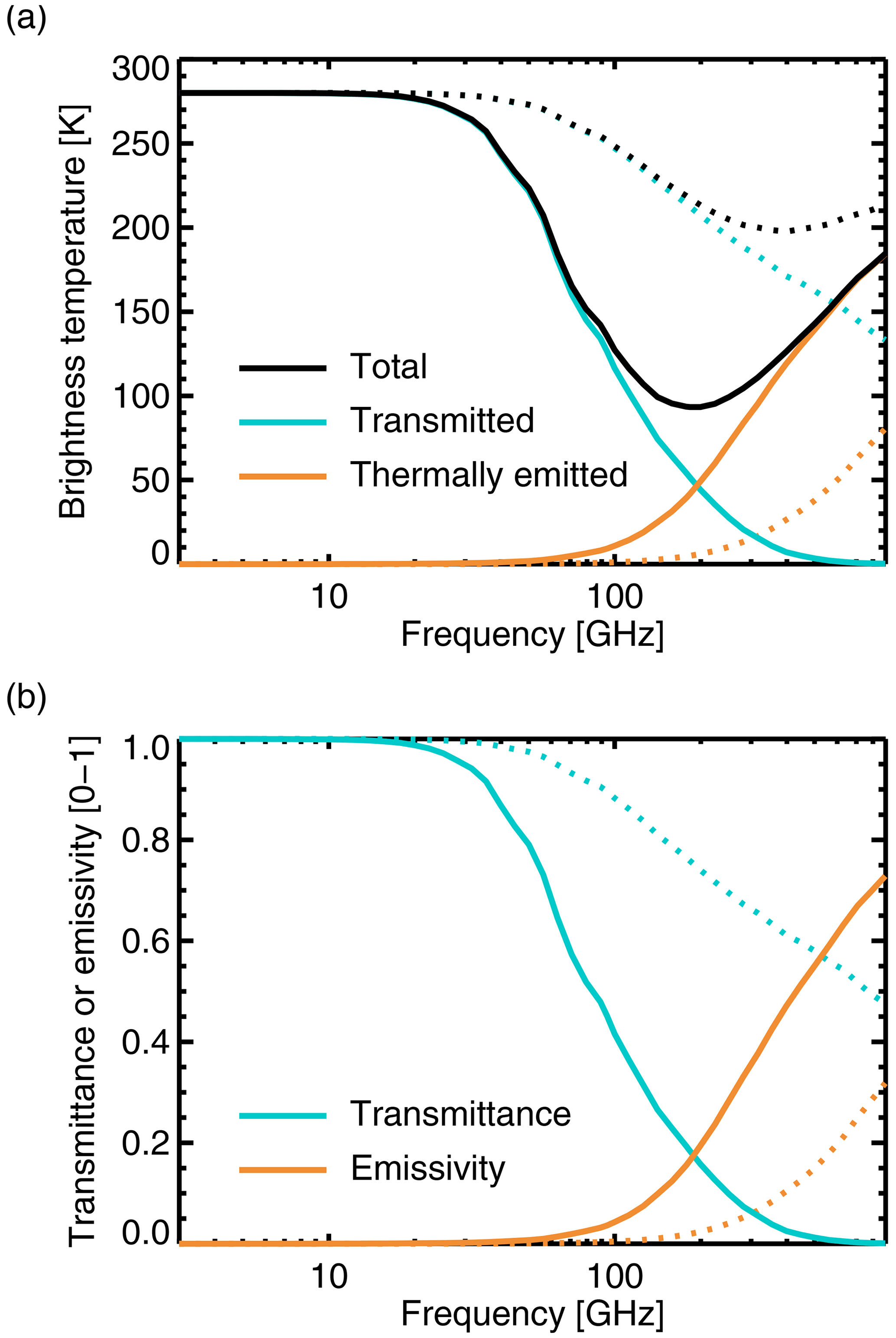
Figure 11 (a) Brightness temperatures, divided into the transmitted and emitted parts of Eq. (21); (b) transmittance and emissivity of the same cloud, i.e. the terms in square brackets in Eq. (21). This is a standard cloud with a thickness of 2 km (solid) or 0.2 km (dotted), with the ARTS ICON hail particle, F07 T PSD, and other settings as seen in Figs. 9 and 10.

4.4 Sensitivity to PSD

Figure 12 explores the sensitivity to alternative PSDs, with the representation of ice cloud in mind. The Heymsfield et al. (2013) PSD (Fig. 12a) provides quite similar results to F07. Although the order of scattering varies slightly in the detail, compared to Fig. 9a, the main features of the ARTS particles are preserved. MH97 generates a more compact spread of brightness temperatures across the ARTS particles, but it does not much change the overall order of scattering. The Evans snow aggregate, for example, is still the least scattering of the particles. This compact spread is attributed to the MH97 PSD putting a relatively high proportion of particles in the smaller size ranges (Ekelund et al., 2020b) and hence keeping more of the particles in the Rayleigh regime. However, the bunching of the different particle models still occurs above 500 GHz, suggesting this is not strongly affected by the particle size. Hence this supports a fairly universal transition towards an emission-dominated, optically thick regime above 1000 GHz, where sensitivity to particle size and shape appears to become smaller.

Figure 12 Brightness temperatures from a standard snow or ice cloud; details as Fig. 9a but exploring different PSDs: (a) Heymsfield et al. (2013, H13); (b) McFarquhar and Heymsfield (1997, MH97).

5 Conclusion

This work has summarised the process of generating bulk hydrometeor optical properties based on physical assumptions about the sizes, masses, habits, and orientations of cloud and precipitation particles. It documents the hydrotable generator for microwave and sub-millimetre scattering radiative transfer in version 13.0 of RTTOV (Radiative Transfer for TOVS, Saunders et al., 2018, 2020), a widely used satellite simulator, hopefully with relevance to the users of many similar tools. The work has overviewed the bulk optical properties and brightness temperatures generated by Mie spheres and two databases of non-spherical ice particles (Liu, 2008; Eriksson et al., 2018).

A focus has been the existing and newly supported particle size distributions (e.g. McFarquhar and Heymsfield, 1997; Petty and Huang, 2011; Heymsfield et al., 2013) and the core process of numerical integration across them. This process maps from a chosen particle size distribution and particle model, through to individual particle masses and other physical properties, and finally through to bulk optical properties. This process has a number of issues. For example, very small (< 100 µm) particles are invisible at these frequencies but can affect the bulk optical properties through renormalisation adjustments to the PSD, relating back to the underlying question of whether current PSDs do a good job of representing small particles (Korolev et al., 2011; O'Shea et al., 2021). Furthermore, the effect of small differences in the particle mass–size relation has been highlighted in the results using the ARTS and Liu sector snowflakes, which have exactly the same single-particle optical properties but generate significantly different brightness temperatures due to slightly different mass–size relations.

To illustrate the available options, a standardised homogeneous layer cloud was proposed. This is based on a simple two-stream analytical solution and converts the bulk optical properties into brightness temperatures, which are easier to interpret. In particular this resolves the trade-offs between the absolute level of scattering (the scattering coefficient) and the asymmetry parameter (summarising the shape of the scattering phase function) in the amount of brightness temperature depression that is generated. A further aspect of the standardised homogeneous layer cloud is that it illustrates the balance between radiation coming into the cloud from below, which may be scattered or absorbed, versus thermal emission from the hydrometeors themselves. This is particularly important for frozen particles above 200 GHz where, as we have shown, the cloud optical properties start to move towards an emission-dominated, optically thick regime that is much less sensitive to particle size and shape, a regime more familiar from the behaviour of clouds in the infrared.

The standardised cloud helps further investigate the soft Mie sphere as a representation of ice particles. This has unusually strong forward scattering (high asymmetry) compared to most non-spherical particle models representing the same ice mass (e.g. Eriksson et al., 2015, their Fig. 3). This unusually strong asymmetry is also found in the bulk scattering properties. The standardised cloud model shows that the spherical model cannot generate sufficient brightness temperature depressions at higher frequencies. It generates a “scattering spectrum” that is very different to any more physically reasonable model. Just by replacing the asymmetry of the soft Mie sphere with that from a non-spherical model, it becomes a much more plausible representation falling within the range of non-spherical models. This is further proof, if any is needed, of the problems with the Mie sphere representation of snow; Kuo et al. (2016) have made a very similar point. Only within the Rayleigh regime do spherical and non-spherical particles generate similar optical properties as a function of the particle mass. However, even at 10 GHz a significant fraction of ice particles can be outside the Rayleigh regime (Fig. 7); hence there really is no alternative to taking account of the microphysical characteristics of realistic non-spherical ice particles when simulating observations in the microwave and sub-millimetre regions.

An underlying assumption in this work (and many others that follow the same approach) is that clouds can be represented using a single particle shape model to cover all instances of a highly heterogeneous class of particles like snow – a “one shape fits all” approach. An important aspect of this approach is that the particle shape model defines the mass–size relation; this affects the bulk scattering properties both by its influence on the shape of the PSD and simply by defining the mapping between maximum dimension D_g and the particle mass, which means that particles of nominally the same size can generate very different single-particle optical properties. This applies even within the Rayleigh regime. The use of mass-equivalent diameter D_e could remove the latter issue (e.g. Eriksson et al., 2015), but this is of less practical relevance as long as the PSDs which are used to map from water content to particle size (and hence mass) are defined in terms of maximum dimension D_g. A more physically based approach would be to consider an ensemble of particle habits (e.g. Kulie et al., 2010; Baran et al., 2011) and might impose a mass–size relation thought to be an appropriate description of certain hydrometeors, such as midlatitude stratiform ice clouds (e.g. Brown and Francis, 1995; Hogan et al., 2012). However, RTTOV has the job of modelling satellite observations with reasonable accuracy across the entire globe; microwave observations are strongly sensitive to many different cloud regimes and particularly to those such as deep convection, where even basic details of the microphysics remain poorly known. Forecast models are currently incapable of representing the full range of microphysical parameters needed to constrain the hydrometeor optical properties; therefore simplification and generalisation is unavoidable, with parameter estimation being the ideal method for identifying the best microphysical assumptions (Geer, 2021b, with an appropriate Bayesian framework this could incorporate prior expert microphysical knowledge, such as the realism of particle habits, PSDs, and mass–size relations). In the event that a much richer microphysical representation is required, RTTOV-SCATT allows an unlimited number of hydrometeor categories that could be used to represent almost any level of microphysical complexity. Hence the tools are already available, but the underlying issue is whether it is possible to appropriately specify this complex microphysics.

There are many ways to further improve the representation of bulk scattering from hydrometeors, most of them applicable generally:

• RTTOV (as well as many other codes) uses a different mechanism and different physical assumptions for the optical properties of clouds in the IR and solar regions. A major future development should be to produce optical properties from the microwave to the UV using the same approaches as much as possible; this requires non-spherical scattering databases to be expanded to cover the whole range, a process that is only starting (e.g. Yang et al., 2013; Baran et al., 2014; Ding et al., 2017; Baran et al., 2018).

• More work is needed to unpick the tight coupling between the particle shape model, mass–size relation, and the particle size distribution. Better ways of mapping bulk hydrometeor mass to particle ensembles would be very welcome.

• More work needs to be done to standardise and/or interface the physical assumptions, such as shape, PSD, and mass–size relation, with assumptions made in atmospheric models. This would particularly support efforts to learn better physical models of cloud and precipitation, directly from observations (e.g. Schneider et al., 2017; Geer, 2021a).

• A global effort is ongoing to standardise and package many of the different scattering databases that are becoming available (see Kneifel et al., 2018); once complete, interfaces will be added to allow the user a much broader choice of particle models. This would allow the use of non-spherical oriented raindrops, for example (e.g. Ekelund et al., 2020a).

• Current PSDs have significant limitations, such as the small-particle bulge that is now thought to be unphysical (Korolev et al., 2011; O'Shea et al., 2021). Even modern PSDs based on large amounts of aircraft data, like Heymsfield et al. (2013), provide large numbers of large (centimetre-sized) particles, so in RTTOV-SCATT they do not provide a good representation of the “cloud ice” category in global models (Geer, 2021b). As with the simple exponential PSD now used as the default for cloud ice, it may in some cases be better to infer PSDs through parameter estimation, using the parameters of the standardised modified gamma distribution (MGD, Petty and Huang, 2011).

• A representation of non-spherical melting hydrometeors (e.g. Johnson et al., 2016; Leinonen and von Lerber, 2018) needs to be included. This will be particularly important for simulating radar backscatter in the melting layer (the bright band). It would also improve brightness temperature simulations, which may otherwise be too low in channels and situations sensitive to the melting layer, possibly by up to 8 K (Bauer, 2001).

This survey has also revealed a few issues more specific to the RTTOV hydrotable generator:

• Since mass (or the mass-equivalent diameter D_e, Eq. 14) is a much stronger predictor of microwave and sub-millimetre optical properties than the geometric diameter (equivalently maximum dimension) D_g, this could be a better basis with which to represent PSDs, to compare particle choices, and to do numerical integration. However, there is some tension between this and the aim to do things consistently across all frequencies (and consistently with forecast models) where sometimes the geometric size of the particles is more important. Further investigation is necessary.

• The lowest temperature bin, at 203 K, is at least 20 K higher than the lowest tropospheric temperatures. Hence, in a future version, it is necessary to extend the lower temperature range of frozen particles permitted by the table generator. Note that, although the lowest temperature point in the ARTS database is 190 K, Eriksson et al. (2018) showed that extrapolation would be reasonably accurate down to 150 K.

• The default representation of rain has not been updated since Bauer (2001); apart from the aforementioned points on shape and orientation, it is worth examining how well the rain PSD is represented, and potentially updating this.

• The code is operated offline, with a lookup table approach, but it is fast enough to be operated online within the radiative transfer code, especially as weather forecasting systems get more capable (e.g. English et al., 2020). This will be an aim of future development work.

To summarise, the future evolution of the code may be towards online operation, so that parameters of the PSD and even particle shape can be estimated directly from the observations, rather than prescribed in a “one shape fits all” approach.

Appendix A: Radar reflectivity

The radar reflectivity factor is computed as a scaling of the computed backscatter β_b from Eq. (3),

$$\begin{array}{}\text{(A1)}& Z={\displaystyle \frac{{\mathrm{10}}^{\mathrm{18}}}{z_{\mathrm{0}}}}{\mathit{\beta }}_{\mathrm{b}},\end{array}$$

where the factor 10¹⁸ converts from SI to the more typical unit of mm⁶ m⁻³ and z₀ is a frequency-dependent constant that comes from the standard definition of the radar reflectivity factor (e.g. Petty, 2006). The radar reflectivity factor is the sixth moment of a notional distribution of liquid spheres that would produce the same backscatter, assuming the Rayleigh scattering approximation:

$$\begin{array}{}\text{(A2)}& {\mathit{\beta }}_{\mathrm{b}}^{\mathrm{Rayleigh}}=\underset{z_{\mathrm{0}}}{\underbrace{{\displaystyle \frac{{\mathit{\pi }}^{\mathrm{6}}}{{\mathit{\lambda }}^{\mathrm{4}}}}{\left|{\displaystyle \frac{{\mathit{ϵ}}_{\mathrm{water}}-\mathrm{1}}{{\mathit{ϵ}}_{\mathrm{water}}+\mathrm{2}}}\right|}^{\mathrm{2}}}}\underset{M_{\mathrm{6}}=Z}{\underbrace{\underset{\mathrm{0}}{\overset{\mathrm{\infty }}{\int }}{D}_{\mathrm{g}}^{\mathrm{6}}{n}_{\mathrm{g}}\left(D_{\mathrm{g}}\right)\mathrm{d}{D}_{\mathrm{g}}}}=z_{\mathrm{0}}Z.\end{array}$$

Hence this defines the constant z₀, with the backscatter cross section of the notional liquid spheres given by the Rayleigh scattering approximation (${\mathit{\sigma }}_{\mathrm{b}}\left(D_{\mathrm{g}}\right)=z_{\mathrm{0}}{D}_{\mathrm{g}}^{\mathrm{6}}$). ϵ_water is the complex permittivity of liquid water at the radar frequency, at an assumed temperature of 273 K, and λ is the corresponding wavelength. The reflectivity constant z₀ is calculated within the hydrotable generator, using the chosen settings, and hence is dependent on the chosen liquid water permittivity model (see Sect. 2.1). Therefore it is worth making sure that the reflectivity definition used in RTTOV is consistent with the definition used for the target satellite instrument; future work could try to make sure that RTTOV sets these assumptions automatically.

Appendix B: Relevance of effective diameter

As explained in the main text, for a particular composition (water or ice) it is the particle mass that has the most important influence on the microwave and sub-millimetre optical properties. This contrasts with infrared and visible frequencies, where particles are mostly larger than the wavelength, and the geometric cross section of a particle becomes more important. The effective diameter (or radius) aims to give a measure of the average size of the particles, weighted by their importance in the radiative transfer, assuming that this is given by the geometric cross section. A typical definition (e.g. Petty, 2006) is the ratio of the third to the second moments of the PSD,

$$\begin{array}{}\text{(B1)}& D_{\mathrm{eff}}=M_{\mathrm{3}}/M_{\mathrm{2}},\end{array}$$

where moments M_k are defined in Eq. (8). Figure B1 shows the effective diameters of the ARTS particles; these vary by around an order of magnitude across the range of snow water contents, and by around a factor of 2 across the different particle choices. The relative stability of the effective diameter with water content is broadly consistent with the stability of the mass distribution in Fig. 6b. The variation with particle choice is in some ways similar to the reverse of the single-particle effective density in Fig. 3. However, neither of these correlate so well with the variability in optical properties in Fig. 2 or the brightness temperature in Fig. 9a. Sieron et al. (2017) have also discussed the relatively weak link between the effective diameter and the microwave optical properties.

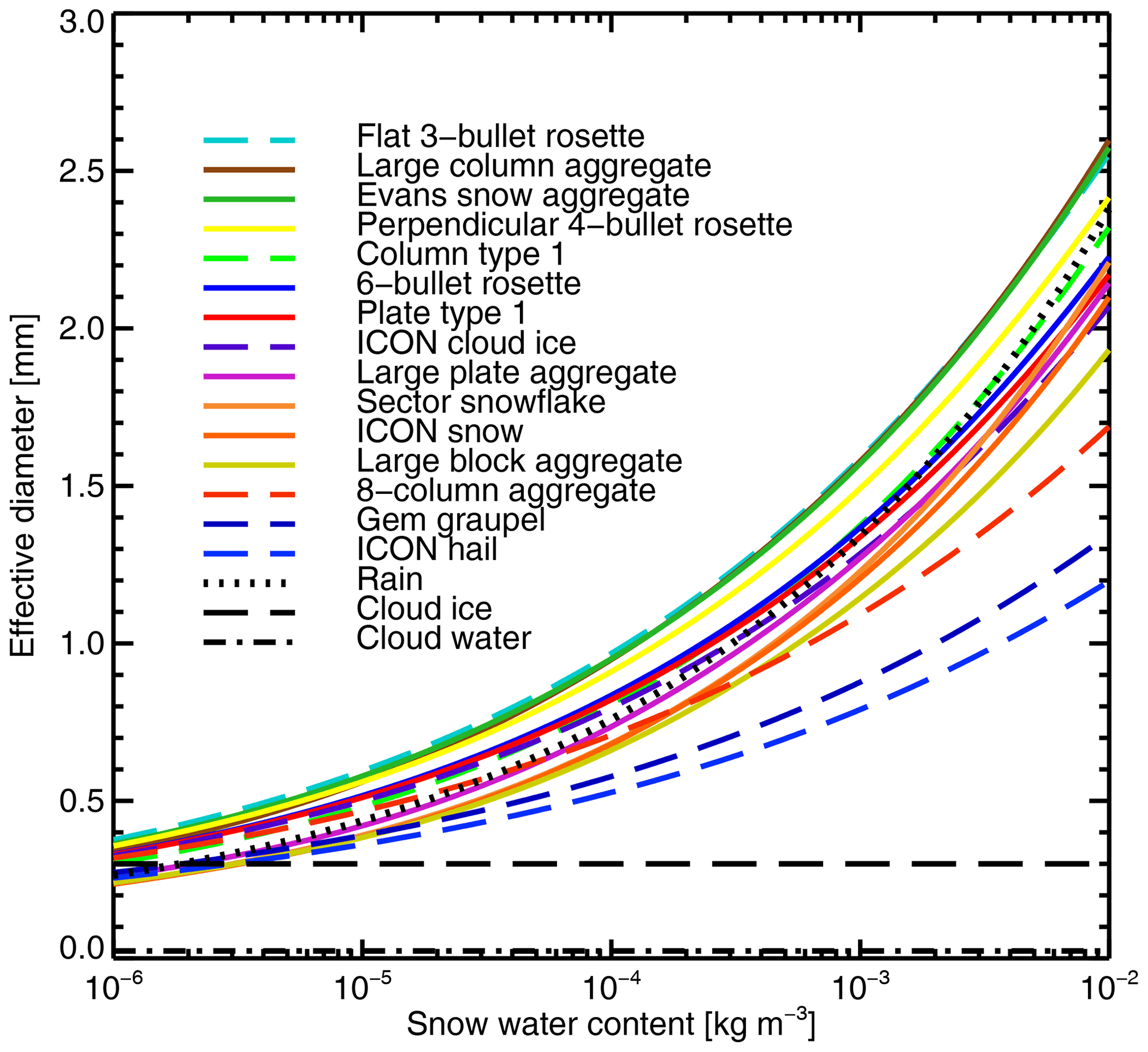
Figure B1 Effective diameter D_eff resulting from the combination of ARTS frozen particles and the F07 T PSD, using all the same settings as Fig. 2. Also shown are the effective diameters of the standard rain, cloud water, and cloud ice configurations from Table 1 and Fig. 1. In the key, the ARTS particles (all coloured lines) are ordered by their effective diameter at the snow water content l= 1 $\times {\mathrm{10}}^{-\mathrm{3}}$ kg m⁻³.

The effective diameter is still important documentation if in future we hope to use the same microphysical assumptions to represent physical processes that do have strong dependence on the geometric cross section: for example, when doing infrared and visible radiative transfer, or if we wish to interface consistently with a model within which the effective diameter is specified. The standard hydrometeor microphysical set-ups for rain, cloud water, and cloud ice (Table 1, Fig. 1) are also shown in the figure and are at least broadly consistent with typical assumptions. The cloud ice and cloud water effective diameter does not vary with water content, which is to be expected from Eqs. (B1) and (9), noting that the relevant MGD-based PSDs (Table 1) hold all parameters constant apart from N₀, which varies with water content.

Appendix C: Two-stream slab cloud with scattering and thermal emission and absorption

The two-stream approximation for radiative transfer is proposed here as a way to compare different sets of bulk optical properties. To simplify the unpolarised full scattering radiative transfer equation, the two-stream approximation assumes the radiance field is constant in each hemisphere (as a function of azimuth and zenith angle) and is hence described by just two variables, the upward and downward radiances I^↑ and I^↓ (Thomas and Stamnes, 1999; Petty, 2006). A second assumption is that backscattering from one hemisphere into another is proportional to the asymmetry parameter g. With these assumptions, the following radiative transfer equations can be defined, which are averaged over all azimuth and zenith angles in each hemisphere:

$$\begin{array}{}\text{(C1)}& {\displaystyle }\begin{array}{rl}& {\displaystyle \frac{\mathrm{1}}{\mathrm{2}}}{\displaystyle \frac{\mathrm{d}{I}^{\uparrow }\left(\mathit{\tau }\right)}{\mathrm{d}\mathit{\tau }}}=\\ & (\mathrm{1}-{\mathit{\omega }}_{\mathrm{0}})\left(I^{\uparrow }\right(\mathit{\tau })-B)+{\displaystyle \frac{{\mathit{\omega }}_{\mathrm{0}}(\mathrm{1}-g)}{\mathrm{2}}}\left(I^{\uparrow }\right(\mathit{\tau })-I^{\downarrow }(\mathit{\tau }\left)\right)\end{array}\text{(C2)}& {\displaystyle }\begin{array}{rl}& -{\displaystyle \frac{\mathrm{1}}{\mathrm{2}}}{\displaystyle \frac{\mathrm{d}{I}^{\downarrow }\left(\mathit{\tau }\right)}{\mathrm{d}\mathit{\tau }}}=\\ & (\mathrm{1}-{\mathit{\omega }}_{\mathrm{0}})\left(I^{\downarrow }\right(\mathit{\tau })-B)-{\displaystyle \frac{{\mathit{\omega }}_{\mathrm{0}}(\mathrm{1}-g)}{\mathrm{2}}}\left(I^{\uparrow }\right(\mathit{\tau })-I^{\downarrow }(\mathit{\tau }\left)\right)\end{array}.\end{array}$$

This follows the derivation in Petty (2006) but does not drop the Planck function B, so it represents thermal emission as well as scattering. The single scattering albedo ω₀, asymmetry g, and temperature (and hence Planck function B) are assumed to be constant in optical depth τ. Adding and subtracting Eqs. (C1) and (C2), then differentiating, and then substituting again from Eqs. (C1) and (C2) gives

$$\begin{array}{}\text{(C3)}& {\displaystyle \frac{{\mathrm{d}}^{\mathrm{2}}}{\mathrm{d}{\mathit{\tau }}^{\mathrm{2}}}}\left(I^{\uparrow }\right(\mathit{\tau })+I^{\downarrow }(\mathit{\tau }\left)\right)={\mathrm{{\rm Y}}}^{\mathrm{2}}\left[\left(I^{\uparrow }\right(\mathit{\tau })+I^{\downarrow }(\mathit{\tau }\left)\right)-\mathrm{2}B\right];\text{(C4)}& {\displaystyle \frac{{\mathrm{d}}^{\mathrm{2}}}{\mathrm{d}{\mathit{\tau }}^{\mathrm{2}}}}\left(I^{\uparrow }\right(\mathit{\tau })-I^{\downarrow }(\mathit{\tau }\left)\right)={\mathrm{{\rm Y}}}^{\mathrm{2}}\left(I^{\uparrow }\right(\mathit{\tau })-I^{\downarrow }(\mathit{\tau }\left)\right),\end{array}$$

where Υ has been defined in Eq. (23). These equations have generally known solutions, so

$$\begin{array}{}\text{(C5)}& {\displaystyle }{I}^{\uparrow }\left(\mathit{\tau }\right)+I^{\downarrow }\left(\mathit{\tau }\right)=c_{\text{1}}\text{exp}\left(\mathrm{{\rm Y}}\mathit{\tau }\right)+c_{\text{2}}\text{exp}(-\mathrm{{\rm Y}}\mathit{\tau })+\mathrm{2}B;\text{(C6)}& {\displaystyle }{I}^{\uparrow }\left(\mathit{\tau }\right)-I^{\downarrow }\left(\mathit{\tau }\right)=c_{\text{3}}\text{exp}\left(\mathrm{{\rm Y}}\mathit{\tau }\right)+c_{\text{4}}\text{exp}(-\mathrm{{\rm Y}}\mathit{\tau }).\end{array}$$

Here, c₁ to c₄ are coefficients that need to be found. Further manipulation, similar to Petty (2006), gives the solutions for the upward and downward radiances:

$$\begin{array}{}\text{(C7)}& {\displaystyle }{I}^{\uparrow }\left(\mathit{\tau }\right)=A\text{exp}\left(\mathrm{{\rm Y}}\mathit{\tau }\right)+r_{\mathrm{\infty }}D\text{exp}(-\mathrm{{\rm Y}}\mathit{\tau })+B;\text{(C8)}& {\displaystyle }{I}^{\downarrow }\left(\mathit{\tau }\right)=r_{\mathrm{\infty }}A\text{exp}\left(\mathrm{{\rm Y}}\mathit{\tau }\right)+D\text{exp}(-\mathrm{{\rm Y}}\mathit{\tau })+B.\end{array}$$

Here, A and D are constants deriving from c₁ to c₄ that still need to be determined. r_∞ is the cloud albedo, a function of ω₀ and asymmetry g defined earlier. The constants are found by imposing the boundary conditions $I^{\downarrow }\left({\mathit{\tau }}^{*}\right)=\mathrm{0}$ and $I^{\uparrow }\left({\mathit{\tau }}^{*}\right)=I_{\mathrm{0}}$, in other words zero downward radiation at the top of the cloud, and a fixed amount of radiation upwelling from below the cloud. The boundaries are hence assumed to be black bodies, unaffected by the radiation emitted from the cloud. This gives

$$\begin{array}{}\text{(C9)}& {\displaystyle }{I}_{\mathrm{0}}=A\exp \left(\mathrm{{\rm Y}}{\mathit{\tau }}^{*}\right)+r_{\mathrm{\infty }}D\exp (-\mathrm{{\rm Y}}{\mathit{\tau }}^{*})+B;\text{(C10)}& {\displaystyle }\mathrm{0}=r_{\mathrm{\infty }}A+D+B.\end{array}$$

These can be easily solved for A and D, and the radiation emitted at the top of the cloud I^↑(0) can be determined from Eq. (C7) to provide Eq. (21). Setting B=0 recovers the two-stream pure-scattering example from Petty (2006, his Eqs. 13.39 and 13.40). Setting I₀=0 and g=0 (no external radiation sources, isotropic scattering) recovers the “imbedded source” solution from Thomas and Stamnes (1999, their Eqs. 7.69 and 7.70).