the Creative Commons Attribution 4.0 License.
the Creative Commons Attribution 4.0 License.
 | 07 Dec 2021
MagIC v5.10: a two-dimensional message-passing interface (MPI) distribution for pseudo-spectral magnetohydrodynamics simulations in spherical geometry
Rafael Lago
Thomas Gastine
Tilman Dannert
Markus Rampp
Johannes Wicht
We discuss two parallelization schemes for MagIC, an open-source, high-performance, pseudo-spectral code for the numerical solution of the magnetohydrodynamics equations in a rotating spherical shell. MagIC calculates the non-linear terms on a numerical grid in spherical coordinates, while the time step updates are performed on radial grid points with a spherical harmonic representation of the lateral directions. Several transforms are required to switch between the different representations. The established hybrid parallelization of MagIC uses message-passing interface (MPI) distribution in radius and relies on existing fast spherical transforms using OpenMP. Our new two-dimensional MPI decomposition implementation also distributes the latitudes or the azimuthal wavenumbers across the available MPI tasks and compute cores. We discuss several non-trivial algorithmic optimizations and the different data distribution layouts employed by our scheme. In particular, the two-dimensional distribution data layout yields a code that strongly scales well beyond the limit of the current one-dimensional distribution. We also show that the two-dimensional distribution implementation, although not yet fully optimized, can already be faster than the existing finely optimized hybrid parallelization when using many thousands of CPU cores. Our analysis indicates that the two-dimensional distribution variant can be further optimized to also surpass the performance of the one-dimensional distribution for a few thousand cores.
- Article
(3944 KB) - Full-text XML
- BibTeX
- EndNote


The dynamics in many astrophysical objects like stars, planets, or moons are aptly modelled by the fluid flow and magnetic field generation in a rotating sphere or spherical shell. Since the pioneering work by Glatzmaier (1984), several numerical codes have been developed over the years to model the problem. Typically, they all solve for convection and magnetic field induction in a co-rotating reference frame. The solutions are formulated as disturbances about a hydrostatic, well-mixed, and adiabatic reference state. The so-called Boussinesq approximation assumes a homogeneous background state and yields a particularly simple formulation. Meanwhile, the anelastic approximation (e.g. Lantz and Fan, 1999; Jones et al., 2011) allows the incorporation of radial variation of the background reference state and transport properties. While the Boussinesq approximation seems appropriate for modelling the liquid cores of terrestrial planets, the anelastic approximation is more relevant for gas planets or stars for which the density contrasts are very large.
MagIC (2021), the open-source code extensively discussed here, allows for the choice of either Boussinesq or anelastic approximation. The initial implementation by Glatzmaier (1984), originally geared towards modelling the solar convective zone, split into two separate codes in the 1990s. One code version was used to model the first numerical geodynamo (Glatzmaier and Roberts, 1995) and was later adopted and modified by Olson et al. (1999) to a Boussinesq code named MAG (2021). This modified code formed the basis for an earlier version of MagIC (Wicht, 2002). Stellar dynamo models were carried out using a more efficient version of the original Glatzmaier (1984) code named ASH (anelastic spherical harmonic; see Clune et al., 1999), which more recently led to the open-source code Rayleigh (2021) (Featherstone, 2018).
MagIC still mostly follows the original algorithm laid down by Glatzmaier (1984). It is a pseudo-spectral code written in modern Fortran. Pseudo-spectral algorithms use a spectral representation to compute accurate derivatives and a grid representation for calculating non-linear terms. In MagIC, the angular representation switches between a longitude–latitude grid and a spherical harmonic representation. Chebyshev polynomials are used for the spectral representation in radius, but MagIC also offers to employ finite differences instead. Different implicit–explicit time-stepping schemes (IMEX) are available, wherein the non-linear terms and the Coriolis force are treated explicitly, while the stiff linear terms are handled implicitly.
Over the last 20 years several aspects of the original algorithm by Glatzmaier (1984) have been tested against alternative ideas. Among them are radial discretization algorithms based on finite differences (Dormy et al., 1998), compact finite differences (Takahashi, 2012), and a sparse Chebyshev formulation (Marti et al., 2016). Various different implicit–explicit strategies for the time stepping have also been studied (e.g. Livermore, 2007; Garcia et al., 2010; Marti et al., 2016).
For the last 20 years, MagIC simulations have resulted in more than 120 peer-reviewed publications (See https://ui.adsabs.harvard.edu/user/libraries/LVt1vdaKQsC5P09In2iloA, last access: 20 October 2020). They cover a broad range of scientific fields, including fundamental fluid dynamics in spherical geometry (e.g. Wicht, 2014; Barik et al., 2018), numerical modelling of the geodynamo (e.g. Wicht, 2002), and modelling of planetary (e.g. Gastine and Wicht, 2012; Heimpel et al., 2016) and stellar (e.g. Gastine et al., 2014; Raynaud et al., 2020) internal dynamics. The code has been tested and validated by community-driven comparison benchmarks for Boussinesq convection (Christensen et al., 2001), anelastic convection (Jones et al., 2011), double-diffusive convection (Breuer et al., 2010), and convection in full spheres (Marti et al., 2014). Several publications concern the study of the solid Earth and its magnetic field. For instance, MagIC was used to study the “top-heavy” regime of double-diffusive convection when thermal and compositional background gradients are destabilizing (Tassin et al., 2021). In a recent paper, MagIC has been used to study magnetic boundary layers with heterogeneous outer boundary heat flux, with results suggesting a significant deviation from classical estimates of the diffusion time and the magnetic Reynolds number (Terra-Nova and Amit, 2020). In another paper, the dynamics of a possible stable stratification layer atop Earth's core were explored (e.g. Gastine et al., 2020), leading to the conclusion that such a layer would lead to strong magnetic skin effects incompatible with current observations.
Achieving an efficient use of the available computer resources by a given numerical implementation often proves challenging, in particular when moving to petascale architectures. There are two main reasons. First, the large number of physical compute cores requires a large enough workload that can be fairly partitioned and distributed across these processing units. This typically puts an upper bound on the number of cores that can usefully be employed and often results in poor strong scaling. A second complication arises from the different layers of memory access and of communication between the physical cores (i.e. non-uniform memory access – NUMA – domains, sockets, nodes). Ideally, one would attempt to keep all data “local” for quick access. However, optimizing a code for properly distributing the workload while keeping a reasonable data locality can be difficult and often requires compromising one aspect in favour of another.
Until recently, MagIC only offered a one-dimensional distribution of the data implemented using MPI+OpenMP (hereafter referred to as “1d-hybrid” implementation). For calculating the non-linear terms in grid space, this code uses MPI to distribute the spherical shells between the available NUMA domains and the inherent OpenMP scheme of the open-source spherical harmonics transform library SHTns (2021) (Schaeffer, 2013) for computations within a NUMA domain. Since MagIC is not optimized for multithreading between NUMA domains, this configures a limitation on the maximum number of the radial grid points. This limitation could be quite severe. High-performance computing (HPC) clusters typically offer two NUMA domains per compute node, but the current trend in hardware development might lead into a further subdivision into multiple physical units (e.g. AMD EPYC and Intel CascadeLake-AP) or logical NUMA domains (e.g. sub-NUMA clustering in Intel Xeon). Effectively, the computing power per NUMA domain has stagnated and it may even decrease in the future. This would simply prevent MagIC from taking advantage of performance gains in the foreseeable evolution of processor technology. In addition, numerical experiments in Matsui et al. (2016) suggest that two- or three-dimensional parallelization might be necessary for dynamo codes to achieve petascale capabilities with current hardware architecture.
The first two-dimensional MPI domain decomposition in pseudo-spectral codes in spherical geometry was considered in the ASH code by Clune et al. (1999). The layout was nevertheless still not completely two-dimensional in the sense that the maximum number of MPI ranks was still bounded by the maximum spherical harmonic degree. This limitation was released in more recent implementations by Marti and Jackson (2016) in the context of modelling full spheres, by Matsui et al. (2014) in the geodynamo code Calypso (2021), and in the Rayleigh code. The performance benchmark by Matsui et al. (2016), however, revealed an important overhead for these codes compared to pseudo-spectral codes which avoid global communications such as the open-source code XSHELLS (2021) (e.g. Schaeffer et al., 2017).
Motivated by the aforementioned points, we propose in this work a two-dimensional data distribution layout for MagIC with communication-avoiding features. This required a major rethinking of data structures and communication algorithms, and it demands a re-implementation and thorough optimization of a large portion of the existing 1d-hybrid code. Due to the high complexity of the required refactoring tasks, OpenMP parallelism was dropped from the current implementation for the time being. Since the two-dimensional distribution implementation presented here relies on pure MPI communication, we refer to it as the “2d-MPI” implementation or version. Implications and incentives to eventually re-introduce OpenMP into the new version will be discussed along the way.
This paper is organized as follows. In Sect. 2 we provide an overview of the mathematical formulation and the numerical techniques used in MagIC. In Sect. 3 we detail the pseudocodes for the sequential algorithm for the 1d-hybrid and the 2d-MPI implementations. We also describe the underlying data structures and the key differences between each approach. In Sect. 4 we thoroughly compare the different parts of 1d-hybrid and 2d-MPI implementations. We focus our discussion on the strong scaling of both algorithms, but we also discuss the raw performance in different regimes. In Sect. 4.5 we show the performance and parallel efficiency of both implementations. In Sect. 4.6 we focus on analysing the main bottleneck of the 2d-MPI implementation and discuss the viability of further performance improvements and their expected impact. Finally, in Sect. 5 we summarize our findings.
In this section we introduce aspects of the numerical formulation which are relevant for the understanding of this work. Since the implementation of the magnetohydrodynamic (or MHD for short) equations implemented in MagIC still closely follows the original work by Glatzmaier (1984), we refer to this publication and to more recent reviews (e.g. Tilgner, 1999; Hollerbach, 2000; Christensen and Wicht, 2015) for a more comprehensive description of the algorithm.
2.1 Dynamo model
We consider a spherical shell of inner radius ri and outer radius ro rotating about the z axis with a constant frequency Ω. Convective motions are driven by a fixed temperature contrast ΔT between the two boundaries. We adopt a dimensionless formulation of the MHD equations using the shell gap as the reference length scale and the viscous diffusion time as a time unit. Velocity is dimensionlessly represented in units , temperature in units ΔT, and the magnetic field in units , where μ is the magnetic permeability, ν the kinematic viscosity, and λ the magnetic diffusivity. The dimensionless equations that control the time evolution of the velocity u, the magnetic field B, and the temperature T under the Boussinesq approximation read
where p is the non-hydrostatic pressure, er and ez are the unit vectors along the radial and axial directions, respectively, and is the dimensionless self-gravity. This set of equations is controlled by four dimensionless parameters, the Rayleigh number Ra, the Ekman number E, the magnetic Prandtl number Pm, and the Prandtl number Pr:
where α is the thermal expansivity, go is the gravity at the outer boundary, and κ is the thermal diffusivity. Equations (1)–(4) need to be complemented by appropriate boundary conditions for temperature, velocity, and magnetic field as well as an initial state.
2.2 Spatial discretization
To ensure the solenoidal nature of u and B, Eqs. (2)–(4) are solved in the spherical coordinates by expanding the velocity and the magnetic fields into poloidal and toroidal potentials following
This formulation yields the six time-dependent scalar quantities W, Z, G, H, T, and p. These six variables are expanded in spherical harmonic functions up to a degree and order ℓmax in the angular directions (θ,ϕ). Since the spherical harmonics are the set of eigenfunctions of the Laplace operator on the unit sphere, they are an especially attractive basis for representing functions in spherical coordinates. They are defined by
where Pℓm represents the normalized associated Legendre polynomials (see Abramowitz and Stegun, 1964). Any function at the radius r and instant t can be expanded by a truncated spherical harmonic decomposition:
Letting ⋆ denote the complex conjugate, it holds that for all real functions f. This effectively halves the cost of computing and storing the spherical harmonic coefficients.
Reordering the terms in Eq. (7) and using the definition of the spherical harmonics from Eq. (6) we obtain
which is known as the inverse spherical harmonics transform. By integrating fℓmYℓm over the spherical coordinates using the Gauss–Legendre quadrature we obtain the forward transform:
where θj and wj are respectively the Gauss nodes and weights for the Nθ collocation points in the latitudinal direction, and represents the Nϕ regularly spaced grid points in the azimuthal direction.
The formulation discussed in Eqs. (8)–(11) provides a two-step algorithm for computing the spherical harmonics transforms (hereafter SHTs) corresponding to a Legendre transform and a Fourier transform. The latter can be handled by finely optimized implementations of the fast Fourier transform (FFT for short) such as the FFTW library (Frigo and Johnson, 2005), which costs 𝒪(Nϕlog Nϕ) operations. There is no fast transform for Eq. (11), and the complexity of an individual Legendre transform scales as operations. In MagIC, we use the open-source library SHTns (2021) for SHTs and Legendre transforms (Schaeffer, 2013), which relies on the recurrence relation by Ishioka (2018). Additionally, in the context of practical numerical implementation, a transposition is required between the two transforms; this will be covered further in Sect. 3.
The quadrature shown in Eq. (11) is exact for Nθ>ℓmax (Schaeffer, 2013), but in practice, we set in order to prevent aliasing errors (e.g. Orszag, 1971; Boyd, 2001). In fact, we also set Nϕ=2Nθ for the number of longitudinal points, which guarantees isotropic resolution in the equatorial regions (Glatzmaier, 2013).
During the initialization stage, MagIC allows the choice between finite differences or a spectral expansion using Chebyshev polynomials to handle the radial discretization strategy. Finite-difference methods allow the use of faster point-to-point communications, but they also require a larger number of nodal points to ensure a proper convergence of the solution. In this work, we explicitly chose to focus solely on the spectral approach to handle the radial discretization, but we encourage the interested reader to consult Matsui et al. (2016) for an extensive comparison between several different numerical implementations.
Each spectral coefficient fℓm(r,t) is expanded in truncated Chebyshev series up to the degree Nc−1:
where is a normalization factor and the double quotes mean that the first and last terms need to be multiplied by one-half. In the above expression, Cn(x) is the nth-order first-kind Chebyshev polynomial defined by
with
the kth nodal point of a Gauss–Lobatto grid defined with Nr collocation points. The discrete radius rk defined between ri and ro is mapped onto xk using the following affine mapping:
Conversely, the Chebyshev spectral coefficients of the functions fℓm(r,t) read
With the particular choice of Gauss–Lobatto collocation points, Eqs. (12) and (13) can also be efficiently computed using fast discrete cosine transforms (DCTs) of the first kind (Press et al., 2007, Sect. 12.4.2).
2.3 Time discretization
With the spatial discretization fully specified, we can proceed with the time discretization. For an easier understanding, we will derive the main steps using the equation for the time evolution of the magnetic poloidal potential G as an illustrative example. We refer the interested reader to e.g. Christensen and Wicht (2015) or the online documentation of MagIC for the derivation of the other equations.
The equation for G is obtained by considering the radial component of the induction equation (see Eq. 3). Using the spherical harmonics decomposition and the Chebyshev collocation method described above we obtain
where is the second radial derivative of the nth Chebyshev polynomial and d𝒮=sin θ dθdϕ is the spherical surface element.
Equation (14) can be rewritten in the following matrix form:
where the matrices Aℓ and contain primarily the coefficients of Cn(xk) and , are dense, and depend on ℓ but not on m. Equation (15) forms a set of ordinary differential equations that depend on time and contain a non-linear term, namely , and a stiff linear diffusion operator.
In order to mitigate the time step constraints associated with an explicit treatment of the diffusion terms, MagIC adopts an implicit–explicit (IMEX) time-stepping approach. Non-linear and Coriolis terms are handled using the explicit part of the time integrator, while the remaining linear terms are treated implicitly. Currently, IMEX multisteps (e.g. Ascher et al., 1995) or IMEX diagonally implicit Runge–Kutta (DIRK; e.g. Ascher et al., 1997) are available.
Let δt denote the time step size. A general k step IMEX multistep method applied to Eq. (15) reads
where the exponent notations correspond to the time discretization with and aj, , and corresponds to the weights of the IMEX multistep scheme. In practice, multistep schemes present stability domains that decrease with their order of convergence and require knowledge of past states to continue the time integration. As such, they are not self-starting and need to be initiated with a lower order scheme. MagIC implements DIRK schemes to overcome these limitations, but here we discuss only a simple two-step IMEX scheme. Setting the IMEX weights to , and , Eq. (16) reduces to the popular IMEX scheme assembled from a Crank–Nicolson and a second-order Adams–Bashforth scheme (Glatzmaier, 1984) and can simply be written as
with and respectively defined by the underbraces on the left- and right-hand side of Eq. (17). Assuming suitable initial and boundaries conditions, all terms needed to compute are known from the previous iterations. The matrices contain the Chebyshev coefficients and are dense but real-valued and of moderate size (realistic values of Nr range from 33 to 1025). As such, the linear system in Eq. (17) typically requires operations to be inverted (Boyd, 2001) and can be easily solved using LU decomposition and backward substitution from standard libraries such as LAPACK (Anderson et al., 1999). From here on, we generalize the notation and use Eq. (17) when discussing the time stepping for any fields, i.e. not only the magnetic poloidal potential G.
MagIC is a highly optimized hybrid MPI+OpenMP code under active development. The 1d-hybrid version uses MPI to distribute the Nr spherical shells amongst different computing nodes, while employing OpenMP for fully using the local cores within an individual NUMA domain. Although MagIC is finely optimized, multithreading across NUMA domains is not implemented. Therefore, simulations require at least one spherical shell per NUMA domain. This restricts the maximum number of NUMA domains to Nr−1, which severely limits the computational resources that can be employed for a given radial resolution. This disadvantage could increase in the future since the current trend in HPC architecture is to further subdivide the computing units into physical or even logical NUMA domains.
The purpose of this section is to first familiarize the reader with the established 1d-hybrid implementation and then introduce the new 2d-MPI implementation. By adding MPI parallelism in a second direction, the extension also allows distributing the computations within a shell over the NUMA domains, sockets, or even nodes of a computer cluster.
Due to the high complexity of this re-implementation, our 2d-MPI version lacks any use of OpenMP. The main purpose of this work is to provide a thorough assessment of the prospects and merits of a two-dimensional data distribution, to pinpoint shortcomings, and to discuss the overall viability of a possible fully optimized and fine-tuned two-dimensional distribution implemented using OpenMP+MPI.
In this section we first present the pseudocode for the sequential algorithm for MagIC in Sect. 3.1 and then discuss the distribution of the data for both the 1d-hybrid and 2d-MPI versions in Sect. 3.2. A more detailed description of the two main parts of the code is discussed in Sect. 3.3 and 3.4.
3.1 Sequential algorithm
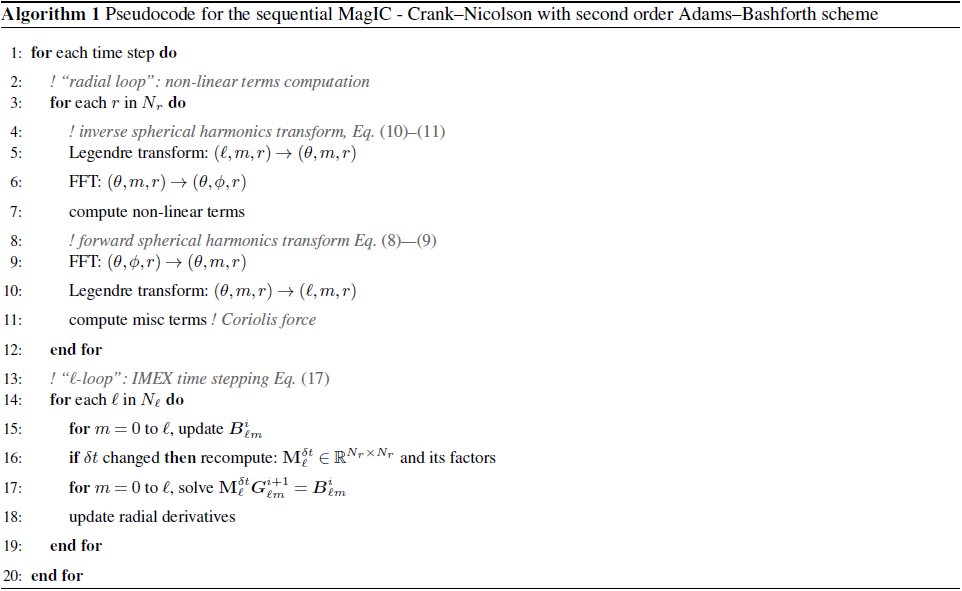
For the sake of simplicity, we discuss only the second order time-stepping scheme described in Sect. 2.3, Eq. (17). The resulting pseudocode is shown in Algorithm 1. For each time step, the code can be divided into two stages, the “radial loop” and the “ℓ loop”.
The radial loop (lines 2–10). It computes the non-linear terms in grid space and thus requires forward and inverse SHTs. The radial levels are completely decoupled in this stage and can thus be efficiently distributed without any need for communication between them. The directions (ℓ,m) and (θ,ϕ) are coupled. Notice that the FFTs on lines 6 and 9 take place on the second, slowest dimension. This requires the Fourier transform to “stride” the data in memory. This is not ideal, but modern FFT libraries are able to efficiently handle strided transforms.
The ℓ loop (lines 13–18). It performs the actual time step. Most of the computational effort goes into solving
the linear systems from Eq. (17) and into updating the right-hand-side .
After updating each , the factors of are computed using LAPACK's
real-valued LU decomposition dgetrf routines for dense matrices. Next, the solution of each linear system from
Eq. (17) needs to be computed. In practice,
all right-hand sides are “packed” in a real matrix :
where ℜ and ℑ respectively represent the real and imaginary parts of the vector. The system is then solved for all right-hand sides as
with a single call to LAPACK's dgetrs. The matrix is computed and stored as
for faster memory access during the LAPACK call. Therefore, the intermediate solution X is also obtained as
. The final solution is reconstructed from X by reordering the data back into
the format, while adding the real and imaginary parts back together.
Also notice that the decomposed factors of are kept for all subsequent time steps and are only
recomputed when δt changes.
3.2 Data distribution
In this section we discuss how the simulation is distributed across MPI ranks for the 1d-hybrid and the 2d-MPI implementations. For all purposes, MPI Cartesian grid topology is used. The ϕ direction is numerically periodic, but this property is never explicitly used by the underlying algorithms. The remaining directions are non-periodic. We denote by Πr the number of MPI ranks used in the radial direction. Similarly, Πθ represents the number of ranks in the θ or ℓ direction.
Let denote the total number of ℓ modes, Nm the number of m modes, and Nℓm the number of (ℓ,m) tuples. We simply use the − superscript to denote the number of local points in some MPI rank. For instance, denotes the number of local radial points stored in a given rank.
1d-hybrid distribution. In the radial loop, the data distribution for the 1d-hybrid approach follows intuitively from Algorithm 1. The radial shells are distributed evenly among the MPI ranks, ideally for each rank. During the computation of the non-linear terms, each rank stores points. During the computation of the miscellaneous terms, each rank stores points.
This changes for the execution of the ℓ loop. For efficiently computing line 17 of Algorithm 1, all Nr radial points must be local. This is achieved by the so-called ℓ transposition, which changes the data distribution to local points. Special care is needed when choosing the distribution of the points. The computational effort per ℓ mode is given by the LU decomposition of the matrix and the solve step for ℓ+1 right-hand-side vectors for this matrix. To balance the computation among the Πr processes, we distribute the ℓ modes in a “snake-like” fashion. Starting with the largest ℓ, which has the highest computational effort, we distribute the ℓ modes over the processors until Πr is reached. The next ℓ is also placed on this last processor, and then we reverse the order until reaching the first processor again. The procedure is repeated until all modes have been distributed. See Fig. 1 for an illustration with Nℓ=21 and Πr=6. This snake-like distribution guarantees that the largest possible imbalance between two MPI ranks is Πr−1 tuples. Furthermore, each matrix can be fully stored locally, which is not the case for the 2d-MPI code, as we discuss below. At the end of the ℓ loop, another ℓ transposition takes place, converting the data layout back to local points.
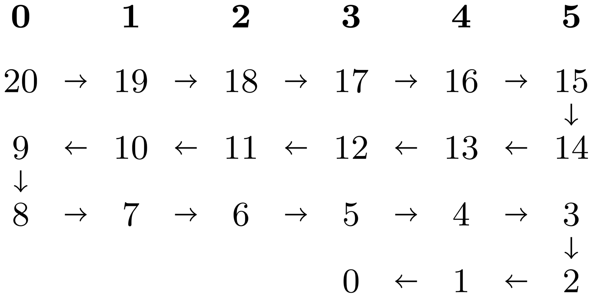
Figure 1Illustration of the “snake ordering” of the (ℓ,m) tuples for the 1d-hybrid distribution with Nℓ=21 and Πr=6. The top row shows the processor number in boldface, and the remaining numbers indicate the ℓ modes; ℓ+1 solution steps are associated with each ℓ value. The arrows illustrate the snake-like winding pattern of this ordering.
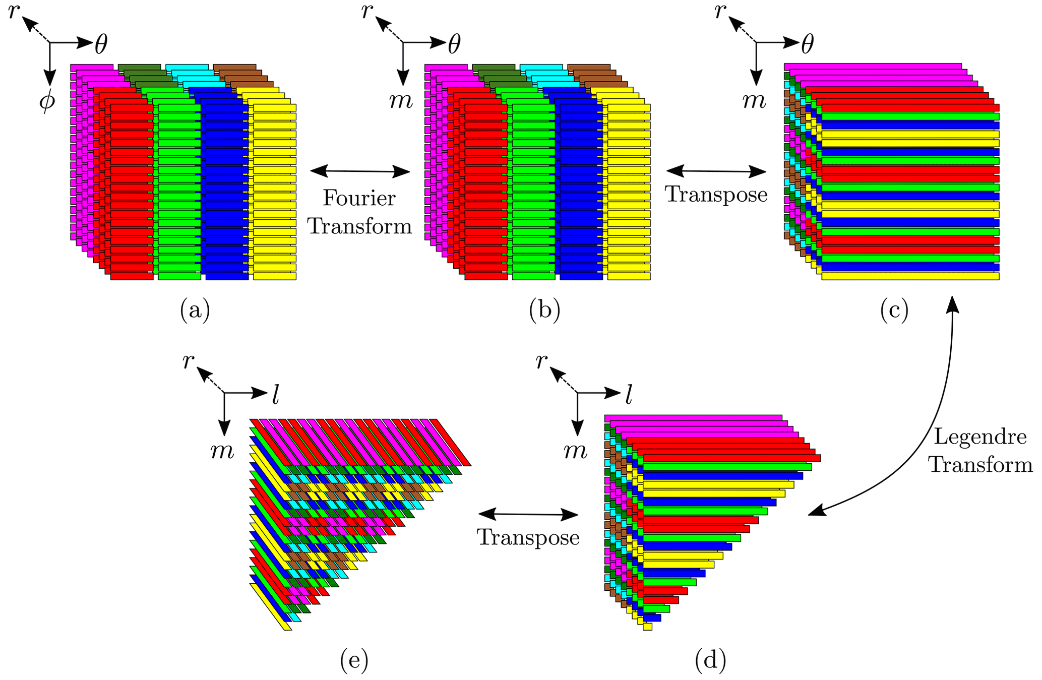
Figure 2Illustration of the 2d-MPI distribution of the points with Πr=2, Πθ=4, Nr=8, and (a more realistic proportion would have been ). Continuous stripes represent continuous memory segments, and different colours represent distinct MPI ranks. The images show which MPI rank would store and process each data segment during (a) computation of non-linear terms, (b–d) forward SHT, and (e) the beginning of the ℓ loop.
2d-MPI distribution. Like in the 1d-hybrid implementation, the radial points are split evenly between the Πr ranks in the radial loop. Additionally, the Nθ points are distributed evenly and contiguously between the Πθ ranks (see Fig. 2a). At line 7, each rank is responsible for the computation of points. After the FFT at line 9 of Algorithm 1, points are stored locally, but the computation of the Legendre transform at line 10 requires all θ angles for a given spherical harmonic order m to be available locally. This is guaranteed by the so-called θ transposition, which gathers the values for all Nθ θ angles while distributing the m modes, resulting in local points.
The distribution of the m modes is more involved than the distribution of the θ angles because there are (Nℓ−m) different spherical harmonic degrees ℓ for each order m. Once again, we employ the snake-like distribution depicted in Fig. 1, which guarantees that the largest imbalance between any two MPI ranks is Πθ−1 tuples. See Fig. 2c–d for a graphical representation of this step.
Just like in the 1d-hybrid implementation, an ℓ transposition is required before the ℓ loop in order to locally gather all Nr radial points. This once again involves a complex redistribution of data points. Because of Eq. (17), we would like to distribute only the ℓ modes while keeping all radial points and m modes local. This would incur an unfeasible volume of data transfer.
We opted for a compromise that exploits a special regularity of the current data structure and leaves the m modes local. Only the Πθ ranks having a common m mode then need to communicate in the radial direction. Figure 2d–e visualize how the respective communication works. Only the magenta and red ranks need to share their radial information since they represent the same m modes. They then also have the same number of ℓ modes and can thus split the number of modes. The snake-like distribution leads to a good balancing for both ranks. The resulting distribution is visualized in Fig. 2e.
The figure also illustrates a drawback of this distribution: the m modes for one l mode can be found on different ranks. This means that the matrices have their columns distributed between MPI ranks and that the time-stepping matrices and their respective decomposition need to be duplicated in Πθ ranks. However, our numerical experiments show that the communication cost far outweighs the cost associated with solving Eq. (17), thus justifying our choice. This will be further discussed in Sect. 4. Finally, we would like to mention that a similar data layout was employed by Marti and Jackson (2016) in their two-dimensional MPI decomposition of their pseudo-spectral code in spherical geometry.
3.3 Radial loop implementation
The spherical harmonics transform (SHT) takes a substantial portion of the runtime. MagIC relies heavily on SHTns (Schaeffer, 2013), a highly optimized library dedicated to computing the spherical harmonics transform using OpenMP, advanced SIMD vectorization, and cache-hitting strategies (Ishioka, 2018). SHTns has been developed to compute the steps synthesized in lines 8–10 and lines 4–6: that is, independent of the radial level r. It can handle scalar fields and is also optimized for general vector fields and vector fields with a poloidal–toroidal decomposition. SHTns is written in C but has a Fortran interface with a dedicated data layout for MagIC. Although SHTns is flexible and modular, it does not have an MPI-distributed interface. However, it offers an interface for computing the Legendre transform (lines 5 and 10 of Algorithm 1) only for an individual (m,r) pair, which is the use case in our 2d-MPI implementation. The transposition and FFT computations are then handled separately by MagIC.
Next we describe how both the 1d-hybrid and 2d-MPI version of the code use SHTns for computing the SHT.
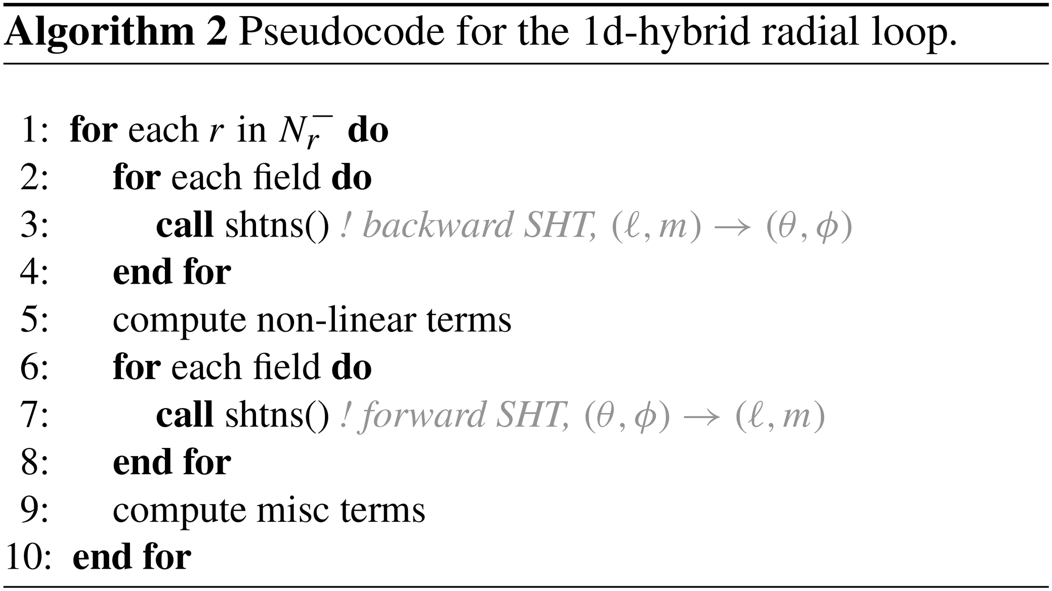
1d-hybrid radial loop.
The spherical harmonics transforms are delegated directly to SHTns (see the pseudocode in Algorithm 2).
For instance, for the temperature scalar field on the numerical grid, , a single
call to spat_to_SH returns the fully transformed Tℓm(rk) for a given radial level rk. This is only possible because
all (θ,ϕ) points are local in the 1d-hybrid version of the code. No explicit optimization or multithreading is
required, as SHTns handles this internally. The number of vector transforms needed per radial loop depends on the set of equations.
Dynamo models under the Boussinesq approximation of the Navier–Stokes equations considered here (Eqs. 1–4)
involve four vector transforms and one scalar transform for the backward SHTs and three vector transforms for the forward SHTs.
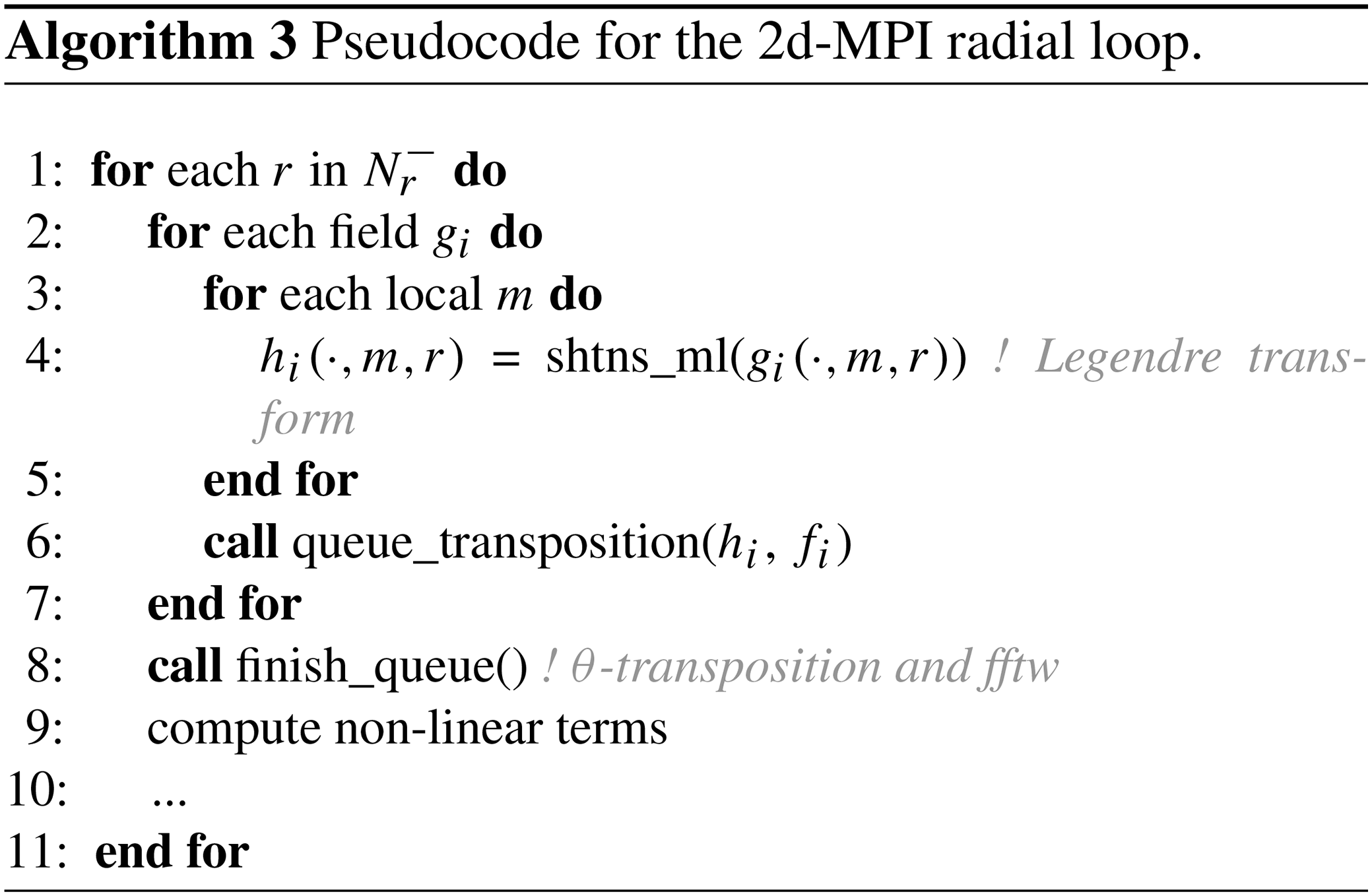
2d-MPI radial loop.
The pseudocode for our implementation is shown in Algorithm 3. Since shtns_ml is called for single modes only, the
implementation cannot benefit from the efficient internal OpenMP parallelization of SHTns. The computation time for only a single mode is
too small to justify the initialization and termination of a multithreading context. In addition, the larger number
of SHTns calls causes some overhead.
Some speed-up could possibly be gained with an OpenMP parallelization of the SHTns calls (lines 3–5 in
Algorithm 3) or directly at the radial loop level (line 1 in Algorithm 3).
Some preliminary tests showed promising results for the former. However, here we shall continue discussing only the pure MPI version.
The so-called θ transposition happens in line 8 of Algorithm 3 and involves MPI communication.
Pointers to the input fields hi and output fields fi are ordered in a queue. Upon calling finish_queue, each hi
is effectively transposed. After receiving the data, a complex-to-real FFT (e.g. using Intel MKL, 2021) is performed and saved into the output fields fi.
The queue has a limited size. Once the limit is reached, finish_queue is called, immediately triggering the data
transfer and the FFT computation. Additionally, upon exiting the loop, finish_queue is called one last time to treat
any remaining field in the queue.
The θ transposition is implemented using the following algorithms.
-
P2P: each θ rank performs one call to
mpi_isendandmpi_irecvfor each other θ rank (i.e. Πθ−1) for all queued fields, followed by anmpi_waitallcall. MPI types are used to stride the data when needed. The advantage of this algorithm is that it does not require any particular packing and/or reordering of the data. -
A2AW: a single call to
mpi_alltoallwis performed for all queued fields using the same MPI types used for the P2P algorithm. -
A2AV: a single call to
mpi_alltoallvis performed for all queued fields. No MPI types are needed, but the data need to be reordered in a buffer prior to the call.
Two parameters need to be determined, namely which MPI algorithm to use and the length of the queue. The choice of the MPI algorithm depends on the MPI implementation, the hardware, and the number of resources. We compare the performance of each variant in Sect. 4.1.
As for the length of the θ-transposition queue, several factors must be taken into account.
Longer queues allow more scalar fields to be packed per call, thus allowing larger message size and
decreasing the impact of the latencies of the MPI calls. On the other hand, longer queues require larger
send and receive buffers. The benefit of having larger message sizes may be not relevant for all configurations,
especially if all θ ranks are located within the same NUMA domain (for instance, the Intel implementation of mpi_alltoallv automatically
uses shared-memory operations in this regime). Furthermore, larger queue sizes do not guarantee full usage of the buffers.
We discuss this in more detail in Sect. 4.1.
3.4 The ℓ-loop implementation
As discussed in Sect. 3.2, the data need to be redistributed with the so-called ℓ transposition prior to the execution of this part of the code. The distribution of the ℓ modes and their respective m modes to the MPI processes has already been discussed in Sect. 3.2.
Most of the wall time of the ℓ loop is spent in the ℓ transposition and in the backward substitution for solving the linear systems from Eq. (17). Depending on how often δt changes, the cost for computing the LU decomposition for each dense matrix might become a bottleneck, but in the scenario investigated during our benchmarks, this was not the case. Nevertheless, a frequent change in δt indicates that the algorithm should be run with a generally smaller time step.
Next we describe the ℓ-loop implementations of both MagIC versions.
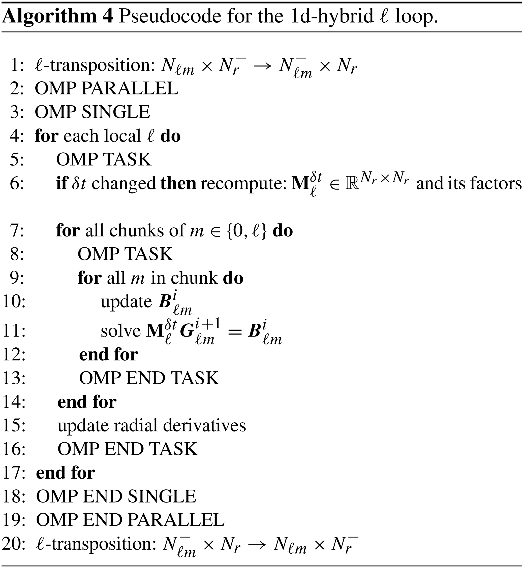
1d-hybrid ℓ loop. The pseudocode is shown in Algorithm 4. The ℓ transposition itself takes place in lines 1 and 20 of Algorithm 4. Inside one MPI rank, the work is parallelized with OpenMP. We have a two-level loop structure, with an outer loop over the different ℓ degrees on the MPI rank and for each ℓ a loop over all possible m≤ℓ. A single OpenMP parallelization of the outer loop would directly compete with the MPI parallelization and would also lead to a strong load imbalance as the different harmonic degrees have different numbers of m. To avoid nested OpenMP regions (for the outer and inner loop) we use the OpenMP tasking approach instead to balance the work and to combine the parallelism of the outer and inner loop. We create an OpenMP task for each outer loop iteration which contains the LU decomposition of the matrix and a task creation loop for the inner m loop. To minimize the overhead for OpenMP task creation, we use chunks of several m together in one task.
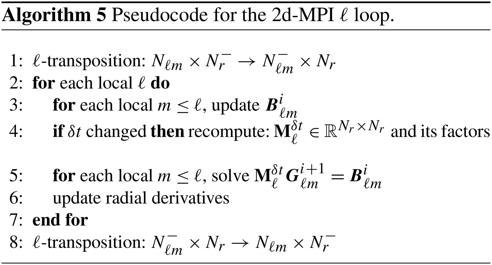
2d-MPI ℓ loop. The pseudocode for the ℓ loop in the sequential and the 2d-MPI implementations (see Algorithm 5) differs only in the ℓ transpositions and the number of ℓ and m modes stored locally (which consequently affects the number of linear systems and right-hand sides in each rank). The distribution of the (ℓ,m) tuples has already been discussed in Sect. 3.2. While the difference in the number of modes has an impact on the computation of the solution of Eq. (17), this pales in comparison with the time spent in communication.
In both the 1d-hybrid and 2d-MPI implementations the ℓ transposition might be performed using the P2P, A2AV, and A2AW algorithms discussed previously. Additionally, the following algorithm has been implemented.
-
A2AP: a single call to
mpi_alltoallper scalar field is performed with padding to accommodate the largest message. No MPI types are needed, but the data need to be reordered in a buffer. Due to the intrinsic imbalance in the distribution of the data, considerably larger buffers are required. Some MPI libraries implement faster algorithms formpi_alltoall, which can in some cases be advantageous.
In the 1d-hybrid implementation of MagIC an auto-tuning routine always selects the optimal transposition strategy during the initialization stage of the code. For the 2d-MPI version, the algorithm still must be selected manually via the parameter file. We discuss the performance of the different strategies in Sect. 4.4.
In this section we compare the performance of the 1d-hybrid and 2d-MPI implementations in a practical, realistic setting. We also profile some crucial sections of the code in order to highlight the advantages and shortcomings of the different implementations.
Following Matsui et al. (2016), we adopt the dynamo benchmark “BM1” from Christensen et al. (2001) to assess the performance of the code. The benchmark uses a Rayleigh number of 105, a magnetic Prandtl number of 5, and a Prandtl number of 1. Both boundaries are assumed to be rigid, electrically non-conducting, and held at a fixed temperature. For each radial point there are 13 scalar fields (four vector fields and one scalar field) to be θ-transposed during the backward SHT and nine scalar fields (three vector fields) during the forward SHT. For all tests, we set Nϕ=2Nθ and , meaning that the geometry is completely described by Nθ and Nr.
All tests were performed on the Cobra cluster at the Max Planck Computing and Data Facility (MPCDF). Each node of this machine possesses two Intel Xeon Gold 6148 processors and 192 GB of main memory. Each processor has a single NUMA domain with 20 cores. The nodes are interconnected with a 100 GB s−1 Omnipath interconnect and a non-blocking fat-tree topology. The workload is managed by Slurm, and hyperthreading is always disabled. The pinning is done automatically by Slurm and packs all θ ranks within a single NUMA domain whenever . We compiled all software using the Intel Fortran Compiler 2021.2.0 with Intel MPI 2021.2.0 and Intel MKL 2020.4. The kernels of SHTns were compiled using GCC 10.2.0 for higher performance.
The runtime of each crucial section was measured for each MPI rank independently using perflib, a lightweight profiling library developed in-house. Our figures show the average over all ranks as a solid line. A coloured background shows the spread between the fastest and slowest ranks and visualizes the imbalance of the times measured.
4.1 The θ-transpose benchmark
The performance of this code section is of special interest. This is because the θ transposition is required only for the 2d-MPI implementation, thus adding unavoidable extra cost for handling the two-dimensional distribution of the data.
For the tests we fixed the size of a scalar field in grid space to 240 KiB per rank per radial level. This can be achieved by using the formula to determine the number of latitudinal points.
We expect the performance of the θ transposition to strongly depend on the distribution of the θ ranks across the computing nodes. To explore this behaviour, we defined three communication regimes with the following parameters.
-
intranuma: θ communication is constrained within a single NUMA domain; , Nθ=480, and Nr=128.
-
intranode: θ communication is constrained within a single node but between NUMA domains; , Nθ=960, and Nr=32.
-
internode: θ points are communicated between nodes. We set , Nθ=960, and Nr=64, and we force half-θ ranks to communicate across two nodes by pinning the MPI ranks with
--cpu-bind=map_cpuoption.
We measure the performance of the θ transposition in these three different regimes and determine for which algorithm (A2AV, P2P, or A2AW, discussed in Sect. 3) and for which queue length (for Algorithm 3) they perform best. Notice that larger queue lengths do not guarantee full usage of the larger buffers. As an example, suppose that qmax is the queue length and that q fields are queued for transposition. If three new fields are added to the queue (i.e. a vector field) but the , the algorithm transposes the first q fields, clears the queue, and then adds the three fields into a new queue. This could be improved to enforce full buffer usage in future versions, but our benchmarks demonstrate that the benefits would be marginal. Table 1 shows the effective usage of the transposition buffers for queue lengths from 3 to 13, as well as the “queue-free” version denoted by queue length 1.
Table 1Effective usage of θ-transposition buffers (for a single radial point and time step) for the A2AW algorithm.
Each number represents how many scalar fields were packed in an individual call to mpi_alltoallw for a single time step and radial point.
The average message size was computed assuming 240KiB per scalar field in each rank.
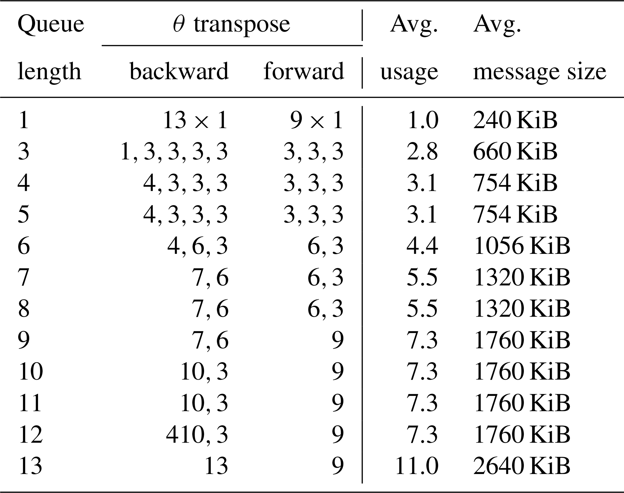
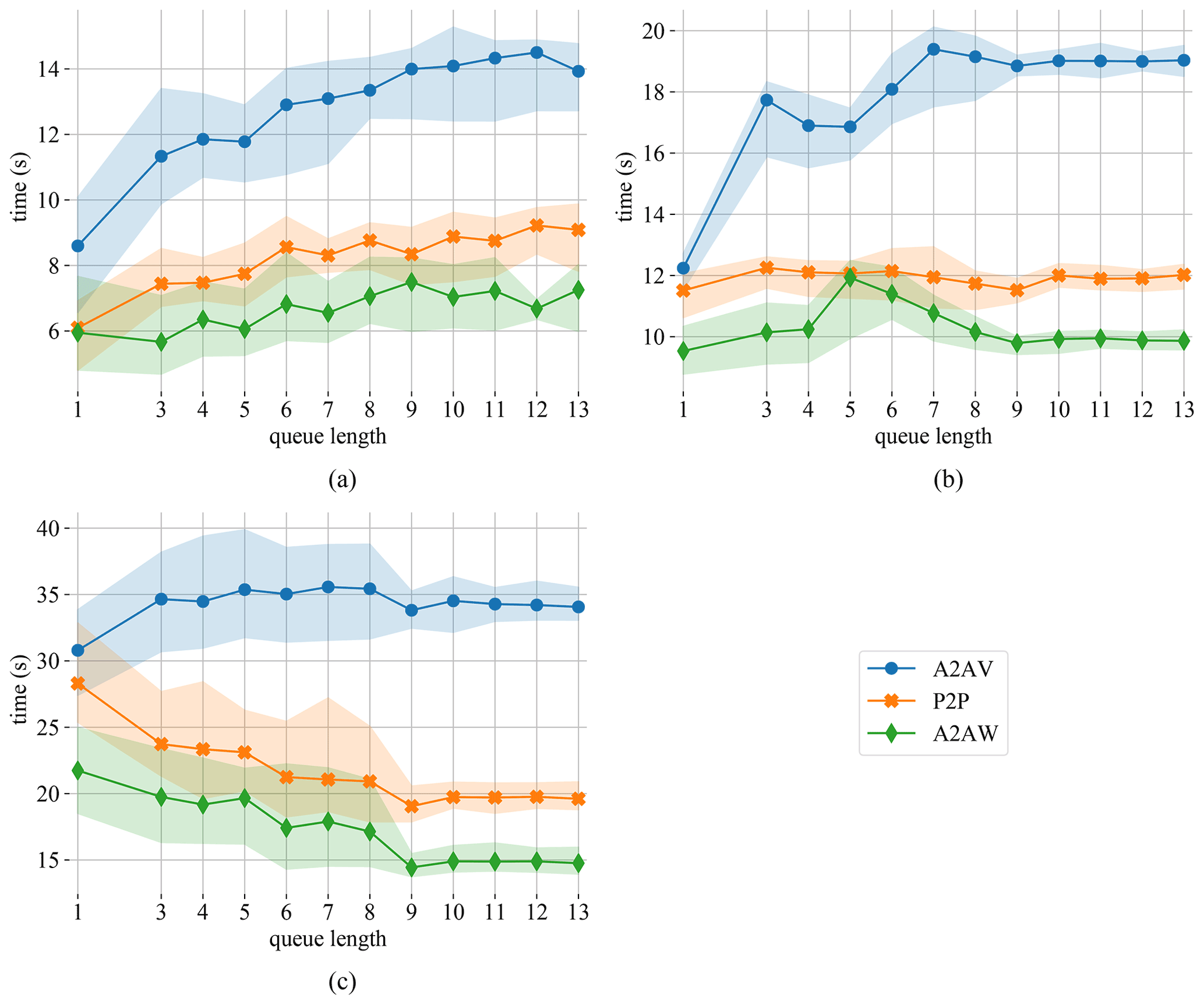
Figure 3Runtime for the θ transpose in the intranuma (a), intranode (b), and internode (c) regimes for varying queue length and 50 time steps.
Figure 3 shows the times for 50 time steps for the three different communication regimes. The inferior performance of the A2AV implementation is attributed to the time spent reordering the send and receive buffers. Both A2AW and P2P use the same MPI types to avoid this reordering and therefore perform very similar. Concerning the queue length, the intranuma and intranode regimes perform best with smaller queues, while the opposite is true for the internodes regime.
Since the A2AW implementation for the θ transposition seems to perform best, we stick to this scheme for the following test wherein we address the impact of the queue length.
4.2 2d-MPI SHT benchmark
In this subsection we continue the comparison between intranuma, internuma, and internode regimes but now bring the whole spherical harmonics transform into perspective. Since this constitutes one of the largest portions of the computation, it is particularly interesting to determine the behaviour in the different communication regimes.
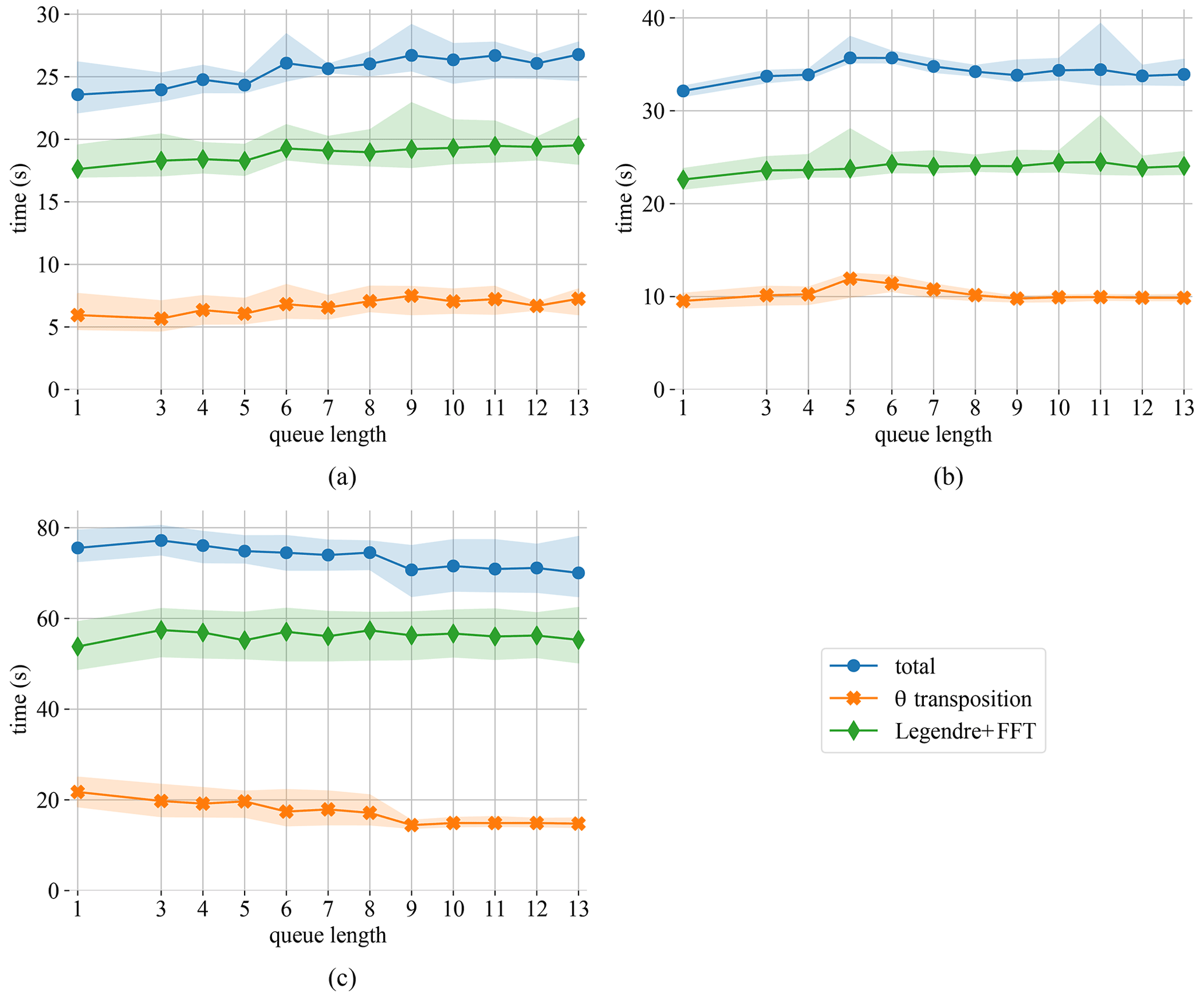
Figure 4Runtime for the different components of the SHT in the intranuma (a), intranode (b), and internode (c) regimes. Data are for 50 time steps using the A2AW implementation.
Figure 4 shows the θ-transposition time as well as the computation time spent inside the FFT and Legendre transform calls. Although the computation time itself should not depend on the queue length, Fig. 4 shows a small but consistent influence. We assume that this is linked to the change in data access pattern caused by queuing and buffering data for the θ transposition.
Even for the intranuma case shown in Fig. 4a, where a queue length of 3 provides a small performance boost for the θ transposition, the performance of the SHT is optimal for a queue length of 1. In the following test we therefore fix the queue length to 1 for intranuma and intranode regimes and to 13 for the internode regime.
4.3 The ℓ-transpose strong scaling benchmark
In this subsection we compare the performance of the four different ℓ-transposition implementations for the 2d-MPI version. We would like to recall that the 1d-hybrid implementation uses an auto-tuning routine which automatically selects the best algorithm during the initialization. Moreover, the main difference between 1d-hybrid and 2d-MPI implementations in the ℓ loop is the distribution of the (ℓ,m) tuples, as already discussed in Sect. 3.2. The communication pattern therefore differs significantly for the two implementations.
The problem we chose for this and subsequent subsections is the dynamo benchmark with Nr=301 and Nθ=960. We compute 100 time steps for several values of Πr and Πθ, as well as for core counts ranging from 120 to 24 000 (3 to 600 nodes, respectively). For the 1d-hybrid implementation, we use 10 OpenMP threads per MPI task for tests with up to 1000 cores (25 nodes) and 20 threads for larger runs (this configuration resulted in the best total time). The 1d-hybrid version of the code can use at most 6000 cores (150 nodes) with one radial point per socket (Πr=300 and 20 threads per MPI task).
For the 2d-MPI scheme, we fix the θ-transposition implementation to A2AW (as discussed in Sect. 4.1) and the queue lengths to 1 for Πθ=10, 20, or 40 and 13 otherwise. This new version of MagIC admits more combinations of Πθ and Πr and allows the use 24 000 cores (600 nodes). For some core counts, multiple values of Πθ and Πr were allowed. For example, for 6000 cores one may choose Πθ=20 or Πθ=40 with Πr=300 or Πr=150. We tested both and kept the configuration with the best total time. For the reader's convenience, all plots show the value of Πθ for the 2d-MPI version at the top horizontal axis. We also set the experiments such that Nr−1 is divisible by Πr and assign the last radial point to the last radial MPI rank. This is currently a limitation of MagIC. In principle, this should cause imbalance in some cases; e.g. with Πr=300 the last radial MPI rank will store and solve twice the number of radial levels as the other ranks. However, the last radial MPI rank receives fewer (ℓ,m) tuples, which diminishes the impact of the imbalance. Since both codes suffer from the same imbalance, we opt for simplifying the analysis to the average runtime only.
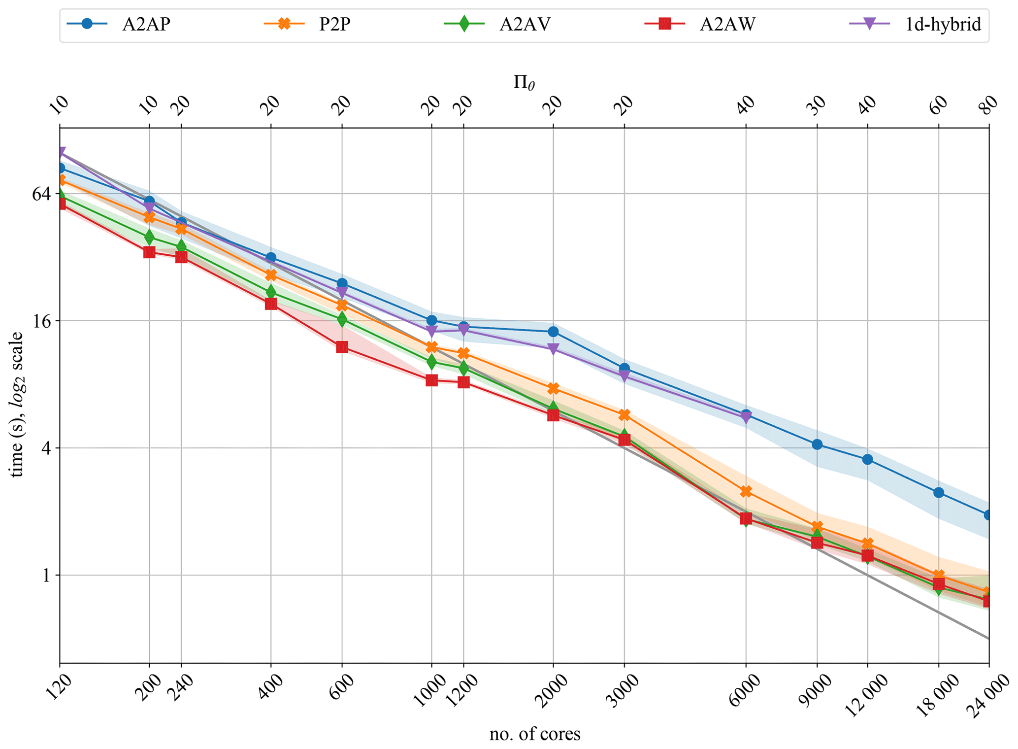
Figure 5Strong scalability of ℓ transposition for 100 time steps of the dynamo benchmark (Nr=301 and Nθ=960).
In Fig. 5 we can see that, except for the A2AP variant, the 2d-MPI implementation is always significantly faster than the 1d-hybrid implementation. This is a direct consequence of the communication-avoiding pattern of the 2d-MPI distribution.
The 1d-hybrid version shows a good strong scalability, which, however, starts to degrade after 1000 cores (25 nodes). At this core count the 1d-hybrid version transitions from 10 to 20 threads. OpenMP efficiency is typically difficult to maintain for large thread counts, and this is likely the reason for the performance degradation.
The 2d-MPI implementation, especially for the A2AW variant, scales remarkably well up to 6000 cores (150 nodes), at which point the performance starts to degrade. However, the losses remain acceptable up to the largest number of cores we could test: 24 000. The A2AV variant performs similarly to A2AW, and beyond 12 000 cores all variants show nearly identical timings. This test suggests preferring A2AW, which will be kept in the following. However, as the behaviour may be different on other architectures and for other MPI libraries, an auto-tuning routine that selects the fastest option in the initialization phase of a simulation seems a good idea for the future.
4.4 The ℓ-loop strong scaling
In this subsection we take a deeper look into the different parts of the ℓ loop. We are especially interested in the impact of the 2d-MPI data distribution on the LU decomposition and on the backward substitution. For these tests we use the same setting as in the previous subsection (100 time steps, Nr=301, and Nθ=960) and stick to the A2AW implementation of the transpositions.
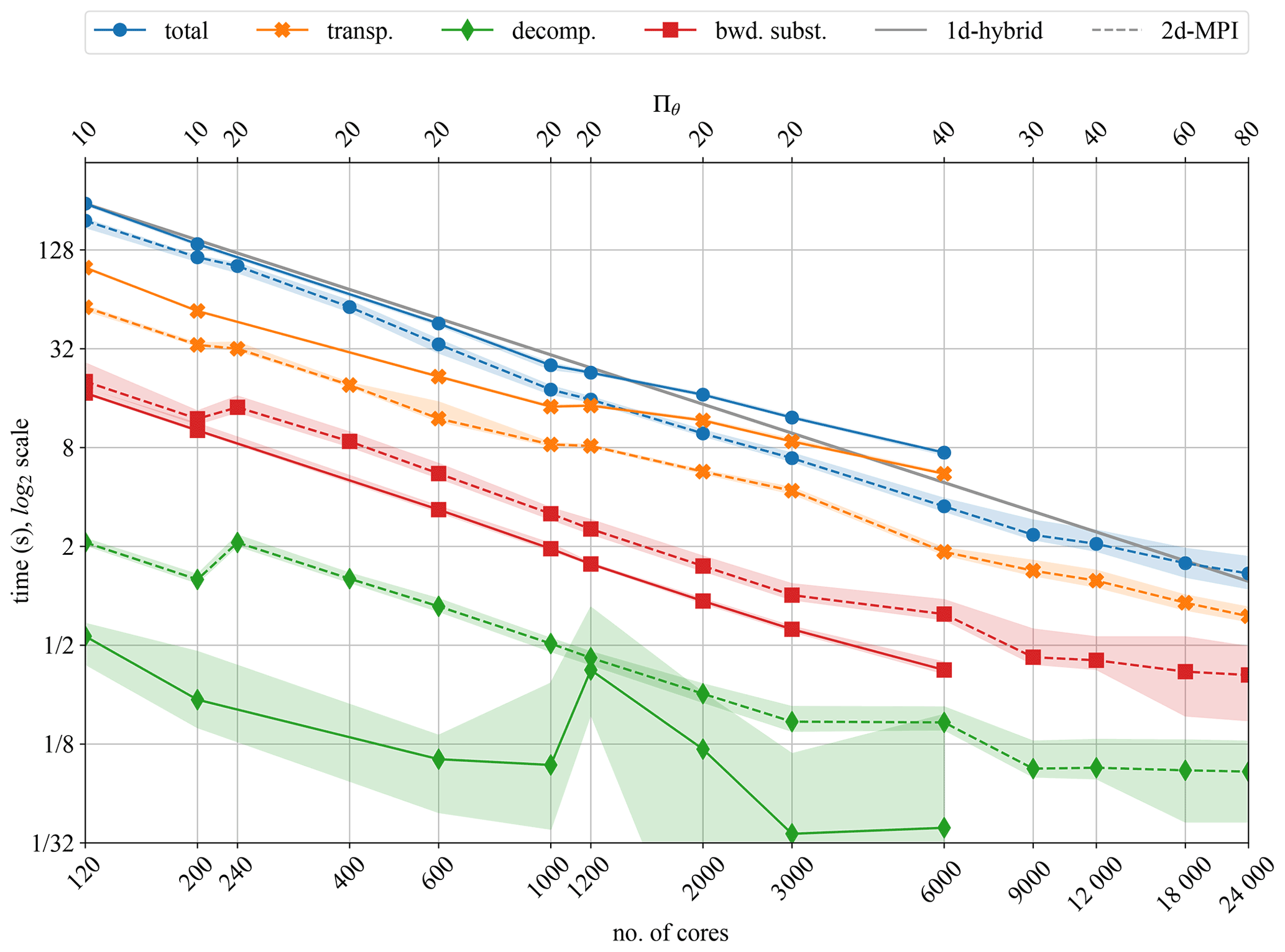
Figure 6Strong scalability for the ℓ transposition, LU decomposition, and backward substitution for the dynamo benchmark.
In Fig. 6 we compare transposition time, LU decomposition time, and the backward substitution time (referring to Eq. 19) for the 1d-hybrid and the 2d-MPI implementations. In addition, the total times for the ℓ loop are shown, which also include the updating of time derivatives and related operations.
In both the 1d-hybrid and 2d-MPI implementations, the performance is dominated by the transposition time. Here the 2d-MPI clearly outperforms the 1d-hybrid implementation because of the reduced communication, as discussed in Sect. 3.2.
The timing results in Fig. 6 demonstrate that decomposition and backward substitution for the linear systems do not scale well with Πθ (upper horizontal axis). As explained in Sect. 3.2, the data are distributed in the direction of the m modes, but the time-stepping matrices, which need to be LU-decomposed, are independent of m.
For a fixed Πr, the decomposition time is thus expected to remain independent of Πθ. Likewise, the backward substitution time should just mildly be impacted by larger Πθ. This can be clearly seen in Fig. 6: 120 and 240 cores have Πr=12, with Πθ=10 and 20, respectively. Their decomposition time is roughly the same, with a slightly faster backward substitution time for 240 cores. The same can be observed for 200 and 400 cores as well as 3000 and 6000 cores. There is a spike in the decomposition time for the 1d-hybrid implementation at 1200 cores.
However, the performance gain due to the communication-avoiding distribution of the 2d-MPI implementation far outweighs these shortcomings. We would like to highlight the fact that it is only possible to reduce the communication volume due to the particular distribution pattern shown in Fig. 2; i.e. each θ rank communicates with Πr ranks in the radial direction. The communication-avoiding scheme discussed here is not possible for the 1d-hybrid implementation, since one of these directions is missing. This specific feature of the 2d-MPI version is essential to enable a better overall performance for large cores count, as we shall discuss in the next subsection.
4.5 Overall performance and strong scaling comparison
Finally we discuss the strong scaling of the MagIC time step, i.e. of the main application without initialization, finalization, and diagnostics. As usual, we define the parallel efficiency as
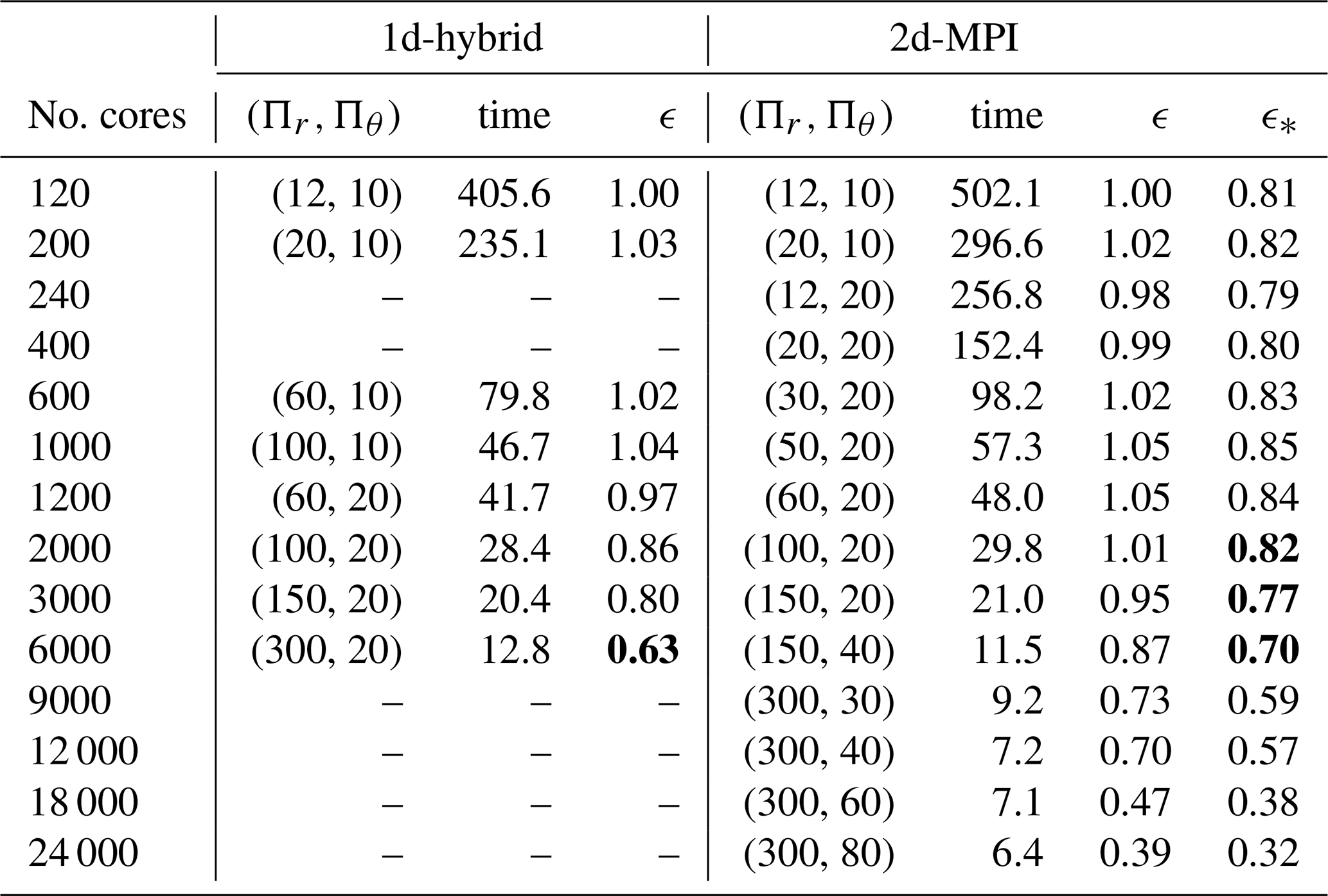
where t is the main application time in seconds and n is the number of cores used. We use the test with nref.=120 as a reference.
Following Matsui et al. (2016), we consider ϵ>0.6 to be a sufficiently good efficiency. Additionally, we define the “parallel cross-efficiency” ϵ* that compares the 2d-MPI timing to the 1d-hybrid reference time tref.=405.6 s for nref.=120 as a baseline. The timings and parallel efficiency, along with other information about the tests, are listed in Table 2. The graphical visualization of these values (also discriminating the time for the ℓ loop and radial loop) is shown in Fig. 7. Since we use the same problem size and settings already discussed in Sect. 4.3 and 4.4 the curves for the ℓ loop are the same as in Fig. 6.
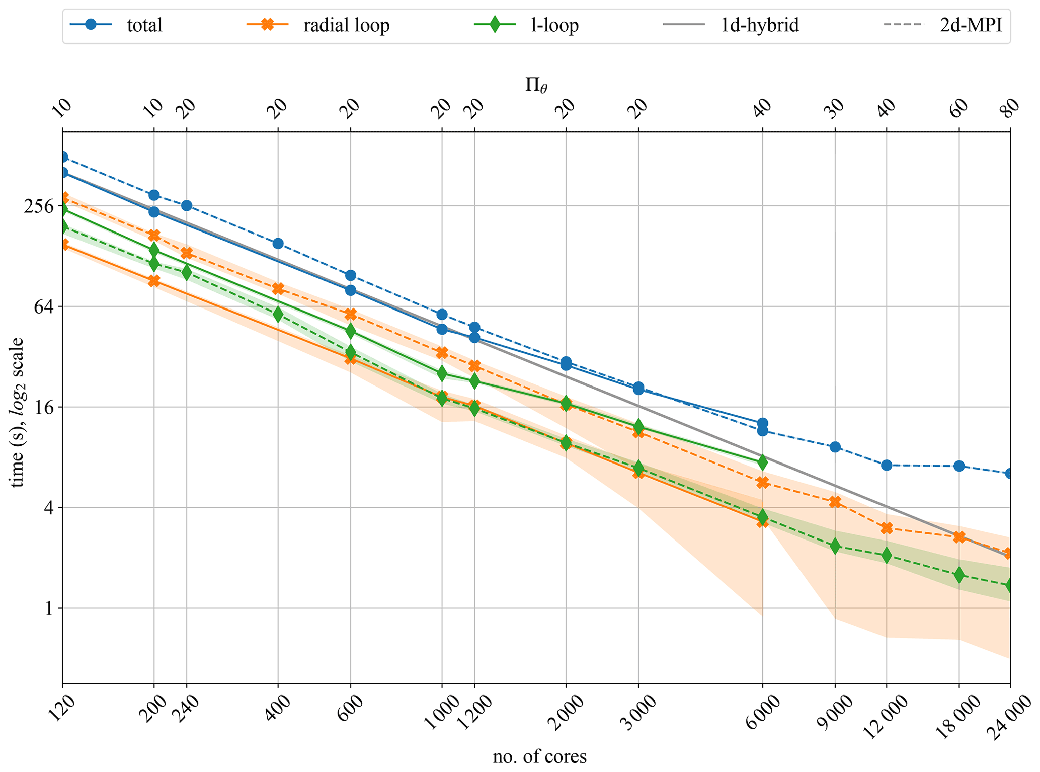
Figure 7Strong scalability for the 1d-hybrid and 2d-MPI implementations of MagIC for 100 time steps of the dynamo benchmark using Nr=301 and Nθ=960.
Table 2Parallel efficiency and cross-efficiency of the 1d-hybrid and 2d-MPI implementations, detailing Πr and Πθ as well as the main runtime in seconds. The bold font highlights values of interest.
In Fig. 7 it is interesting to notice that the performance of the 1d-hybrid implementation is dominated by the ℓ-loop performance, whereas the performance of the 2d-MPI implementation is dominated by the performance of the radial loop. To some degree this is expected because the radial loop of the 2d-MPI implementation requires the θ transposition in addition to the SHT.
The radial loop for the 1d-hybrid code scales well up to 6000 cores, but the inferior scalability of the ℓ loop already leads to a noticeable degradation beyond 1200 cores in Fig. 7. This is the cause of the decrease in parallel efficiency ϵ apparent in Table 2 for 2000 or more cores.
The 2d-MPI implementation starts suffering from a small loss of scalability of the ℓ loop at 9000 cores but remains at an acceptable level up to 24 000 cores. The radial loop scales remarkably well up to 12 000 cores but shows degraded performance at 18 000 and 24 000 cores. This can be explained by the problem size being too small for such numbers of cores, which is reflected by and for 9000 cores. Both the ℓ and the radial loop contribute to the loss of overall performance at the highest core counts apparent in Fig. 7.
The parallel cross-efficiency (see Table 2 and Fig. 7) shows that the new 2d-MPI version is about 20 % slower than the 1d-hybrid implementation for core counts of n<2000. However, the 2d-MPI variant scales better for n≥2000 with ϵ=0.7 for up to n=12 000. The 1d-hybrid implementation, on the other hand, reaches ϵ=0.63 for 6000 cores. The 2d-MPI is as fast as the 1d-hybrid implementation at n=3000 but already 10 % faster at n=6000.
The benefits offered by the 2d-MPI implementation can be illustrated with a simple example. Instead of performing a simulation with the 1d-hybrid implementation on 6000 cores a scientist could opt for using the 2d-MPI implementation on 12 000 cores and obtain the solution in only 56 % of the runtime. In other words, by investing only 12.5 % more CPU hours, the 2d-MPI implementation arrives at the same solution in half the time. Furthermore, using the 2d-MPI implementation allows the user to allocate more computing nodes and thus gives the user access to more distributed memory.
The parallel cross-efficiency also gives an idea of how “far” the parallel efficiency of the 2d-MPI is from the 1d-hybrid implementation. There is a significant gap for 120 to 1200 cores, but the gap closes at about 2000 cores, e.g. ϵ=0.86 for the 1d-hybrid and . This trend continues until 6000 cores, when the parallel cross-efficiency overtakes the parallel efficiency of the 1d-hybrid implementation.
Finally, the main characteristics measured on our benchmark platform are expected to be transferable to other flavours of HPC platforms based on contemporary x86_64 CPUs (e.g. AMD EPYC) and high-performance interconnects (e.g. Mellanox Infiniband), provided the platforms are sufficiently optimized for SHTns and MPI libraries. In general, for good performance of the 1d-hybrid version it is mandatory to establish the optimal number of threads per MPI rank and to respect the placement of the threads within the NUMA domains. The new 2d-MPI version brings the advantage of being less affected by the actual node topology, but the performance of the application is sensitive to the MPI library optimization of routines such as mpi_alltoallw for shared-memory environments.
4.6 Analysis of the radial loop
The parallel cross-efficiency in Table 2 shows that the performance of both implementations is rather close for core counts larger than 2000. This rightfully raises the question of whether this small gap could be bridged. Furthermore, it has already been established in previous sections that the main bottleneck of the 2d-MPI implementation is the radial loop, but the θ transposition and the computation time (i.e. mostly the SHT) of the radial loop have not yet been thoroughly compared. The goal of this subsection is to provide this comparison and discuss which portions of the code could be optimized and what impact this could have on the 2d-MPI implementation.
For the 1d-hybrid code, let tt and tr respectively denote the full time of the main application and the radial loop only, both given in seconds. Analogously, for the 2d-MPI code, let Tt denote the time of the full main application and Tr+Tθ denote the time of the radial loop only, where Tr is the computation time only and Tθ is the θ-transposition time only (including communication and necessary buffer copies, if any). Table 3 shows tr, Tr, and Tθ for the same experiment from 120 to 6000 cores. Both tt and Tt have the same values shown in the “time” columns of Table 2.
Table 3 shows that the θ-transposition times comprises on average 17.5 % of the radial loop (except for 6000 cores, for which it takes circa 28 % of the time of the radial loop). The runtime of θ transposition can be further optimized e.g. by introducing complex strategies such as communication–computation overlap. However, from Table 3 it is evident that the main bottleneck is indeed the computation time Tr.
The next natural question is how the computation times of the radial loop of both implementations compare with each other. For that we use the ratio
Ideally, ρ would be always close to 1, in which case the computational efficiency of the radial loop of both implementations would be identical. In practice, distributing the data between more MPI ranks means that each rank has less local data, which makes cache-hitting, vectorization, and other fine-grained optimization techniques less efficient. In other words, even a finely optimized implementation of the 2d-MPI data distribution algorithm is likely to have ρ>1.
The column ρ from Table 3 shows that the performance gap is far from 1 in most cases and is inversely proportional to the number of cores. This means that bridging the large gap in performance for the lower core counts might be unfeasible, but for larger core counts it is attainable.
Table 3Radial loop performance comparison for the dynamo benchmark. tt (Tt) is the main application time for the 1d-hybrid (2d-MPI) implementation. tr (Tr) is the computation time for the radial loop of the 1d-hybrid (2d-MPI) implementation, and Tθ is the time for the θ transposition in the 2d-MPI implementation. All times are given in seconds. The columns ρ and κ are defined in Eqs. (21) and (22), respectively.
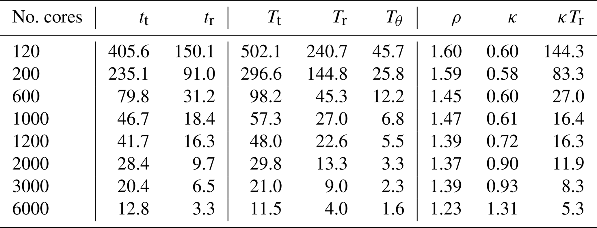
We now attempt to determine how much improvement in the 2d-MPI implementation is required for its main application runtime (including all transposition times) to match the runtime of the 1d-hybrid code. In practice, several portions of the 2d-MPI code could benefit from cache-hitting strategies, fine-tuned vectorization, and computation–communication overlap, amongst others. We will now discuss a much simpler scenario in which only the computation time of the radial loop can be improved from Tr to κTr. Subtracting Tr from the total time Tt and adding the “new” runtime κTr, we obtain the following equation:
which gives us the needed improvement factor κ. The values are shown in Table 3.
Table 3 shows that, for low core counts, improvements in Tr alone could not bridge the gap in the performance between 2d-MPI and the 1d-hybrid implementations. From 120 to 1000 cores we have tr>κTr, meaning that the 2d-MPI implementation would have to compute the radial loop faster than the already highly optimized 1d-hybrid code for both codes to perform the same.
The last three entries in Table 3 show a much more realistic improvement factor. An improvement of 10 % (7 %) in Tr would suffice to bridge the gap between the main application time for 2000 cores (3000 cores). For 6000 cores, Table 3 shows that Tr could be 31 % slower and both codes would still be equivalent. This is due to the poor scalability of the ℓ transposition of the hybrid code, which gives the 2d-MPI some “room” for performance loss in other portions of the code.
We described a new parallelization scheme based on a two-dimensional, MPI-based data decomposition for MagIC, an open-source code for three-dimensional fluid dynamics simulations in spherical geometry, with high scientific impact in a broad range of scientific fields ranging from fundamental fluid dynamics and modelling of planetary dynamos to stellar dynamics. MagIC uses spherical surface harmonics of degree ℓ and order m for the spectral representation in longitude and latitude and Chebyshev polynomials in radius. Our newly implemented 2d-MPI scheme is compared to the previously established 1d-hybrid code version that uses MPI and OpenMP and that has been highly optimized over years.
Thanks to a number of new concepts, the 2d-MPI version presented here can already compete with the hybrid parallelization in terms of runtime, and in addition it offers the possibility to use a significantly larger number of cores. It opens the possibility to employ tens of thousands of CPU cores on modern HPC clusters and paves the way to using the next-generation CPU architectures.
Decisive factors for its success include a communication-avoiding data distribution of the ℓ and m modes for the computation of the actual time step in MagIC and the optimization of the associated communications strategies. Compared to the existing one-dimensional data decomposition, the new two-dimensional data distribution scheme requires an additional costly transposition in the azimuthal direction. This leads to a performance penalty at low core counts which might be hard to overcome. However, for the dynamo benchmark and the setups considered here, and starting at moderate core counts of 2000, the performance of the new version is mostly limited by the not yet fully optimized main radial loop, which can be as much as 60 % slower than its counterpart in the one-dimensional data distribution.
Our results showed that a mere 10 % performance gain in the computation time of the radial loop of the 2d-MPI implementation would bridge the gap between the two code versions for 2000 cores or more, in addition to providing an extended strong scalability regime. Other sets of equations solved by MagIC, such as the anelastic equations (Jones et al., 2011), may present a different cost associated with the radial loop and would require a separate investigation.
Our implementation paves the way towards a future unified hybrid variant of MagIC which combines a two dimensional data distribution with the proven benefits of an additional OpenMP layer in order to further improve the computational performance across an even wider range of simulation scenarios. This future 2d-hybrid version could retain the benefits of our communication-avoiding data distribution and its improved strong scaling behaviour, while still benefiting from the performance of the finely optimized multithreaded libraries used within the radial loop. We expect that the performance of the radial loop of such a 2d-hybrid implementation will be closer to the performance of the 1d-hybrid version, effectively eliminating the main bottleneck of the 2d-MPI version.
Looking further into the future, the hybrid MPI-OpenMP parallelization of MagIC would be a natural starting point for developing a GPU-accelerated version of the code. Such a porting effort would probably start out from the 1d-hybrid version of MagIC, mapping an entire GPU to a radial zone (or MPI rank), and relying on the performance of the GPU variant of SHTns on top of the very high memory bandwidth and floating-point performance provided by an individual GPU of the current or next generation. A 2d-hybrid version of MagIC could serve as the basis for an even more flexible, accelerated version of MagIC e.g. for applications in which an even higher radial resolution is desired or when the individual accelerators (possibly of a kind different than GPU) are comparatively less powerful.
MagIC's source code is under active development and available for download from https://github.com/magic-sph/magic (last access: 24 June 2021) under the GNU GPL v3 license. The 1d-hybrid version discussed here is the commit c63930b of the master branch (version 5.10). A frozen version is archived on Zenodo (https://doi.org/10.5281/zenodo.5204425, Gastine et al., 2021). The 2d-MPI version is the commit 6cabfa7 of the merge-paral branch on GitHub, branched from commit c63930b. A frozen version has also been archived on Zenodo (https://doi.org/10.5281/zenodo.5171780, Lago et al., 2021).
No data sets were used in this article.
TG and JW developed and maintained the main branch of MagIC. TG also managed the use of external libraries (FFTW, LAPACK, SHTns, etc.) and fine optimization of OpenMP. TD conceptualized, implemented, and tested the algorithms for the 1d-hybrid implementation. RL conceptualized, implemented, and tested the algorithms for the 2d-MPI implementation. The numerical experiments were designed and conducted by RL with the supervision of TD and TG. TD and MR supervised HPC aspects of the project. JW and TG were responsible for supervising and interpreting the geophysical aspects of the project. The original draft was written by RL. The reviewing and editing of the current draft was conducted equally by all authors.
The contact author has declared that neither they nor their co-authors have any competing interests.
Publisher's note: Copernicus Publications remains neutral with regard to jurisdictional claims in published maps and institutional affiliations.
The article processing charges for this open-access publication were covered by the Max Planck Society.
This paper was edited by Josef Koller and reviewed by two anonymous referees.
Abramowitz, M. and Stegun, I. A.: Handbook of Mathematical Functions with Formulas, Graphs, and Mathematical Tables, Dover, New York, 9th dover printing, 10th gpo printing Edn., 1964. a
Anderson, E., Bai, Z., Bischof, C., Blackford, S., Dongarra, J. D. J., Croz, J. D., Greenbaum, A., Hammarling, S., McKenney, A., and Sorensen, D.: LAPACK Users' Guide, SIAM, Philadelphia, Pennsylvania, USA, 3rd Edn., 1999. a
Ascher, U. M., Ruuth, S. J., and Wetton, B. T. R.: Implicit-explicit methods for time-dependent partial differential equations, SIAM J. Numer. Anal., 32, 797–823, 1995. a
Ascher, U. M., Ruuth, S. J., and Spiteri, R. J.: Implicit-explicit Runge-Kutta methods for time-dependent partial differential equations, Appl. Numer. Math., 25, 151–167, 1997. a
Barik, A., Triana, S. A., Hoff, M., and Wicht, J.: Triadic resonances in the wide-gap spherical Couette system, J. Fluid Mech., 843, 211–243, https://doi.org/10.1017/jfm.2018.138, 2018. a
Boyd, J. P.: Chebyshev and Fourier spectral methods, Dover Publications, 2001. a, b
Breuer, M., Manglik, A., Wicht, J., Trümper, T., Harder, H., and Hansen, U.: Thermochemically Driven Convection in a Rotating Spherical Shell, Geophys. J. Int., 183, 150–162, https://doi.org/10.1111/j.1365-246X.2010.04722.x, 2010. a
Calypso: Calypso GitHub Page, GitHub [code], available at: https://github.com/geodynamics/calypso, last access: 24 June 2021. a
Christensen, U. and Wicht, J.: Numerical Dynamo Simulations, in: Core Dynamics, edited by: Olson, P., vol. 8 of Treatise on Geophysics, Elsevier, 2nd Edn., 245–277, 2015. a, b
Christensen, U. R., Aubert, J., Cardin, P., Dormy, E., Gibbons, S., Glatzmaier, G. A., Grote, E., Honkura, Y., Jones, C., Kono, M., Matsushima, M., Sakuraba, A., Takahashi, F., Tilgner, A., Wicht, J., and Zhang, K.: A numerical dynamo benchmark, Phys. Earth Planet. Int., 128, 25–34, https://doi.org/10.1016/S0031-9201(01)00275-8, 2001. a, b
Clune, T. C., Elliott, J. R., Miesch, M. S., Toomre, J., and Glatzmaier, G. A.: Computational aspects of a code to study rotating turbulent convection in spherical shells, Parallel Comput., 25, 361–380, 1999. a, b
Dormy, E., Cardin, P., and Jault, D.: MHD flow in a slightly differentially rotating spherical shell, with conducting inner core, in a dipolar magnetic field, Earth Planet. Sc. Lett., 160, 15–30, https://doi.org/10.1016/S0012-821X(98)00078-8, 1998. a
Featherstone, N.: Rayleigh 0.9.1, Zenodo [code], https://doi.org/10.5281/zenodo.1236565, 2018. a
Frigo, M. and Johnson, S. G.: The design and implementation of FFTW3, P. IEEE, 93, 216–231, 2005. a
Garcia, F., Net, M., García-Archilla, B., and Sánchez, J.: A comparison of high-order time integrators for thermal convection in rotating spherical shells, J. Comput. Phys., 129, 7997–8010, https://doi.org/10.1016/j.jcp.2010.07.004, 2010. a
Gastine, T. and Wicht, J.: Effects of Compressibility on Driving Zonal Flow in Gas Giants, Icarus, 219, 428–442, https://doi.org/10.1016/j.icarus.2012.03.018, 2012. a
Gastine, T., Yadav, R. K., Morin, J., Reiners, A., and Wicht, J.: From solar-like to antisolar differential rotation in cool stars, Mon. Not. R. Astron. Soc., 438, L76–L80, https://doi.org/10.1093/mnrasl/slt162, 2014. a
Gastine, T., Aubert, J., and Fournier, A.: Dynamo-based limit to the extent of a stable layer atop Earth’s core, Geophys. J. Int., 222, 1433–1448, https://doi.org/10.1093/gji/ggaa250, 2020. a
Gastine, T., Barik, A., rraynaud, t-schwaiger, Putigny, Bertrand, Wicht, J., thtassin, LDVDuarte, and Dintrans, B.: MagIV v5.10 (1d-hybrid) (5.10), Zenodo [code], https://doi.org/10.5281/zenodo.5204425, 2021. a
Glatzmaier, G. A.: Numerical Simulations of Stellar Convective Dynamos. I. the Model and Method, J. Comput. Phys., 55, 461–484, https://doi.org/10.1016/0021-9991(84)90033-0, 1984. a, b, c, d, e, f, g
Glatzmaier, G. A.: Introduction to modeling convection in planets and stars: Magnetic field, density stratification, rotation, Princeton University Press, 2013. a
Glatzmaier, G. A. and Roberts, P. H.: A three-dimensional convective dynamo solution with rotating and finitely conducting inner core and mantle, Phys. Earth Planet. Int., 91, 63–75, https://doi.org/10.1016/0031-9201(95)03049-3, 1995. a
Heimpel, M., Gastine, T., and Wicht, J.: Simulation of deep-seated zonal jets and shallow vortices in gas giant atmospheres, Nat. Geosci., 9, 19–23, https://doi.org/10.1038/ngeo2601, 2016. a
Hollerbach, R.: A Spectral Solution of the Magneto-Convection Equations in Spherical Geometry, Int. J. Numer. Meth. Fluids, 32, 773–797, https://doi.org/10.1002/(SICI)1097-0363(20000415)32:7<773::AID-FLD988>3.0.CO;2-P, 2000. a
Intel MKL: Developer Reference for Intel® oneAPI Math Kernel Library – C, available at: https://www.intel.com/content/www/us/en/develop/documentation/onemkl-developer-reference-c/top.html, last access: 1 December 2021. a
Ishioka, K.: A new recurrence formula for efficient computation of spherical harmonic transform, J. Meteorol. Soc. Jpn. Ser. II, 96, 241–249, 2018. a, b
Jones, C. A., Boronski, P., Brun, A. S., Glatzmaier, G. A., Gastine, T., Miesch, M. S., and Wicht, J.: Anelastic convection-driven dynamo benchmarks, Icarus, 216, 120–135, https://doi.org/10.1016/j.icarus.2011.08.014, 2011. a, b, c
Lago, R., Gastine, T., Wicht, J., Barik, A., rraynaud, t-schwaiger, Bertrand Putigny, thtassin, LDVDuarte, and Dintrans, B.: MagIC v5.10, commit 6cabfa7 (2d-MPI) (5.10), Zenodo [code], https://doi.org/10.5281/zenodo.5171780, 2021. a
Lantz, S. R. and Fan, Y.: Anelastic magnetohydrodynamic equations for modeling solar and stellar convection zones, ApJS, 121, 247–264, 1999. a
Livermore, P. W.: An implementation of the exponential time differencing scheme to the magnetohydrodynamic equations in a spherical shell, J. Comput. Phys., 220, 824–838, https://doi.org/10.1016/j.jcp.2006.05.029, 2007. a
MAG: MAG GitHub Page, GitHub [code], available at: https://github.com/geodynamics/mag, last access: 24 June 2021. a
MagIC: MagIC GitHub Page, GitHub [code], available at: https://github.com/magic-sph/magic, last access: 24 June 2021. a
Marti, P. and Jackson, A.: A fully spectral methodology for magnetohydrodynamic calculations in a whole sphere, J. Comput. Phys., 305, 403–422, https://doi.org/10.1016/j.jcp.2015.10.056, 2016. a, b
Marti, P., Schaeffer, N., Hollerbach, R., Cébron, D., Nore, C., Luddens, F., Guermond, J. L., Aubert, J., Takehiro, S., Sasaki, Y., Hayashi, Y. Y., Simitev, R., Busse, F., Vantieghem, S., and Jackson, A.: Full sphere hydrodynamic and dynamo benchmarks, Geophys. J. Int., 197, 119–134, https://doi.org/10.1093/gji/ggt518, 2014. a
Marti, P., Calkins, M. A., and Julien, K.: A computationally efficient spectral method for modeling core dynamics, Geochem. Geophy. Geosy., 17, 3031–3053, https://doi.org/10.1002/2016GC006438, 2016. a, b
Matsui, H., King, E., and Buffett, B.: Multiscale convection in a geodynamo simulation with uniform heat flux along the outer boundary, Geochem. Geophy. Geosy., 15, 3212–3225, https://doi.org/10.1002/2014GC005432, 2014. a
Matsui, H., Heien, E., Aubert, J., Aurnou, J. M., Avery, M., Brown, B., Buffett, B. A., Busse, F., Christensen, U. R., Davies, C. J., Featherstone, N., Gastine, T., Glatzmaier, G. A., Gubbins, D., Guermond, J.-L., Hayashi, Y.-Y., Hollerbach, R., Hwang, L. J., Jackson, A., Jones, C. A., Jiang, W., Kellogg, L. H., Kuang, W., Landeau, M., Marti, P., Olson, P., Ribeiro, A., Sasaki, Y., Schaeffer, N., Simitev, R. D., Sheyko, A., Silva, L., Stanley, S., Takahashi, F., Takehiro, S.-i., Wicht, J., and Willis, A. P.: Performance Benchmarks for a next Generation Numerical Dynamo Model, Geochem. Geophy. Geosy., 17, 1586–1607, https://doi.org/10.1002/2015GC006159, 2016. a, b, c, d, e
Olson, P., Christensen, U., and Glatzmaier, G. A.: Numerical modeling of the geodynamo: Mechanisms of field generation and equilibration, J. Geophys. Res., 104, 10383–10404, https://doi.org/10.1029/1999JB900013, 1999. a
Orszag, S. A.: On the Elimination of Aliasing in Finite-Difference Schemes by Filtering High-Wavenumber Components, J. Atmos. Sci., 28, 1074–1074, https://doi.org/10.1175/1520-0469(1971)028<1074:OTEOAI>2.0.CO;2, 1971. a
Press, W. H., Flannery, B. P., Teukolsky, S. A., and Vetterling, W. T.: Numerical Recipes: The art of scientific computing, vol. 1, Cambridge University Press, 3rd Edn., 2007. a
Rayleigh: Rayleigh GitHub Page, GitHub [code], available at: https://github.com/geodynamics/rayleigh, last access: 24 June 2021. a
Raynaud, R., Guilet, J., Janka, H.-T., and Gastine, T.: Magnetar formation through a convective dynamo in protoneutron stars, Sci. Adv., 6, eaay2732, https://doi.org/10.1126/sciadv.aay2732, 2020. a
Schaeffer, N.: Efficient Spherical Harmonic Transforms Aimed at Pseudospectral Numerical Simulations, Geochem. Geophy. Geosy., 14, 751–758, https://doi.org/10.1002/ggge.20071, 2013. a, b, c, d
Schaeffer, N., Jault, D., Nataf, H. C., and Fournier, A.: Turbulent geodynamo simulations: a leap towards Earth's core, Geophys. J. Int., 211, 1–29, https://doi.org/10.1093/gji/ggx265, 2017. a
SHTns: SHTns Bitbucket Page, GitHub [code], available at: https://bitbucket.org/nschaeff/shtns, last access: 24 June 2021. a, b
Takahashi, F.: Implementation of a high-order combined compact difference scheme in problems of thermally driven convection and dynamo in rotating spherical shells, Geophys. Astro. Fluid, 106, 231–249, https://doi.org/10.1080/03091929.2011.565337, 2012. a
Tassin, T., Gastine, T., and Fournier, A.: Geomagnetic semblance and dipolar–multipolar transition in top-heavy double-diffusive geodynamo models, Geophys. J. Int., 226, 1897–1919, https://doi.org/10.1093/gji/ggab161, 2021. a
Terra-Nova, F. and Amit, H.: Magnetic boundary layers in numerical dynamos with heterogeneous outer boundary heat flux, Phys. Earth Planet. Int., 309, 106589, https://doi.org/10.1016/j.pepi.2020.106589, 2020. a
Tilgner, A.: Spectral Methods for the Simulation of Incompressible Flows in Spherical Shells, Int. J. Numer. Meth. Fl, 30, 713–724, https://doi.org/10.1002/(SICI)1097-0363(19990730)30:6<713::AID-FLD859>3.0.CO;2-Y, 1999. a
Wicht, J.: Inner-core conductivity in numerical dynamo simulations, Phys. Earth Planet. Int., 132, 281–302, https://doi.org/10.1016/S0031-9201(02)00078-X, 2002. a, b
Wicht, J.: Flow instabilities in the wide-gap spherical Couette system, J. Fluid Mech., 738, 184–221, https://doi.org/10.1017/jfm.2013.545, 2014. a
XSHELLS: XSHELLS Bitbucket Page, GitHub [code], available at: https://bitbucket.org/nschaeff/xshells/, last access: 24 June 2021. a