the Creative Commons Attribution 4.0 License.
the Creative Commons Attribution 4.0 License.
 | 02 Dec 2021
Machine-learning models to replicate large-eddy simulations of air pollutant concentrations along boulevard-type streets
Moritz Lange
Henri Suominen
Mona Kurppa
Leena Järvi
Emilia Oikarinen
Rafael Savvides
Running large-eddy simulations (LESs) can be burdensome and computationally too expensive from the application point of view, for example, to support urban planning. In this study, regression models are used to replicate modelled air pollutant concentrations from LES in urban boulevards. We study the performance of regression models and discuss how to detect situations where the models are applied outside their training domain and their outputs cannot be trusted. Regression models from 10 different model families are trained and a cross-validation methodology is used to evaluate their performance and to find the best set of features needed to reproduce the LES outputs. We also test the regression models on an independent testing dataset. Our results suggest that in general, log-linear regression gives the best and most robust performance on new independent data. It clearly outperforms the dummy model which would predict constant concentrations for all locations (multiplicative minimum RMSE (mRMSE) of 0.76 vs. 1.78 of the dummy model). Furthermore, we demonstrate that it is possible to detect concept drift, i.e. situations where the model is applied outside its training domain and a new LES run may be necessary to obtain reliable results. Regression models can be used to replace LES simulations in estimating air pollutant concentrations, unless higher accuracy is needed. In order to have reliable results, it is however important to do the model and feature selection carefully to avoid overfitting and to use methods to detect the concept drift.
- Article
(4930 KB) - Full-text XML
-
Supplement
(995 KB) - BibTeX
- EndNote


Exposure to ambient air pollution leads to cardiovascular and pulmonary diseases, and is estimated to cause 3 million premature deaths worldwide every year (Lelieveld et al., 2015; WHO, 2016), of which 0.8 million occur in Europe (Lelieveld et al., 2019). Urban areas are generally characterized not only by high population densities but also higher air pollutant concentration levels compared to rural areas. The degraded air quality particularly in street canyons results from high local emissions, such as traffic combustion near the ground, as well as limited dispersion of these traffic-related pollutants. Streets with traffic are generally flanked with buildings and/or vegetation that inhibit pollutant ventilation upwards from the pedestrian level. Namely, dispersion is the main factor determining air quality (e.g. Kumar et al., 2011). Furthermore, these obstacles block, decelerate and modify air flow, leading to a highly turbulent wind field and pollutant dispersion patterns (Britter and Hanna, 2003). Consequently, certain urban planning solutions can be applied to enhance air pollutant dispersion and hence to improve local air quality to some extent (see, e.g. Kurppa et al., 2018; Nosek et al., 2016; Yuan et al., 2014). This, on the other hand, evokes the need for high-resolution, building-resolving air pollution modelling.
Successful modelling of urban air pollutant dispersion necessitates taking into account the detailed properties of adjacent buildings and vegetation in the area of interest as well as in its surroundings. To date, high-resolution dispersion modelling has mainly been based on physical modelling techniques, of which computational fluid dynamics (CFD) models, notably Reynolds-averaged Navier–Stokes (RANS) equations and large-eddy simulation (LES), are the most applicable tools for the purpose. CFD models solve the flow and dispersion around individual buildings, and with constantly increasing computational resources the modelling domains can currently be extended to cover entire neighbourhoods and even cities (Auvinen et al., 2020). However, conducting reliable and high-quality CFD simulations requires expertise in model application. Moreover, for building-resolving simulations that apply a grid resolution of 2 m or finer, especially LES necessitates supercomputing resources. At the same time, LES has been found more accurate than RANS in solving finer-scale details (Salim et al., 2011; Tominaga and Stathopoulos, 2011) and therefore particularly suitable in modelling flow and pollutant concentrations within real urban environments. In contrast to CFD, statistical models based on machine learning may offer a significantly less expensive alternative to predict urban air quality and pollutant dispersion. Consequently, the number of studies conducting machine-learning-based air quality modelling has increased rapidly (Rybarczyk and Zalakeviciute, 2018).
Machine learning allows finding a relationship between a target variable, e.g. the concentration of air pollutants in a certain location, and its predictors, which are often called features. These types of machine-learning models are called regression models. The models are trained on a specified training data which by some rule, e.g. maximizing the likelihood given that the relationship is linear with normally distributed noise, observe a relationship between the target variable and its features. To evaluate the trustworthiness of the results, often a part of the available data is not used to train the model but to evaluate it. These “unseen” evaluation data give an estimate of the model performance in a realistic urban planning scenario. Perhaps the largest advantage of regression models compared to the CFD models is their speed. However, the increase in speed comes at a cost of accuracy. Another disadvantage is that accurate predictions require the predicted data to follow approximately the same distribution as the training data, reducing their use to only modelling setups similar to those that they have been trained in.
Most of the previous studies on developing a statistical air pollution model using machine learning have been based on field measurements, and the spatiotemporal distribution of pollutants has been assessed by utilizing multiple stationary sites in model training (e.g. Araki et al., 2018; Yang et al., 2018). To further improve the spatial resolution of modelling in urban areas, also mobile air quality measurements have been utilized (e.g. Adams and Kanaroglou, 2016; Hu et al., 2017; Krecl et al., 2019; Van den Bossche et al., 2018). However, due to spatial accuracy constraints, the spatial resolution applied has been limited to the order of 10–50 m, which does not allow investigating the impact of individual buildings on pollutant dispersion. Output data from a numerical model have been used for training but only in the regional scale with a 5–15 km resolution (Feng et al., 2019; Peng et al., 2017). Machine-learning studies applying LES data have so far been mainly restricted to turbulence closure modelling (e.g. King et al., 2018).
In this study, the application of machine learning for emulating LES outputs of local-scale air pollutant dispersion in urban areas is investigated. We use LES outputs from two different studies conducted in different boulevard-type street canyons in Helsinki. Specifically, we create appropriate features for the neighbourhoods around the street canyons from the inputs of the LES that are used to train the machine-learning models and then evaluate the performance and reliability of different algorithms. The motivation is to approximate the computationally expensive simulations with machine-learning models that are faster to evaluate. The ultimate goal is to develop a model that can easily be applied to support urban planning.
This study is structured as follows: first, the LES datasets and feature construction are described. Then brief descriptions of the used machine-learning models and the training and evaluation process are provided. Finally, the applications, limitations and future work are discussed.
In this chapter, we introduce the LES datasets used in this study and explain our pre-processing steps. Then, we present the features available to the regression models. Finally, we describe how the optimal set of features is chosen by forward feature selection and describe the used performance measures. All analyses were carried out in R version 3.6.2 (R Core Team, 2020).
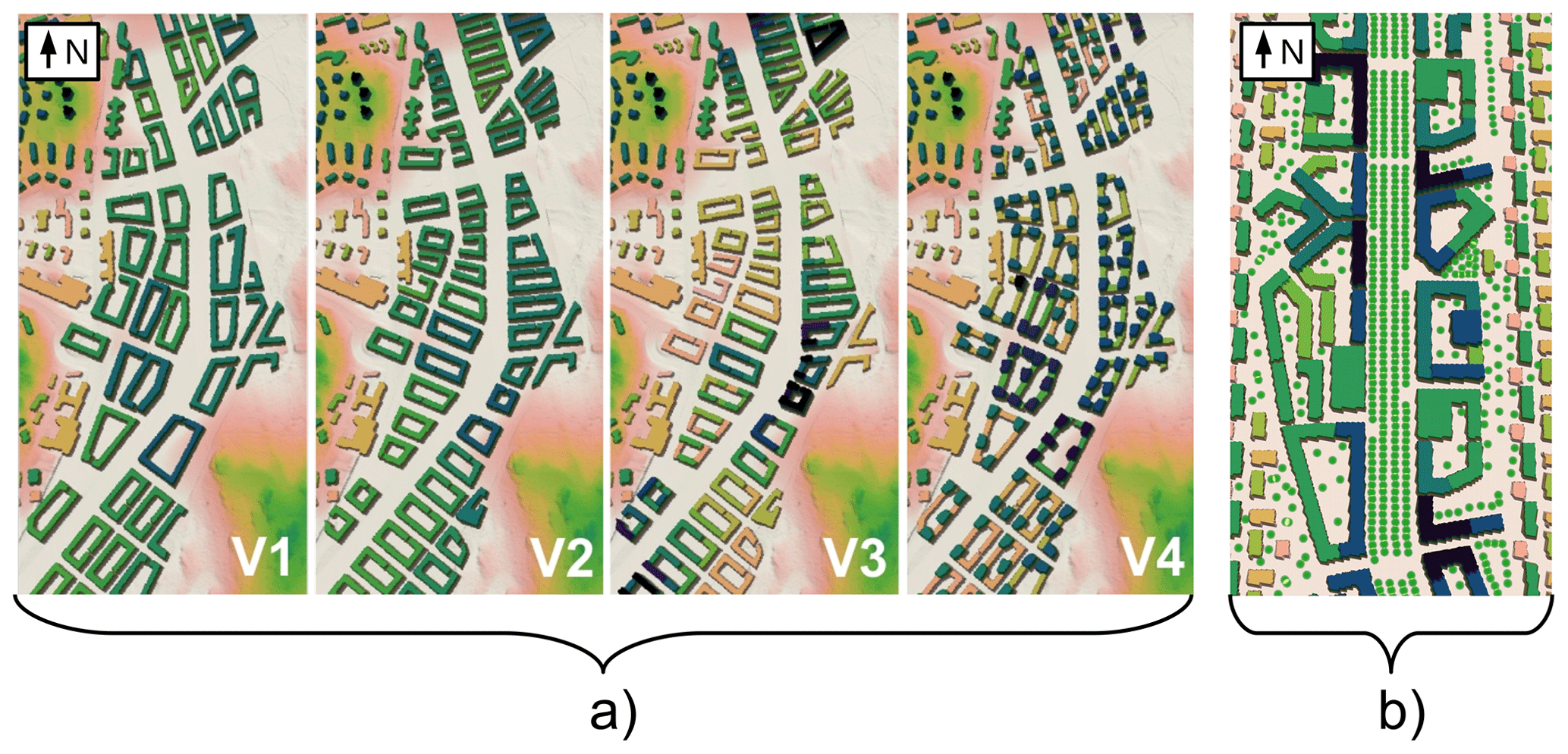
Figure 1Simulation domains of the LES output data applied in the study: (a) four city-planning alternatives (V1–V4) investigated in KU18 (Kurppa et al., 2018) and (b) city-boulevard scenario S1 and its surroundings studied in KA20 (Karttunen et al., 2020). Green dots illustrate trees. The city boulevard is 54 and 58 m wide in KU18 and KA20, respectively.
2.1 Large-eddy simulation datasets
LES models resolve the three-dimensional prognostic equations for momentum and scalar variables. In LES, all turbulence scales larger than a chosen filter width are resolved directly. The smaller scales, which should represent less than 10 % of the turbulence energy (Heus et al., 2010), are parameterized using a subgrid-scale model. This study uses output data from two studies to train and evaluate the regression methods: Kurppa et al. (2018) and Karttunen et al. (2020). Both studies apply the LES model PALM (Maronga et al., 2015, 2020) to assess the impact of city planning on the pedestrian-level air quality.
The first study by Kurppa et al. (2018, model revision 1904, hereafter KU18) investigates the impact of city-block orientation and variation in the building height and shape on the dispersion of traffic-related air pollutants. Specifically, LES is run over a 54 m-wide city boulevard applying four alternative city-planning solutions (V1–V4 in Fig. 1a). Here, simulations with a neutral atmospheric stratification and wind from east (90∘) and south-west (225∘) are considered. Air pollutant dispersion is studied by a Lagrangian particle model embedded in PALM. Air pollutants are represented as inert particles that are released above streets with traffic and follow the air flow without interacting with any surface. In the present study, 40 min averaged concentration fields from KU18 are employed.
The second study by Karttunen et al. (2020, model revision 3698, hereafter KA20) assesses the impact of street-tree layout on the concentrations of traffic-related aerosol particles. The study is conducted over a 50 to 58 m-wide city boulevard (Fig. 1b) with neutral atmospheric stratification under the two wind directions: parallel and perpendicular to the boulevard. Contrary to KU18, aerosol particle concentrations and size distributions as well as aerosol dry deposition on surfaces and vegetation are explicitly modelled by applying an aerosol module embedded in PALM (Kurppa et al., 2019). The aerosol module applies the Eulerian approach. Here, 1 h averaged concentration fields of PM2.5 (particulate matter with aerodynamic diameter <2.5 µm) for one modelling scenario (S1) are applied.
Both studies apply a grid spacing of 1.0 m in horizontal and 0.75–1.0 m in vertical to directly resolve the most relevant turbulent structures related to buildings and vegetation. The surface description is given to PALM by maps: namely those of topography elevation, tree height and emission strength per area. The simulations were conducted in a supercomputing environment and each simulation took approximately 103 d of CPU time.
The machine-learning models in this study are trained with KU18 and evaluated with KA20. Using KA20 for evaluation mimics a realistic urban planning scenario, where KA20 would correspond to a new city plan considered by the urban planner. KU18 is selected as the training dataset due to greater variety in building layouts compared to KA20, in which the variation is mainly limited to different street-tree scenarios. Clear differences in the building layouts lead to deviant pollutant dispersion and concentration distributions, which improves the generalization performance. An alternative approach for training would entail creating training and evaluation data using random samples from both KU18 and KA20. However, random sampling is impractical in this case due to significant differences between KU18 and KA20. KU18 simulates dispersion qualitatively and assumes weightless and inert particles that imitate air pollutants in general. In contrast, KA20 models realistic aerosol particle concentration values and includes realistic model physics for the aerosol dry deposition. These differences affect the scaling and distributions of the simulated particle concentrations (Fig. 2), which is further discussed in Sect. 3.2 and 3.3.
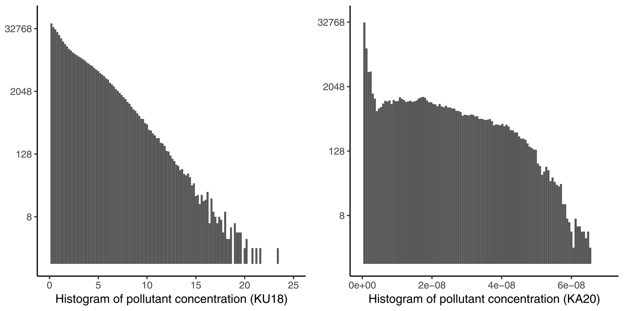
Figure 2Histograms of air pollutant concentrations in KU18 and KA20. Note the log scale of the counts on the y axis and the differing scales on the x axis. KA20 has units kg m−3.
2.2 Data pre-processing
The LES outputs KU18 and KA20 are pre-processed into a suitable format for training the regression models. The pre-processing is divided into two parts: aggregating the target variable over time and height, and constructing expressive features from the LES inputs.
2.2.1 Target variable
In regression, the target variable is predicted using predictor variables (features). Here, the target variable is the (air) pollutant concentration pc. The raw LES outputs contain pc on a spatiotemporal grid . We pre-process the target variable by averaging pc over time and considering a fixed height (at which pollutants are emitted). Then, pc values are predicted on the (x,y) grid instead of the grid. This simplifies the modelling task significantly while still retaining the relevant information on pc at the pedestrian level.
In addition to time averaging, we also restrict the spatial extent in which the regression models are trained. The area of interest in this study is the city boulevard in the middle of the maps, which is the same as in the original studies that generated KU18 and KA20. In KA20, the boulevard is surrounded by artificial buildings to imitate the aerodynamic roughness of an suburban environment, which however are of no interest and are therefore omitted in the model development. Figure 3 presents the exact areas used for modelling. The spatiotemporal aggregate is calculated by temporally averaging the LES data for the first 100 s displaying stable behaviour. Furthermore, only one vertical level is considered: 4 and 0.88 m above ground level for KU18 and KA20, respectively. This exact vertical level is chosen since it is the one at which the studied air pollutants are released in their respective simulations. In order to make the datasets more comparable, the background concentrations in KA20 are removed using the transformation pcnew =.
2.2.2 Features
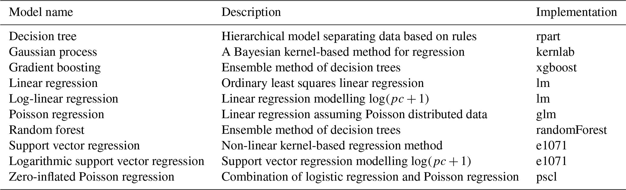
The target variable is predicted using features that are defined for each 1 m×1 m surface pixel in the modelling domain. The features include direct inputs to the LES and surrogate features which are constructed from these inputs. The direct LES inputs are “height of the topography”, which includes solid obstacles such as buildings, “height of the canopy” and “amount of pollutant emissions”. The features used for training the regression models are described briefly in Table 1 and in more detail in Table A1.
The surrogate features provide information about spatial dependencies in the modelling domain, reducing the need for the regression models to explicitly model these dependencies. For instance, applying convolutions of various sizes on pollutant emissions creates surrogate features of average pollutant emission densities over a spatial neighbourhood, weighted by proximity to the point in question. Other features, such as the height-to-width ratio of a street canyon, are created based on domain knowledge. Incorporating domain knowledge is important, since well-crafted input features largely determine the quality of modelling results. Furthermore, understandable features aid experts in interpreting the physical meaning of the results.
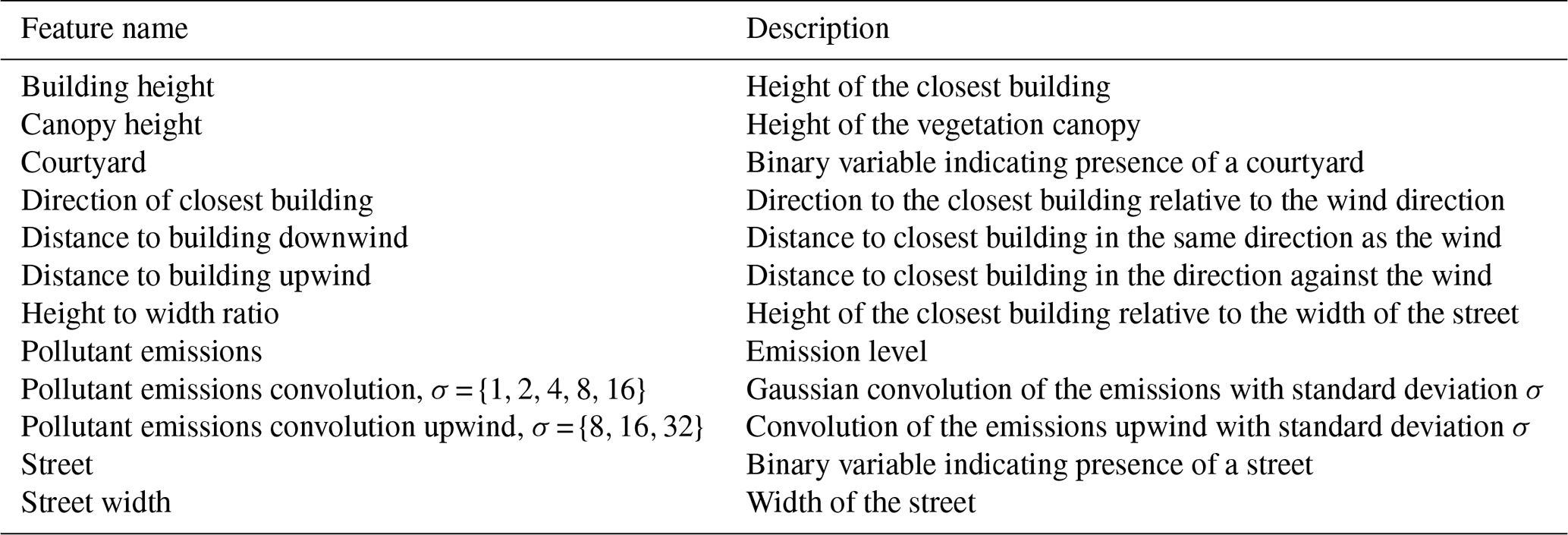
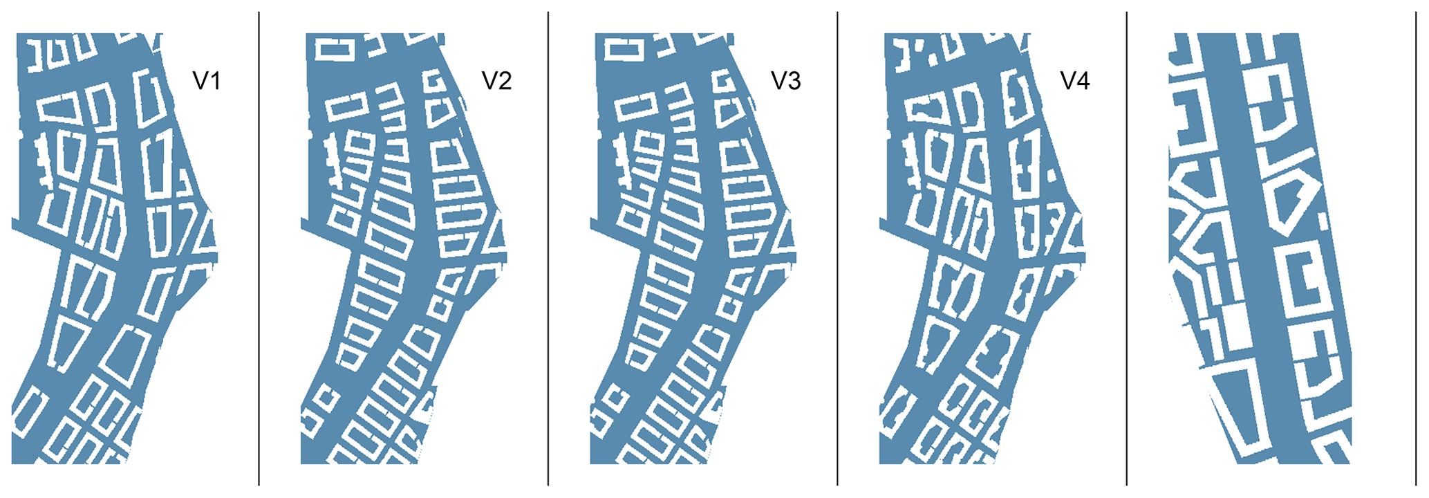
Figure 3The map area cutout for which pollutant concentrations are modelled (in blue) for each of the city plans (V1–V4) from Kurppa et al. (2018) and for the map area from Karttunen et al. (2020) (rightmost picture).
2.3 Forward feature selection
After calculating all potentially useful input features, a subset of features to be used with each model is selected using forward selection (Hastie et al., 2009). Forward selection is a feature selection algorithm in which a model is trained iteratively with progressively larger feature subsets. Initially, every feature is used as a single predictor to train the model, and the best-performing feature is selected. The model is then re-trained using this feature along with every other feature as a second predictor, and the second-best-performing feature is selected. This process is repeated until either all features are selected or no additional feature improves the model. Forward selection limits the search space of all possible feature combinations considerably, and while it does not guarantee to find the globally best subset of features, it finds a local optimum. An advantage of forward selection that is relevant to this study is that it avoids selecting strongly correlated predictors, such as the different-sized convolutions of pollutant emissions (Table 1).
The best-performing features are selected according to a selection criterion. Here, the selection criterion is the cross-validation root mean squared error (RMSE). Cross-validation is a technique for evaluating generalization performance of statistical models and for detecting overfitting. In cross-validation, the data are split into k random subsets, out of which k−1 are used to train the model, and one is used to validate the model. Due to the spatial auto-correlation in the LES data, a random split by sampling data points from all maps does not lead to statistically independent subsets. In order to ensure maximal independence between the training and validation data, the random split is performed at the level of city blocks. Each cross-validation split is trained with three different city plans under a given wind direction and validated with the fourth city plan under the other wind direction. This is repeated for all four city plans using both wind directions. As an example, one split uses city plans V1, V2 and V3 with the wind direction 90∘ as training data and V4 with a wind direction of 225∘ as validation data to validate predictions. Using each city plan for a given wind direction as unique validation data results in eight splits. The aggregated cross-validation error is then calculated as the error of all combined predictions of all splits.
Table 2Models and their implementation in R (version 3.6.2.) with all but two model pollutant concentrations (pc). For log-linear regression and logarithmic support vector regression, the model internally estimates log(pc+1), where +1 is added because of the zero values contained within pc. The predictions are transformed back to the original scale after being computed.
2.4 Model descriptions
The applicability of 10 common regression models trained on KU18 is examined, from the simplest linear model to the powerful support vector regression (SVR) model (Table 2).
- Linear models
-
Four generalized linear models are considered: linear regression, log-linear regression (Benoit, 2011), Poisson regression and zero-inflated Poisson regression (Lambert, 1992). Generalized linear models model the target variable as a function of linear combinations of features. Linear models are relatively simple, which limits their flexibility but makes them more interpretable. For example, if the features are normalized, then the regression coefficient of a feature communicates how much a change of one unit affects the mean of the target variable, given that all other features are constant.
- Tree-based models
-
Three tree-based models are considered: decision trees, random forest and gradient boosting with decision trees (Hastie et al., 2009). Decision trees model the target variable using simple if–else rules, which makes them interpretable. Random forest is an ensemble method that aggregates the predictions of multiple decision trees trained on random subsets of data and features. Gradient boosting is also an ensemble method in which multiple decision trees are trained sequentially on the results of previous trees, correcting their weaknesses. Ensemble methods achieve high prediction accuracy by pooling the predictions of multiple models. In particular, the random forest is among the best-performing regression models (Fernández-Delgado et al., 2014). However, the complexity of ensemble models means that they are not interpretable.
- Support vector regression
-
SVR (Cristianini and Shawe-Taylor, 2000) is a powerful regression method that implicitly transforms the data into a higher-dimensional feature space. This enables SVR to model interactions and conditional dependencies between features and hence utilize more information compared to simpler models. However, as with the complex tree models, the complexity of SVR leads to difficulties in understanding how the relations in the data are utilized by the model to estimate pc. In addition to standard SVR, a log-transformed SVR (log-SVR) is also used to enforce positive predictions for pc.
- Gaussian process regression
-
GPR (Murphy, 2012) is a non-parametric approach to regression. GPR is a Bayesian method that uses a Gaussian process with a known covariance as a prior to infer the posterior predictive distribution of the unobserved values. It can be considered as a Bayesian alternative for other kernel methods, such as SVR (Murphy, 2012). We use a squared exponential kernel as the covariance matrix for the model. This results in points having similar predicted values if they are close to each other in the feature space. The generally good performance of the GPR is also complemented by its built-in ability to account for uncertainty.
- Dummy model
-
A dummy model is used as a baseline model for reference. The dummy model simply predicts mean pc of the training data, regardless of any features.
2.5 Performance measure
The RMSE is a standard performance measure for model evaluation (Rybarczyk and Zalakeviciute, 2018). Here, a modified version of RMSE is used, due to the different scales of KU18 and KA20. We define the multiplicative minimum RMSE (mRMSE) based on a linear transformation of the predictions as =, where pc is a vector of the observed pollutant concentrations, and is a vector with the corresponding predictions. Using mRMSE is equivalent to using RMSE after scaling pollutant concentrations with a multiplicative factor a that minimizes the RMSE.
mRMSE therefore depends only on the relative magnitudes of the pollutant concentrations and it is invariant to linear scaling of the training or evaluation data. For a new evaluation dataset, we could either use the same multiplicative constant – if the scaling in the new evaluation dataset is expected to be identical to the scaling in the old evaluation data – or find a new multiplicative constant.
In addition to mRMSE, two other performance measures are presented in the results tables. The cross-validation RMSE (cv-RMSE, described in Sect. 2.3) is presented as a performance measure on the training data, when using the optimal set of features selected with forward selection. Scaled bias is defined as , where a is the same multiplicative factor as in mRMSE. Scaled bias shows whether models over- or underestimate the pollutant concentrations.
Note that model performance on spatial data cannot be meaningfully summarized into a single performance measure. The spatial distribution of prediction errors can be examined using residual plots (Fig. 5).
This chapter describes the training process of the models with features selected using forward selection. Based on the training results, the best-performing regression models are selected and summarized. The models are subsequently evaluated on an independent dataset (KA20). Lastly, the reliability of model predictions is assessed for cases when LES results are not available with a concept drift detection algorithm.
3.1 Model training
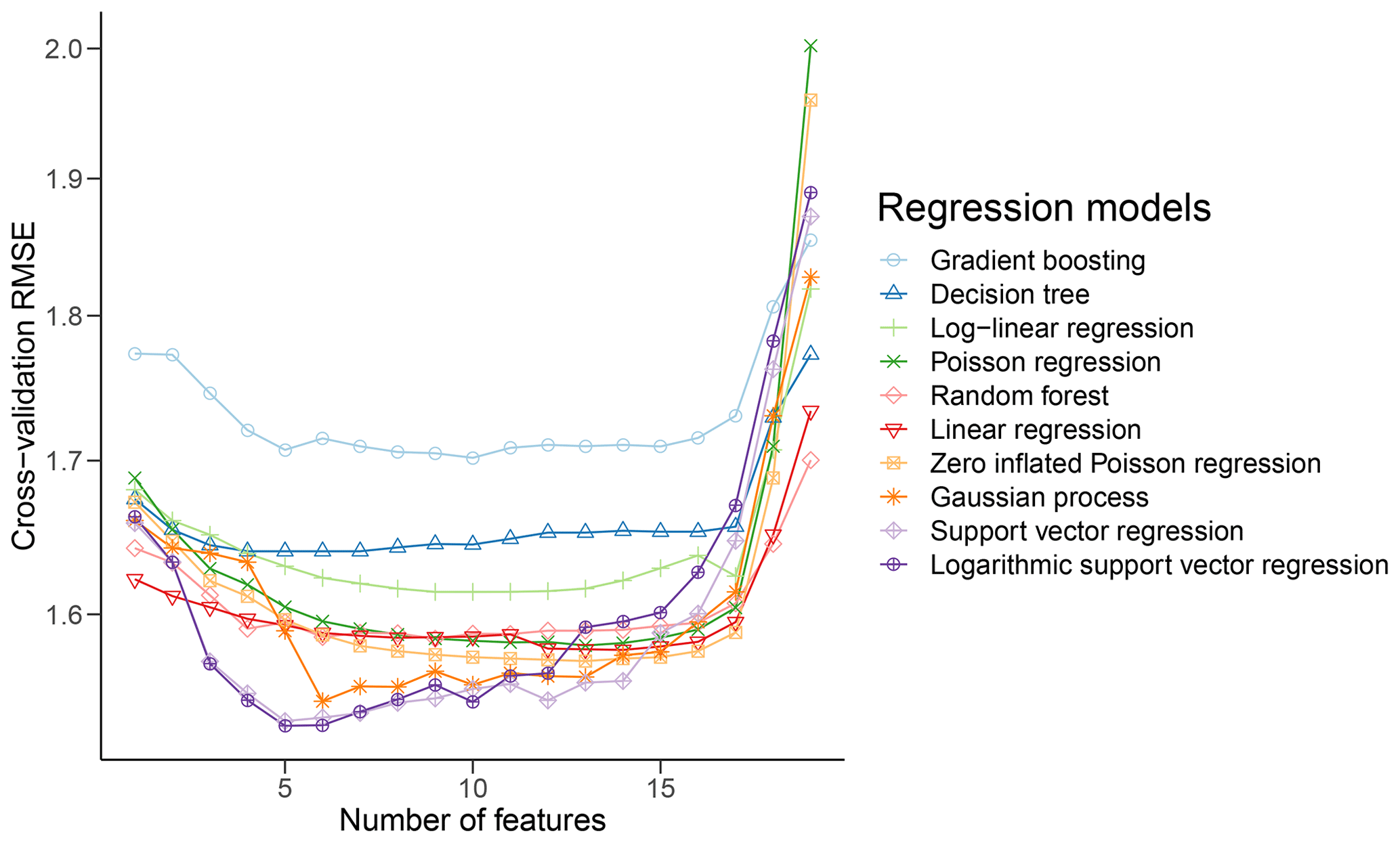
For each model, forward feature selection on KU18 provides the optimal set of features (as described in Sect. 2.3). Figure 4 shows the results of feature selection. Features are iteratively added (x axis) and cv-RMSE is computed (y axis). For each model, the features are selected such that cv-RMSE is minimized. In order to limit the computation time of feature selection, SVR and GPR were trained on a random subset of 2500 data points (out of the total 472 991), rather than the whole cross-validation split.
After feature selection, each model is trained on the whole training data (all KU18 city plans), using the optimal features from feature selection. SVR and GPR are, as in feature selection, only trained on 2500 randomly selected data points.
SVR and GPR have additional parameters whose optimal values were computed using grid search. Grid search is a model tuning technique in which the model is trained using all parameter values on a discrete grid of the parameter space. The selection criterion for the optimal parameter values was cv-RMSE (as with feature selection).
Note that some models allow for negative predictions (negative pollutant concentrations), which is physically impossible. A possible approach for avoiding negative predictions is either to use a transformation that allows only positive predictions (for example, log-linear regression instead of linear regression) or to clip model outputs to a minimum of zero after prediction. For the purposes of this study, however, negative predictions are retained, since their magnitude is relevant for error estimation.
3.2 Model selection
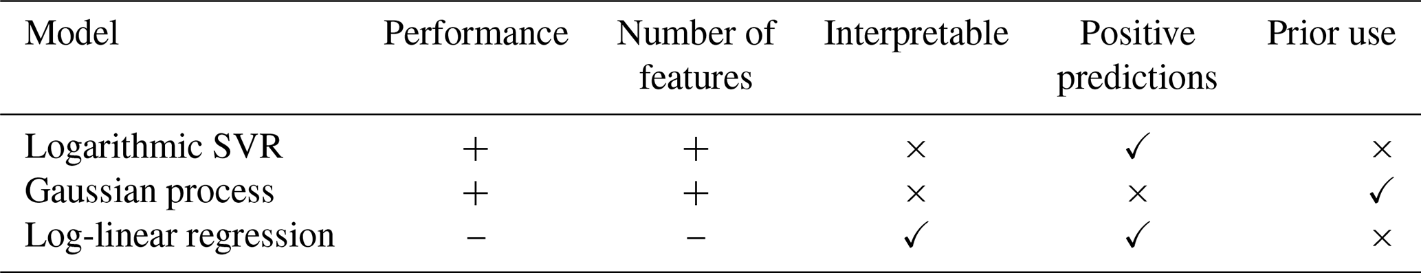
Out of the 10 models described in Sect. 2.4, three are selected as the best performing for replicating the LES outputs: logarithmic support vector regression, Gaussian process regression and log-linear regression. Table 3 compares the three selected models. Table 4 lists the performance of all 10 models with respect to cross-validation RMSE, mRMSE and scaled bias (described in Sect. 2.5). Performance evaluation at this stage is based on the cross-validation errors computed during forward feature selection on KU18. Final model evaluation on an independent dataset (KA20) is performed in Sect. 3.3.
The three best-performing models are as follows:
- Logarithmic SVR
-
The logarithmic SVR has the smallest cross-validation RMSE, and as such, its predictions are the most accurate on the training data. Additionally, it only requires a small number of features to achieve this strong performance. Requiring low-dimensional training data means that the user will need to provide fewer features with their data, minimizing the expense of data preparation. A third advantage is that the log transformation ensures non-negative predictions for pc. Although the standard SVR does not ensure non-negative predictions, it requires the same number of features and offers almost the same RMSE.
- Gaussian process regression
-
The RMSE of the GPR is close to that of the log-SVR, making it one of the strongest models as well. In addition, it has previously been used to predict simulator outputs (Gómez-Dans et al., 2016).
- Log-linear regression
-
As a linear model, the log-linear regression is useful if model interpretability is required (for more details on its interpretability, see Sect. 2.4). What separates the log-linear regression from the other linear models is that it uses the fewest number of features, while also ensuring positive predictions through log transformation, similar to the logarithmic SVR. It works as a simpler counterpart to the more powerful methods.
Table 3Comparison of selected models based on KU18. Performance refers to the cross-validated RMSE; number of features refers to the optimal number selected during forward feature selection. Prior use means the model has been used for similar tasks in literature. A “+” means better than average, which is not necessarily more than average.
3.3 Model evaluation
As a final test, the models are evaluated on an independent dataset to obtain a more accurate estimate of their performance in a real-world urban planning situation. The models cannot be evaluated solely based on the training data, since model overfitting would not be detected, and the error estimation in real-world situations would be poor. For the evaluation, we use the models trained on both wind directions and all city plans of KU18 (as described in Sect. 3.1) and we evaluate them on both wind directions of KA20.
We use the mRMSE and the scaled bias defined in Sect. 2.5 for KA20, with the results for PM2.5 concentrations listed in Table 4. Due to the scaling, the mRMSE does not allow direct comparisons between the errors on KU18 and KA20. On the evaluation data, we can however compare the models to the dummy model and see that, with the exception of the Poisson regressions, all models clearly outperform the dummy model, although the performance is more varied than with the training data. The best-performing model is the log-linear model (mRMSE = 0.76). The log-SVR and GPR also performed well (mRMSE = 0.87 and mRMSE = 0.91, respectively) when compared to the dummy model (mRMSE = 1.78).
Out of the selected models, the log-linear model is preferable. Not only does it perform the best out of all the three models selected but it is also the simplest and it runs the fastest. Its simplicity is likely the reason for its good performance given the notable differences between the training and evaluation data.
Although log-SVR and GPR both perform better than the average model, compared to the other models, their performance is worse in the evaluation data when comparing to the cross-validation procedure. This could be a sign of slight overfitting to the training data or sensitivity of the different distribution of data on the testing dataset.
The interpretation of the scaled bias is not straightforward due to the scaling, but it shows that all of the models overestimate pc in the evaluation data with the SVR overestimating the least. The dummy model is, unsurprisingly, the most biased.
The scaled residuals can be seen in Fig. 5 for the selected models. At a glance, they may seem to be similar for different models but there are differences between the predictions displayed even by the different mRMSE. The differences are due to the dissimilar ways of building a model and the features selected in Sect. 2.3. All three selected models acquire most of the error on the boulevard, while the outskirts are predicted more consistently. This is not a surprise since pc is much lower outside of the boulevard. The figure also show that the log-linear model has more balanced residuals while the more complex SVR and GPR are able to achieve lower residuals on the outskirts but perform relatively poorly on the boulevard. The residuals also show that none of the models are fully capable of capturing details in the pollutant dispersion that arise due to fine-scale flow patterns.
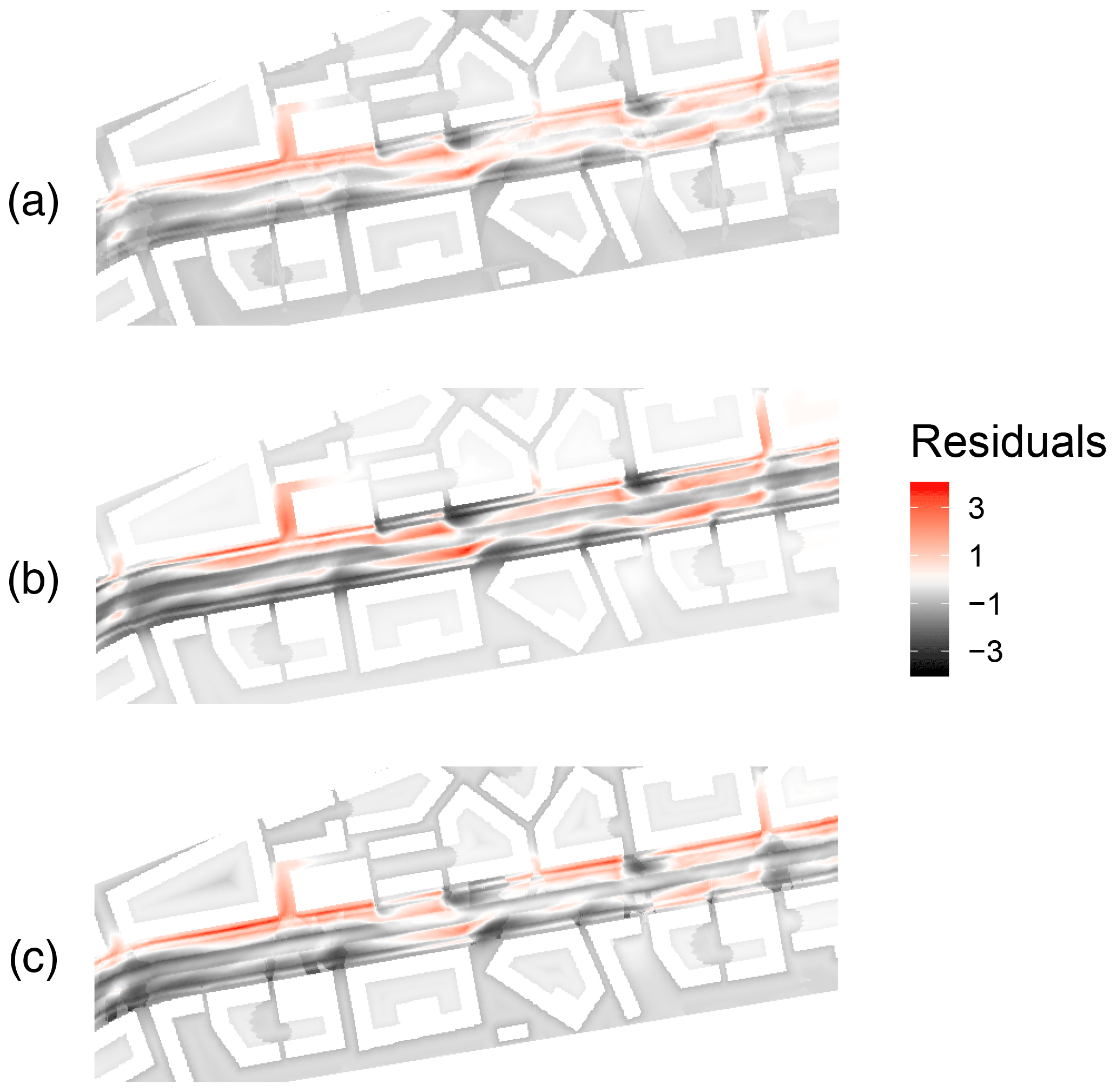
Figure 5Model residuals of PM2.5 predictions in KA20 for (a) the log-linear regression, (b) the logarithmic SVR and (c) the Gaussian process. The wind is coming from the left. Residuals are calculated after scaling with the respective optimal a for mRMSE calculation. Notice that although the residuals look similar, the predictions have notable differences. The scaled pc ranges up to a maximum of 7.28. The residuals can also be contrasted to the mean squared error of the dummy model, which is 1.78.
Table 4Cross validation and evaluation error for all models, obtained with their respective optimal set of features. Cross-validation RMSE is on KU18, while mRMSE and scaled bias are calculated on PM2.5 in KA20. In bold are the three models that were ultimately selected for performance (based on cross-validation RMSE) or interpretability.

3.4 Concept drift detection
It is important to know whether the results obtained generalize to different city plans. Because of the high computational cost of running LES, we often do not have access to the LES output values of a new plan, and hence we cannot assess the prediction error directly in such a case. We can, however, use the Drifter algorithm by Oikarinen et al. (2021) to estimate whether RMSE of a model prediction is high or not. The Drifter algorithm is designed for detecting “virtual concept drift”; (Gama et al., 2014), i.e. detecting changes in the distribution of the features that affect the performance of the model. The idea behind Drifter is that we define a distance measure d(x) that measures how far a covariate vector x is from the data that have been used to train the model. Small values of d(x), which is called the “concept drift indicator”, mean that we are close to the training data and the model should be reliable, while a large value of d(x) means that we have moved away from the training data, after which the regression estimate may be inaccurate. The distance measure d(x) is defined as follows. First, a family of so-called “segment models” fi is trained using only a part of the training data for each. Then, for each of the segment models fi, we can compute an estimate of the generalization error using the terms (f(x)−fi(x))2 instead of the terms (f(x)−pc)2, where pc is the LES output value, when computing the RMSE. For a simple linear model, this kind of a measure is monotonically related to the expected quadratic error of the model (Oikarinen et al., 2021). Now, the ensemble of estimates for the segment models allows to compute a statistic for estimating RMSE. In Oikarinen et al. (2021), the statistic (i.e. the concept drift indicator d(x)) was chosen to be the second smallest error estimate.

Figure 6Example of a single evaluation segment (light blue square) applied in the concept drift analysis for KA20 using the Drifter algorithm.
Originally, the Drifter algorithm has been used for time series data. We adapt it for spatial data here by selecting the segments of the training data not to be temporally close-by data points but spatially close-by points. We hence divide the map into k×k squares that are used as the segments. An example of such a segment can be seen in Fig. 6. Drifter is run for all models considered in Sect. 3.2 as the complete model. The original article suggests the usage of a simple linear model as the segment model, but here a ridge regression with logarithmic transformation and with a small regularization parameter of λ = 0.01 is chosen for practical reasons. This gives similar results to a log-linear model while also being well defined on the segments where some features are constant.

Figure 7The relationship between the concept drift indicator and observed RMSE in a given segment in KU18 (circles) and KA20 (crosses) with (a) log-linear regression, (b) logarithmic support vector regression, (c) Gaussian process and (d) log-linear regression with all features used as the complete model. The opacity of the training data has been reduced by 80 % to make the figure clearer.
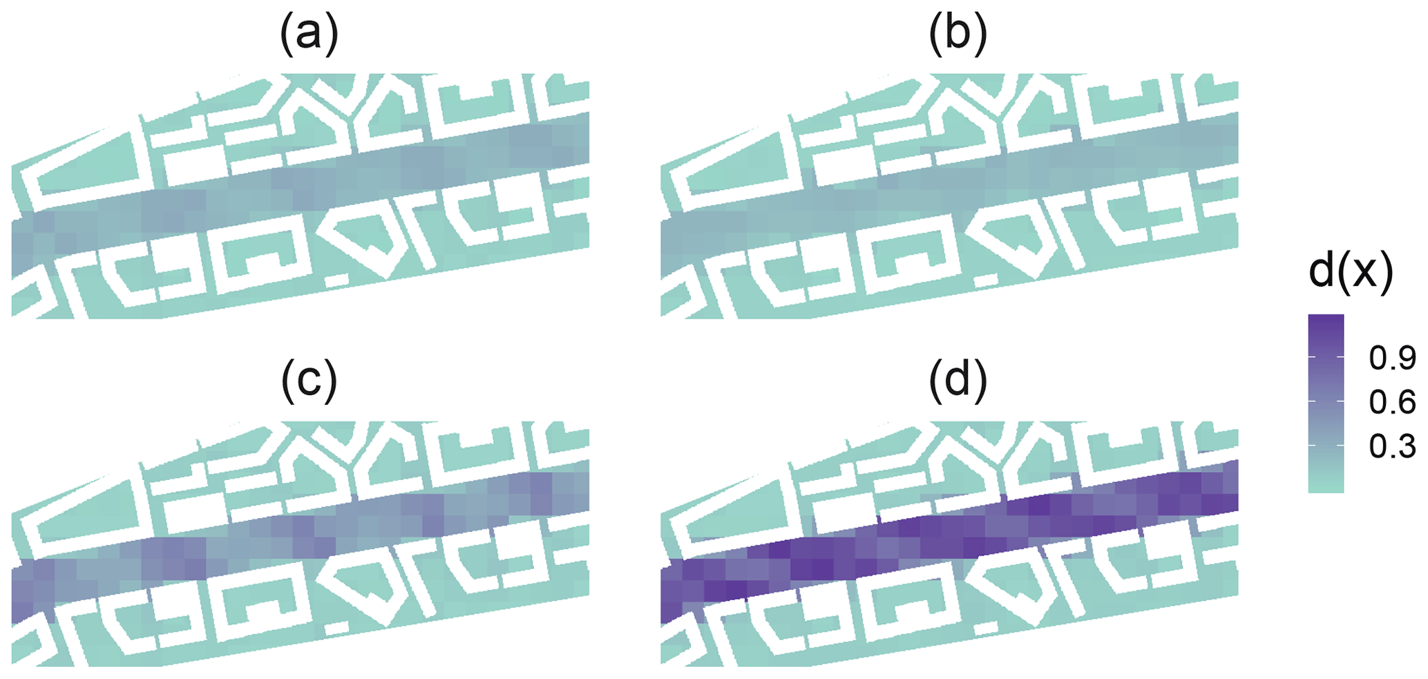
Figure 8A map showing the concept drift indicator d(x) in a given segment of KA20 for (a) log-linear regression, (b) logarithmic support vector regression, (c) Gaussian process and (d) log-linear regression with all features used as the complete model. Notice how the last model has a high concept drift indicator on the boulevard.
In order to keep the results comparable to Sect. 3, we also scale the evaluation dataset (KA20) by multiplying it with the constant that minimizes RMSE. This, if the evaluation data are not segmented, is equivalent to using the same multiplicative minimum-RMSE error measure as in Sect. 3. This decision does not affect the concept drift indicator but it will make the simulation error of the training and evaluation more comparable. We train Drifter using all eight simulation setups of KU18 (i.e. four city plans and two wind directions) and evaluate it on both wind directions of KA20. We use 100 m×100 m squares as our segments in the training data with each square overlapping 25 % out of four other training segments and 25 m×25 m squares in the evaluation data with no overlap. The concept drift indicator d(x) is chosen to be the tenth smallest error estimate. The overlapping scheme used is the same as in the original article, but since the data are two-dimensional, it is applied for both dimensions (50%⋅50 % = 25 %). These parameters are chosen with a grid search for the log-linear model with all features (a situation exhibiting concept drift).
In Fig. 7a–c, we show the concept drift indicator value and RMSE for each 25 m×25 m segment in the evaluation data alongside the same-sized segments in the training data for our final models in the same figure. With all three models considered, the evaluation data concept drift indicator is indeed correlated with its RMSE and thus can be used to estimate it. We also notice that for all three models the evaluation segments lie in the same area as the training segments indicating the lack of concept drift. In addition, we notice that the concept drift indicator values are larger on the boulevard which corresponds to the fact that the RMSE is indeed larger there. Therefore, the concept drift indicator is useful in detecting areas of large RMSE even when if the ground truth (LES output) are not known.
Another example of the concept drift detection is given by testing Drifter with a sub-optimally performing model. If the same procedure is done for the log-linear model with all of the surrogate features and not with the set selected by forward selection, the model overfits. Unlike in the models above, we see from Fig. 7d that multiple evaluation segments lie on the right of the cluster of the training segments indicating concept drift. These points also have a higher RMSE which shows that Drifter is working as intended. From Fig. 8d, we see that concept drift is detected only on the boulevard which is as expected, because also the RMSEs are higher there.
This study demonstrates that machine-learning methods trained with LES data can be used to model street-level pollutant concentrations in a city-boulevard-type urban neighbourhood. The accuracy of the models is explored with an independent evaluation dataset to ensure their applicability in urban planning for new, similar types of neighbourhoods.
The log-linear regression has the greatest potential for replicating LES results even with a relatively small amount of data. It also has much potential in helping to understand which urban features govern local pollutant concentrations. The kernelized methods, SVR and GPR, show moderate performance and perform generally well in capturing the local mean concentration. However, all three have trouble in representing smaller-scale details in the concentration fields linked to turbulence. Furthermore, all models perform worse on the boulevard than in its surroundings. Still, these models beat the dummy model by a notable margin (e.g. RMSE ≤0.91 for the selected models compared to RMSE = 1.78 for the dummy model). In general, bias in the models is slightly negative.
No previous studies on applying LES air pollution data to train a machine-learning model exist, and therefore direct comparison is unfeasible. Also comparing to studies applying spatial air quality measurements (Adams and Kanaroglou, 2016; Hu et al., 2017; Krecl et al., 2019; Van den Bossche et al., 2018) is difficult, as the spatial resolution of the training data is of the lower order of magnitude. Still, some linkage can be found. Adams and Kanaroglou (2016), Krecl et al. (2019) and Van den Bossche et al. (2018) used mobile air quality measurements to train their models to produce spatial air quality predictions and concluded that the models tend to underestimate the localized peak values, as also shown in this study. Peng et al. (2017) also found that linear models lead to a smaller bias for a short data record when applying modelled air quality data to conduct up to 48 h air quality predictions. On the contrary, SVR was shown to outperform all other methods in Hu et al. (2017). However, their data had a spatial resolution of 15 m or more, which can explain why the other models had trouble generalizing the data. To achieve the best generalization and to avoid overfitting, Van den Bossche et al. (2018) stresses the importance of high-quality model predictors, high temporal and spatial resolution of training data and evaluation against an independent dataset, which are all fulfilled in this study.
A downside of the developed models is that, when applied to a new city plan, they require the plan to lead to a similar statistical distribution of the pollutant concentrations as the ones used for training, which means that the models have to cope with moderate amounts of concept drift. We can, however, detect this to avoid potentially false predictions that may occur when applying the models on data that do not follow the training distribution. Yet another limitation is the small number of simulation setups of the data: there are only eight different simulation setups (i.e. four city plans and two wind directions) to train with, which rules out methods requiring large annotated training datasets, such as some applications of deep learning. With more data, the models could potentially reach completely another level of accuracy. Another way to improve the accuracy would be to have even better and more capturing features. If very accurate results are needed, running a new LES is still the best approach. Still, model predictions are accurate enough for many purposes, such as to study pollutant exposure and to support urban planning.
The developed methods can be used to further probe new meteorological conditions and city plans. In a future study, these models could help us to understand how simple changes into the layout of the city plan, e.g. a new building, affect the local air pollutant concentrations. Eventually similar models could also be used to understand the complicated phenomena in simple urban areas.
To conclude, we have explored using different machine-learning models how to emulate air pollutant concentrations as simulated using LES. We use LESs made over two different boulevard-type street canyons to study the impact of building-block layouts on air pollutant concentrations. We examine the performance of 10 machine-learning methods by using site-specific features to predict the surface-level concentrations over the neighbourhoods. A total of 20 features are determined from the LES inputs and outputs. The results show how the studied machine-learning methods are able to produce the mean pollutant concentrations. Further, concept drift detection is used to detect areas where the model cannot be trusted and more simulation runs may be needed.
Table A1Detailed descriptions of features in Table 1. The Supplement contains visualizations of these features. Note that these features were computed with the help of auxiliary features that are not listed here, such as is_building, is_inhabited and is_intersection. For more details, see the supplied software code.

The code to reproduce the regression models is available at https://doi.org/10.5281/zenodo.3999302 (Lange et al., 2021). The input and output data for KU18 are available at http://urn.fi/urn:nbn:fi:att:cfe1bd77-6697-44b5-bdd7-ee74f36c7dcd (Kurppa et al., 2021). The input data for KA20 are available at https://doi.org/10.5281/zenodo.3556287 (Karttunen and Kurppa, 2021a) and the output data are available at http://urn.fi/urn:nbn:fi:att:ee275362-3f56-477c-bbbc-6fcacd9c7f95 (Karttunen and Kurppa, 2021b).
The supplement related to this article is available online at: https://doi.org/10.5194/gmd-14-7411-2021-supplement.
LJ, MK, KP and EO designed the concept of the study. ML and HS pre-processed the LES outputs, prepared and conducted the machine-learning simulations and statistical analyses with contributions from EO, RS and KP. LJ and MK provided expert advice on the LES model inputs and outputs. All co-authors participated in writing the manuscript with contributions from all co-authors.
The authors declare that they have no conflict of interest.
Publisher’s note: Copernicus Publications remains neutral with regard to jurisdictional claims in published maps and institutional affiliations.
For financial support we would like to thank the Academy of Finland (profiling action 3 and decisions 326280 and 326339), Helsinki Institute for Information Technology HIIT, the Doctoral Programme in Atmospheric Sciences (ATM-DP), and the Doctoral Programme in Computer Science (DoCS) at the University of Helsinki, and SMart URBan Solutions for air quality, disasters and city growth (SMURBS, no. 689443) funded by ERA-NET-Cofund project under ERA-PLANET.
This research has been supported by the Academy of Finland (grant nos. 326280, 326339, 320182), the Helsinki Institute for Information Technology HIIT, the Doctoral Programme in Atmospheric Sciences (ATM-DP), University of Helsinki, the Doctoral Programme in Computer Sciences (DoCS), University of Helsinki, and the ERA-NET-Cofund, ERA-PLANET (grant no. 689443).
Open-access funding was provided by the Helsinki University Library.
This paper was edited by Adrian Sandu and reviewed by two anonymous referees.
Adams, M. D. and Kanaroglou, P. S.: Mapping real-time air pollution health risk for environmental management: Combining mobile and stationary air pollution monitoring with neural network models, J. Environ. Manag., 168, 133–141, https://doi.org/10.1016/j.jenvman.2015.12.012, 2016. a, b, c
Araki, S., Shima, M., and Yamamoto, K.: Spatiotemporal land use random forest model for estimating metropolitan NO2 exposure in Japan, Sci. Total Environ., 634, 1269–1277, https://doi.org/10.1016/j.scitotenv.2018.03.324, 2018. a
Auvinen, M., Boi, S., Hellsten, A., Tanhuanpää, T., and Järvi, L.: Study of realistic urban boundary layer turbulence with high-resolution large-eddy simulation, Atmosphere, 11, 201, https://doi.org/10.3390/atmos11020201, 2020. a
Benoit, K.: Linear regression models with logarithmic transformations, London School of Economics, London, 22, 23–36, 2011. a
Britter, R. E. and Hanna, S. R.: Flow and dispersion in urban areas, Ann. Rev. Fluid Mech., 35, 469–496, https://doi.org/10.1146/annurev.fluid.35.101101.161147, 2003. a
Cristianini, N. and Shawe-Taylor, J.: An Introduction to Support Vector Machines and Other Kernel-based Learning Methods, Cambridge University Press, Cambridge, United Kingdom, https://doi.org/10.1017/CBO9780511801389, 2000. a
Feng, R., Zheng, H.-J., Gao, H., Zhang, A.-R., Huang, C., Zhang, J.-X., Luo, K., and Fan, J.-R.: Recurrent Neural Network and random forest for analysis and accurate forecast of atmospheric pollutants: A case study in Hangzhou, China, J. Cleaner Product., 231, 1005–1015, https://doi.org/10.1016/j.jclepro.2019.05.319, 2019. a
Fernández-Delgado, M., Cernadas, E., Barro, S., and Amorim, D.: Do We Need Hundreds of Classifiers to Solve Real World Classification Problems?, J. Mach. Learn. Res., 15, 3133–3181, 2014. a
Gama, J. A., Žliobaitundefined, I., Bifet, A., Pechenizkiy, M., and Bouchachia, A.: A Survey on Concept Drift Adaptation, ACM Comput. Surv., 46, 44, https://doi.org/10.1145/2523813, 2014. a
Gómez-Dans, J. L., Lewis, P. E., and Disney, M.: Efficient Emulation of Radiative Transfer Codes Using Gaussian Processes and Application to Land Surface Parameter Inferences, Remote Sensing, 8, https://doi.org/10.3390/rs8020119, 2016. a
Hastie, T., Tibshirani, R., and Friedman, J.: The Elements of Statistical Learning, Springer-Verlag, 2009. a, b
Heus, T., van Heerwaarden, C. C., Jonker, H. J. J., Pier Siebesma, A., Axelsen, S., van den Dries, K., Geoffroy, O., Moene, A. F., Pino, D., de Roode, S. R., and Vilà-Guerau de Arellano, J.: Formulation of the Dutch Atmospheric Large-Eddy Simulation (DALES) and overview of its applications, Geosci. Model Dev., 3, 415–444, https://doi.org/10.5194/gmd-3-415-2010, 2010. a
Hu, K., Rahman, A., Bhrugubanda, H., and Sivaraman, V.: HazeEst: Machine Learning Based Metropolitan Air Pollution Estimation From Fixed and Mobile Sensors, IEEE Sensors J., 17, 3517–3525, https://doi.org/10.1109/JSEN.2017.2690975, 2017. a, b, c
Karttunen, S., Kurppa, M., Auvinen, M., Hellsten, A., and Järvi, L.: Large-eddy simulation of the optimal street-tree layout for pedestrian-level aerosol particle concentrations – A case study from a city-boulevard, Atmos. Environ., 6, 100073, https://doi.org/10.1016/j.aeaoa.2020.100073, 2020. a, b, c, d
Karttunen, S. and Kurppa, M.: Input data for article “Large eddy simulation of the optimal street-tree layout for pedestrian-level aerosol particle concentrations”, Zenodo [data set], https://doi.org/10.5281/zenodo.3556287, 2021a. a
Karttunen, S. and Kurppa, M.: Input and output files and datasets for a LES case study of city-boulevard ventilation, Fairdata [data set], available at: http://urn.fi/urn:nbn:fi:att:ee275362-3f56-477c-bbbc-6fcacd9c7f95, last access: 22 November 2021. a
King, R. N., Adcock, C., Annoni, J., and Dykes, K.: Data-Driven Machine Learning for Wind Plant Flow Modeling, J. Phys. Conf. Ser., 1037, 072004, https://doi.org/10.1088/1742-6596/1037/7/072004, 2018. a
Krecl, P., Cipoli, Y. A., Targino, A. C., de Oliveira Toloto, M., Segersson, D., Ãlvaro Parra, Polezer, G., Godoi, R. H. M., and Gidhagen, L.: Modelling urban cyclists' exposure to black carbon particles using high spatiotemporal data: A statistical approach, Sci. Total Environ., 679, 115–125, https://doi.org/10.1016/j.scitotenv.2019.05.043, 2019. a, b, c
Kumar, P., Ketzel, M., Vardoulakis, S., Pirjola, L., and Britter, R.: Dynamics and dispersion modelling of nanoparticles from road traffic in the urban atmospheric environment – A review, J. Aerosol Sci., 42, 580–603, https://doi.org/10.1016/j.jaerosci.2011.06.001, 2011. a
Kurppa, M., Hellsten, A., Auvinen, M., Raasch, S., Vesala, T., and Järvi, L.: Ventilation and Air Quality in City Blocks Using Large-Eddy Simulation—Urban Planning Perspective, Atmosphere, 9, 65, https://doi.org/10.3390/atmos9020065, 2018. a, b, c, d, e, f
Kurppa, M., Hellsten, A., Roldin, P., Kokkola, H., Tonttila, J., Auvinen, M., Kent, C., Kumar, P., Maronga, B., and Järvi, L.: Implementation of the sectional aerosol module SALSA2.0 into the PALM model system 6.0: model development and first evaluation, Geosci. Model Dev., 12, 1403–1422, https://doi.org/10.5194/gmd-12-1403-2019, 2019. a
Kurppa, M., Helssten, A., Auvinen, M., and Järvi, L.: Assessing pollutant ventilation in a city-boulevard using large-eddy simulation, Fairdata [data set], available at: http://urn.fi/urn:nbn:fi:att:cfe1bd77-6697-44b5-bdd7-ee74f36c7dcd, last access: 22 November 2021. a
Lambert, D.: Zero-Inflated Poisson Regression, With an Application to Defects in Manufacturing, Technometrics, 34, 1–14, 1992. a
Lange, M., Suominen, H., Kurppa, M., Järvi, L., Oikarinen, E., Savvides, R., and Puolamäki, K.: Datasets of Air Pollutants on Boulevard Type Streets and Software to Replicate Large-Eddy Simulations of Air Pollutant Concentrations Along Boulevard-Type Streets (1.0.0), Zenodo [data set and code], https://doi.org/10.5281/zenodo.3999302, 2021. a
Lelieveld, J., Evans, J. S., Fnais, M., Giannadaki, D., and Pozzer, A.: The contribution of outdoor air pollution sources to premature mortality on a global scale, Nature, 525, 367–371, https://doi.org/10.1038/nature15371, 2015. a
Lelieveld, J., Klingmüller, K., Pozzer, A., Pöschl, U., Fnais, M., Daiber, A., and Münzel, T.: Cardiovascular disease burden from ambient air pollution in Europe reassessed using novel hazard ratio functions, Eur. Heart J., 40, 1590–1596, https://doi.org/10.1093/eurheartj/ehz135, 2019. a
Maronga, B., Gryschka, M., Heinze, R., Hoffmann, F., Kanani-Sühring, F., Keck, M., Ketelsen, K., Letzel, M. O., Sühring, M., and Raasch, S.: The Parallelized Large-Eddy Simulation Model (PALM) version 4.0 for atmospheric and oceanic flows: model formulation, recent developments, and future perspectives, Geosci. Model Dev., 8, 2515–2551, https://doi.org/10.5194/gmd-8-2515-2015, 2015. a
Maronga, B., Banzhaf, S., Burmeister, C., Esch, T., Forkel, R., Fröhlich, D., Fuka, V., Gehrke, K. F., Geletič, J., Giersch, S., Gronemeier, T., Groß, G., Heldens, W., Hellsten, A., Hoffmann, F., Inagaki, A., Kadasch, E., Kanani-Sühring, F., Ketelsen, K., Khan, B. A., Knigge, C., Knoop, H., Krč, P., Kurppa, M., Maamari, H., Matzarakis, A., Mauder, M., Pallasch, M., Pavlik, D., Pfafferott, J., Resler, J., Rissmann, S., Russo, E., Salim, M., Schrempf, M., Schwenkel, J., Seckmeyer, G., Schubert, S., Sühring, M., von Tils, R., Vollmer, L., Ward, S., Witha, B., Wurps, H., Zeidler, J., and Raasch, S.: Overview of the PALM model system 6.0, Geosci. Model Dev., 13, 1335–1372, https://doi.org/10.5194/gmd-13-1335-2020, 2020. a
Murphy, K. P.: Machine Learning: A Probabilistic Perspective, The MIT Press, Cambridge, Massachusetts, 2012. a, b
Nosek, Š., Kukačka, L., Kellnerová, R., Jurčáková, K., and Jaňour, Z.: Ventilation Processes in a Three-Dimensional Street Canyon, Bound.-Lay. Meteorol., 159, 259–284, https://doi.org/10.1007/s10546-016-0132-2, 2016. a
Oikarinen, E., Tiittanen, H., Henelius, A., and Puolamäki, K.: Detecting virtual concept drift of regressors without ground truth values, Data Min. Knowl. Disc., 35, 726–747, https://doi.org/10.1007/s10618-021-00739-7, 2021. a, b, c
Peng, H., Lima, A. R., Teakles, A., Jin, J., Cannon, A. J., and Hsieh, W. W.: Evaluating hourly air quality forecasting in Canada with nonlinear updatable machine learning methods, Air Quality, Atmos. Health, 10, 195–211, https://doi.org/10.1007/s11869-016-0414-3, 2017. a, b
R Core Team: R: A Language and Environment for Statistical Computing, R Foundation for Statistical Computing, Vienna, Austria, avilable at: https://www.R-project.org/ (last access: 22 November 2021), 2020. a
Rybarczyk, Y. and Zalakeviciute, R.: Machine Learning Approaches for Outdoor Air Quality Modelling: A Systematic Review, Appl. Sci., 8, 2570, https://doi.org/10.3390/app8122570, 2018. a, b
Salim, S. M., Buccolieri, R., Chan, A., and Sabatino, S. D.: Numerical simulation of atmospheric pollutant dispersion in an urban street canyon: Comparison between RANS and LES, J. Wind Eng. Ind. Aerod., 99, 103–113, https://doi.org/10.1016/j.jweia.2010.12.002, 2011. a
Tominaga, Y. and Stathopoulos, T.: CFD modeling of pollution dispersion in a street canyon: Comparison between LES and RANS, J. Wind Eng. Ind. Aerod., 99, 340–348, https://doi.org/10.1016/j.jweia.2010.12.005, 2011. a
Van den Bossche, J., Baets, B. D., Verwaeren, J., Botteldooren, D., and Theunis, J.: Development and evaluation of land use regression models for black carbon based on bicycle and pedestrian measurements in the urban environment, Environ. Model. Softw., 99, 58–69, https://doi.org/10.1016/j.envsoft.2017.09.019, 2018. a, b, c, d
WHO (World Health Organization): Ambient air pollution: A global assessment of exposure and burden of disease, available at: https://apps.who.int/iris/handle/10665/250141 (last access: 22 November 2021), 2016. a
Yang, W., Deng, M., Xu, F., and Wang, H.: Prediction of hourly PM2.5 using a space-time support vector regression model, Atmos. Environ., 181, 12–19, https://doi.org/10.1016/j.atmosenv.2018.03.015, 2018. a
Yuan, C., Ng, E., and Norford, L. K.: Improving air quality in high-density cities by understanding the relationship between air pollutant dispersion and urban morphologies, Build. Environ., 71, 245–258, https://doi.org/10.1016/j.buildenv.2013.10.008, 2014. a
- Abstract
- Introduction
- Methods and material
- Experiments
- Discussion and conclusions
- Appendix A: Detailed descriptions of the features used in the regression models
- Code and data availability
- Author contributions
- Competing interests
- Disclaimer
- Acknowledgements
- Financial support
- Review statement
- References
- Supplement