Evaluation of global EMEP MSC-W (rv4.34) WRF (v3.9.1.1) model surface concentrations and wet deposition of reactive N and S with measurements

Atmospheric pollution has many profound effects on human health, ecosystems, and the climate. Of concern are high concentrations and deposition of reactive nitrogen (N_r) species, especially of reduced N (gaseous NH₃, particulate ${{\mathrm{NH}}_{\mathrm{4}}}^{+}$). Atmospheric chemistry and transport models (ACTMs) are crucial to understanding sources and impacts of N_r chemistry and its potential mitigation. Here we undertake the first evaluation of the global version of the EMEP MSC-W ACTM driven by WRF meteorology ($\mathrm{1}{}^{\circ }\times \mathrm{1}{}^{\circ }$ resolution), with a focus on surface concentrations and wet deposition of N and S species relevant to investigation of atmospheric N_r and secondary inorganic aerosol (SIA). The model–measurement comparison is conducted both spatially and temporally, covering 10 monitoring networks worldwide. Model simulations for 2010 compared use of both HTAP and ECLIPSE_E (ECLIPSE annual total with EDGAR monthly profile) emissions inventories; those for 2015 used ECLIPSE_E only. Simulations of primary pollutants are somewhat sensitive to the choice of inventory in places where regional differences in primary emissions between the two inventories are apparent (e.g. China) but are much less sensitive for secondary components. For example, the difference in modelled global annual mean surface NH₃ concentration using the two 2010 inventories is 18 % (HTAP: 0.26 µg m⁻³; ECLIPSE_E: 0.31 µg m⁻³) but is only 3.5 % for ${{\mathrm{NH}}_{\mathrm{4}}}^{+}$ (HTAP: 0.316 µg m⁻³; ECLIPSE_E: 0.305 µg m⁻³). Comparisons of 2010 and 2015 surface concentrations between the model and measurements demonstrate that the model captures the overall spatial and seasonal variations well for the major inorganic pollutants NH₃, NO₂, SO₂, HNO₃, ${{\mathrm{NH}}_{\mathrm{4}}}^{+}$, ${{\mathrm{NO}}_{\mathrm{3}}}^{-}$, and ${{\mathrm{SO}}_{\mathrm{4}}}^{\mathrm{2}-}$ and their wet deposition in East Asia, Southeast Asia, Europe, and North America. The model shows better correlations with annual average measurements for networks in Southeast Asia (mean R for seven species: $\stackrel{\mathrm{‾}}{R_{\mathrm{7}}}=\mathrm{0.73}$), Europe ($\stackrel{\mathrm{‾}}{R_{\mathrm{7}}}=\mathrm{0.67}$), and North America ($\stackrel{\mathrm{‾}}{R_{\mathrm{7}}}=\mathrm{0.63}$) than in East Asia ($\stackrel{\mathrm{‾}}{R_{\mathrm{5}}}=\mathrm{0.35}$) (data for 2015), which suggests potential issues with the measurements in the latter network. Temporally, both model and measurements agree on higher NH₃ concentrations in spring and summer and lower concentrations in winter. The model slightly underestimates annual total precipitation measurements (by 13 %–45 %) but agrees well with the spatial variations in precipitation in all four world regions (0.65–0.94 R range). High correlations between measured and modelled ${{\mathrm{NH}}_{\mathrm{4}}}^{+}$ precipitation concentrations are also observed in all regions except East Asia. For annual total wet deposition of reduced N, the greatest consistency is in North America (0.75–0.82 R range), followed by Southeast Asia (R=0.68) and Europe (R=0.61). Model–measurement bias varies between species in different networks; for example, bias for ${{\mathrm{NH}}_{\mathrm{4}}}^{+}$ and ${{\mathrm{NO}}_{\mathrm{3}}}^{-}$ is largest in Europe and North America and smallest in East Asia and Southeast Asia. The greater uniformity in spatial correlations than in biases suggests that the major driver of model–measurement discrepancies (aside from differing spatial representativeness and uncertainties and biases in measurements) are shortcomings in absolute emissions rather than in modelling the atmospheric processes. The comprehensive evaluations presented in this study support the application of this model framework for global analysis of current and potential future budgets and deposition of N_r and SIA.

1 Introduction

In view of increasing growth in global anthropogenic emissions, the physical and chemical behaviour of reactive nitrogen (N_r) species, especially those that contain reduced N (i.e. gaseous NH₃ and particulate ${{\mathrm{NH}}_{\mathrm{4}}}^{+}$) have been explored in both experimental and modelling studies (Liu et al., 2019; Wagner et al., 2020; Ciarelli et al., 2019; Tang et al., 2021). As the predominant alkaline gas, NH₃ exerts significant control on the formation of ambient particles and the acidity of deposition. It readily reacts with H₂SO₄ and HNO₃ (respectively derived from emissions of SO₂ and NO_x), and the ammonium sulfate ((NH₄)₂SO₄) and nitrate (NH₄NO₃) particles formed in these reactions are important in Earth's radiation budget (Laskin et al., 2015) due to their capacity to act as cloud condensation nuclei and to absorb/scatter solar radiation. Crucially, the (NH₄)₂SO₄ and NH₄NO₃ secondary inorganic aerosols (SIAs) typically constitute at least a third of the fine particulate matter (PM_2.5) surface concentration (Li et al., 2017), exposure to which causes substantial premature mortality globally (Burnett et al., 2018). For half the world's population, the PM_2.5 air pollution burden is increasing (Shaddick et al., 2020). In addition, NH₃ and ${{\mathrm{NH}}_{\mathrm{4}}}^{+}$ enter aquatic and terrestrial ecosystems through wet and dry deposition, where they are powerful nutrients for many plants and microorganisms. As a result, excessive anthropogenic reduced N emissions to the atmosphere can lead to severe eutrophication and formation of hypoxic zones, with their consequent threats to ecosystem diversity (Erisman et al., 2005).

The surface concentrations and deposition fluxes of atmospheric pollutants are influenced by many spatial and temporal factors such as emissions, meteorology, long-distance transport, and chemical transformations. Ambient measurements play a vital role in assessing existing concentrations but can generally only represent the air quality in the local area and cannot immediately distinguish between the influence of local and remote sources. Speciated gas- and particle-phase sampling and analysis is challenging and expensive (Tang et al., 2018b). Consequently, measurements are generally sparsely located and often not very well temporally resolved, even in regions of the world with well-developed air pollution monitoring networks (Tang et al., 2021), which again limits the interpretation of atmospheric chemical and meteorological processes. Moreover, different world regions have monitoring networks that are subject to different analytical and data handling protocols, potentially leading to systematic differences. Non-identical sampling duration and frequencies within these networks also add uncertainties and complexities to global comparison studies.

Compared with measurements, global- and regional-scale atmospheric chemistry transport models such as EMEP MSC-W (Simpson et al., 2012), CMAQ (Byun and Schere, 2006), and WRF-Chem (Chapman et al., 2009) can provide comprehensive simulations of air pollutant concentrations and depositions with greater spatial and temporal resolution and coverage. These models also facilitate insight into the chemical and meteorological linkages between diverse emission sources and the concentration and deposition of pollutants at locations away from initial emissions. Such models are essential when it comes to simulating the impacts of possible future policy actions. A number of global models have already been utilized to investigate sulfate, nitrate, or ammonia budgets, including GISS II-prime (Adams et al., 1999), GEOS-Chem (Pye et al., 2009), LMDz-INCA (Hauglustaine et al., 2014), STOCHEM-CRI (Khan et al., 2020), and multi-model ensemble analysis (Tan et al., 2018). Bian et al. (2017) presented a budget analysis of global nitrate simulations from nine models and found wide variation in the tropospheric burdens of HNO₃, ${{\mathrm{NO}}_{\mathrm{3}}}^{-}$, NH₃, and ${{\mathrm{NH}}_{\mathrm{4}}}^{+}$ between the models. However, global simulations and evaluation of N_r species in atmospheric chemistry transport models remain rare. In particular, there has been little comparison between modelled surface concentrations and wet deposition of N_r species, especially NH₃ and ${{\mathrm{NH}}_{\mathrm{4}}}^{+}$, with regional ground-based measurement networks worldwide, which is the motivation for this work.

Here, we present for the first time a detailed evaluation of the global simulation performance of the EMEP MSC-W chemical transport model coupled with the WRF numerical weather model. Our aim was to compare model output temporally and spatially with available ambient measurements from nine monitoring networks in four global regions. A further aim was to examine the sensitivities of the model–measurement comparison to two different global emission inventories (HTAP v2 and ECLIPSE). The primary focus of the comparisons was on atmospheric concentrations and wet depositions of the N_r and SIA species. We also undertook evaluations for two meteorological years: 2010 and 2015.

2 Methods

2.1 Model description and set-up

The EMEP MSC-W atmospheric chemistry transport model has been developed by the European Monitoring and Evaluation Programme Meteorological Synthesizing Centre – West. As described by Simpson et al. (2012) and at https://www.emep.int (last access: 20 May 2021), EMEP MSC-W is an open-source Eulerian grid model used for applications ranging from scientific research to policy development (Bergström et al., 2014; Mills et al., 2018; Karl et al., 2019; Ciarelli et al., 2019; Jonson et al., 2017; McFiggans et al., 2019). The model uses 21 terrain-following vertical layers, with the pressure ranging from around 1000 hPa (surface level) to 100 hPa (highest level). We use a lowest layer of ∼45 m height. Output surface concentrations for major species are adjusted to be equivalent to 3 m above the surface as described in Simpson et al. (2012).

In this study, we utilize the most recent EMEP MSC-W model version rv4.34. Simpson et al. (2020) provide an overview of the changes made to the model since the version rv4.0 documented in Simpson et al. (2012). These changes include improved calculations of aerosol surface area and gas aerosol uptake (Stadtler et al., 2018); additional land cover classes and improved leaf area calculations for global biogenic volatile organic compound (BVOC) emission calculation (Simpson, 2017); a new radiation scheme (Weiss and Norman, 1985) for BVOC and deposition calculations; new chemical mechanisms (Bergström, 2021); and changes related to sea salt, dust, and other emissions handling.

Most studies using EMEP MSC-W utilize meteorological data from the Integrated Forecast System model (IFS) of the European Centre for Medium-Range Weather Forecasts (ECMWF) (Fagerli et al., 2019; Pommier et al., 2020; Simpson et al., 2012). Evaluations of the MSC-W model run with IFS meteorology can be found in Mills et al. (2018), who found good agreement of modelled versus measured O₃ metrics across the Global Atmosphere Watch network; McFiggans et al. (2019), who found good to reasonable agreement of organic aerosol data for European and North American networks; and Bian et al. (2017), who found reasonable agreement for inorganic S and N compounds in a multi-model study.

In contrast, the meteorology used for the EMEP MSC-W model simulations in this study was derived from the Weather Research and Forecast model (WRF, http://www.wrf-model.org, last access: 20 May 2021) version 3.9.1.1 (Skamarock, 2008) at grid resolution of $\mathrm{1}{}^{\circ }\times \mathrm{1}{}^{\circ }$. The WRF model included data assimilation (Newtonian nudging) of the numerical weather prediction model meteorological reanalysis from the US National Center for Environmental Prediction (NCEP)/National Center for Atmospheric Research (NCAR) Global Forecast System (GFS) at 1^∘ resolution every 6 h (Saha et al., 2010). This work uses the Yonsei University (YSU) planetary boundary layer (PBL) scheme. The bulk microphysical parameterization (BMP) scheme is from Lin et at. (2011). The cumulus parameterization uses the Kain–Fritsch scheme. The longwave and shortwave radiation scheme utilizes RRTM/Dudhia. The WRF simulations used the Noah Land Surface Model, for land cover set-up WRF uses the MODIS-derived land cover, and the EMEP MSC-W model uses land data from GLC2000 with the Community Land Model (CLM). The EMEP MSC-W model calculates roughness length and depositions from its own land cover. A higher-resolution UK and Europe regional version of the EMEP-WRF modelling system has previously been evaluated well against field measurements (Vieno et al., 2010, 2014, 2016). However, an assessment of the global version has not yet been undertaken. Moreover, integrating WRF with the EMEP MSC-W model is still an innovative application, as most studies utilize meteorological data from the IFS model as described above.

Two global emission inventories were used in this work. The ECLIPSE (Evaluating the CLimate and Air Quality ImPacts of Short-livEd Pollutant) inventory version V6 (https://iiasa.ac.at/web/home/research/researchPrograms/air/ECLIPSEv6b.html, last access: 20 May 2021) contains annual gridded emissions of SO₂, NO₂, NH₃, CO, CH₄, NMVOCs (non-methane volatile organic compounds), primary fine particulate matter (PM_2.5), and primary coarse particulate matter (PM_co) (Klimont et al., 2017) at $\mathrm{0.5}{}^{\circ }\times \mathrm{0.5}{}^{\circ }$ spatial resolution. Its emission sectors include energy, industry, solvent use, transport, domestic combustion, agriculture, open burning of agricultural waste, and waste treatment. We used ECLIPSE emission inventories for 2010 and 2015 to permit comparison between model and measurements for two self-consistent years of emissions, meteorology, and measurements. The HTAP (Task Force on Hemispheric Transport of Air Pollution) inventory version V2 (https://edgar.jrc.ec.europa.eu/dataset_htap_v2, last access: 20 May 2021) consists of $\mathrm{0.1}{}^{\circ }\times \mathrm{0.1}{}^{\circ }$ gridded monthly emissions of SO₂, NO₂, NH₃, CO, CH₄, NMVOCs, PM_2.5, PM₁₀, black carbon (BC), and organic carbon (OC) for 2010 (2015 was not available at the time of this work) from seven sectors (international and domestic air, shipping, energy, industry, transport, residential, and agriculture) and was used to investigate the sensitivity of model outputs to different global inventories. The HTAP inventory utilizes nationally reported emissions together with regional scientific inventories (e.g. from the U.S. EPA, the MICS-Asia group, EMEP/TNO, the REAS, and the EDGAR group) for those regions where national emissions are not available (Janssens-Maenhout et al., 2015; Gusev et al., 2012; West et al., 2010).

Both inventories were aggregated to $\mathrm{1}{}^{\circ }\times \mathrm{1}{}^{\circ }$ resolution internally in the model. All inventory emission sector layers were re-assigned to 11 selected nomenclature for sources of air pollution (SNAP) sectors: (1) combustion in energy and transformation industries, (2) non-industrial combustion plants, (3) combustion in manufacturing industry, (4) production processes, (5) extraction and distribution of fossil fuels and geothermal energy, (6) solvent and other product use, (7) road transport, (8) other mobile sources and machinery, (9) waste treatment and disposal, (10) agriculture, and (11) other sources and sinks.

In addition, monthly emission time series by sector and country derived from EDGAR (Emission Database for Global Atmospheric Research, v4.3.2 datasets) temporal emission profiles (Crippa et al., 2020) (https://edgar.jrc.ec.europa.eu/dataset_temp_profile, last access: 20 May 2021) were applied to the ECLIPSE annual total emissions for all pollutants. Therefore, from here on we refer to the inventory with ECLIPSE annual emissions and EDGAR monthly temporal profiles as ECLIPSE_E. All EDGAR emission subsectors (∼33) are further divided into 11 SNAP sectors. The time-splitting factor (T_SNAP) for a given pollutant for a given country or region was computed as follows. Annual average emission of pollutant from EDGAR v4.3.2 subsector j, ${\stackrel{\mathrm{‾}}{P}}_j$, was calculated as follows:

$${\stackrel{\mathrm{‾}}{P}}_j={\displaystyle \frac{{\sum }_{i=\mathrm{1}}^{\mathrm{12}}{P}_{ij}}{\mathrm{12}}}.$$

Monthly time-splitting factor of pollutant from subsector j, T_{E_j}, was calculated as follows:

$$T_{E\mathit{\_}j}={\displaystyle \frac{P_{ij}}{{\stackrel{\mathrm{‾}}{P}}_j}}.$$

The weight of T_{E_j} in month i was calculated as follows:

$$W_{ij}={\displaystyle \frac{P_{ij}}{{\sum }_{j=\mathrm{1}}^n{P}_{ij}}}.$$

The time-splitting factor for the EMEP MSC-W model SNAP sector in month i was calculated as follows:

$$T_{\text{SNAP}}={\displaystyle \frac{{\sum }_{j=\mathrm{1}}^n{T}_{E\mathit{\_}j}\times W_{ij}}{{\sum }_{j=\mathrm{1}}^n{W}_{ij}}}.$$

The EMEP MSC-W model default hour-of-day temporal profiles (which varies with SNAP sector) were applied to all countries. The default day-of-week temporal profile was applied to Europe only as neither of the emission inventories supply such temporal information.

Forest and vegetation fire emissions and international shipping emissions are also included in both inventories. Emissions of dimethyl sulfide (DMS), lightning NO_x, soil NO_x and isoprene are set as reported in Simpson et al. (2017, 2020), as are the wind-derived emissions of dust and sea salt (Simpson et al., 2012; Tsyro et al., 2011).

2.2 Measurement datasets

Ambient measurement data were compiled from the 10 regional and national monitoring networks in East Asia, Southeast Asia, Europe, and North America listed in Table 1. The number of monitoring sites in each network varies with year and with species, but Fig. 1 shows the monitoring sites for ${{\mathrm{NH}}_{\mathrm{4}}}^{+}$ in 2015 as an example. The frequency and duration (i.e. averaging) of sampling, and the sampling and analytical methods used, including the size fraction of PM sampled, vary across the measurement networks. Some measurement locations are also deliberately sited to be close to particular industrial or agricultural sources, in which case a model grid average concentration may not reflect the measurement. Although much of this information is presented in official network reports, much useful metadata is absent from the data portals and addition of this information directly to the portals is a recommendation for improvement. In this work, only measurement data with at least 75 % data capture in the year are used to avoid bias. A full data mining of global measurement data was not undertaken here, but we believe we have captured the major networks of long-running, multi-species SIA gas and particle composition and wet deposition measurements.

Table 1 Summary of surface monitoring networks used in the model–measurement comparisons. The last access date for all URLs cited in this table is 20 May 2021.

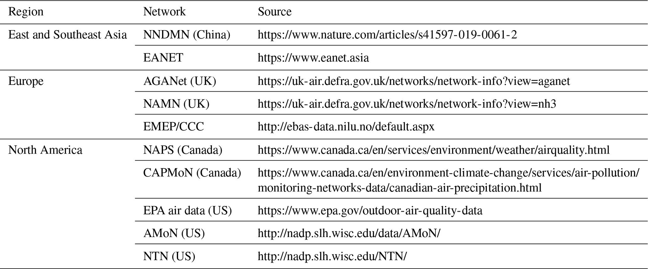
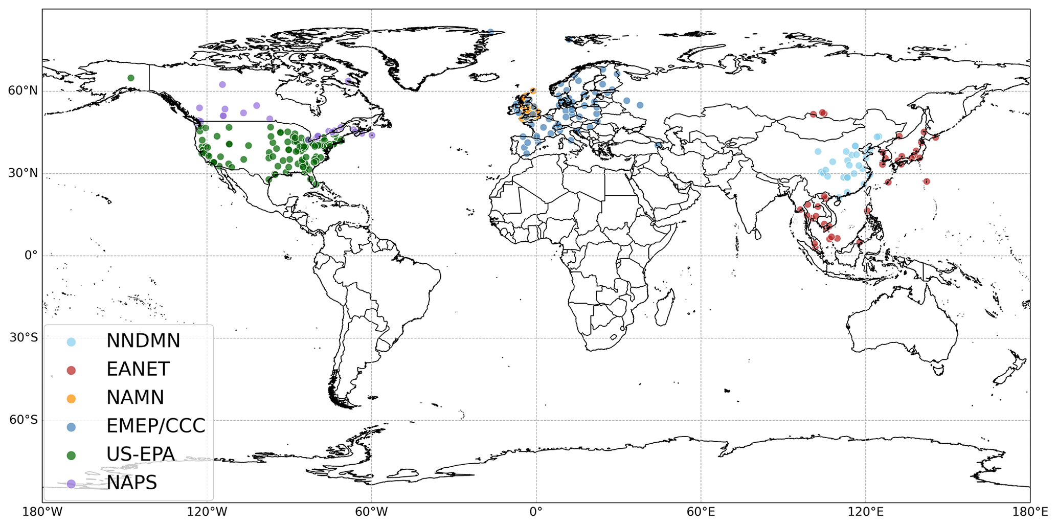
Figure 1 Locations of sites in the six networks that measured particle-phase ${{\mathrm{NH}}_{\mathrm{4}}}^{+}$ in 2015.

The Chinese national nitrogen deposition monitoring network (NNDMN) was established in 2010 to measure inorganic N concentrations and deposition fluxes. The first database, NNDMN 1.0, which compiles monthly air concentration and deposition data for NH₃, NO₂, HNO₃, ${{\mathrm{NH}}_{\mathrm{4}}}^{+}$, and ${{\mathrm{NO}}_{\mathrm{3}}}^{-}$ up to 2015 was released in May 2019 (Xu et al., 2019).

The acid deposition monitoring network in East Asia and Southeast Asia (EANET) involves 13 countries and provides annual and monthly concentration and acid deposition data for more than 10 species.

The UK Acid Gases and Aerosol Monitoring Network (AGANet, 30 sites) provides long-term national and monthly speciated measurements of acid gases (HNO₃, SO₂, HCl) and aerosol components (${{\mathrm{NO}}_{\mathrm{3}}}^{-}$, ${{\mathrm{SO}}_{\mathrm{4}}}^{\mathrm{2}-}$, Cl⁻, Na⁺, Ca²⁺, Mg²⁺) (Tang et al., 2018b). The UK National Ammonia Monitoring Network (NAMN, 95 sites) includes both AGANet and additional sites with monthly measurements of NH₃ and ${{\mathrm{NH}}_{\mathrm{4}}}^{+}$ (Tang et al., 2018a). Both NAMN and AGANet provide monthly average concentrations.

The European Monitoring and Evaluation Programme/Chemical Coordinating Centre (EMEP/CCC) is a collaborative programme for measuring air pollutants across Europe (Tørseth et al., 2012). The measurement frequency varies from hourly and daily to weekly and biweekly or intermittently, such as every 6 d. It also varies between species. This makes it difficult to derive consistent annual and monthly averages comparisons between measurement and model.

The air data of the United States Environmental Protection Agency (EPA) provides access to annual outdoor air quality data including SO₂, NO₂, ${{\mathrm{NH}}_{\mathrm{4}}}^{+}$, ${{\mathrm{NO}}_{\mathrm{3}}}^{-}$, and ${{\mathrm{SO}}_{\mathrm{4}}}^{\mathrm{2}-}$, collected from state, local, and tribal monitoring agencies across the United States. The Ammonia Monitoring Network (AMoN) and National Trends Network (NTN) are two further US networks, which provide long-term records of weekly or biweekly NH₃ gas concentrations and annual precipitation chemistries, respectively.

In Canada, the National Air Pollution Surveillance (NAPS) program is the main source of ambient air quality data and consists of continuous and time-integrated monitoring of several species. Continuous measurements are implemented for CO, NO₂, NO, NO_x, O₃, SO₂, PM_2.5, and PM₁₀ at hourly resolution. The time-integrated samples collect once per 6 d for a 24 h period, encompass fine (PM_2.5) and coarse (PM_2.5–10) aerosol components (e.g. inorganic ions, metals), semi-volatile organic compounds, and volatile organic compounds (VOCs). The Canadian Air and Precipitation Monitoring Network (CAPMoN) is designed to study the regional patterns and trends of atmospheric pollutants, such as acid rain, smog, particulate matter, and mercury, in both air and precipitation. Regional precipitation and wet deposition data from CAPMoN were collected through wet precipitation collectors.

The calculations of model–measurement comparison statistics (e.g. Pearson's correlation coefficient, mean bias, mean absolute error) are shown in the Supplement.

3 Results

3.1 Comparison between use of HTAP and ECLIPSE_E emission inventories

3.1.1 Emissions

The global map of 2010 annual NH₃ emissions from ECLIPSE_E is shown in Fig. 2a. Hot spots of NH₃ emissions occur across the globe in areas characterized by dense populations and intensive agricultural activities, most notably in the Indo-Gangetic Plain in India and the North China Plain but also Indonesia, Europe, United States, Mexico, and Brazil. The area-weighted average NH₃ emissions (over the whole global domain) in 2010 are 105 and 121 mg m⁻² for HTAP and ECLIPSE_E, respectively. The individual grid annual NH₃ emission in 2010 varies from 0.00 to 10 692 mg m⁻² for the HTAP inventory and from 0.00 to 12 244 mg m⁻² for the ECLIPSE_E inventory. Note that in the following sections all emissions and concentrations are expressed as mass of the species unless otherwise stated, e.g. as µg N m⁻³.

Figure 2 (a) Global annual NH₃ emissions for 2010 from ECLIPSE_E. (b) The difference in 2010 annual NH₃ emissions (mg m⁻²) between ECLIPSE_E and HTAP (ECLIPSE_E – HTAP). The inset panel provides the maximum, median, and mean values of both positive and negative differences across individual emission grids.

Figure 2b maps the differences in annual NH₃ emissions between the ECLIPSE_E and HTAP inventories for 2010. Clear differences between the two emission inventories are observed in China, India, and several Southeast Asian countries, but differences in other world regions are relatively small: more than 70 % of the relative differences in ECLIPSE_E HTAP emissions, the majority of which are positive, are within ±10 % of the average inventory emission for that grid. The ECLIPSE_E inventory NH₃ emissions are larger than the HTAP inventory emissions in the northern and southeastern parts of China, the western coastal area of continental Europe, central Africa, Brazil, and Argentina. The largest difference of 6496 mg m⁻², which is 73 % of the inventory mean emission of 8956 mg m⁻² for that model grid, is in eastern China (Fig. 2b). In contrast, HTAP reports larger NH₃ emissions than ECLIPSE_E in areas of Southeast Asia, India, and the western United States. The largest negative difference of −4281 mg m⁻² (equating to 124 % of the grid mean 3452 mg m⁻²) is located on the western coast of the United States. Relative NH₃ emission differences that are outside of ±100 % of the average NH₃ emissions from the two inventories for that grid only account for 13 % of the total number of grid cells, and the majority of instances where relative difference is large are for grids that have only low emissions, for which a small absolute difference equates to large relative difference.

Aside from the instances of quite localized discrepancies in the NH₃ emissions between the two inventories, the small median positive (7.90 mg m⁻²) and negative (−12.0 mg m⁻²) differences, together with the global area-weighted average difference of only 16.0 mg m⁻² (14 % relative to the mean emission of the two inventories), indicate that ECLIPSE_E and HTAP provide very similar annual NH₃ emissions in most grids over the whole global domain.

The seasonal profile of spatially averaged monthly NH₃ emissions of the two inventories in 2010 was also investigated for East Asia, Southeast Asia, Europe, and North America separately. The detail is presented in the Supplement. Clear NH₃ emission peaks in spring and summer are observed in both inventories for all four global regions. In general, ECLIPSE_E shows greater monthly variations than HTAP in East Asia, Southeast Asia, and Europe but not North America, which is strongly indicative of different monthly (or day-of-week) temporal factors applied to annual totals in different inventories.

Similar observations derive from comparisons of emissions of NO_x and SO_x in the two inventories (Figs. S1 and S2 in the Supplement). For example, the global area-weighted average difference in annual NO_x emissions between the two inventories is only 11.0 mg m⁻² (2.9 %), whilst the maximum positive and negative differences for an individual model grid (ECLIPSE_E – HTAP) are 15 389 mg m⁻² (162 %) and −26 815 mg m⁻² (−186 %), respectively. These large local differences in NO_x emissions are presumably due to the inclusion or exclusion of a specific point source in one emission inventory but not the other. The shipping emission profiles included in the two inventories are also slightly different. For instance, ECLIPSE_E provides higher NO_x emissions in the Yellow Sea, South China Sea, and Bay of Bengal than HTAP (Fig. S1). Therefore, the differences between the two inventories may not have a large influence on global simulations but may have larger impact on regional modelling at higher spatial resolution.

3.1.2 Reduced N concentrations

Figure 3 presents examples of the global model output: maps of the global distributions of annual mean surface concentrations and total (wet + dry) depositions of reduced N (i.e. ${\mathrm{NH}}_{\mathrm{3}}+{{\mathrm{NH}}_{\mathrm{4}}}^{+}$) in 2010 using the ECLIPSE_E inventory. The largest reduced N concentrations (Fig. 3a) are located in regions of high NH₃ emissions (shown in Fig. 2): notably eastern China, northern India, and Indonesia, followed by northern Italy, Germany, the midwestern United States, and southern Brazil. Reduced N concentrations reach ∼35 µg N m⁻³ in parts of China. Annual deposition of reduced N (Fig. 3b) shows clear decreasing gradients from continental regions to surrounding oceans with maxima of 5000–5200 mg N m⁻² in eastern and southern Asia and 1800–2000 mg N m⁻² in central Europe and the midwestern and southern United States. These regions are characterized not only by high emissions of reduced N but also large emissions of SO_x and NO_x (Figs. S1 and S2), reflecting the areas of greatest anthropogenic activities. Our spatial patterns of reduced N species are consistent with other global modelling studies (Hauglustaine et al., 2014; Xu and Penner, 2012; Pringle et al., 2010). The model–measurement comparisons we carry out for this study cover the majority of these hot spot regions.

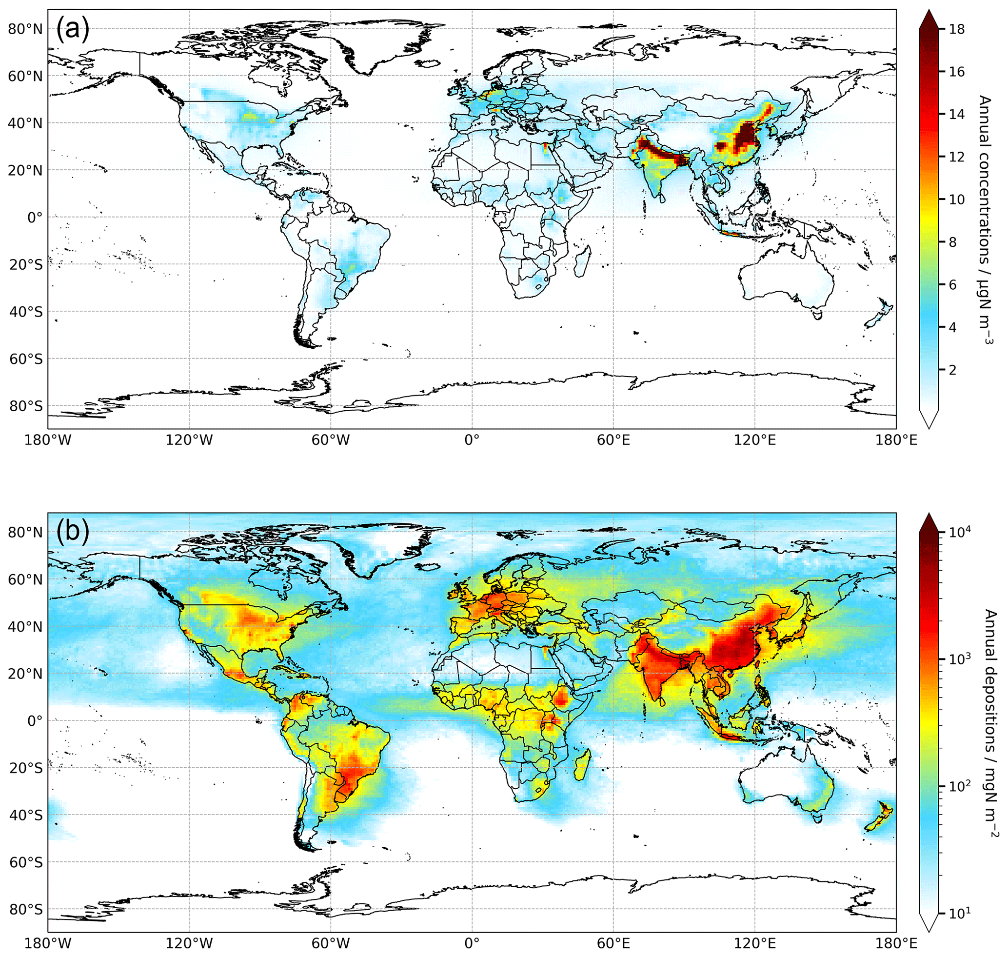
Figure 3 (a) Annual mean surface concentrations and (b) annual total (wet + dry) depositions of reduced N (${\mathrm{NH}}_{\mathrm{3}}+{{\mathrm{NH}}_{\mathrm{4}}}^{+}$) for 2010 based on the ECLIPSE_E inventory.

The influences of the two emission inventories on model simulated surface concentration differs according to consideration of the primary or secondary component and varies from one region to another. Globally, the difference in modelled area-weighted annual mean surface NH₃ concentration using the two 2010 inventories is 18 % (HTAP: 0.26 µg m⁻³; ECLIPSE_E: 0.31 µg m⁻³). The relative difference is the same when considering land-only area-weighted mean surface NH₃ concentration (0.83 and 0.99 µg m⁻³ for HTAP and ECLIPSE_E, respectively). In contrast, the difference for global area-weighted mean surface ${{\mathrm{NH}}_{\mathrm{4}}}^{+}$ concentration is only 3.5 % for ${{\mathrm{NH}}_{\mathrm{4}}}^{+}$ (HTAP: 0.316 µg m⁻³; ECLIPSE_E: 0.305 µg m⁻³) or 5.0 % for the land-only area-weighted ${{\mathrm{NH}}_{\mathrm{4}}}^{+}$ concentrations of 0.755 and 0.718 µg m⁻³, respectively.

For a regional perspective, Figs. 4 and S5 in the Supplement respectively compare the modelled NH₃ and ${{\mathrm{NH}}_{\mathrm{4}}}^{+}$ concentrations using the two emission inventories for the grids in which there are also available measurements from the monitoring networks. Considering all measurement locations globally, the model simulated concentrations using the two inventories are extremely well spatially correlated with each other at R=0.95 for NH₃ and 0.98 for ${{\mathrm{NH}}_{\mathrm{4}}}^{+}$. The average difference in global surface NH₃ concentration between model simulations using ECLIPSE_E and HTAP based on measurement locations is 0.34 µg m⁻³, which corresponds to only 15 % of the model average concentration of 2.30 µg m⁻³ using the ECLIPSE_E inventory or 17 % of the model average concentration of 1.96 µg m⁻³ using the HTAP inventory.

The model concentrations using the two emission inventories are similarly linearly correlated with measurements (Fig. 4). As discussed above, systematic differences between modelled and measured concentrations of NH₃ in East Asia and Southeast Asia can be attributed at least in part to local differences in NH₃ emissions among different inventories. The average modelled NH₃ concentrations in China derived from ECLIPSE_E and HTAP (based on measurement locations) are 12.3 and 7.9 µg m⁻³, respectively. The systematically greater modelled NH₃ concentrations using ECLIPSE_E compared to HTAP is consistent with the ECLIPSE_E inventory's larger NH₃ emissions over eastern and southern China (Fig. 2), where the majority of the NNDMN measurement sites are located (Fig. 1).

For measurement locations in Southeast Asia, Fig. 4 shows that modelled NH₃ concentrations are generally lower than their respective measured concentrations for simulations using both emissions inventories. However, as for China, model simulations of NH₃ using the two inventories are spatially well correlated with each other (R=0.92). The overall average modelled NH₃ concentration (based on grids containing EANET sites) of 1.99 µg m⁻³ using the HTAP inventory is slightly greater than the average concentration of 1.50 µg m⁻³ using the ECLIPSE_E inventory. Using the HTAP inventory also gives a slightly larger range in simulated NH₃ concentrations (0.00–9.14 µg m⁻³) for the grids with measurement sites than the range (0.01–6.54 µg m⁻³) when using the ECLIPSE_E inventory. This is again consistent with the smaller emissions for ECLIPSE_E in most southeastern Asian countries in 2010 (Fig. 2).

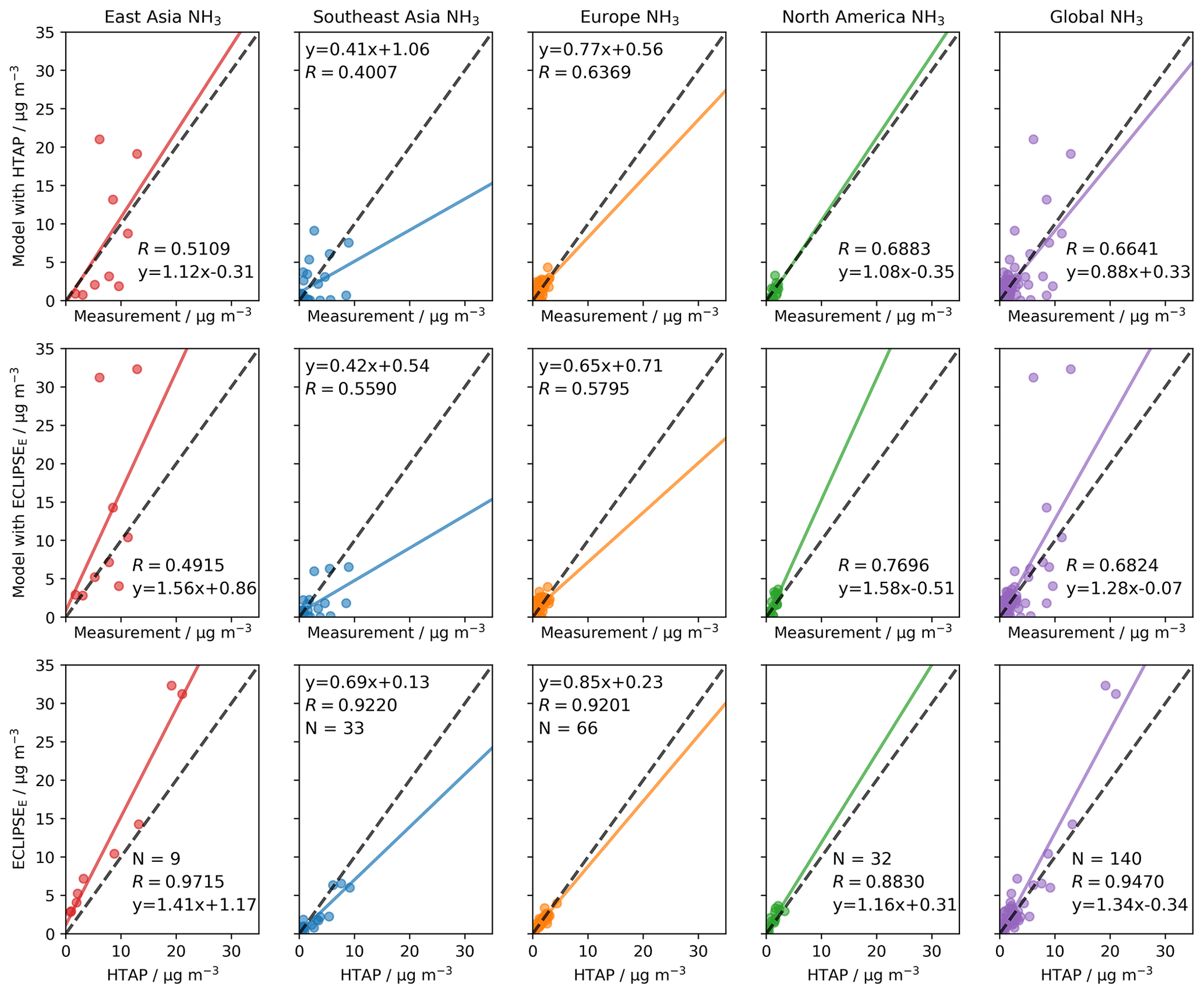
Figure 4 Comparisons of annual average surface concentrations of NH₃ for eight monitoring networks in 2010 – NNDMN from China as East Asia, EANET as Southeast Asia, NAMN and AGANet (UK) and EMEP/CCC plotted together here as Europe, and the EPA and AMoN (USA) and NAPS (Canada) plotted together here as North America – and for all networks combined (“global”). The upper row of plots is modelled versus measured values using the HTAP emission inventory. The middle row is modelled versus measured values using the ECLIPSE_E emission inventory. The lower row is the modelled data for the two inventories plotted against each other for the same set of model grids that contain measurement sites. In each plot, N is the total number of scatter points, R is the Pearson correlation coefficient, the dashed black line is the 1:1 line, and the solid coloured line is the trend line corresponding to the equation presented.

In North America and Europe there are similar linearities between the modelled and measured NH₃ concentrations when using either of the HTAP and ECLIPSE_E inventories (Fig. 4). In general, both inventories produce smaller concentrations than measurements in Europe, with ECLIPSE_E underestimating more, and higher concentrations than measurements in North America, with ECLIPSE_E overestimating more. In other words, the ECLIPSE_E inventory yields smaller NH₃ concentrations in Europe but higher concentrations in North America compared with the HTAP inventory. The differences in NH₃ emissions between the two inventories are very similar in these two regions: Fig. 2 shows that the differences in emissions are generally close to zero and that differences are both positive and negative. Therefore, it is the location of the measurement site that likely influences the model evaluation statistics. The modelled NH₃ concentrations in North America (based on network locations) are in the ranges 0.01–3.30 and 0.04–3.64 µg m⁻³ for simulations with HTAP and ECLIPSE_E inventories, respectively, while in Europe the equivalent modelled NH₃ concentration ranges are 0.00–4.36 and 0.00–3.95 µg m⁻³. The average NH₃ concentration difference (based on network locations) in North America between the two emission inventories is 0.47 µg m⁻³ (ECLIPSE_E – HTAP), whilst this difference in Europe is only 0.03 µg m⁻³.

The impact of emission inventory differences on concentrations of secondary pollutants is much smaller than for primary pollutants since the former are influenced by multiple emissions and the timescales for their formation act to smooth out spatial differentials in primary emissions. This is illustrated by the generally better agreement between model outputs for both the HTAP and ECLIPSE_E emissions inventories and the network measurements of annual ${{\mathrm{NH}}_{\mathrm{4}}}^{+}$ concentrations in Fig. S5 than for NH₃ in Fig. 4. Thus, the correlations between modelled and measured ${{\mathrm{NH}}_{\mathrm{4}}}^{+}$ at all network locations are 0.88 (range 0.54–0.92 for the four separate regions) and 0.90 (0.74–0.90) for simulations using the HTAP and ECLIPSE_E inventories, respectively, whilst the corresponding correlation coefficients for NH₃ are 0.66 (0.40–0.69) and 0.68 (0.49–0.77).

The differences in ${{\mathrm{NH}}_{\mathrm{4}}}^{+}$ concentrations in simulations using the two emission inventories (Fig. S5) are also smaller than for NH₃ (Fig. 4), as shown by concentrations that are closer to 1:1 in all regions. For example, whilst modelled NH₃ concentrations in China derived using the ECLIPSE_E inventory are on average 56 % higher than those derived using the HTAP inventory, the ${{\mathrm{NH}}_{\mathrm{4}}}^{+}$ concentrations are very similar. The annual average ${{\mathrm{NH}}_{\mathrm{4}}}^{+}$ concentrations (based on network locations) in China are 7.30 and 7.15 µg m⁻³ for HTAP and ECLIPSE_E, respectively, which is a difference of only 2 %. More detail is presented in the Supplement.

In summary, whilst there are some spatial differences in annual emissions between the HTAP and ECLIPSE_E inventories, e.g. for NH₃ emissions in China and India, emission differences on a global scale are small. The difference in global average NH₃ emissions (for 2010) is 16.0 mg m⁻² (ECLIPSE_E – HTAP), which is 14 % of the average of the HTAP and ECLIPSE_E global mean NH₃ emissions of 105 and 121 mg m⁻², respectively. The spatial heterogeneity in the positive and negative differences in emissions worldwide indicates no global difference between them. The regional differences in emissions between the two inventories impact differently on modelled surface concentrations of primary and secondary species. Both inventories yield model results that show similar linear correlations with ambient NH₃ and ${{\mathrm{NH}}_{\mathrm{4}}}^{+}$ concentration measurements and similar underestimations and overestimations in different monitoring networks. The seasonality in NH₃ emissions of HTAP and ECLIPSE_E are similar, although the latter projects greater monthly fluctuations in East Asia, Southeast Asia, and Europe, but not North America, which indicates discrepancies in temporal (monthly or day-of-week) factors applied to annual totals in different inventories.

3.1.3 Evaluation of model response to changes between 2010 and 2015 ECLIPSE_E emissions

An evaluation was also undertaken of how the modelled concentrations and depositions respond to the change in emissions in simulations using the 2010 and 2015 ECLIPSE_E emissions data, and of how these responses compared with the changes observed in the measurements between the 2 years. This analysis is presented and discussed in the Supplement. Figures S6–S9 respectively present global maps of the differences between 2010 and 2015 of the NH₃, NO_x and SO_x precursor emissions, the modelled NH₃, NO₂ and SO₂ concentrations, the modelled ${{\mathrm{NH}}_{\mathrm{4}}}^{+}$, ${{\mathrm{NO}}_{\mathrm{3}}}^{-}$ and ${{\mathrm{SO}}_{\mathrm{4}}}^{\mathrm{2}-}$ aerosol concentrations, and the modelled total depositions of reduced N, oxidized N and oxidized S. Table S1 in the Supplement quantifies the trends between 2010 and 2015 in the modelled and measured species concentrations for each regional network for those sites where measurement data are available in both 2010 and 2015. The need in this comparison for measurement sites operating in both 2010 and 2015 severely reduces the number of paired comparison data for some measurement networks.

In summary, changes in emissions of NH₃ between 2010 and 2015 ECLIPSE_E inventories are generally small (Fig. S6). The global area-weighted average NH₃ emission increases by 4.5 % from 2010 to 2015. By contrast, NO_x and SO_x emissions show slightly larger variations (Fig. S6). The global area-weighted average emissions of NO_x and SO_x decrease from 2010 to 2015 by 5.7 % and 14 %, respectively. The trends in modelled NH₃, NO₂, and SO₂ annual concentration changes between 2010 and 2015 (Fig. S7 and Table S1) are entirely consistent with the trends in the emissions supplied to the model, and in the corresponding measurements, given both the realistic uncertainties in emissions and measurements (and the small number of measurement data), and the differential influences of meteorology on concentrations between the 2 years. Most parts of the world show increased NH₃ concentrations but decreased NO₂ and SO₂ concentrations from 2010 to 2015. The impacts of emission changes on modelled concentrations of secondary pollutants (Fig. S8 and Table S1), and modelled total deposition of reduced N, oxidized N, and oxidized S (Fig. S9) are varying. The comparison of modelled and measured concentration changes based on measurement locations (Table S1) indicates that trends in modelled and measured concentrations for SO₂ and ${{\mathrm{SO}}_{\mathrm{4}}}^{\mathrm{2}-}$ in most networks from 2010 to 2015 show clear decreases, while for NH₃, ${{\mathrm{NH}}_{\mathrm{4}}}^{+}$, NO₂, HNO₃, and ${{\mathrm{NO}}_{\mathrm{3}}}^{-}$ the modelled and measured concentrations reveal a mixture of upward, downward, and no trends but are again generally consistent with each other.

Overall, these comparisons of changes in model-simulated concentration and deposition changes between the 2 years in relation to the changes in measurements (and the emissions) provide useful additional confirmation that the model is behaving in line with expectations, within realistic levels of measurement uncertainty.

3.2 Comparisons of modelled surface concentrations of N_r and SIA species with measurements

Evaluations of modelled versus measured concentrations were undertaken for both 2010 and 2015. The comparisons for the 2 years show similar characteristics. To avoid repetition, the following section presents and discusses the comparisons for 2015, using the ECLIPSE_E inventory, as more measurement data were available for 2015. Throughout this section (and only in this Sect. 3.2) the following notation is used when referring to correlation coefficients. The correlation coefficient applying to all the networks shown in a figure is denoted by R_T (T for total), whilst that for each network individually is denoted by its own subscript: R_N is for NNDMN network; R_E is for EANET network, R_EM is for EMEP/CCC network, R_UK is for UK network, R_US is for US network, and R_NA is for NAPS network.

3.2.1 East Asia and Southeast Asia

Figure 5 shows the spatial distribution of modelled and measured 2015 annual average NH₃ concentrations for regions covered by the NNDMN (China) and EANET (East Asia) networks. Scatter plots of the paired model versus measurement annual concentrations for NH₃, ${{\mathrm{NH}}_{\mathrm{4}}}^{+}$, and other gaseous- and particle-phase inorganic components are shown in Fig. 6, illustrating the extent of model–measurement spatial correlations. A summary of model evaluation statistics is presented in Table 2.

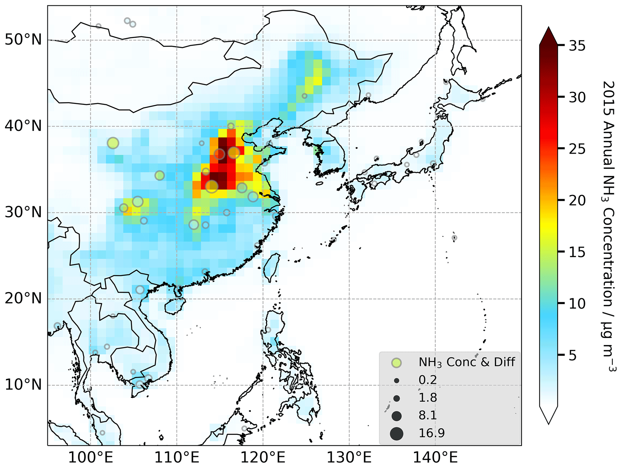
Figure 5 Modelled and measured 2015 annual mean NH₃ concentrations in East Asia and Southeast Asia. Measurements are from the China NNDMN and East Asia EANET networks. Monitoring sites are indicated by circles whose colour represents the measured concentration and whose diameter (see inset legend) represents the absolute difference between model and measurement.

Figure 6 Scatter plots of 2015 annual mean modelled and measured NH₃, NO₂, HNO₃, SO₂, ${{\mathrm{NH}}_{\mathrm{4}}}^{+}$, ${{\mathrm{NO}}_{\mathrm{3}}}^{-}$, and ${{\mathrm{SO}}_{\mathrm{4}}}^{\mathrm{2}-}$ concentrations at East Asian and Southeast Asian monitoring network locations. In each plot, the solid line is the least-squares regression line and the dashed black line is the 1:1 line. R_N is for NNDMN network. R_E is for the EANET network. R_T is the overall correlation coefficient between the model and all measurements shown.

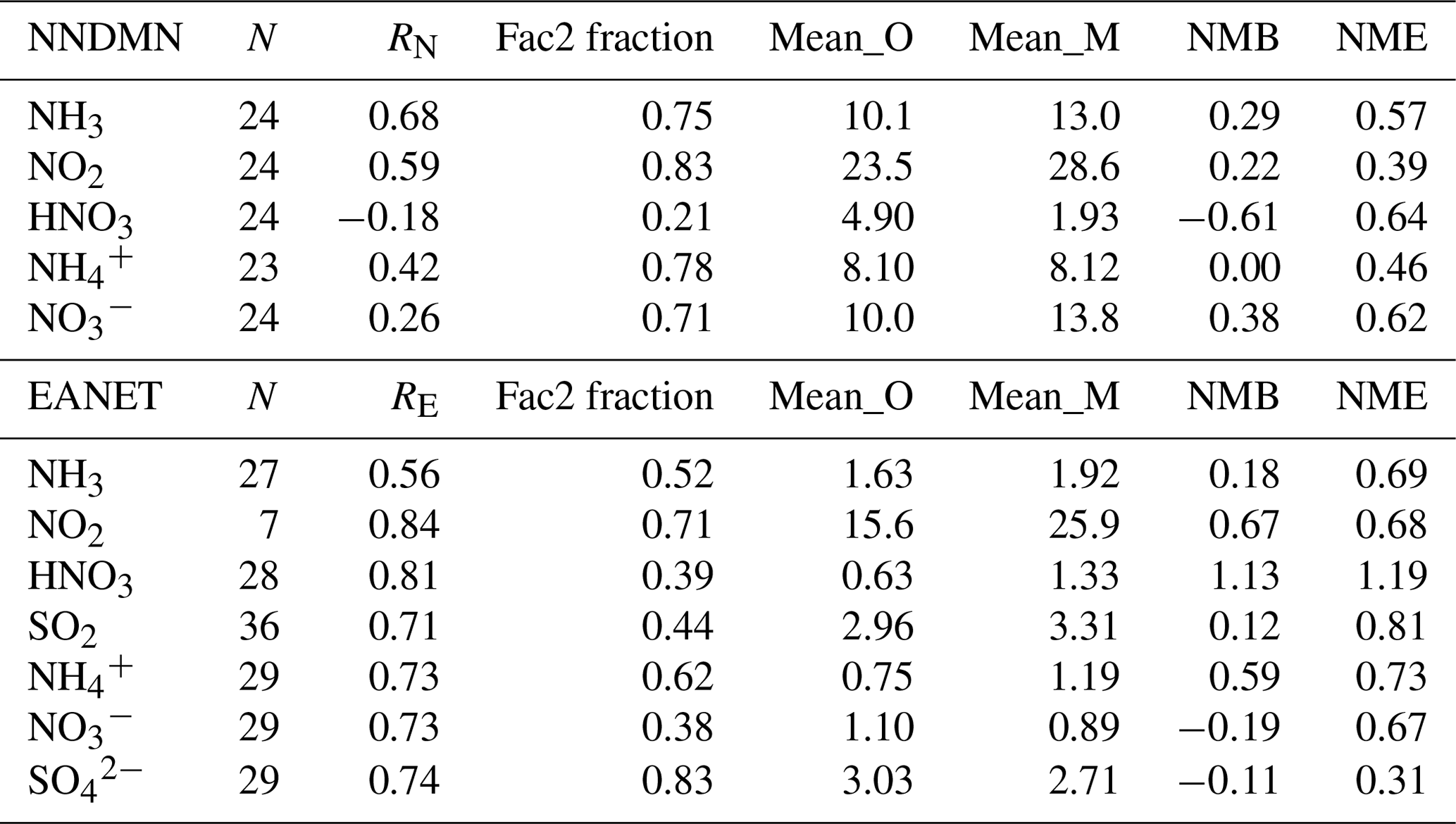
Table 2 Summary statistics of model comparison with measurements for 2015 in East Asia and Southeast Asia (NNDMN and EANET networks). N is the number of paired data of model and observation. R_N and R_E are Pearson's coefficients for NNDMN and EANET respectively. Fac2 is the fraction of data points within a factor of 2. Mean_O and Mean_M are annual average concentrations (µg m⁻³) of observation and model respectively. NMB is normalized mean bias, NME is normalized mean error.

The model simulates well the overall spatial trend of annual NH₃ concentrations in this region, spanning a range from around 0 to >30 µg m⁻³. Model and measurements consistently show highest NH₃ concentrations in central eastern China (typically >15 µg m⁻³). The observed NH₃ hotspots in North China Plain, Northeast China Plain, and Sichuan Basin are consistent with them being regions of intensive agricultural activities that apply large amounts of fertilizers (Xu et al., 2015). Most areas in other East and South-East Asia countries such as Japan, Thailand, Vietnam and Malaysia have lower NH₃ concentrations (typically <5 µg m⁻³) for both model and measurements. Relative differences between model and measurement are generally small for the majority of sampling sites, and where they are large it is a consequence of expressing a difference relative to a small measured concentration. For example, the largest relative difference of 420 %, which is in Vietnam, applies to a very small measured NH₃ concentration of 0.83 µg m⁻³.

The modelled annual NH₃ concentrations at the NNDMN locations in China are slightly higher than the measurements (NMB=0.29, Table 2), with 62 % of the sites having positive model minus measurement differences. The sampling site with the largest positive difference is Zhumadian, where modelled NH₃ exceeds the measurement by 16.9 µg m⁻³ (98 % relative to measurement). The largest negative difference (−13.0 µg m⁻³, −82 % relative to measurement) is for the Wuwei site. The large concentration differences reflect the much larger NH₃ concentrations in China. The average difference (mean bias) of annual NH₃ concentrations across all locations in the EANET network is 0.29 µg m⁻³, which is a factor of 10 smaller than the mean bias of 2.90 µg m⁻³ for the NNDMN network.

Figure 6 and Table 2 also present the statistical relationships between modelled and measured annual average concentrations in China for NO₂, ${{\mathrm{NH}}_{\mathrm{4}}}^{+}$, HNO₃ and ${{\mathrm{NO}}_{\mathrm{3}}}^{-}$. Both NH₃ and NO₂ display strong linear relationships, while the secondary species ${{\mathrm{NH}}_{\mathrm{4}}}^{+}$ and ${{\mathrm{NO}}_{\mathrm{3}}}^{-}$ show poorer correlations. The poorest agreement is for HNO₃ (Table 2). However, modelled HNO₃ concentrations agree much better with measurements in EANET and other networks (shown later), which suggests differences in measurement data among networks. Artefact-free measurement of HNO₃ is a known challenge (Tang et al., 2018b; Cheng et al., 2012; Sickles et al., 1999). The biases between model and NNDMN measurement are quite small for most species except for HNO₃. The overall annual average NH₃ concentrations are 13.0 and 10.1 µg m⁻³ for model and measurement respectively. The annual modelled network average NO₂ concentration of 28.6 µg m⁻³ is only 22 % greater than the measured network average NO₂ of 23.5 µg m⁻³. The modelled and measured network average annual mean ${{\mathrm{NH}}_{\mathrm{4}}}^{+}$ concentrations are equal at 8.1 µg m⁻³. The proportions of modelled and measured data that are within a factor of 2 are 75 % for NH₃, 83 % for NO₂, 78 % for ${{\mathrm{NH}}_{\mathrm{4}}}^{+}$, and 71 % for ${{\mathrm{NO}}_{\mathrm{3}}}^{-}$; the Fac2 for HNO₃ is, however, only 21 %.

For comparisons at EANET sites, NO₂ has the highest correlation (R_E=0.84) amongst the gaseous species, followed by HNO₃ (R_E=0.81), despite relatively higher biases between model and measurement (${\text{NMB}}_{{\mathrm{HNO}}_{\mathrm{3}}}=\mathrm{1.13}$, ${\text{NMB}}_{{\mathrm{NO}}_{\mathrm{2}}}=\mathrm{0.67}$). The linear correlations are similar for NH₃ and SO₂, and both also exhibit small biases. The network-averaged modelled and measured annual average NH₃ concentrations are 1.92 and 1.63 µg m⁻³ respectively (NMB=0.18). The equivalent data for SO₂ are 3.31 and 2.96 µg m⁻³ (NMB=0.12). For the aerosol components, the model simulates higher ${{\mathrm{NH}}_{\mathrm{4}}}^{+}$ concentrations (by 59 %), but slightly lower ${{\mathrm{NO}}_{\mathrm{3}}}^{-}$ and ${{\mathrm{SO}}_{\mathrm{4}}}^{\mathrm{2}-}$ concentrations (by 19 % and 11 %, respectively). Linear correlations of aerosol components between model and EANET measurements are high (R_E=0.73–0.74). In summary, the model shows good performance in capturing spatial variations of key inorganic pollutants at EANET locations. The comparison statistics also show an overall better model-measurement linear correlation for EANET than for NNDMN for all species.

3.2.2 Europe

The annual-mean NH₃ concentration map for Europe (Fig. 7) shows the highest NH₃ concentrations (>8 µg m⁻³) are in the Netherlands, Germany and Italy. Concentrations in northern Europe, such as Scandinavia, are smaller (<2 µg m⁻³), which is consistent with less anthropogenic activities and colder temperatures in this region. The model simulations of large NH₃ concentrations in the Po Plain in northern Italy arise from the large NH₃ emissions associated with intensive farming of pigs, cattle and poultry (Carozzi et al., 2013; Skjøth et al., 2011). In the UK, NH₃ concentrations generally display a decreasing trend from south to north for both model and measurement although Northern Ireland is a relatively high NH₃ region as well. Most sites with NH₃ concentrations around or below 1 µg m⁻³ are in northwest Scotland, where modelled NH₃ concentrations are equally low.

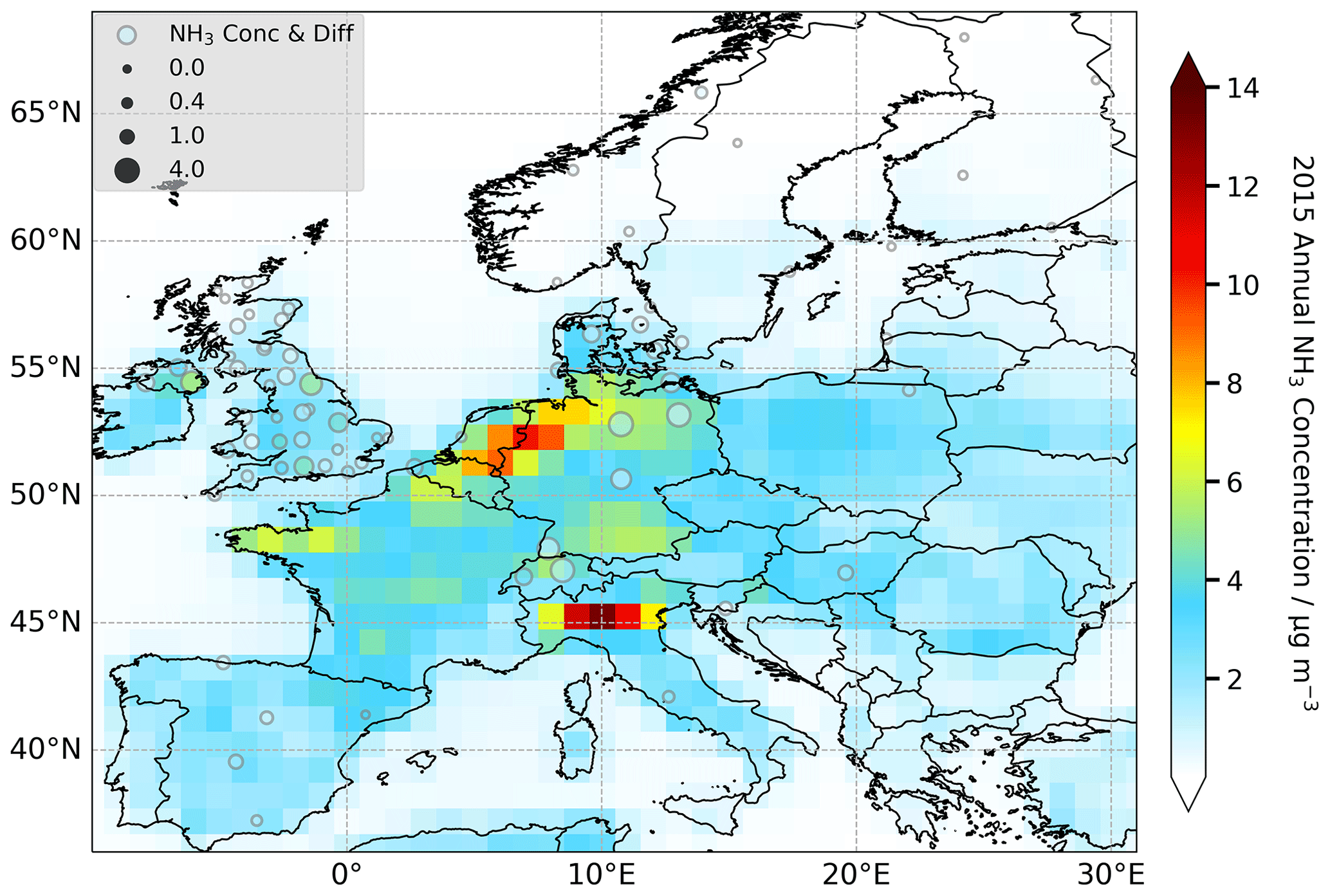
Figure 7 Modelled and measured 2015 annual mean NH₃ concentrations in Europe. Measurements are from the UK NAMN and Europe EMEP/CCC networks. Monitoring sites are indicated by circles whose colour represents the measured concentration and whose diameter (see inset legend) represents the absolute difference between model and measurement.

Across all monitoring sites in Europe, 79 % show positive differences for model minus measurement of annual NH₃. The monitoring locations with the largest differences (3.11–3.98 µg m⁻³, Fig. 7) are located in Germany and Switzerland, while most sites with differences close to zero are situated in Norway, Sweden, Finland and Scotland. The site with the largest relative difference, Rannoch in the highlands of Scotland, has an extremely low measured concentration of 0.07 µg m⁻³ relative to the modelled concentration, also low), of 1.13 µg m⁻³. A number of sites which have negative model minus measurement differences are in southern England and eastern Northern Ireland. The largest model underestimation of NH₃ (−3.18 µg m⁻³) is at the Brompton site in England which also has the highest observed NH₃ concentrations for the UK. However, it is important to note that the UK NAMN is a high spatial density NH₃ monitoring network, with many sites deliberately located near local emission sources of NH₃ (Tang et al., 2018a), which the global model grid-average cannot capture.

The linear relationships between model and measurement for 2015 annual average NH₃, NO₂, SO₂, ${{\mathrm{NH}}_{\mathrm{4}}}^{+}$, ${{\mathrm{NO}}_{\mathrm{3}}}^{-}$, and ${{\mathrm{SO}}_{\mathrm{4}}}^{\mathrm{2}-}$ concentrations in Europe are shown in Fig. 8 and a summary of the statistical comparisons is shown in Table 3. A few UK NAMN sites are part of the European EMEP/CCC network. Where a model grid contains multiple measurement sites, the average of the measured values is used.

Figure 8 Scatter plots of 2015 annual mean modelled and measured NH₃, NO₂, HNO₃, SO₂, ${{\mathrm{NH}}_{\mathrm{4}}}^{+}$, ${{\mathrm{NO}}_{\mathrm{3}}}^{-}$, and ${{\mathrm{SO}}_{\mathrm{4}}}^{\mathrm{2}-}$ concentrations at European monitoring network locations. In each plot, the solid line is the least-squares regression line and the black dashed line is the 1:1 line. R_EM is for EMEP/CCC network. R_UK is for UK networks. R_T is the overall correlation coefficient between model and all measurements shown.

Table 3 Summary statistics of model comparison with European measurements for 2015 (UK and EMEP/CCC networks). N is the number of paired data of models and observations. R_T is Pearson's coefficient for total measurements in EMEP/CCC and UK networks. Fac2 is the fraction of data points within a factor of 2. Mean_O and Mean_M are annual average concentrations (µg m⁻³) of observation and model, respectively. NMB is normalized mean bias, and NME is normalized mean error.

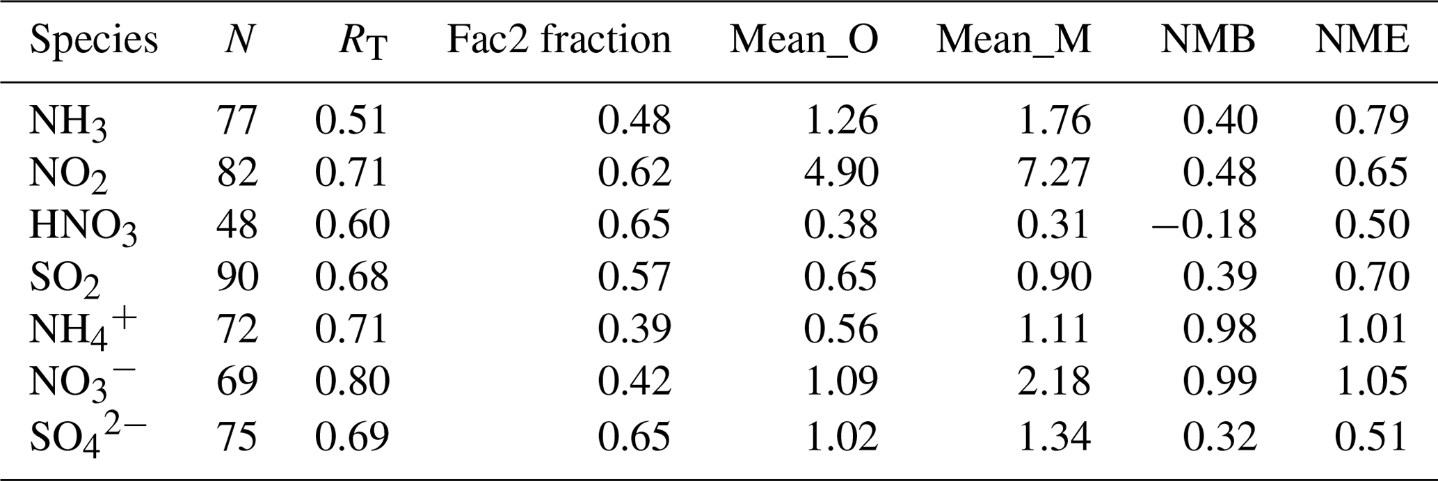
There is a clear linear correlation between model and measurement for both primary and secondary species (Fig. 8). Correlation is highest for ${{\mathrm{NO}}_{\mathrm{3}}}^{-}$ (R_T=0.80), followed by NO₂ and ${{\mathrm{NH}}_{\mathrm{4}}}^{+}$ (R_T=0.71) and weakest for NH₃ (R_T=0.51). However, the NH₃ data appear to be distributed into two groups, one characterized by positive model bias mainly associated with EMEP/CCC network locations and one characterized by negative model bias mainly associated with the UK network. The former may be a result of overestimation of NH₃ in the emission inventory, the latter may be caused by UK measurement locations adjacent to agricultural NH₃ sources (Tang et al., 2018a). The model–measurement comparisons of other gaseous species (NO₂, SO₂, and HNO₃) all show better correlations (R_T=0.60–0.71) and smaller differences (NME 0.50–0.70) in comparison with NH₃.

The modelled concentrations of secondary components, ${{\mathrm{NH}}_{\mathrm{4}}}^{+}$, ${{\mathrm{NO}}_{\mathrm{3}}}^{-}$, and ${{\mathrm{SO}}_{\mathrm{4}}}^{\mathrm{2}-}$, all match well with the spatial variations of measurements, with R_T varying from 0.69 to 0.80 (Fig. 8). All three components show higher modelled than measured concentrations to a varying degree. The network-averaged ${{\mathrm{NH}}_{\mathrm{4}}}^{+}$ concentrations are 1.11 and 0.56 µg m⁻³ for model and measurement, respectively. For ${{\mathrm{NO}}_{\mathrm{3}}}^{-}$, the modelled average concentration is 2.18 µg m⁻³, which is around twice the measurement mean. In comparison with ${{\mathrm{NH}}_{\mathrm{4}}}^{+}$ and ${{\mathrm{NO}}_{\mathrm{3}}}^{-}$, ${{\mathrm{SO}}_{\mathrm{4}}}^{\mathrm{2}-}$ shows a smaller NMB (0.32) and a larger Fac2 fraction (64 %).

In conclusion, across Europe the model exhibits a good performance in simulating annual average concentrations and spatial variations of major inorganic air pollutants, but with an overestimation of secondary ${{\mathrm{NH}}_{\mathrm{4}}}^{+}$, ${{\mathrm{NO}}_{\mathrm{3}}}^{-}$, and ${{\mathrm{SO}}_{\mathrm{4}}}^{\mathrm{2}-}$. The overall agreement between model outputs and ambient measurements in Europe networks is as good as that in EANET network.

3.2.3 United States and Canada

Modelled and measured 2015 annual average NH₃ concentrations and differences in North America are shown in Fig. 9. The Canadian NAPS network includes limited sampling sites for NH₃, and all of them are situated close to the border with the USA. Areas with the highest NH₃ concentration are located in the midwestern United States according to the model, but there are only a few measurement locations in these regions. Annual average NH₃ measurements in North America vary from 0.39 to 3.74 µg m⁻³, while the model concentrations at those locations range from 0.13 to 4.62 µg m⁻³. The model generally simulates slightly higher NH₃ concentrations than measurements: 67 % of the model–measurement differences are positive and the mean model bias is 0.48 µg m⁻³. The modelled and measured concentrations of NH₃ in North America are comparable to those in Europe and much smaller than those in East Asia.

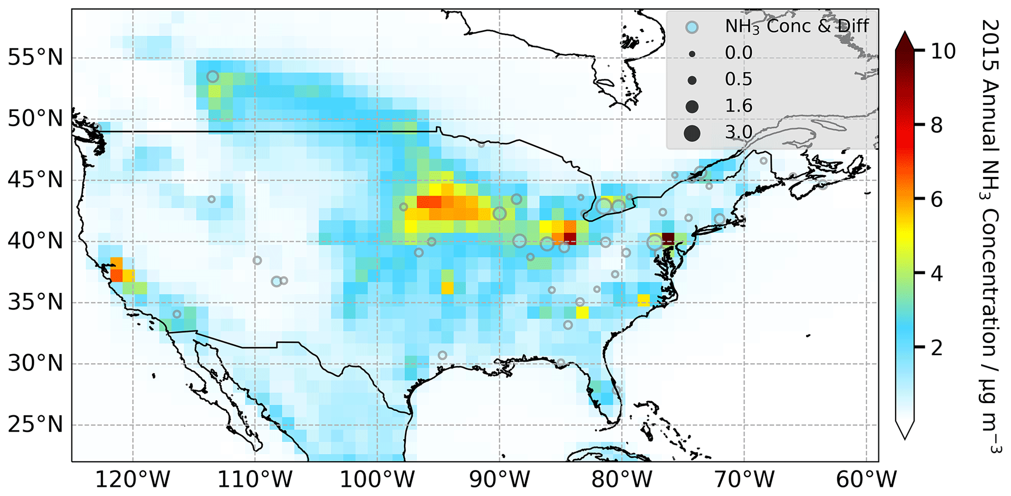
Figure 9 Modelled and measured 2015 annual mean NH₃ concentrations in North America. Measurements are from the US AMoN Network and Canada NAPS Program. Monitoring sites are indicated by circles whose colour represents the measured concentration and whose diameter (see inset legend) represents the absolute difference between model and measurement.

Figure 10 shows the linear relationships between model and measurement for 2015 annual average NH₃, NO₂, SO₂, ${{\mathrm{NH}}_{\mathrm{4}}}^{+}$, ${{\mathrm{NO}}_{\mathrm{3}}}^{-}$, and ${{\mathrm{SO}}_{\mathrm{4}}}^{\mathrm{2}-}$ in North America. Table 4 provides the summary of statistical comparison metrics. The number of monitoring locations is greater than for the networks in East Asia, Southeast Asia, and Europe. The correlations between modelled and measured annual average NH₃, NO₂, HNO₃ concentrations in North America (R_T=0.59–0.72) are similar to those in Europe and Southeast Asia, but the correlation for SO₂ is poor (R_T=0.27). The reason for the poorer correlation between modelled and measured SO₂ is unknown but may have a few causes: the emission inventory for SO₂ in North America may be too low or some sampling sites may be set close to SO₂ point sources whilst grid-averaged model values are much lower. For the other three gaseous species, the biases between model and measurement are in reasonable ranges. The network-averaged modelled NH₃ concentration is 1.76 µg m⁻³, which is close to the measured average concentration of 1.28 µg m⁻³. For HNO₃, 78 % of model data are within a factor of 2 of the measurements, and the overall average concentrations are 0.53 and 0.39 µg m⁻³ for the model and measurements, respectively (Table 4). Compared to NH₃ and HNO₃, the modelled annual NO₂ concentrations are generally smaller than measurements, leading to a negative NMB of −0.39.

Clear linear relationships are observed between modelled and measured annual average concentrations for all three aerosol pollutants (Fig. 10, Table 4), among which ${{\mathrm{SO}}_{\mathrm{4}}}^{\mathrm{2}-}$ has the highest correlation coefficient (0.86), the largest Fac2 (87 %), and the smallest NMB and NME. This reflects excellent capability by the model to capture the spatial variation of SIA constituents. In terms of absolute concentrations, modelled concentrations are on average higher than measured to varying degrees for ${{\mathrm{NH}}_{\mathrm{4}}}^{+}$, ${{\mathrm{NO}}_{\mathrm{3}}}^{-}$, and ${{\mathrm{SO}}_{\mathrm{4}}}^{\mathrm{2}-}$, as is the case in Europe. This may be due to gas-to-particle conversion process being too fast in the model or sinks of these secondary species being too small. The network-averaged ${{\mathrm{NH}}_{\mathrm{4}}}^{+}$ concentrations are 1.06 and 0.50 µg m⁻³ for model and measurement, respectively. For ${{\mathrm{NO}}_{\mathrm{3}}}^{-}$ the equivalent concentrations are 1.19 and 0.58 µg m⁻³. Both ${{\mathrm{NH}}_{\mathrm{4}}}^{+}$ and ${{\mathrm{NO}}_{\mathrm{3}}}^{-}$ show relatively small Fac2 fractions due to model overestimation. By contrast, the smallest differences are for ${{\mathrm{SO}}_{\mathrm{4}}}^{\mathrm{2}-}$ concentrations. The average model ${{\mathrm{SO}}_{\mathrm{4}}}^{\mathrm{2}-}$ concentration is 1.27 µg m⁻³, which only exceeds the average measurement concentration by 31 %.

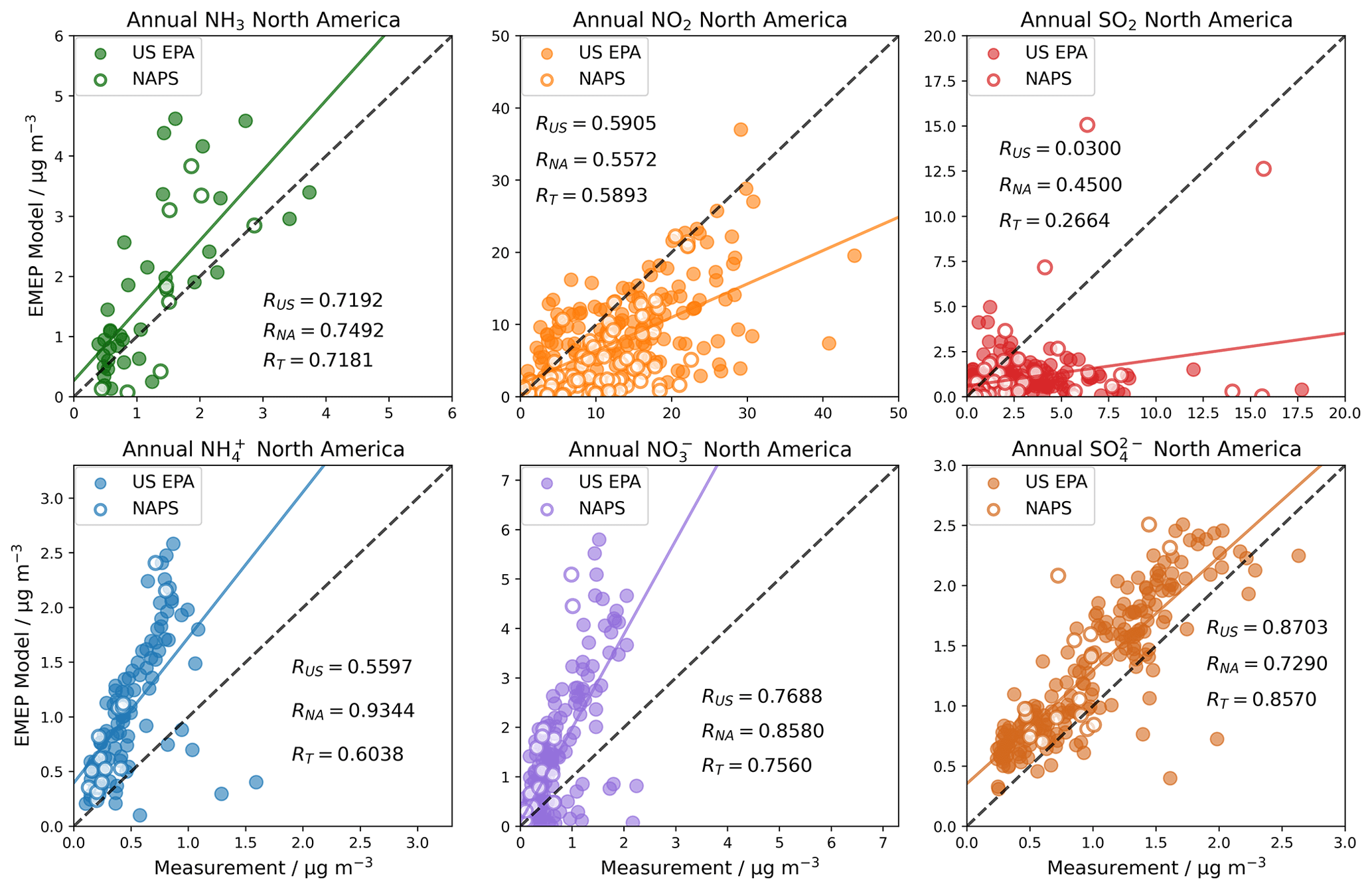
Figure 10 Scatter plots of 2015 annual mean modelled and measured NH₃, NO₂, HNO₃, SO₂, ${{\mathrm{NH}}_{\mathrm{4}}}^{+}$, ${{\mathrm{NO}}_{\mathrm{3}}}^{-}$, and ${{\mathrm{SO}}_{\mathrm{4}}}^{\mathrm{2}-}$ concentrations at North American monitoring network locations. In each plot, the solid line is the least-squares regression line and the dashed black line is the 1:1 line. R_US is for U.S. EPA network. R_NA is for NAPS network. R_T is the overall correlation coefficient between model and all measurements shown.

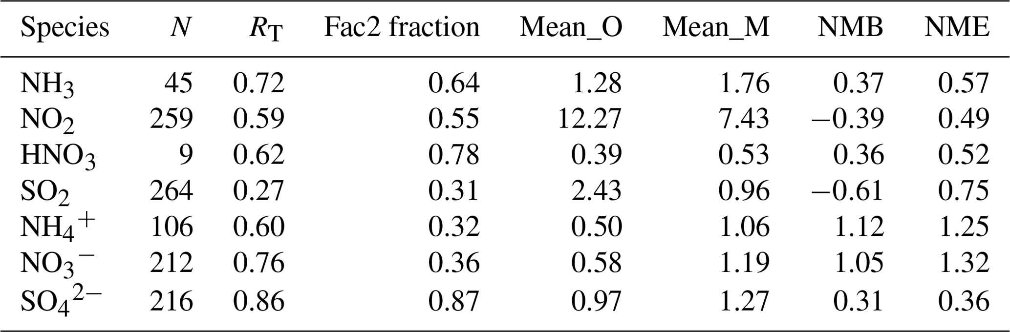
Table 4 Summary statistics of model comparison with measurements for 2015 in North America (U.S. EPA and NAPS networks). N is the number of paired data of model and observation. R_T is Pearson's coefficient for total measurements in U.S. EPA and NAPS networks. Fac2 is the fraction of data points within a factor of 2. Mean_O and Mean_M are annual average concentrations (µg m⁻³) of observation and model, respectively. NMB is normalized mean bias, NME is normalized mean error.

3.2.4 Comparison of temporal variation of modelled concentrations with measurements

The NNDMN, EANET, NAMN, and EMEP/CCC monitoring networks also provide higher temporal resolution data, which allows a comparative assessment of monthly variations in model simulations (Fig. 11). As well as model-imposed temporal variations in emissions, the NH₃ concentrations are also driven by meteorological variations, in particular warmer temperatures favour partitioning of reduced N to gaseous NH₃. Missing measurement data for certain months and sites means the number of comparisons varies from 1 month to another.

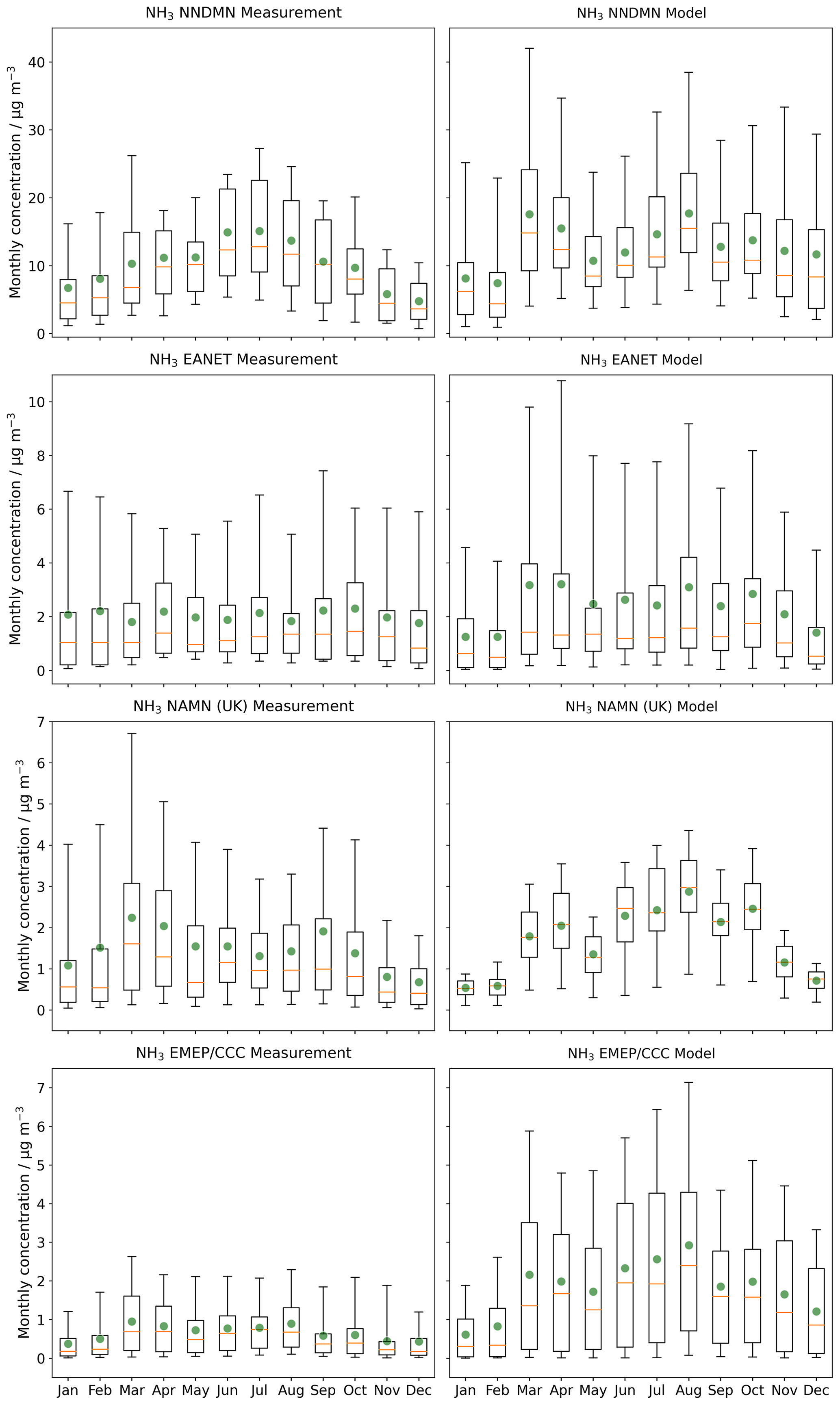
Figure 11 Monthly variations in modelled and measured NH₃ concentrations for locations in four monitoring networks in 2015. The box extends from the lower to upper quartile values of the data, with an orange line at the median and a green point at the mean. The whiskers represent 5 % and 95 % percentiles.

In general, measurements of monthly average NH₃ concentrations in the China NNDMN show a trend of high in summer (mean: 14.6 µg m⁻³, Table 5) and low in winter (mean: 6.54 µg m⁻³). The seasonal pattern in the model simulations is slightly different, with dual peaks of NH₃ concentrations in March and August, but seasonal averages for spring and summer in model are similar to summer measurements at 14.6 and 14.8 µg m⁻³, respectively. Similar to measurements, the modelled NH₃ concentration is also lowest in winter (9.09 µg m⁻³). For the EANET, both modelled and measured NH₃ median concentrations show a less clear varying trend than other networks, which might be due to the distributions of monitoring sites. A large number of sites in Southeast Asia are located in the tropics where the climate is characterized by a small temperature range and substantial rainfall, which leads to a very small range of fluctuations of NH₃ concentrations. The monthly averages indicate that measurements peak in April and October and are minimum in March and August, while the model has higher concentrations in March, April, August, and October, and lower concentrations in January and February. However, the fluctuation in the all-site monthly averages is small, ranging from 1.21 to 3.21 µg m⁻³ and from 1.77 to 2.30 µg m⁻³ for model and measurement, respectively. The variation in monthly medians is even smaller.

Table 5 Seasonal averages of monthly NH₃ concentrations (µg m⁻³) for model (Mod) and measurements (Obs) in four monitoring networks: spring, i.e. March, April, May; summer, i.e. June, July, August; autumn, i.e. September, October, November; winter, i.e. December, January, February.

For the UK NAMN, both mean and median concentrations (Fig. 11) show that models and measurements exhibit higher NH₃ concentrations in spring and summer, and lower concentrations in winter. One small difference is in the timing of the NH₃ concentration maximum. The highest measured NH₃ concentrations are in spring, whereas modelled concentrations have a maximum in summer. The differences between all-site monthly mean and median concentrations and between the maximum and minimum values in the measurements are much larger than in the model, indicating a broad sub-grid variability that cannot be captured by the global model as the spatial averaging process smooths out these highly localized concentration gradients. For the European EMEP/CCC network, the model is in excellent agreement with measurement in respect to temporal pattern despite its higher absolute concentrations. Both model and measurement show a continuous period of higher NH₃ concentrations from spring to summer and lower NH₃ concentrations in autumn and winter.

Similar model–measurement monthly comparisons for ${{\mathrm{NH}}_{\mathrm{4}}}^{+}$ in 2015 are presented in the Supplement (Fig. S10). Consistent monthly patterns are observed for both model and measurements in the EANET, AGANet (UK), and EMEP/CCC networks: larger ${{\mathrm{NH}}_{\mathrm{4}}}^{+}$ concentrations are found in February, March, and October, while the lowest concentration appears in July. For NNDMN locations, the model and measurement show a similar late summer peak but display an inverse trend in winter and spring.

In summary, the simulated concentrations of NH₃ and ${{\mathrm{NH}}_{\mathrm{4}}}^{+}$ and their month-to-month variability are generally in line with measurement data in most global regions despite the model resolution of $\mathrm{1}{}^{\circ }\times \mathrm{1}{}^{\circ }$. The model comparisons with European measurements exhibit greater agreements than with East Asian and Southeast Asian measurements. The divergence in NNDMN and EANET likely comes from shortcomings in the temporal profiles of emission inventories and is affected by the distribution of limited measurement sites. A comparison of model outputs from STOCHEM-CRI and WRF-Chem-CRI with satellite observations (Khan et al., 2020) also highlights a poor temporal agreement for NH₃ seasonality. Further model experiments are required to investigate the impacts of different monthly emission and local meteorology on temporal variations of reduced N species.

3.3 Comparisons of modelled precipitation and wet deposition with measurements

The evaluations of model performance for precipitation and wet deposition are based on the four monitoring networks (China, East Asia, Europe, and the United States) that report both precipitation and precipitation concentration measurements for 2015. The total annual wet deposition (WDEP) is calculated as follows:

$$\text{WDEP}=\stackrel{\mathrm{‾}}{C}\times \sum P_i,$$

where $\stackrel{\mathrm{‾}}{C}$ (also referred to here as Prec Conc) is the precipitation-weighted annual average concentration

$$\stackrel{\mathrm{‾}}{C}={\displaystyle \frac{\sum (C_i\times P_i)}{\sum P_i}},$$

C_i is the concentration, and P_i is the depth of each individual precipitation event i in the year. Prec Amount, ∑P_i, is the total precipitation depth for the year. When C_i (and $\stackrel{\mathrm{‾}}{C}$) are expressed in units of milligrams per litre and P_i in millimetres, then WDEP is expressed in units of milligrams per square metre.

Figure 12 shows for each location in each of the five networks the comparisons between modelled and measured annual precipitation, precipitation-weighted annual average concentration of reduced N (in the form of ${{\mathrm{NH}}_{\mathrm{4}}}^{+}$) and annual total wet deposition of reduced N in 2015. Table 6 summarizes the statistical metrics associated with each comparison. The comparisons of modelled and measured total rainfall show that the model is capable of simulating spatial variations of precipitation over different global regions. The correlation coefficient R between modelled and measured annual precipitation ranges from 0.65 to 0.94 with an average of 0.77. The high Fac2 proportions indicate that the model can simulate the precipitation amount in EANET (82 %), EMEP/CCC (91 %), US NTN (82 %), and Canada CAPMoN (100 %) locations but not so well for NNDMN (43 %). In terms of model–measurement biases, the model underestimates annual precipitation amounts by 13 %–45 %. Given the 1^∘ spatial resolution of the model and the localized nature of precipitation events, such a model underestimation range is expected.

The model performance in precipitation concentrations of reduced N varies between NNDMN and other networks. Whilst comparisons for EANET, EMEP/CCC, US NTN, and Canada CAPMoN show close to 1:1 linear relationships with R values all >0.71, comparison at NNDMN locations shows a relatively poor correlation (R=0.45). This may reflect instrumental and experimental differences between monitoring networks. Considering the limited number of monitoring sites in NNDMN, more measurement data are required to draw a more representative model–measurement comparison in China.

The measured annual wet deposition of reduced N is affected by the quality of the measurement of both collected rainfall and precipitation-weighted average ${{\mathrm{NH}}_{\mathrm{4}}}^{+}$ concentration. Based on measurement locations, NNDMN shows the largest annual reduced N wet deposition for both model (777 mg N m⁻²) and measurement (986 mg N m⁻²), followed by EANET (model 380 mg N m⁻², measurement 499 mg N m⁻²), EMEP/CCC (model 146 mg N m⁻², measurement 226 mg N m⁻²), Canada CAPMoN (model 144 mg N m⁻², measurement 288 mg N m⁻²), and US NTN (model 135 mg N m⁻², measurement 192 mg N m⁻²). The model simulates lower total reduced N wet depositions by 21 %–50 % across the five networks. This general model underestimation is largely driven by the underestimation of total precipitation, and to less extent the precipitation concentration. Across the five networks, linear correlation between modelled and measured wet deposition of reduced N is best for the Canada CAPMoN network with R=0.82.

The comparison for global wet deposition of total oxidized N (in the form of ${{\mathrm{NO}}_{\mathrm{3}}}^{-}$) exhibits similar results and is presented in the Supplement (Fig. S11 and Table S2). The modelled precipitation-weighted concentrations of ${{\mathrm{NO}}_{\mathrm{3}}}^{-}$ has relatively good agreements with measurements in EANET, EMEP/CCC, US NTN, and Canada CAPMoN networks with R ranging from 0.69 to 0.82, while the comparisons in NNDMN show a poorer linear correlation between model and measurement (R=0.39). In terms of biases, the model tends to simulate higher ${{\mathrm{NO}}_{\mathrm{3}}}^{-}$ concentrations in precipitations in EANET (NMB=0.52) and US NTN (NMB=1.04) networks but underestimate in NNDMN ($\text{NMB}=-\mathrm{0.37}$). In general, the greatest model–measurement agreement for oxidized N wet deposition is found in Canada CAPMoN and US NTN, followed by EMEP/CCC and EANET, and to the lowest extent NNDMN, which again suggests systematic differences between monitoring networks rather than issues with the modelling of atmospheric chemistry and meteorology.

On the whole, the modelled reduced and oxidized N show similar linear relationships with measurements in precipitation and wet deposition in all regions, which further supports the utilization of the WRF and EMEP MSC-W modelling system to investigate N_r processes globally.

Table 6 Summary statistics of model comparison with measurements for annual precipitation (Prec Amount, mm), precipitation-weighted mean concentration of ${{\mathrm{NH}}_{\mathrm{4}}}^{+}$ (Prec Conc, mg N L⁻¹), and wet deposition of reduced N (WDEP, mg N m⁻²) in 2015. N is the number of measuring sites. R is Pearson's coefficient. Fac2 is the fraction of data points that are within a factor of 2. Mean_O and Mean_M of Prec Conc are annual averages of observation and model, respectively. Mean_O and Mean_M of Prec Amount and WDEP are annual totals. NMB is normalized mean bias, and NME is normalized mean error.

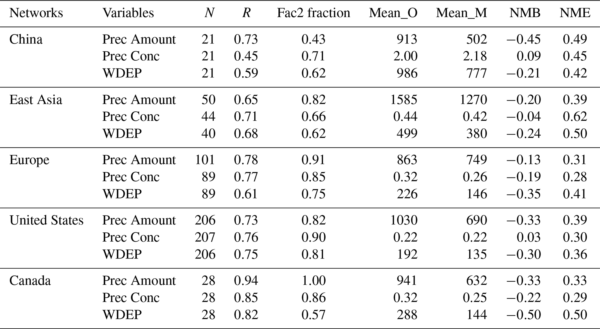
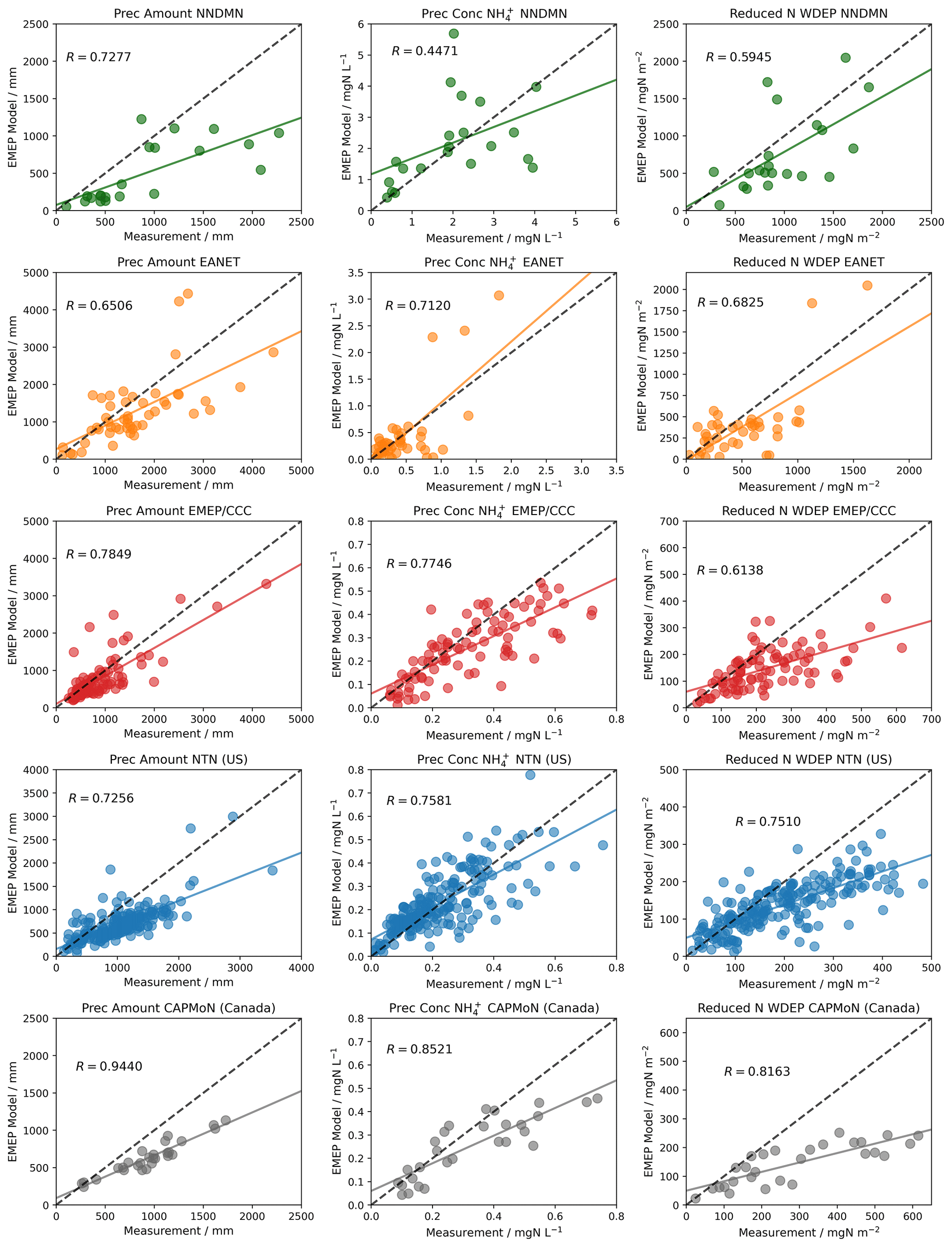
Figure 12 Scatter plots of model–measurement comparisons of 2015 annual wet deposition variables for reduced N (in the form of ${{\mathrm{NH}}_{\mathrm{4}}}^{+}$) for five measurement networks: NNDMN, EANET, EMEP/CCC, US NTN, and Canada CAPMoN. The left column shows annual precipitation. The middle column shows precipitation-weighted annual average ${{\mathrm{NH}}_{\mathrm{4}}}^{+}$ concentration in precipitation. The right column shows annual total wet deposition of ${{\mathrm{NH}}_{\mathrm{4}}}^{+}$. In each plot, the coloured line is the least-squares regression, and the dashed black line is the 1:1 line.

4 Discussion

The work presented here is motivated by the use of the EMEP MSC-W-WRF model for global-scale analyses of atmospheric nitrogen and SIA chemistry, fluxes, and budget, particularly species that contain reduced N (i.e. gaseous NH₃ and particulate ${{\mathrm{NH}}_{\mathrm{4}}}^{+}$). The model evaluation, conducted both spatially and temporarily, is based on the available data in 2010 and 2015 from nine monitoring networks that span the range of ambient measurements in East Asia, Southeast Asia, Europe, and North America.

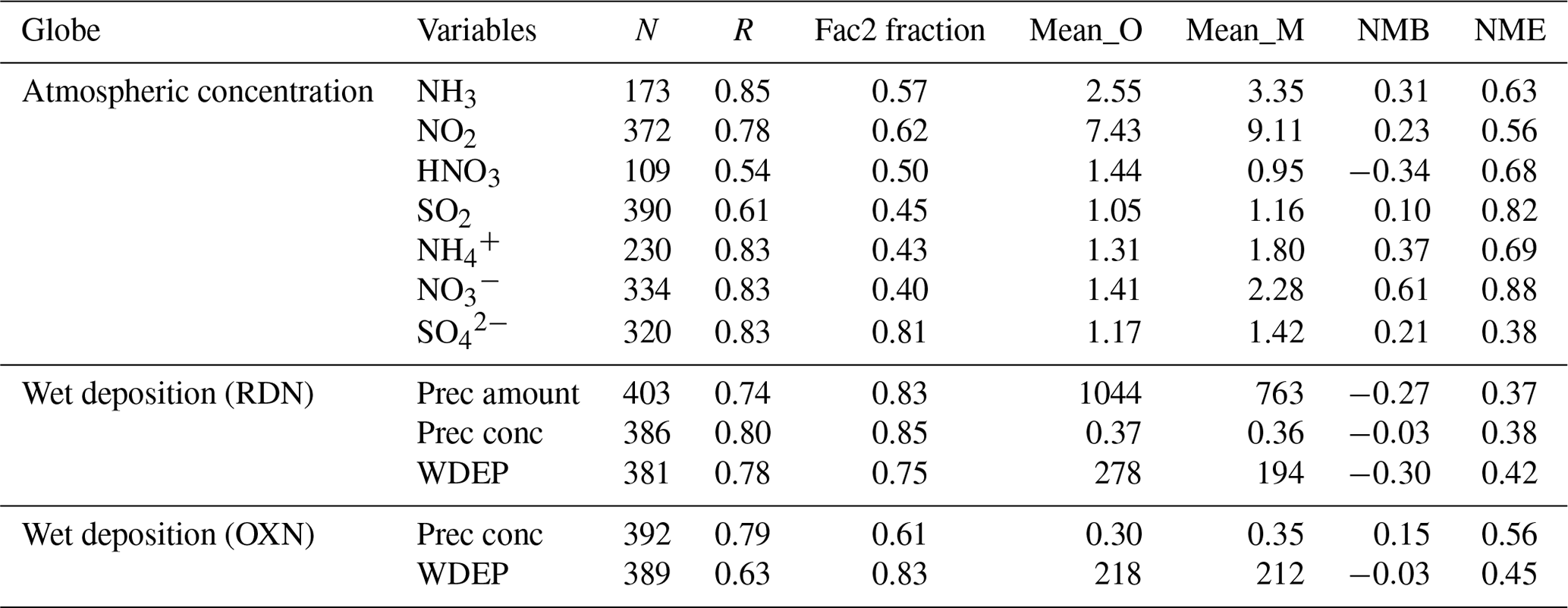
Table 7 summarizes the global comparison between model and surface measurements in 2015. The correlation coefficients (R) between modelled and measured concentrations of most species (i.e. NH₃, NO₂, ${{\mathrm{NH}}_{\mathrm{4}}}^{+}$, ${{\mathrm{NO}}_{\mathrm{3}}}^{-}$, and ${{\mathrm{SO}}_{\mathrm{4}}}^{\mathrm{2}-}$) are all greater than 0.78 except for HNO₃ and SO₂. The correlation coefficient for wet deposition of reduced N and oxidized N is 0.78 and 0.63, respectively. For reduced N species, the evaluation shows that the model overestimates NH₃ and ${{\mathrm{NH}}_{\mathrm{4}}}^{+}$ worldwide with a NMB of 31 % and 37 %, respectively. For oxidized N species, the NMB values for NO₂ and ${{\mathrm{NO}}_{\mathrm{3}}}^{-}$ are 23 % and 61 %, and in contrast HNO₃ is underestimated by 34 %. Slightly higher concentrations are also simulated by the model worldwide for both SO₂ and ${{\mathrm{SO}}_{\mathrm{4}}}^{\mathrm{2}-}$ with a NMB of 10 % and 21 %, respectively. For wet deposition, the model outputs smaller values on average for reduced N ($\text{NMB}=-\mathrm{30}\mathit{\%}$) compared with measurements, whereas the NMB for oxidized N is only −3 %. Given the intrinsic discrepancies between local site measurement and a global-scale chemistry model grid, these comparisons are good and are comparable with model evaluation statistics determined for models of similar resolution (Hauglustaine et al., 2014; Bellouin et al., 2011; Pringle et al., 2010; Xu and Penner, 2012).

Table 7 Summary statistics of global model evaluation of atmospheric concentrations (µg m⁻³), annual precipitation (Prec Amount, mm), precipitation-weighted mean concentration of ${{\mathrm{NH}}_{\mathrm{4}}}^{+}$ and ${{\mathrm{NO}}_{\mathrm{3}}}^{-}$ (Prec Conc, mg N L⁻¹), and wet deposition (mg N m⁻²) of reduced N (RDN) and oxidized N (OXN) in 2015. N is the number of measuring sites. R is Pearson's correlation coefficient. Fac2 is the fraction of data points that are within a factor of 2. Mean_O and Mean_M of Prec Conc are annual averages of observation and model, respectively. Mean_O and Mean_M of Prec Amount and WDEP are annual totals. NMB is normalized mean bias, NME is normalized mean error.

Both model and measurement have uncertainty that constrains the extent to which statistical analyses between modelled and measured data can be utilized to assess a model's performance. A reliable evaluation of a model requires a high quality of measurement as well. For instance, sampling and chemical analysis procedures such as the instrument calibration, the choice of sampling filters/tubes, the storage, extraction, and chemical speciation of air samples all have different uncertainties propagated to the final measured variable. In particular, this study and the above-mentioned global modelling studies all show difficulties in representing surface ${{\mathrm{NO}}_{\mathrm{3}}}^{-}$ and ${{\mathrm{NH}}_{\mathrm{4}}}^{+}$ concentrations, which are currently overestimated by around a factor of 2 in Europe and North America. Such positive biases between modelled and measured ${{\mathrm{NO}}_{\mathrm{3}}}^{-}$ and ${{\mathrm{NH}}_{\mathrm{4}}}^{+}$ are speculated to be partially associated with negative sampling artefacts in measurements as evaporation of NH₄NO₃ from sampling filters has been reported to cause losses of up to 50 % in summer conditions (Hauglustaine et al., 2014; Vecchi et al., 2009; Yu et al., 2005). Further work is required to better characterize and quantify the uncertainty of individual ${{\mathrm{NO}}_{\mathrm{3}}}^{-}$ and ${{\mathrm{NH}}_{\mathrm{4}}}^{+}$ measurements. In general, the relative measurement uncertainty increases markedly as concentration decreases (Thunis et al., 2013; Pernigotti et al., 2013). The EMEP/CCC data report for 2015 estimates a combined sampling and chemical analysis uncertainty range of 15 %–25 % (Hjellbrekke, 2017), while the detailed uncertainty information in other monitoring networks is not publicly available.

Similarly, different input, configurations and computing processors also have influences on the model output, and the quantification of such influence is rather complicated (Kong et al., 2020). The choice of emission input is a good example (Aleksankina et al., 2019). The compilation of an emission inventory is partially based on reported measurement data and partially on expert estimation, which consequently leads to a certain uncertainty in emission magnitudes and temporal profiles (EMEP/EEA, 2019; Hilde Fagerli, 2017; Klimont et al., 2017; Wiedinmyer et al., 2011; Zheng et al., 2012). The completeness and consistency of submitted emission data differs significantly across countries as well. As discussed in Sect. 3.1, the two global emission inventories used in this work, HTAP and ECLIPSE_E, have shown large localized discrepancies in NH₃, NO₂, and SO₂ emissions in certain world regions, which is presumably ascribable to the inclusion or exclusion of a particular local point source in the compilation process. The influence of these discrepancies on model-simulated surface concentration differs in terms of primary or secondary component and varies from one region to another, although such greatly localized influences are diminished during the spatial averaging processes. It is therefore important to acknowledge that the performance of any model is subject to the quality of model input data, which includes not only emissions but also meteorology and other aspects of model parameters. Moreover, no one can guarantee error-free models; in the same way that observations are likely to be not error free. Often in the atmospheric modelling community these potential model errors are not discussed or acknowledged.

Aside from intrinsic uncertainties in model and/or measurement values, the model and measurement may also not agree concerning the averaging time periods and the diameters of the sampled particles. A certain number of measurements may be missing from a time series due to unpredictable instrument failure and/or because the measurement averaging period does not exactly match the model averaging time period. It is clear that the sampling time and size distributions of measurements vary from one monitoring network to another and from species to species. For example, in Canada, ${{\mathrm{NH}}_{\mathrm{4}}}^{+}$ concentrations within PM_2.5 are measured, while the particle size cut-off for the DELTA system used in the UK and China is around 4.5 µm (Tang et al., 2018a, b; Xu et al., 2019). The modelled ${{\mathrm{NH}}_{\mathrm{4}}}^{+}$, ${{\mathrm{SO}}_{\mathrm{4}}}^{\mathrm{2}-}$, and fine ${{\mathrm{NO}}_{\mathrm{3}}}^{-}$ are all in PM_2.5. Another example is that in the US and Canada gaseous species like NO₂ and SO₂ are monitored continually throughout the year and thus the corresponding annual average concentrations are calculated in the same way as the model, whilst the aerosol components such as ${{\mathrm{NO}}_{\mathrm{3}}}^{-}$ and ${{\mathrm{NH}}_{\mathrm{4}}}^{+}$ are measured once per 6 d (or once per week). In addition, different networks, and even different sites in the same network, may measure at different frequencies and at different times, which presents inherent practical difficulties in comparing model simulations with ambient measurements. Further moves towards global standardized approaches for measurements across different networks is encouraged.

Even if both model and measurement were perfect representations, there still would not be complete agreement because a measurement is for a single point in space, whereas even for models with high spatial resolution, model output is a volume average. For a global model simulation with grid resolution of $\mathrm{1}{}^{\circ }\times \mathrm{1}{}^{\circ }$, the monitoring site simply samples the air in one part of that grid volume and at a specific height above the ground, which may often not reflect the average concentration for the grid. Indeed, there are particular monitoring sites where measurements are exceedingly affected by local sources. The UK NAMN is a good example, in which quite a few sites are purposely set near agricultural sources and therefore yield higher NH₃ concentrations than model grid-average predictions. The U.S. EPA also has many monitors set up next to roads with heavy traffic and hence observed much higher SO₂ levels. The representativeness of an urban (or rural) site for the air in the corresponding model grid will therefore depend on the relative size of that specific urban (or rural) area within that model grid.

The intention here is to provide an overview of how the EMEP-WRF model–measurement agreements vary among different monitoring networks and among different chemical species for evaluation of a chemistry transport model in a global context. In general, the model shows better linear correlations with surface concentration measurements in East Asia ($\stackrel{\mathrm{‾}}{R}=\mathrm{0.73}$ over seven species), Europe ($\stackrel{\mathrm{‾}}{R}=\mathrm{0.67}$ over seven species), and North America ($\stackrel{\mathrm{‾}}{R}=\mathrm{0.63}$ over seven species) than in China ($\stackrel{\mathrm{‾}}{R}=\mathrm{0.35}$ over five species). More specifically, comparisons in China show the model performs better in computing concentrations of primary pollutants (i.e. NH₃ and NO₂) than secondary species (i.e. ${{\mathrm{NH}}_{\mathrm{4}}}^{+}$ and ${{\mathrm{NO}}_{\mathrm{3}}}^{-}$), while the model evaluation statistics in East Asia, Europe, and North America show almost equally good results over all species. This implies potential discrepancies in the measurements or emissions in China rather than general issues with meteorological and atmospheric chemistry modelling. The values of statistical metrics in this work are as good as other global model evaluation studies. A global model aerosol simulation study (Hauglustaine et al., 2014) reported that the R of global model results (LMDz-INCA global chemistry–aerosol–climate model, 1.9^∘ latitude × 3.75^∘ longitude resolution) versus measurements in 2006 for surface concentrations of ${{\mathrm{SO}}_{\mathrm{4}}}^{\mathrm{2}-}$, ${{\mathrm{NH}}_{\mathrm{4}}}^{+}$ and ${{\mathrm{NO}}_{\mathrm{3}}}^{-}$ ranged from 0.43 to 0.58 in Europe and from 0.54 to 0.77 in North America, which is similar to our results presented here. The AeroCom phase III global nitrate experiment, which includes nine models, reported slightly lower R ranges than here for annual ${{\mathrm{NO}}_{\mathrm{3}}}^{-}$ in 2008: 0.081–0.735 in North America, 0.393–0.585 in Europe, and 0.226–0.429 in Southeast Asia (Bian et al., 2017); and the agreements between model and observation for gas tracers in that study were even lower than here.

This work has utilized the EMEP MSC-W v4.34 coupled with WRF v3.9.1.1 model. As discussed above, model–measurement comparison statistics will vary in different global models to different extent. However, the broad discussions associated with fundamental differences between localized measurement and grid-volume-averaged model output, inconsistent temporal coverage, relatively high uncertainties of emissions, and intrinsic limitations of measurement are generalizable, as atmospheric chemistry and transport models and other climate models are constructed similarly. Allowance for these inherent model–measurement discrepancies and uncertainties yield significantly less stringent requirements on acceptable model evaluation statistics than might initially be expected. Urban dispersion models (Denby et al., 2020; Hood et al., 2018) with higher resolutions have stronger capabilities of representing point sources and concentration gradients but are constrained even more by the accuracy of localized emission inventories and boundary conditions in the meantime, and therefore are only configured at an individual urban area. Global-scale model simulation as presented here, in spite of acknowledged limitations on coarser spatial resolution, has the advantage of generating self-consistent chemistry fields and competence for investigating contemporary and potential future global reactive nitrogen and SIA atmospheric chemistry and their regional variations.

5 Conclusions

This model versus measurement study is motivated by the first application of a global version of the EMEP MSC-W model with WRF meteorology ($\mathrm{1}{}^{\circ }\times \mathrm{1}{}^{\circ }$ horizontal resolution) to study global reactive N and S chemistry and deposition. A comprehensive spatial and temporal comparison of model output against 10 monitoring networks from four world regions (East Asia, Southeast Asia, Europe, and North America) has been undertaken, with a focus on the atmospheric concentrations and wet deposition of major inorganic pollutants and on reduced nitrogen components in particular. Simulations were performed with EMEP MSC-W model version 4.34 with WRF 3.9.1.1 meteorology, using both ECLIPSE_E (2010 and 2015) and HTAP (2010 only) emission inventories; ECLIPSE_E refers to ECLIPSE annual emissions with EDGAR monthly profiles.

In general, simulations of annual surface concentrations of a primary pollutant such as NH₃ are somewhat sensitive to the choice of HTAP or ECLIPSE_E emission inventories in places where regional differences in primary emissions between the two emission inventories are apparent, e.g. China. By comparison, the impact of difference between the emissions inventories on concentrations of secondary species such as ${{\mathrm{NH}}_{\mathrm{4}}}^{+}$ is much smaller. The difference in 2010 global area-weighted annual average NH₃ concentration is 0.05 µg m⁻³ (HTAP: 0.26 µg m⁻³; ECLIPSE_E: 0.31 µg m⁻³), which is 18 % of the absolute concentration, whilst the ${{\mathrm{NH}}_{\mathrm{4}}}^{+}$ concentration difference is only 0.02 µg m⁻³ or only 3.5 % of the global average concentrations (HTAP: 0.316 µg m⁻³; ECLIPSE_E: 0.305 µg m⁻³). In terms of temporal profiles, the monthly average emissions vary similarly throughout the year in the four world regions after the monthly profiles derived from EDGAR are applied to the ECLIPSE annual total emissions.

Comparisons of 2010 and 2015 annual average concentrations between model and measurement demonstrate that the model captures the overall spatial and temporal variations of major inorganic pollutants well despite spanning large concentration ranges in different world regions. The discussion of model evaluation statistics mainly focuses on 2015 as the results for 2010 are similar.

In general, capturing correlation is more important than bias given the intrinsic discrepancies and uncertainties between the modelled and measured variables. In this work the model shows better linear correlations with measurement networks in Southeast Asia (Mean R for seven species: $\stackrel{\mathrm{‾}}{R_{\mathrm{7}}}=\mathrm{0.73}$), Europe ($\stackrel{\mathrm{‾}}{R_{\mathrm{7}}}=\mathrm{0.67}$), and North America ($\stackrel{\mathrm{‾}}{R_{\mathrm{7}}}=\mathrm{0.63}$) than in China ($\stackrel{\mathrm{‾}}{R_{\mathrm{5}}}=\mathrm{0.35}$ over five species), which implies potential discrepancies with some measurements and emissions rather than issues with modelling meteorological and atmospheric chemistry processes. Model–measurement bias varies from one species to another in different networks. ${{\mathrm{NH}}_{\mathrm{4}}}^{+}$ and ${{\mathrm{NO}}_{\mathrm{3}}}^{-}$ are the species overestimated the most by the model in Europe and North America but not so much in East Asian and Southeast Asian networks, reflecting that the model production of the two species might be too fast and/or the chemical and physical losses might be too slow in the two regions. The model performs the best in simulating ${{\mathrm{SO}}_{\mathrm{4}}}^{\mathrm{2}-}$ concentrations in North America regarding overall statistics among various species in all networks.

Both model and measurement exhibit higher NH₃ concentrations in spring and summer, and lower concentrations in winter. The greatest agreement of temporal profile for model and measurement is found in Europe. The fluctuation of monthly average NH₃ concentrations in Southeast Asia throughout the year 2015 is fairly small for both model and measurement and the temporal trend is therefore less clear. Small differences appear regarding the specific peak concentration months in China and UK. Measurements in China show highest monthly concentration in July, while the model simulates two peaks in August and March. The highest NH₃ concentrations in the UK network are in spring, whereas the modelled concentrations peak in summer. Such disagreements again reflect the likelihood that the major driver of model discrepancies is the inaccuracy of temporal profiles of emissions rather than the simulation of atmospheric chemistries and physics.

The evaluation of wet deposition shows that the model is capable of simulating spatial variation of annual precipitation correctly in all four world regions (0.65–0.94 R range) despite a 13 %–45 % underestimation. Given that the spatial and temporal averaging smooths out highly localized effects of precipitation event, such model–measurement discrepancy is reasonable. In respect of the weighted precipitation concentrations, high linear correlations between measured and modelled ${{\mathrm{NH}}_{\mathrm{4}}}^{+}$ and ${{\mathrm{NO}}_{\mathrm{3}}}^{-}$ concentrations are observed in Southeast Asia, Europe, and North America but not China, which may again suggest a systematic difference among measurements rather than models. In general, the model shows the greatest consistency of annual total wet deposition with measurements in North America (R: 0.75–0.82 and 0.81–0.81 for reduced and oxidized N, respectively), followed by Southeast Asia (R: 0.68 and 0.51), Europe (R: 0.61 and 0.64), and China (R: 0.59 and 0.13).

Despite discussed limitations in model-measurement comparisons, the detailed evaluations presented here support the utilization of this global implementation of the EMEP MSC-W-WRF coupled model for analyses of surface concentrations and wet depositions of major reactive N and S species in different world regions. Modelling of atmospheric chemistry and transport on the global scale has the advantage of providing consistent data with comprehensive spatial and temporal coverage, of filling in the research gap in global model evaluation, and of facilitating investigation of global reactive N and SIA deposition budgets and chemistry- and policy-oriented model experiments for potential future scenarios.