Plume spreading test case for coastal ocean models

We present a test case of river plume spreading to evaluate numerical methods used in coastal ocean modeling. It includes an estuary–shelf system whose dynamics combine nonlinear flow regimes with sharp frontal boundaries and linear regimes with cross-shore geostrophic balance. This system is highly sensitive to physical or numerical dissipation and mixing. The main characteristics of the plume dynamics are predicted analytically but are difficult to reproduce numerically because of numerical mixing present in the models. Our test case reveals the level of numerical mixing as well as the ability of models to reproduce nonlinear processes and frontal zone dynamics. We document numerical solutions for the Thetis and FESOM-C models on an unstructured triangular mesh, as well as ones for the GETM and FESOM-C models on a quadrilateral mesh. We propose an analysis of simulated plume spreading which may be useful in more general studies of plume dynamics. The major result of our comparative study is that accuracy in reproducing the analytical solution depends less on the type of model discretization or computational grid than it does on the type of advection scheme.

1 Introduction

Rivers supply coastal areas with fresh water and both organic and inorganic materials. The correct representation of river mouth dynamics and plume spreading in a numerical coastal ocean model is a prerequisite for accurate simulation of biogeochemical water content and ecosystem dynamics. If we consider river plumes to be zones under freshwater influence beginning from the source of fresh water, we would naturally embrace a wide range of processes with different spatial and temporal scales. They would include (but not be limited to) geostrophic currents, frontal processes, and a wide range of mixing processes induced by river momentum, stratified shear, wind, and tidal forcing. The expression of these processes as well as river plume behavior in general depends heavily on local topography at the river mouth, bathymetry detail, discharge characteristics (such as the induced density gradient and discharge rate), and the local Coriolis parameter. These parameters are usually the basis for predicting plume behavior and plume classifications (e.g., Whitehead, 1985; Garvine, 1995, 1987; Yankovsky and Chapman, 1997; Avicola and Huq, 2002, 2003; Chant, 2011; Horner-Devine et al., 2015).

Figure 1 A sketch of the river–ocean dynamical system. (a) Prototypical plume structure. (b) Vertical cross section marked by the black dashed line in panel (a).

The prototypical plume structure (e.g., Horner-Devine et al., 2015) assumes the presence of a source zone (where initial buoyancy and momentum fluxes are introduced), a near-field, a bulge area, and a coastal current (Fig. 1). These areas are differentiated based on the processes which dominate the momentum balance. However, these zones are not mutually independent and should be treated as an interconnected system. Local conditions can prevent the representation of one or another of these plume structural elements (e.g., Garvine, 1984; Yankovsky and Chapman, 1997; Hetland, 2005; Horner-Devine et al., 2015, 2009). Furthermore, buoyant plumes can be categorized separately either as bottom-advected, surface-advected, or intermediate (Yankovsky and Chapman, 1997). In this work we will only focus on surface-advected plumes; they are detached from the bottom and their dynamics are not influenced by near-bottom processes.

According to the review of the subject by Horner-Devine et al. (2015), the near-field zone is a jet-like zone encompassing the mouth area, where river momentum predominates over buoyancy. The so-called “lift-off” region for surface-advected plumes can typically be found here; across this region, river water loses contact with the bottom, and the interface rises rapidly seaward. The dynamics of the near-field zone suggest intense mixing.

The bulge zone (or mid-field zone) is the area where Earth's rotation begins to predominate, turning the plume down-coast (anticyclonically in the Northern Hemisphere) and creating a gyre. The bulge zone is pronounced in surface-advected plumes if river mouths are relatively narrow compared to the Rossby deformation radius and if large mixing sources and ambient currents are absent (e.g., Horner-Devine et al., 2015, 2009; Yankovsky and Chapman, 1997; Garvine, 1995; Avicola and Huq, 2003; Huq, 2009).

Near the coast one portion of the bulge water returns to the gyre, while another transforms into the coastal current. This bifurcation area is characterized by predominance of the nonlinear terms in the momentum balance, with a small effect of the horizontal pressure gradient (e.g., Beardsley et al., 1985; Garvine, 1987). The proportion of water returning to the gyre or transforming into the coastal current and the position of the bifurcation area depend on the water flow characteristic angle in the near- and mid-field areas (e.g., Garvine, 1987; Avicola and Huq, 2003; Horner-Devine et al., 2006; Whitehead, 1985). It should be noted that after a (typically short) time interval of one to two inertial periods from the beginning of the plume history, the gyre enters a gradient–wind balance despite continuing to dilate (Nof and Pichevin, 2001; Horner-Devine et al., 2015, 2009).

A coastal current is a feature typical of all plumes (surface- and bottom-advected as well as intermediate); it represents a buoyancy-driven current in the presence of the Earth's rotation. Being in nearly geostrophic balance, it stays adjacent to the coast and propagates to the right in the Northern Hemisphere.

Despite the fact that plume behavior has been simulated, observed, and reproduced in the laboratory in many configurations (e.g., Whitehead, 1985; Garvine, 1987, 1995; Yankovsky and Chapman, 1997; Fong and Geyer, 2002; Avicola and Huq, 2003; Huq, 2009; de Boer et al., 2009; Liu et al., 2009; Hetland, 2005, 2010; Horner-Devine et al., 2015, 2006; Kärnä, 2020; Chawla et al., 2008; Jiang and Xia, 2016; Fischer et al., 2009; Vallaeys et al., 2018; Beardsley and Hart, 1978; Chen et al., 2009; Berdeal et al., 2002), the analysis of the requirements and limitations helping to reproduce plume behavior in a numerical model is still missing. In particular, spurious numerical mixing in circulation models can destroy stratification and frontal features, and it can significantly alter the plume dynamics. Spurious numerical mixing can be attributed to the advection schemes (e.g., Burchard and Rennau, 2008; Klingbeil et al., 2014), vertical grid (Griffies et al., 2000; Hofmeister et al., 2010, 2011; Gibson et al., 2017), discretization, or time stepping. Some idealized test cases allow diagnosing spurious mixing (see, e.g., Ilıcak et al., 2012). Also, the effect of numerical mixing on estuarine processes has been demonstrated in several studies (e.g., Kärnä and Baptista, 2016; Ralston et al., 2017; Burchard, 2020). However, the effect of spurious mixing on plume dynamics is still poorly understood.

We have therefore devised a test case that deals with a geometrically simple river–shelf system which has an analytical solution and is very sensitive to numerical and physical mixing. The existing extensive work on plume dynamics allowed us to predict both qualitatively and quantitatively how the plume would behave in the various zones depending on the initial parameters of the system. We have chosen a river channel oriented perpendicularly to the shelf to ensure that domain geometry is representable with both structured and unstructured meshes. We selected discharge parameters ensuring supercritical flow in the river mouth area. In this case long internal wave disturbances can travel only upstream. Adjusting the configuration further, which included the width of the estuary, discharge rate, density gradient, and Coriolis parameter, we created a system with a thin surface-advected plume comprising all the classical zones and characterized by a pronounced bulge (75 % of the river discharge should stay there). Despite the geometrical simplicity of the test case, the analytically predicted behavior of the plume is hard to reproduce numerically. The described bulge features and mouth dynamics with naturally meandering isopycnals are responsible for the sensitivity of the test case to any source of mixing – physical, numerical, vertical, or horizontal. This feature distinguishes the proposed test case from other simulations of natural plume systems, most of which are not as sensitive to numerical mixing. We introduced no additional mixing sources (such as wind or tidal forcing) into the proposed test case and used a zero eddy diffusivity coefficient to be able to compare the numerical results with the analytical solution and to have a transparent diagnostic of numerical mixing.

We describe a set of simple and efficient diagnostics of numerical diffusive transport intended to test the performance of tracer advection schemes, limiters, time stepping, and diffusive filters. The article provides some new insights into plume dynamics. In particular, the theoretical prediction of the plume behavior is derived, explained, and analyzed. The test case has been designed to highlight the effects of numerical diffusion on plume dynamics. Due to availability of the reference solution and spatial design, it can serve multiple purposes: to diagnose how well the numerical solution reproduces the complex multi-scale dynamics of the plume formation and spreading, to test stability and quality of tracer advection schemes (with and without limiters), to determine the level of numerical mixing in simulated flows, and to gauge freshwater mass conservation.

High-order advection schemes (with various limiters) are currently being implemented in coastal models. They are more accurate but also more resource-intensive. It is crucial to understand their limits as well as where and how they can be applied successfully in practice, and the proposed test case is well suited for that. Its advantages include simple preparation and setup, simple output analysis, short simulation periods, and straightforward interpretation of why plume behavior can deviate from the analytical solution. Model users wishing to apply models to explore baroclinically dominated flows may also find it useful because it immediately reveals possible gaps in the dynamics under a given set of parameters and limiters, and it gives a sense of the fidelity of the model.

The article is organized as follows. Section 2 describes the modeling setup including information about basic parameters and notation. In Sect. 3, an analytical solution for the test case is presented. The numerical results are presented in Sect. 5, followed by a discussion and conclusions. Appendix A contains information and analysis of additional runs. Appendix B summarizes the test case configuration for reproducibility purposes.

2 Modeling setup

The test case simulates a surface-advected plume with nontrivial nearshore dynamics and all four prototypical zones (Fig. 1). To be able to compare the simulated behavior with the analytical solution the eddy diffusivity coefficient is set to zero. There is no forcing except for river discharge. The integration domain is closed except for the river. The system can be considered a two-layer one for analytical consideration.

The comparison with the analytical solution is focused on the position of the lift-off zone, bulge characteristics at a given time (offshore spread – the width of the bulge, and alongshore diameter – the length of the bulge), the depth of the coastal current, its cross-front width, and velocity. The details of required output are summarized in the last section of the paper.

2.1 The basic notation and parameters

The basic notation and parameters of the test case are presented below. The parameters for the additional set of experiments used in discussion (Sect. 6) are given in brackets.

W=0.5 km is the width of the mouth, h₀=10 m is the inflow depth, Q_r=3000 (3900) m³ s⁻¹ is the river discharge rate, $f=\mathrm{1.2}\times {\mathrm{10}}^{-\mathrm{4}}$ s⁻¹ is the Coriolis parameter, h_b is the averaged thickness of the layer occupied by the plume (buoyancy layer) on the shelf, H is the full depth, u₀≅0.6(0.78) m s⁻¹ ($Q_{\mathrm{r}}/\left(W{h}_{\mathrm{0}}\right)$) is the river velocity in the channel in a steady regime, u_b is the averaged velocity of the layer occupied by the plume, ρ_r=1000.65 kg m⁻³ is the density of river water, ρ₀=1023.66 kg m⁻³ is the ambient and/or shelf water density, $g^{\prime }=g\frac{{\mathit{\rho }}_{\mathrm{a}}-{\mathit{\rho }}_{\mathrm{0}}}{{\mathit{\rho }}_{\mathrm{a}}}\approx \mathrm{0.225}$ m s⁻² is the reduced gravity, $c_{\mathrm{0}}=\sqrt{g^{\prime }{h}_{\mathrm{0}}}\approx \mathrm{1.5}$ m s⁻¹ is the reference phase speed, $r_{\mathrm{0}}=\frac{c_{\mathrm{0}}}{f}=\mathrm{12.5}$ km is the inflow Rossby radius, $c_{\mathrm{b}}=\sqrt{g^{\prime }{h}_{\mathrm{b}}}$ is the internal gravity wave speed, $r_{\mathrm{b}}=\frac{c_{\mathrm{b}}}{f}$ is the internal Rossby radius, $L_{\mathrm{0}}=\frac{u_{\mathrm{0}}}{f}=\mathrm{5}$ (6.5) km is the inertial radius, $L_{\mathrm{b}}=\sqrt[\mathrm{4}]{\frac{\mathrm{2}{Q}_{\mathrm{r}}{g}^{\prime }}{f^{\mathrm{3}}}}\approx \mathrm{5.28}$ (5.65) km is the internal Rossby radius for the bulge based on the geostrophic depth, ${\mathit{Fr}}_{\mathrm{0}}=\frac{u_{\mathrm{0}}}{c_{\mathrm{0}}}=\mathrm{0.4}$ (0.52) is the initial Froude number, and $T_{\mathrm{0}}=\frac{\mathrm{2}\mathit{\pi }}{f}=\mathrm{14.54}$ h is the inertial (rotational) period.

2.2 Setup description

We consider a steady flow of fresh water through a narrow channel into a wide, uniformly sloping shelf with relatively dense and initially motionless water. The straight river channel is 10 km long and 0.5 km wide. The shelf zone occupies a rectangular domain 700 km × 500 km (Fig. 1). The river channel divides the shelf coastal line into fragments of 300 and 400 km to the west and east, respectively. The water depth in the channel is 10 m; on the shelf, it increases linearly from 10 m at the coast to 30 m offshore, forming a slope of 0.003; further offshore the depth stays constant at 30 m. The river discharge is set to 3000 m³ s⁻¹.

The river water is fresh with zero salinity. The shelf water has salinity 30 in practical scale (“practical scale” is omitted below). For the sake of simplicity, temperature is kept constant at 15 ^∘C. In the current work we use mostly monotonic advection schemes (ensured by limiters) and a linear equation of state:

$$\begin{array}{}\text{(1)}& \mathit{\rho }\left(S\right)={\mathit{\rho }}_{\mathrm{0}}+\mathrm{0.767}{\mathrm{kg}}^{\mathrm{2}}{\mathrm{m}}^{-\mathrm{3}}{\mathrm{g}}^{-\mathrm{1}}(S-\mathrm{30}\mathrm{g}{\mathrm{kg}}^{-\mathrm{1}}).\end{array}$$

The initial value of salinity in the river channel should be equal to river salinity. We increased the discharge linearly to the reference value of 3000 m³ s⁻¹ during the first simulated hour to avoid an initial shock.

The offshore boundaries are impermeable to enable tracing the freshwater volume conservation. The Coriolis parameter is $\mathrm{1.2}\times {\mathrm{10}}^{-\mathrm{4}}$ s⁻¹. The simulation time is limited to 35 h. In the presented simulations, bottom friction is deactivated. The eddy vertical viscosity is calculated based on a second-order turbulence model (k−ϵ style), and the horizontal viscosity is set to zero.

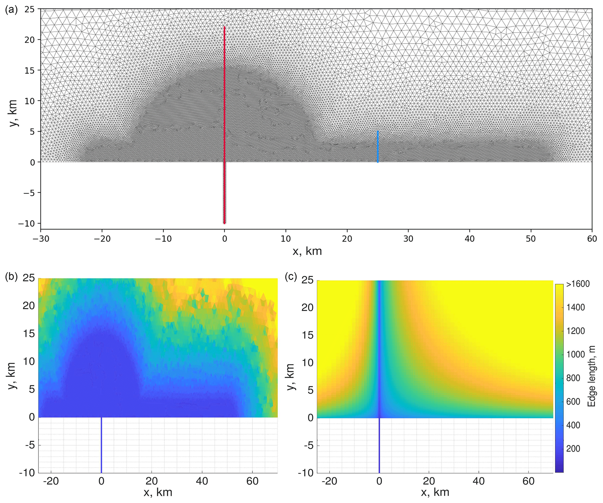
Figure 2 (a) The triangular mesh with a refinement in the plume spreading area; the lines indicate cross-sectional positions. (b, c) Edge length of the triangular and quadrilateral meshes (m) with a zoomed-in view of the plume spreading area.

We performed the simulations on triangular and quadrilateral meshes with variable resolution. The quadrilateral mesh is a bit coarser in the plume spreading area (Fig. 2). The triangular mesh consists of 76 524 triangles and 37 900 vertices. The quadrilateral mesh consists of 59 706 vertices and 59 122 cells.

The 3D reference grid has $k_{max}=\mathrm{40}$ sigma layers zoomed parabolically towards the surface at σ(0):

$$\begin{array}{}\text{(2)}& \mid \mathit{\sigma }\left(k\right)\mid ={\left({\displaystyle \frac{k}{k_{max}}}\right)}^{\mathrm{2}},\text{for }k=\mathrm{0},\mathrm{\dots },k_{max}.\end{array}$$

Note that the sign of the sigma depends on the code realization and how the z axis is directed.

Table 1 The description of the setups. Bold font in the inner part of the table indicates the changes compared to the default run. The discharge in all setups was equal to 3000 m³ s⁻¹.

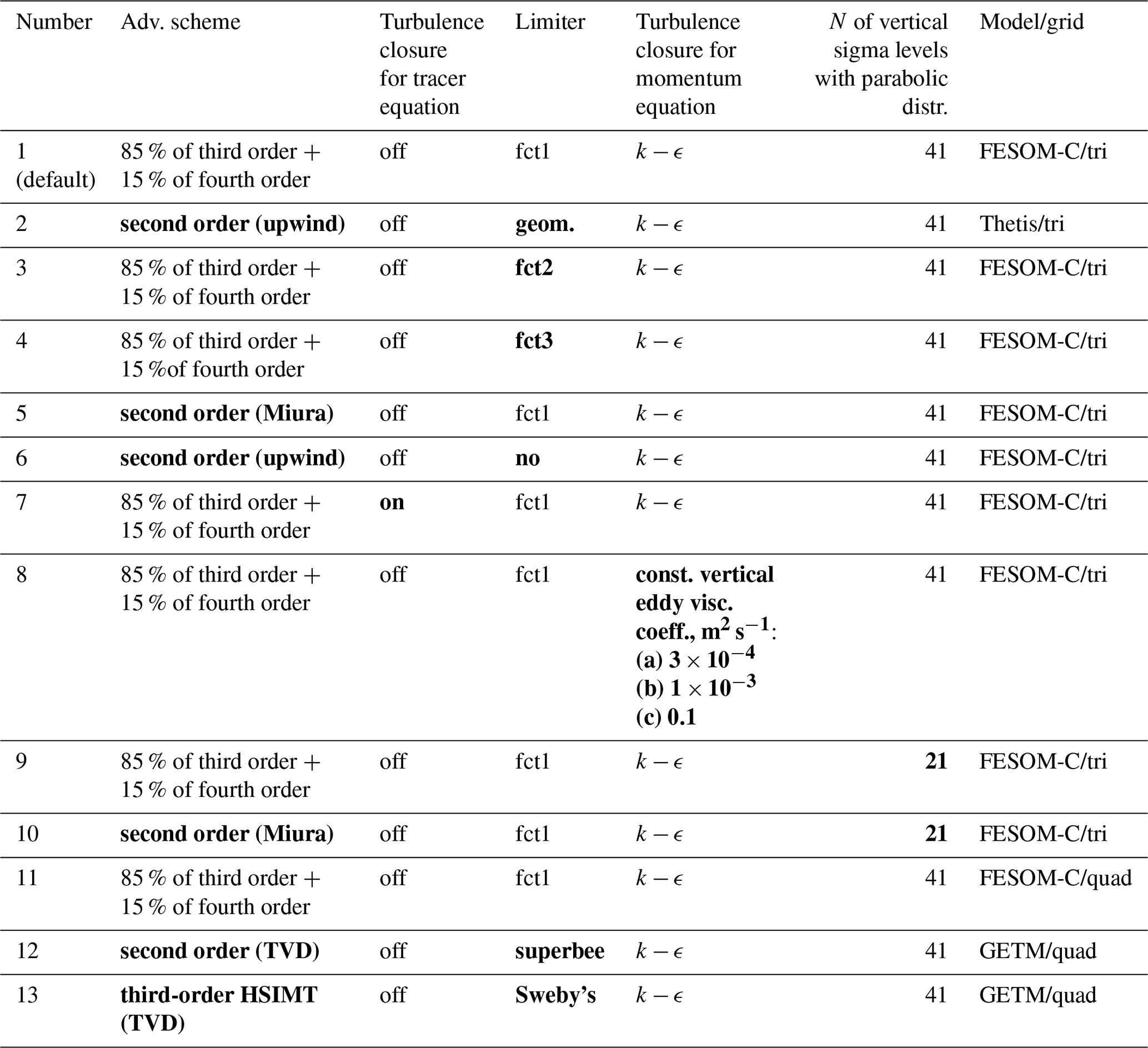
Since our main intention is to learn about the effect of hidden mixing, the experiments mostly differ by the advection schemes and limiters used. Their description is presented in Table 1. The models, advection schemes, and limiters are described below in Sect. 2.3.

Discussion of the viscosity effect is largely based on the additional set of simulations with a constant vertical eddy viscosity coefficient equal to $\mathrm{2.5}\times {\mathrm{10}}^{-\mathrm{4}}$ m² s⁻¹ and increased discharge equal to 3900 m³ s⁻¹ (Table A1). (These simulations are not considered in Sect. 5, but only in Sect. 6.)

2.3 Circulation models

2.3.1 FESOM-C

FESOM-C is a coastal branch of the global Finite volumE Sea ice Ocean Model (FESOM2) (Danilov et al., 2017; Androsov et al., 2019; Fofonova et al., 2019; Kuznetsov et al., 2020). FESOM-C solves 3D primitive equations in the Boussinesq, hydrostatic, and traditional approximations for the momentum, continuity, and density constituents, and it uses a terrain-following coordinate in the vertical. It has the cell vertex finite-volume discretization (quasi-B-grid) and works on any configurations of triangular, quadrangular, or hybrid meshes (Danilov and Androsov, 2015; Androsov et al., 2019). The schemes to compute vertical eddy viscosity and diffusivity can be chosen via the coupled General Ocean Turbulence Model (Burchard et al., 1999).

The numerical scheme of FESOM-C splits the fast and slow motions into barotropic and baroclinic subsystems (Lazure and Dumas, 2008). It uses an asynchronous time stepping, assuming that integration of temperature and salinity is half-step-shifted with respect to momentum.

Three schemes have been implemented in FESOM-C for horizontal advection (Androsov et al., 2019): upwind, Miura (Miura, 2007), and MUSCL-type (van Leer, 1979). The first two are based on linear reconstruction and are second-order in space and time. The linear reconstruction upwind scheme and the Miura scheme differ in the implementation of time stepping. The first needs the Adams–Bashforth method to be second-order with respect to time. The scheme by Miura achieves this by approximately tracking the volumes advected through the faces of control volumes.

The third approach used in the model is based on the gradient reconstruction (MUSCL-type scheme). The idea of this approach is to estimate the tracer at control volume faces by a linear reconstruction using the combination of centered and upwind gradients. It represents a combination of the third-order and fourth-order fluxes in space in a fraction of 85 % and 15 %, respectively. The method is second-order accurate in time.

The upwind advection scheme is used together with a third-order scheme in the vertical; the Miura and MUSCL-type schemes use a fourth-order vertical advection.

In all cases, momentum advection is treated with a second-order upwind scheme.

In this paper, the tracer advection schemes are run in combination with the FCT (flux-corrected transport) algorithm. We use three options to constrain the anti-diffusive flux, which is added to the solution obtained with the positivity-preserving low-order scheme. In the fct1 option the admissible increments for each scalar point are sought over its horizontal neighbors and in the clusters above and below them, which leaves wide bounds because vertical gradients are typically larger. The fct2 option is similar to the fct1 except for the search of vertical bounds, which is done locally (tracer values above and below). In the fct3 option the vertical bounds are taken into account only if they are narrower than the horizontal ones. In all options the admissible increments are computed with respect to the combination of the low-order solution and the solution at the previous time step.

2.3.2 Thetis

Thetis is a 3D hydrostatic circulation model based on discontinuous Galerkin (DG) finite-element formulation (Kärnä et al., 2018; Kärnä, 2020). Thetis uses an unstructured triangular or quad mesh in the horizontal direction and an extruded prismatic 3D mesh. All prognostic variables are discretized with linear discontinuous elements ($P_{\mathrm{1}}^{\text{DG}}$); in 3D the elements are $P_{\mathrm{1}}^{\text{DG}}$ in both the horizontal and vertical direction. A second-order strong stability-preserving (SSP) Runge–Kutta time integrator is used to march the equations in time. The 3D dynamics are treated explicitly except vertical diffusion, which is treated implicitly; a split-implicit mode-splitting technique is used to solve the free surface dynamics. The 3D mesh tracks the position of the free surface. Tracer advection is implemented with upwind fluxes at element interfaces. In addition, a geometric slope limiter (Kuzmin, 2010) is employed as a post-process step to suppress overshoots: if the tracer value at a node exceeds the maximum mean value of the neighboring elements, it is marked as an overshoot. The tracer is then redistributed in the element until none of the nodes violate the extrema conditions or the element is fully mixed (i.e., all nodes have the same value). The geometric limiters and the SSP time integration method guarantees that the advection scheme is positive definite; i.e., no spurious overshoots are generated. The same advection scheme is applied to both tracers and momentum. The discretization of the Thetis dynamical core is described in Kärnä et al. (2018).

The Thetis solver is formally second-order in space and time with the exception of vertical diffusion (first-order in time) and areas where the slope limiter is active (reducing the scheme to first-order). The slope limiters do impose some numerical diffusion on the solution, even in the case that tracer diffusion operators are omitted.

2.3.3 GETM

GETM is an open-source coastal ocean model (http://www.getm.eu, last access: 12 November 2021; Burchard and Bolding, 2002). It solves the Reynolds-averaged Navier–Stokes equations under the Boussinesq approximation together with transport equations for temperature and salinity on a C-staggered structured finite-volume grid. For the present study the non-hydrostatic option by Klingbeil and Burchard (2013) and the temperature equation are not activated. The numerics of GETM are similar to other coastal ocean models (Klingbeil et al., 2018). The free surface is integrated in a split-explicit mode-splitting procedure. For the present study the 3D time step of 60 s is split into 24 subcycles. In the vertical GETM supports adaptive terrain-following coordinates (Hofmeister et al., 2010; Gräwe et al., 2015), but for the present study fixed sigma coordinates according to Eq. (2) are used. Advection of momentum and tracers is carried out by directional splitting with TVD (total variation diminishing) schemes. In the current study the same scheme was used for the advection of both momentum and the tracer. In order to induce minimum numerical mixing (Klingbeil et al., 2014), in the present study the superbee limiter is applied, which is known by its anti-diffusive (anti-viscous) character, in combination with the second-order advection scheme (spatially and temporally). Additionally, the HSIMT third-order TVD scheme (second-order temporally) equipped with Sweby's limiter is applied (Wu and Zhu, 2010). If necessary, in individual water columns the vertical advection is automatically iterated to comply with the CFL (Courant–Friedrichs–Lewy) condition in very thin cells. The turbulent vertical viscosity is calculated by the turbulence module of GOTM (Burchard et al., 1999) in terms of stratification and shear provided by GETM.

3 Analytical prediction for the plume behavior

In this section we summarize the qualitative and quantitative predictions of the plume behavior in the absence of diffusive processes and when they are present in the system (see the respective notes at the end of the subsections) during the first two inertial periods.

3.1 Mouth area and near-field zone

The mouth area represents a control section for classical hydraulic channel flow (Gill, 1977). The narrow mouth causes rapid shoaling and seaward expansion of the pycnocline, as well as an acceleration of the upper fresh layer with a significant Froude number gradient, reaching supercritical conditions as fresh water comes out of the river channel. In effect this means that the entire disturbance is swept downstream. Shear increases at the base of an accelerating plume, resulting in very pronounced viscous effects. The presence of supercritical conditions causes a nearly fully inertial momentum balance (Garvine, 1987). The acceleration of the plume in the near-mouth area leads to a drop in surface pressure following the Bernoulli principle such that we expect a local drop in sea surface height relative to the channel (e.g., Hetland, 2010). In the limit of zero eddy diffusivity in the tracer equation, for the narrow river mouth and large discharge, the water exchange between the river channel and the shelf is very limited due to constraints imposed by hydraulic control, river momentum (e.g., Gill, 1977; Stommel and Farmer, 1953; Farmer and Armi, 1986; Hetland, 2010; Armi and Farmer, 1986), and the Knudsen (1900) relation.

The experiments with larger discharge – 3900 m³ s⁻¹ – suppose that the interface in the mouth area between layers of different densities should reach the bottom (the fresh water should extend all the way to the bottom) given the absence of bottom friction and presence of relatively large river velocities (which are larger than the frontier velocities in the lock-exchange experiment corresponding to the given pressure gradient). According to Armi and Farmer (1986) we have a case of intermediate barotropic flow (induced by river momentum) when the dense water stays motionless and does not penetrate through the constriction (in our case it is the mouth). Thus, we are expecting the area where the freshwater flow loses contact with the bottom and a plume actually forms to be situated directly in the mouth area (e.g., MacDonald and Geyer, 2005).

The experiments with a smaller discharge – 3000 m³ s⁻¹ – suppose penetration of the dense water into the river channel only in the case when the large viscous effect initiated by the hydraulic jump is neglected at least partly (e.g., by prescribed upper bounds for the eddy vertical viscosity or only background viscosity in numerical solutions). In the inviscid theory of Armi and Farmer (1986) the barotropic force initiated by the river momentum in this case can be characterized as a transition between moderate to intermediate flow conditions, and penetration of the dense water into the river channel can take place. The viscous effects naturally block the dense water penetration into the river channel; however, numerical mixing may provoke it. Even in the absence of explicit diffusion operators there is some mixing in numerical simulations. Numerical mixing is largely attributed to the advection scheme and the limiters built into it. It can lead to dense water penetration into the river channel and the appearance of new salinity classes in the river channel. For any tracer c, the total (advective plus diffusive) tracer flux per unit area of a transect or isohaline can be defined as $F^c=u_{\mathrm{n}}c-K_{\mathrm{n}}{\partial }_{\mathrm{n}}c$, where u_n is the outgoing normal velocity, ∂_nc is the tracer gradient normal to the surface, and K_n is diffusivity in the direction normal to the surface. Let us take the mouth transect directly upstream from supercritical conditions. It is clear that the presence of a large enough numerical mixing can provoke dense water penetration into the river channel. The density intrusion in this case will have a hydraulically controlled, blunt-faced profile (e.g., Jirka and Arita, 1987). If we apply the equation written above to the isohaline of the freshwater layer and activate vertical eddy diffusivity, we will also get dense water penetrating into the system, with the hydraulic control setting the upper limit of exchange as well as a more complex interface (e.g., MacCready and Geyer, 2001). We will return to this topic in the Discussion section.

3.2 Bulge

Here we revisit the definition of a bulge according to the review by Horner-Devine et al. (2015) as a continuation of the near-field zone in which Earth’s rotation in the momentum balance begins to predominate, turning the plume to the right (in the Northern Hemisphere) and creating a gyre in thermal wind balance. Note that the near-field zone, bulge, and coastal current have a very complex dynamic structure such that the consideration of various discharge characteristics is needed to clearly describe it. We prefer to avoid this by focusing on the resulting plume spreading characteristics: maximum offshore plume spreading position, internal bulge radius (nearshore radius), and the alongshore bulge length. Avicola and Huq (2003) showed that on average the bulge alongshore spread is longer than its offshore spread and that this ellipticity is constant through time and equal to ∼1.3. Thus, it suffices for us to locate the maximum of bulge offshore spreading and let the alongshore scale be a control point.

We know that when the channel is at a right angle to the coast the bulge grows continuously over time because its increasing size creates a balance between the momentum flux associated with the downstream current and the compensating Coriolis force associated with the migration of the gyre center away from the coast (e.g., Fong et al., 1997; Nof and Pichevin, 2001; Horner-Devine et al., 2006, 2009). But the expansion of the bulge leads to radial and advective acceleration terms that are 2 orders of magnitude smaller than the terms of the gradient–wind balance. Accordingly, the gradient–wind balance is expected to apply even for a growing bulge as long as its radius is sufficiently large (Horner-Devine et al., 2006, 2009). Recent studies have shown that the bulge offshore radius and displacement of bulge center from the wall (nearshore radius) can be respectively scaled with the internal Rossby radius (L₀) and inertial radius (L_b), both of which are constant over time (Horner-Devine et al., 2009). In our case $L^{\ast }=\frac{L_{\mathrm{0}}}{L_{\mathrm{b}}}\approx \mathrm{1}$, so the river flow is one of the main factors pushing the bulge offshore (the anticyclonic circulation is nearly offshore radii), and the bulge is prone to instability (Horner-Devine et al., 2009). Thus, the net shore-directed Coriolis force is small, the angle of incidence of the recirculating bulge flow that it makes with the coast is greater than 90^∘ (flow directed back upstream) (Whitehead, 1985; Horner-Devine et al., 2009), and the majority of the impinging fluid is directed back into the bulge. This feature largely makes the bulge size sensitive to any source of mixing in the model. The laboratory and theoretical studies mentioned above have found that the plume starts turning to the right in the Northern Hemisphere at approximately one-fourth of the inertial period at a radius of about L₀ and reaches thermal wind balance after one to two rotation periods.

To obtain an estimate for the offshore spreading of the bulge in the absence of diffusive processes, we revisit the equations provided by Yankovsky and Chapman (1997) and propose some modifications. We consider flow in the bulge to be in cyclostrophic balance as described by the following momentum equation:

$$\begin{array}{}\text{(3)}& -{\displaystyle \frac{u_{\mathrm{c}}^{\mathrm{2}}}{r}}-f{u}_{\mathrm{c}}=-g^{\prime }{\displaystyle \frac{\partial h_{\mathrm{b}}}{\partial r}},\end{array}$$

where u_c is the azimuthal cyclostrophic velocity at the radial distance r from the anticyclone center, and h_b is the thickness of the buoyant layer.

Because of a purely surface-advected plume at the shelf, we assume no interaction of the plume with the bottom and a plume thickness of h_b, which changes little from the mouth area to the center of the anticyclonic bulge and gradually decreases to zero along the outer edge. This means that $\frac{\partial h_{\mathrm{b}}}{\partial r}$ is equal to zero along the streamline from the mouth to the anticyclonic center, and it can be expressed as $\frac{-h_{\mathrm{c}}}{r}$ from the bulge center to its offshore edge, where h_c is the depth of the bulge center and r is the offshore radius of the bulge. Returning to Eq. (3) we get

$$\begin{array}{}\text{(4)}& r={\displaystyle \frac{-\left(g^{\prime }{h}_{\mathrm{c}}+{u_{\mathrm{c}}}^{\mathrm{2}}\right)}{f{u}_{\mathrm{c}}}}.\end{array}$$

To get u_c, the Bernoulli function for the buoyant layer (Gill, 1982) can be applied:

$$\begin{array}{}\text{(5)}& B=g^{\prime }{h}_{\mathrm{b}}+{\displaystyle \frac{u_{\mathrm{b}}^{\mathrm{2}}}{\mathrm{2}}},\end{array}$$

where u_b is the averaged velocity of the layer occupied by the plume. In the absence of diffusion B should be constant along the streamline. In Yankovsky and Chapman (1997), inflow is connected to the outer edge and h_c=h₀ (h₀ is the inflow depth). This poses two major problems: (i) h₀ and h_c can be significantly different in a purely surface-advected plume, as (in our case) a lift-off point is situated immediately at the mouth or even upstream and is accomplished by the hydraulic jump in the mouth; and (ii) the bulge continuously grows over time.

As mentioned above, the gradient–wind balance is expected to apply even to a growing bulge as long as its radius is sufficiently large (Horner-Devine et al., 2006, 2009). So (ii) can be addressed as follows: we determine the radius of the bulge when the plume forms even though at that point the coastal current is already in place and the bulge is in thermal wind balance. Our particular test case places no focus on a slow mode of bulge growth (as covered in Nof and Pichevin, 2001); our task is rather to obtain a short-term prediction once the bulge has reached thermal wind balance. Point (i) can be addressed by introducing the so-called geostrophic depth, h_g, or the depth of the plume in the near-field zone within critical conditions and taking into account the fact that the diffusive processes are absent in our consideration. It is well known that the inflow momentum is the most important factor defining the position of the bulge center (e.g., Horner-Devine et al., 2006) and that the depth of the bulge center becomes proportional to the geostrophic depth as soon as the bulge attains thermal wind balance (e.g., Avicola and Huq, 2003; Yankovsky and Chapman, 1997). The equation for h_g above is based on consideration of a two-layer Margules front system that has a quiescent lower layer and an upper layer in thermal wind balance or in geostrophic cross-shore momentum balance (valid for a coastal current; see below) with uniform vertical shear of the alongshore plume velocity. Then we assume that the entire buoyancy inflow transport (=Q_r) accumulates in the frontal zone (e.g., Yankovsky and Chapman, 1997; Fong and Geyer, 2002). Finally, we get

$$\begin{array}{}\text{(6)}& h_{\mathrm{c}}=h_{\mathrm{g}}=\sqrt{{\displaystyle \frac{\mathrm{2}W{u}_{\mathrm{0}}{h}_{\mathrm{0}}f}{g^{\prime }}}}=\mathrm{1.8}\left(\mathrm{2}\right)\mathrm{m}.\end{array}$$

So, we can determine the properties of the bulge when the bulge center is located at this level. Naturally, it takes place only at the beginning of the plume evolution. The bulge continuously grows not only offshore, but also in depth; however, this is at a slower rate. The whole discharge accumulates in the bulge only for a very short period of time prior to the appearance of the coastal current. The front expands at approximately the surface gravity wave speed within the layer h_g, so we connect the outer edge to the following flow conditions.

$$\begin{array}{}\text{(7)}& {\displaystyle \frac{\mathrm{3}}{\mathrm{2}}}{g}^{\prime }{h}_{\mathrm{g}}={\displaystyle \frac{\mathrm{3}}{\sqrt{\mathrm{2}}}}\sqrt{W{u}_{\mathrm{0}}{h}_{\mathrm{0}}f{g}^{\prime }}={\displaystyle \frac{u_{\mathrm{c}}^{\mathrm{2}}}{\mathrm{2}}}\text{(8)}& {\displaystyle }\begin{array}{rl}{u}_{\mathrm{c}}& =-\sqrt[\mathrm{4}]{\mathrm{18}W{u}_{\mathrm{0}}{h}_{\mathrm{0}}f{g}^{\prime }}=-\sqrt[\mathrm{4}]{\mathrm{18}{Q}_{\mathrm{r}}f{g}^{\prime }}\\ & \approx -\mathrm{1.1}\left(\mathrm{1.17}\right)\mathrm{m}{\mathrm{s}}^{-\mathrm{1}}\end{array}\text{(9)}& {\displaystyle }r={\displaystyle \frac{\mathrm{4}}{\sqrt{\mathrm{3}}}}{\displaystyle \frac{\sqrt{g^{\prime }{h}_{\mathrm{g}}}}{f}}\approx \mathrm{12.2}\left(\mathrm{12.9}\right)\mathrm{km}\end{array}$$

This radius r in Eq. (9) represents an offshore radius of the bulge in our test case as soon as the gyre is in thermal wind balance and its center is about h_g thick. Based on the L^∗ value calculated above, the nearshore radius should be close to the offshore radius. This can be expected after one to two rotational periods based on laboratory experiments and simple calculations from the internal Rossby radius, h_g or h_c, and associated surface gravity wave speed (e.g., Hetland and MacDonald, 2008; Wright and Coleman, 1971; Hetland, 2010). The predicted radius is consistent with laboratory experiments published by Avicola and Huq (2003) and Horner-Devine et al. (2006) after approximately one to two rotational periods as soon as the gyre is in thermal wind balance. However, these experiments predict for such a radius (relatively to the Rossby radius) at least 1.5 times (Horner-Devine et al., 2006) or even twice (Avicola and Huq, 2003) as much deepening at the center. Horner-Devine et al. (2006) related their findings of a smaller central depth to different measurement techniques. Defining the bulge depth based on reference buoyancy (20 % of the inflow buoyancy) instead of the maximum vertical gradient, one obtains greater deepening. Deepening of the gyre center is a relatively slow process and is usually quasi-stationary after several rotational periods. Deepening at the center is largely attributed to mixing and dilution processes at the plume base, and the analytical solution does not consider the influence of diffusive processes. In our simulations we omit the physical diffusivity (eddy diffusivity is set to zero in the tracer equation) in order to reproduce the analytical estimations about the bulge offshore spreading. As for the position of the bulge center relative to the x axis, recirculation of the discharged water can take place only to the right of the river mouth. On the other hand, we have defined the bulge in such a way that a part of it is found to the left of the source. Baroclinic instability can also lead to rotated structures in the area of interest due to relatively fast radial (compared to vertical) bulge growth (e.g., Avicola and Huq, 2003). We are therefore not going to find the exact bulge center position by defining it only on the x axis as the site of maximum offshore spreading of the bulge.

Note that in our idealized conditions the bulge becomes nearly symmetrical and tends toward instability, which suggests a solution sensitive to mixing. Any additional diffusion in the bulge zone and/or near-field zone will directly reduce the bulge external radius, displace its center, and change the angle at which the bulge characteristics impinge upon the coastal zone. A small isohaline area requires greater mixing than a large one to maintain the same freshwater discharge across the isohaline (Hetland, 2005; Burchard, 2020). So either the bulge tends to be less restricted offshore and in parallel deeper, and/or the bulge tends to be less restricted offshore together with a reduced discharge rate associated with the bulge (the bulge will be sliced off and the impingement angle will be changed).

3.3 Coastal current

In this subsection we are going to derive the coastal current characteristics, in particular the bounds for the coastal current depth near the wall, the bounds for the near-wall speed, and the coastal current offshore spread. Typically, the coastal current has a quasi-triangular profile in the offshore cross section, so when we are talking about near-wall depth and speed we mean maximum depth and speed at each offshore cross section. Below we will omit “near the wall” for simplicity.

We can calculate the discharge attributed to the coastal current, Q_cc, based on the current bulge vorticity (e.g., Nof and Pichevin, 2001).

$$\begin{array}{}\text{(10)}& {\displaystyle }\mathit{\alpha }={\displaystyle \frac{-\mathrm{2}{u}_{\mathrm{c}}}{f\cdot r}}\approx \mathrm{1.5}\left(\mathrm{1.51}\right)\text{(11)}& {\displaystyle \frac{Q_{\mathrm{cc}}}{Q_{\mathrm{r}}}}={\displaystyle \frac{\mathrm{1}}{\mathrm{1}+\mathrm{2}\mathit{\alpha }}}\approx \mathrm{0.25}\left(\mathrm{0.248}\right)\end{array}$$

Based on the obtained Q_cc , we arrive at a minimum freshwater layer thickness to be expected for the coastal current.

$$\begin{array}{}\text{(12)}& h_{min}=\sqrt{{\displaystyle \frac{\mathrm{2}{Q}_{\mathrm{cc}}f}{g^{\prime }}}}\approx \mathrm{0.9}\left(\mathrm{1}\right)\mathrm{m}\end{array}$$

Naturally, the geostrophic depth h_g calculated above gives us the maximum freshwater layer thickness, h_max, to be expected in the coastal current if the total discharge from the river goes to the coastal current for some reason. We already know that in our case a large portion of the fresh water stays in the bulge. However, when L^∗ is large, the bulge may be unstable, separating from and re-attaching to the wall and causing a pulsed flow of the coastal current (Horner-Devine et al., 2006). Furthermore, when the coastal current forms, a different portion of the fresh water may go with it depending on the time moment. The geostrophic depth therefore provides a good estimate of the maximum depth of the layer influenced by the coastal current.

The coastal current propagates at a speed given by $c_{\mathrm{n}}=\sqrt{g^{\prime }\cdot h}$, and the propagation speed should therefore be between 0.45 (0.47) and 0.64 (0.67) m s⁻¹ taking into consideration h_min and h_max, respectively. Based on these values we derive a local Rossby radius equal to 3.75 (3.9)–5.3 (5.6) km. We can expect the coastal current to occupy this width in the nose zone at the beginning of the plume history. Predicting the width of the coastal current in the upstream area between the source and the nose is not a trivial task (a problem already identified by Garvine, 1995). However, it is clear that the position of the bulge center should largely determine the coastal current maximum offshore width in the considered time frame. We already know that a nearshore radius of the bulge is about 12 km after one to two rotational periods, which is at about two internal Rossby radii. This result is in agreement with laboratory experiments (Avicola and Huq, 2003; Horner-Devine et al., 2006) wherein the width may be up to two local Rossby radii after one to two rotational periods. To summarize, we can provide a relatively wide window for the expected coastal current offshore width; it can vary between 12 km near the source zone for both runs and 3.75 km (3.9 km) in the nose zone.

Note that in the presence of nonzero eddy diffusivity, we can expect a larger amount of the discharge to enter the coastal current because the bulge in the non-diffusive case is nearly symmetrical (in the sense of internal – near coast – and offshore radii) and reaches maximum offshore extension. Therefore, in principle, the coastal current discharge could be used as an indicator for numerical diffusivity. Such an approach is not used here, as it would require considering many rotational periods for a precise estimation.

4 Diagnostic of the numerical diffusivity

The coastal current discharge rate and offshore spread as well as asymmetry or the characteristic impingement angle of the bulge can all be considered indirect measures of numerical mixing. However, each of these measures requires additional analysis and has some limitations.

We base our analysis on isohalines and salinity classes following the work by Hetland (2005), Wang et al. (2017), and Burchard (2020). Using the balance equation for salinity and the mass conservation law we obtain a budget equation for the salt content integrated over all salinities between the river salinity S_r and the salinity of the isohaline, S:

$$\begin{array}{}\text{(13)}& {\displaystyle \frac{\partial }{\partial t}}\underset{S_{\mathrm{r}}\mathit{⩽}s\mathit{⩽}S}{\iiint }\left(S-s\right)\mathrm{d}V=\left(S-S_{\mathrm{r}}\right)\cdot Q_{\mathrm{r}}+\underset{s=S}{\iint }{\mathit{f}}_{\mathrm{diff}}\cdot \mathit{n}\mathrm{d}\mathit{\sigma },\end{array}$$

where f_diff is the diffusive salinity flux vector, and n is the outward normal unit vector, both located on the isohaline S. Neglecting physical diffusion and assuming zero river salinity (S_r=0), the diahaline flux is related to numerical mixing so that the numerically induced salinity discharge (total salinity transport) through the isohalines S can be calculated as

$$\begin{array}{}\text{(14)}& \begin{array}{rl}{F}^s\left(S\right)& =\underset{s=S}{\iint }{\mathit{f}}_{\mathrm{num}}\cdot \mathit{n}\mathrm{d}\mathit{\sigma }\\ & ={\displaystyle \frac{\partial }{\partial t}}\left(\underset{\mathrm{0}\mathit{⩽}s\mathit{⩽}S}{\iiint }\left(S-s\right)\mathrm{d}V\right)-S\cdot Q_{\mathrm{r}}.\end{array}\end{array}$$

Note that numerical mixing may also include anti-diffusive effects. For further analysis, we divide Eq. (14) by S, which gives the diahaline diffusive freshwater discharge or total freshwater transport across the isohaline (related to numerical mixing):

$$\begin{array}{}\text{(15)}& F\left(S\right)={\displaystyle \frac{F^s\left(S\right)}{S}}.\end{array}$$

By dividing the discharges F^s(S) and F(S) by the isohaline area, A(S), the respective average diahaline fluxes and transport are obtained:

$$\begin{array}{}\text{(16)}& f^s\left(S\right)={\displaystyle \frac{F^s\left(S\right)}{A\left(S\right)}},f\left(S\right)={\displaystyle \frac{F\left(S\right)}{A\left(S\right)}}.\end{array}$$

We further define the diahaline velocity as

$$\begin{array}{}\text{(17)}& w^{\mathrm{dia}}\left(S\right)={\displaystyle \frac{\partial f^s\left(S\right)}{\partial S}}\end{array}$$

and note that only under stationary conditions with $F^s\left(S\right)=-S{Q}_{\mathrm{r}}$ are both w^dia(S) and f(S) identical.

For the analysis of the different models results, we will be using time-averaged transports and fluxes:

$$\begin{array}{}\text{(18)}& \begin{array}{rl}& {\stackrel{\mathrm{‾}}{F}}^s\left(S\right)=\langle F^s\left(S\right)\rangle ,\stackrel{\mathrm{‾}}{F}\left(S\right)=\langle F\left(S\right)\rangle ,\\ & {\stackrel{\mathrm{‾}}{f}}^s\left(S\right)={\displaystyle \frac{\langle F^s\left(S\right)\rangle }{\langle A\left(S\right)\rangle }},\stackrel{\mathrm{‾}}{f}\left(S\right)={\displaystyle \frac{\langle F\left(S\right)\rangle }{\langle A\left(S\right)\rangle }},\\ & {\stackrel{\mathrm{‾}}{w}}^{\mathrm{dia}}\left(S\right)={\displaystyle \frac{\partial {\stackrel{\mathrm{‾}}{f}}^s\left(S\right)}{\partial S}},\end{array}\end{array}$$

where 〈⋅〉 denotes a time average.

For the diagnostics of numerical mixing presented above the salinity range is divided into isohaline classes, and the volume of each class is calculated. These volumes are useful diagnostics as soon as numerical mixing creates the volumes between the first and last salinity classes.

5 Results

In describing the results, we focus primarily on the first two simulations from Table 1. The differences in the dynamics of these runs facilitate the interpretation of other runs. Additional simulations (see Table 1) have been conducted to illustrate the plume dynamics’ sensitivity to certain parameters. Runs 11, 12, and 13 are performed on a quadrilateral mesh with FESOM-C and GETM; their performance is described at the end of this section. When comparing runs 11, 12, and 13 with the others, one should keep in mind that the resolutions of the rectangular and triangular grids are not identical (Fig. 2). The results of these runs are therefore presented separately despite the fact that they are discussed in the same frame.

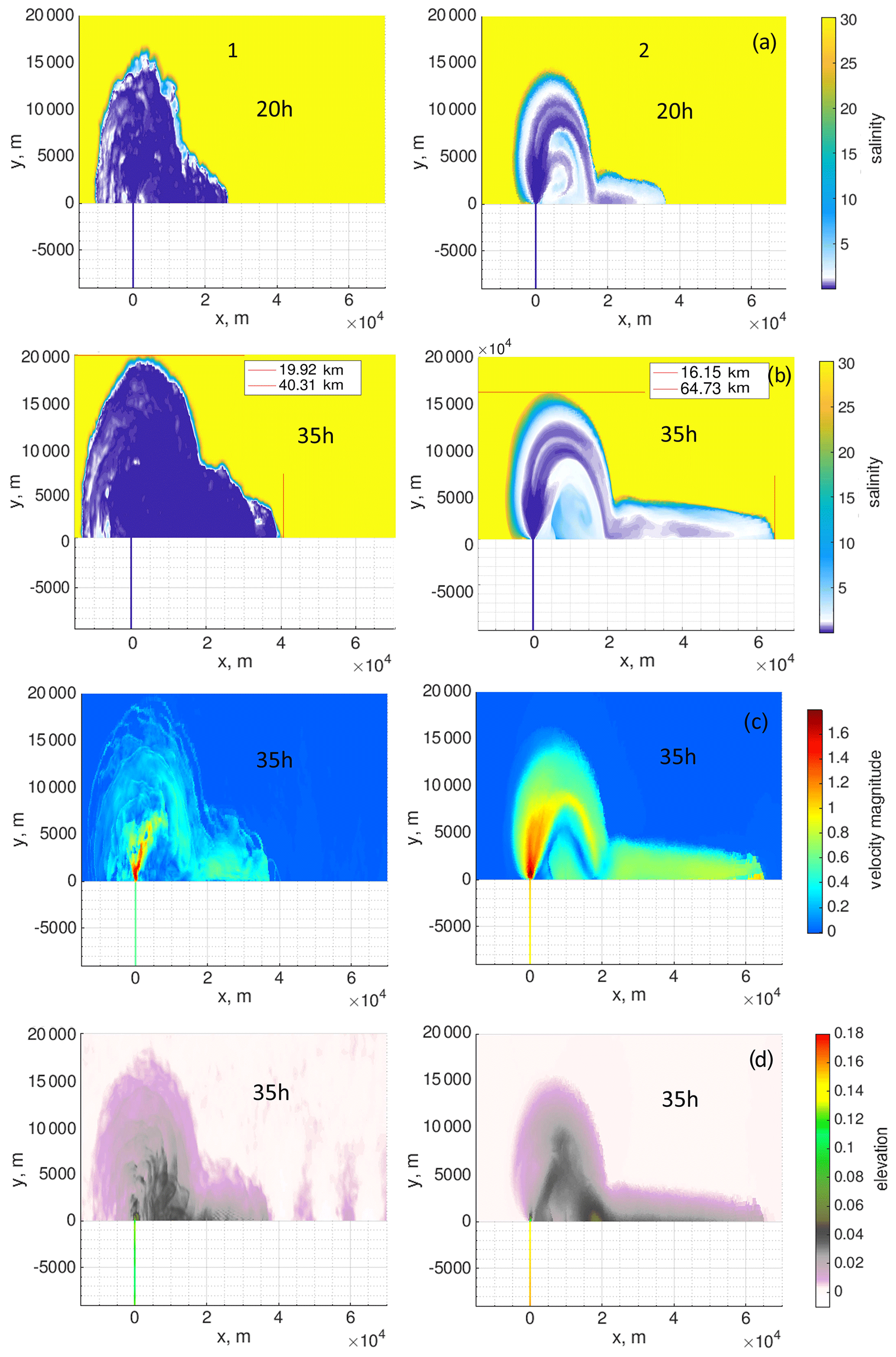
Figure 3 Results of runs 1 (left panels) and 2 (right panels) after 20 and 35 h: (a) surface salinity, in practical scale, at 20 h; (b) surface salinity, in practical scale, at 35 h; (c) surface velocity (m s⁻¹) at 35 h; (d) surface elevation (m) at 35 h.

Table 2 Summary of the results after 20 and 35 h of runs 1 and 2. The mean value of the coastal current discharge at different time moments should be compared with the analytical solution. Numbers in bold font demonstrate the bulge offshore spread (width) based on simulated length divided by 1.3; 1.3 is the ratio between the length and width obtained in a laboratory study.

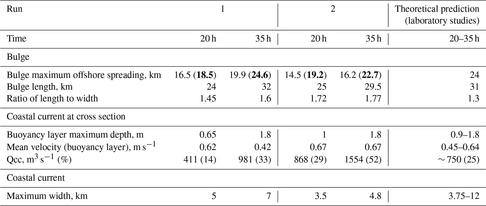
Figure 3 and Table 2 contains information about the predicted characteristics of the plume's behavior. To summarize, we would expect the bulge's offshore spread to extend for no less than 24 km after two inertial periods accumulating about 75 % of the total freshwater runoff. We would expect its surface to be fresh, with the coastal current transporting only about 25 % of the total freshwater runoff. We stress that these characteristics are not independent, of course, and that if the surface of the plume is fresh, the offshore spread of the bulge can generally be treated as a final indicator of the model's performance.

Figure 3 compares the surface salinity, velocity, and elevation for runs 1 and 2 after one and two inertial periods, i.e., after 20 and 35 h. This figure illustrates that in both simulations, the plume starts turning right after one-quarter of the rotational period at a distance of one inertial radius (∼5 km). In both simulations, the coastal current begins to form after one rotational period. But the differences between the way each simulation represents the bulge and the coastal current dynamics are nevertheless substantial, even after one and especially after two inertial periods. The main differences between the two runs are summarized in Table 2.

5.1 Mouth area and near-field zone

In agreement with observational studies (e.g., Wright and Coleman, 1971; MacDonald and Geyer, 2004), river water leaves the narrow estuary and rapidly shoals over a distance of a few channel widths in both runs. The velocities in the shoaling zone reach initial surface gravity wave speeds of ∼1.5 m s⁻¹ or more, which is as expected (e.g., Hetland and MacDonald, 2008; Wright and Coleman, 1971; Hetland, 2010). In both runs, the near-field area is also characterized by supercritical conditions and a hydraulic jump (see Figs. 4 and 6).

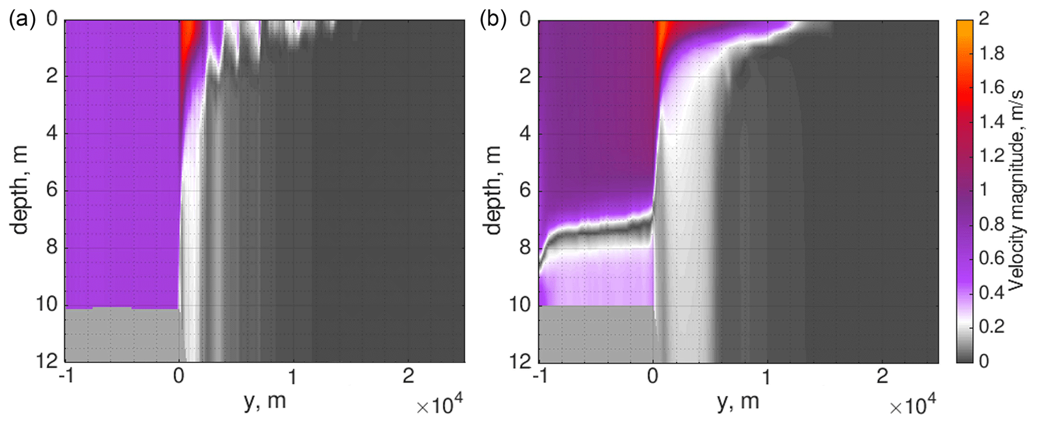
Figure 4 The magnitude of the velocity at the mouth cross section based on runs 1 (a) and 2 (b) at the 20 h time moment.

Figure 5 The surface salinity (left panels) and salinity at the mouth cross section (right panels), in practical scale, at 35 h in different runs indicated by the number (see Table 1). The bulge offshore spreading and the coastal current propagation are shown by red lines.

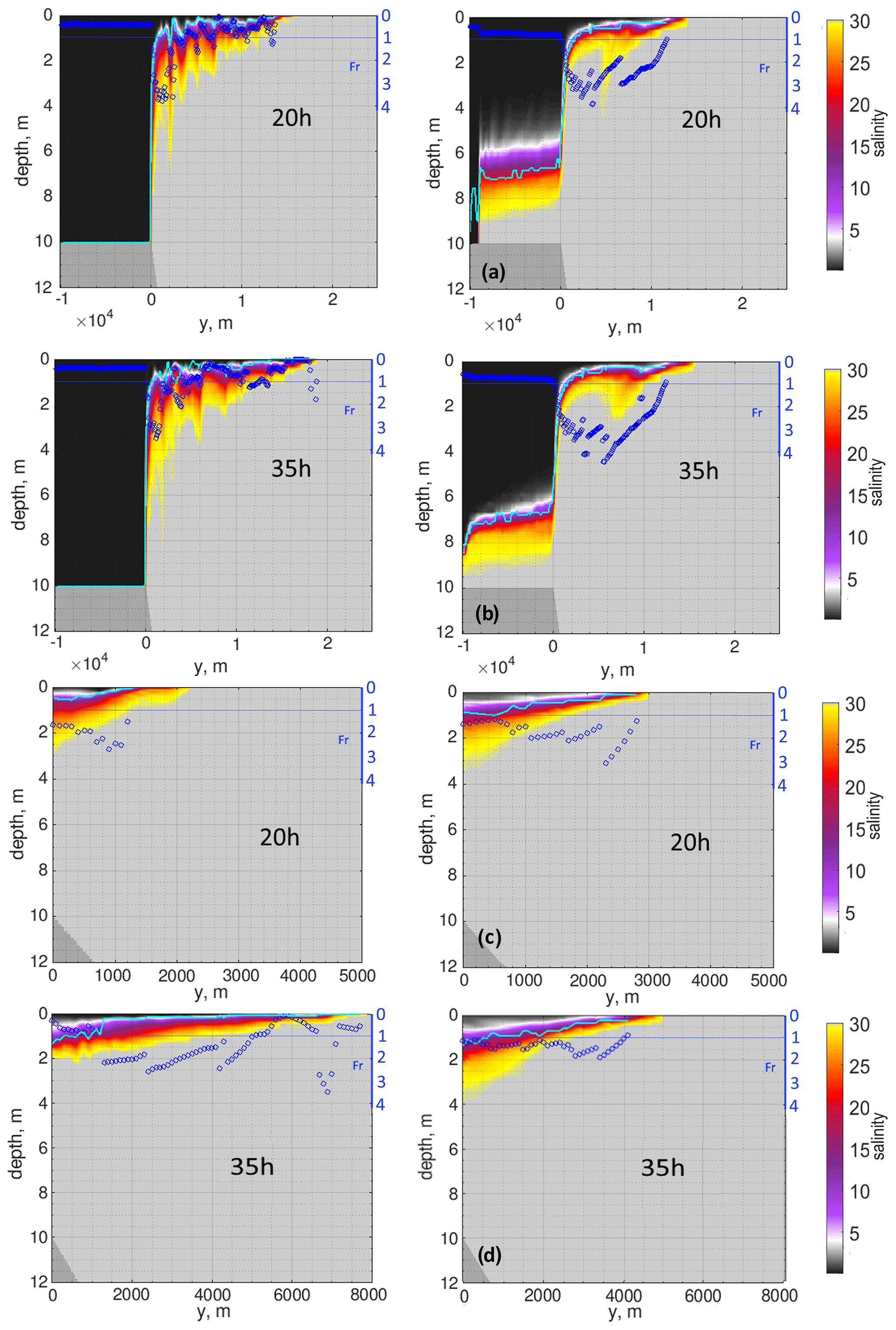
Figure 6 The salinity patterns, in practical scale, at cross sections based on runs 1 (left column) and 2 (right column) after one (20 h) and two (35 h) inertial periods. The upper two rows (a, b) illustrate the mouth transect, and the bottom two rows (c, d) illustrate the coastal current transect. The light blue line shows the thickness of the plume layer. The dark blue circles identify the approximate Froude numbers of the plume layer (see additional dark blue axes from 0 to 4 at the right side of each panel). The dark blue line shows the relative position of a Froude number equal to 1 for convenience.

In run 2, dense water penetrates into the river channel, showing a hydraulically controlled blunt-faced profile. We argue that the main reason for such a profile resides either in the flux-limiting scheme (which should be most active in this area) or in a relatively lower-order advection scheme. Indeed, the limiters are relatively diffusive horizontally in run 2 (compared to fct1 and fct2 options in FESOM-C), and the run used a second-order advection scheme. To confirm our assessment, we conducted run 4 with a more diffusive limiter definition, fct3 (see Sect. 2 for a description of the limiters), as well as run 5 with the second-order advection scheme and a relatively low diffusive limiter option, fct1. Figure 5, which shows the results after two inertial periods, confirms that the simulation yields a blunt-faced intrusion profile in both sensitivity runs. Naturally, both the lower-order advection scheme and the relatively diffusive limiters work toward a more diffusive solution. Interestingly, and as will be shown later, run 2 is characterized by small diahaline diffusivities (which indicates good performance) for the relatively higher salinities in the area of the hydraulic jump – compared to run 1 (Fig. 6) – despite the fact that the latter’s vertical advection scheme is of a higher order than that of run 2. Not only that, the surface salinity in run 2 is also slightly higher than it is in run 1 (Fig. 3).

Note that before the river flow reaches the mouth area during the initialization phase, both simulations take on an appearance typical of lock-exchange dynamics experiments. (We initially fill the river channel with river water.) However, this picture vanishes when the river flux reaches the mouth.

We diagnose the internal hydraulics of the model runs by computing the Froude numbers of the plume layer (Fig. 6). The Froude number is computed as $\frac{u_{\mathrm{b}}}{\sqrt{h_{\mathrm{b}}\cdot g^{\prime }}}$ (where h_b is the plume layer thickness, u_b the mean velocity within this layer, and g^′ the reduced gravity). The layer thickness is defined by the position of the maximum salinity gradient and maximum stress in runs 1–2 and 2, respectively. (The difference in definition is dictated by different discretization types.) But the plume layer border in both models still follows the isohaline with salinity ∼6.

The locations of the maximum Froude numbers differ between run 1 and run 2 (see Fig. 6). The difference can be traced to the velocity disturbances underneath the plume layer (Fig. 4), which are generated by the eddy vertical viscosity reacting to the shear stress at the near-surface; the latter is induced by a hydraulic jump. A pronounced salinity finger also appears in the area directly downstream of where the maximum Froude numbers occur. In run 1, the largest velocities (more than initial surface gravity wave speed) are more localized, and the maximum Froude numbers are found directly downstream of the mouth area.

5.2 Bulge and coastal current

Once the bulge (in idealized conditions) becomes nearly symmetric and tends towards instability, it becomes sensitive to any source of mixing: horizontal or vertical, physical or numerical. Therefore, the use of different advection schemes and limiters as well as time stepping results in different dynamics.

The ratio between the length (along-shelf spread) and width (offshore spread) of the bulge, called ellipticity (Avicola and Huq, 2003), is another parameter that indicates the presence of numerical mixing in the system. Generally, numerical mixing tends to reduce the bulge's external radius due to a decreasing salinity gradient (horizontal, vertical, or both) in the near-field or bulge zone and the resulting reduction in plume-associated offshore velocities. Numerical mixing leads to a deepening of the bulge and/or to a changed angle of impingement such that the center of the bulge gets closer to the coast: the bulge ends up being sliced off by the coastal wall. Numerical mixing therefore tends to increase the ellipticity. It thus comes as no surprise that in all configurations, including run 1, the ratio is too large compared to the expected number (Table 2). Interestingly, the alongshore length of the bulge in runs 1 and 2 is nearly within the range of analytically predicted values. In run 2 as in all others for which a second-order advection scheme and/or relatively diffusive limiters are used (i.e., runs 4, 5, 6, 10), the bulge is largely sliced off by the coastal wall. In run 1 (see Figs. 3 and 5), this effect is present to a smaller extent.

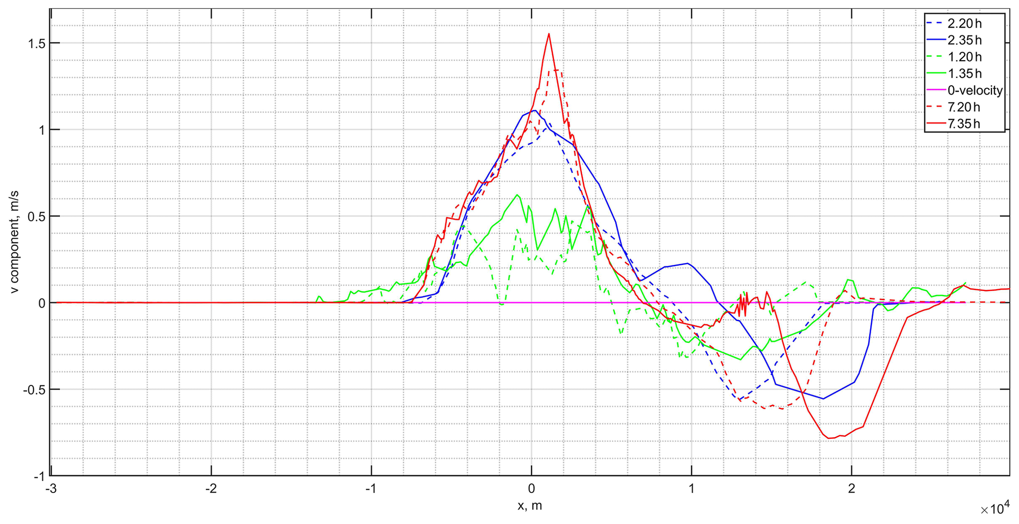
Figure 7 The surface v component of the horizontal velocity at the fixed y-axis position equal to the internal Rossby radius, ∼5.3 km, for different runs at 20 and 35 h.

Further details of the bulge structure can be derived from the v component of its horizontal velocity. Figure 7 shows the surface v component against x position at a fixed y that equals the internal Rossby radius (∼5.3 km, based on geostrophic depth). Although the line of a fixed y does not cross the bulge center, its approximate x position can still be identified from Fig. 7. Compared to the other runs on a triangular grid, run 1 depicts the bulge’s largest spread leftward from the mouth area. Consequently, the leftward displacement of the bulge’s center is found there; it is also located further from the coastline than it is in run 2.

In run 2, the bulge is less symmetric as expressed by the internal and external offshore radius; consequently, the coastal current's freshwater discharge is nearly twice what it is in run 1. The position of the second cross section in Fig. 2 at the coastal current is quite far from the mouth area. Therefore, while the front of the coastal current in run 2 reaches the cross section after 20 h, in run 1 the only part of the coastal current extending that far after 20 h is the nose area. This explains the difference in the numbers that pertain to the coastal current at 20 and 35 h. On average, the coastal current in run 1 and run 2 respectively transports about 25 % and 40 % of the initial freshwater discharge during the time period under consideration.

The position of the front of the coastal current can also provide a qualitative estimate of the level of numerical diffusion. Numerical mixing tends to move the bulge center closer to the coast, and hence a larger portion of fresh water enters the coastal current. The position of the head of the coastal current, or the magnitude of its discharge (compared to the analytical solution), can be used to diagnose numerical diffusion in the system (Fig. 5). Note that numerical diffusion levels may be even higher if the same small offshore restriction of the bulge parallels a weakly developed coastal current. In such a case, the bulge and the coastal current are excessively thick (see, e.g., run 6, Fig. 5).

Among our triangular discretizations, runs 1 and 3 are characterized by a larger bulge with a fresh surface as well as a slower and wider coastal current that transports less fresh water than it does in other runs and is closest to the analytical solution. Run 3 has slightly different fct-limiting details (it uses the fct2 option; see Sect. 2 for the details). Also, in run 1 as well as some of the additional runs the velocity and elevation fields (see, e.g., Figs. 3 and 5) depict the presence of physical instability at the frontal zones. However, the elevation fields there also depict some noise in the areas adjacent to the plume boundaries (Fig. 3d). The reasons for this noise are the spurious inertial oscillations present on triangular meshes in FESOM-C. Due to the absence of tracer diffusivity, specially designed filters (e.g., the biharmonic filter), and the expected low levels of numerical diffusion in run 1, such oscillations are not sufficiently damped there and are present in the simulated patterns.

5.3 Performance on rectangular grid

Here we consider runs 11, 12, and 13. Run 11 employs the same set of options as run 1 but is performed on a rectangular mesh (Table  1). As expected, on a rectangular mesh as in run 11, there are none of the inertial oscillations that appear on a triangular mesh due to the discretization type of FESOM-C. Noise occurs only where the grid resolution becomes sharply coarse (see Figs. 2, 8b). The plume in run 11 spreads nearly to the same position as it does in run 1. Due to the coarser grid, the coastal current’s nose extends a bit further here than in run 1. The surface, which is occupied by the plume, is nearly fresh everywhere in run 11. And there is no penetration of dense water into the river channel (Fig. 8a, c).

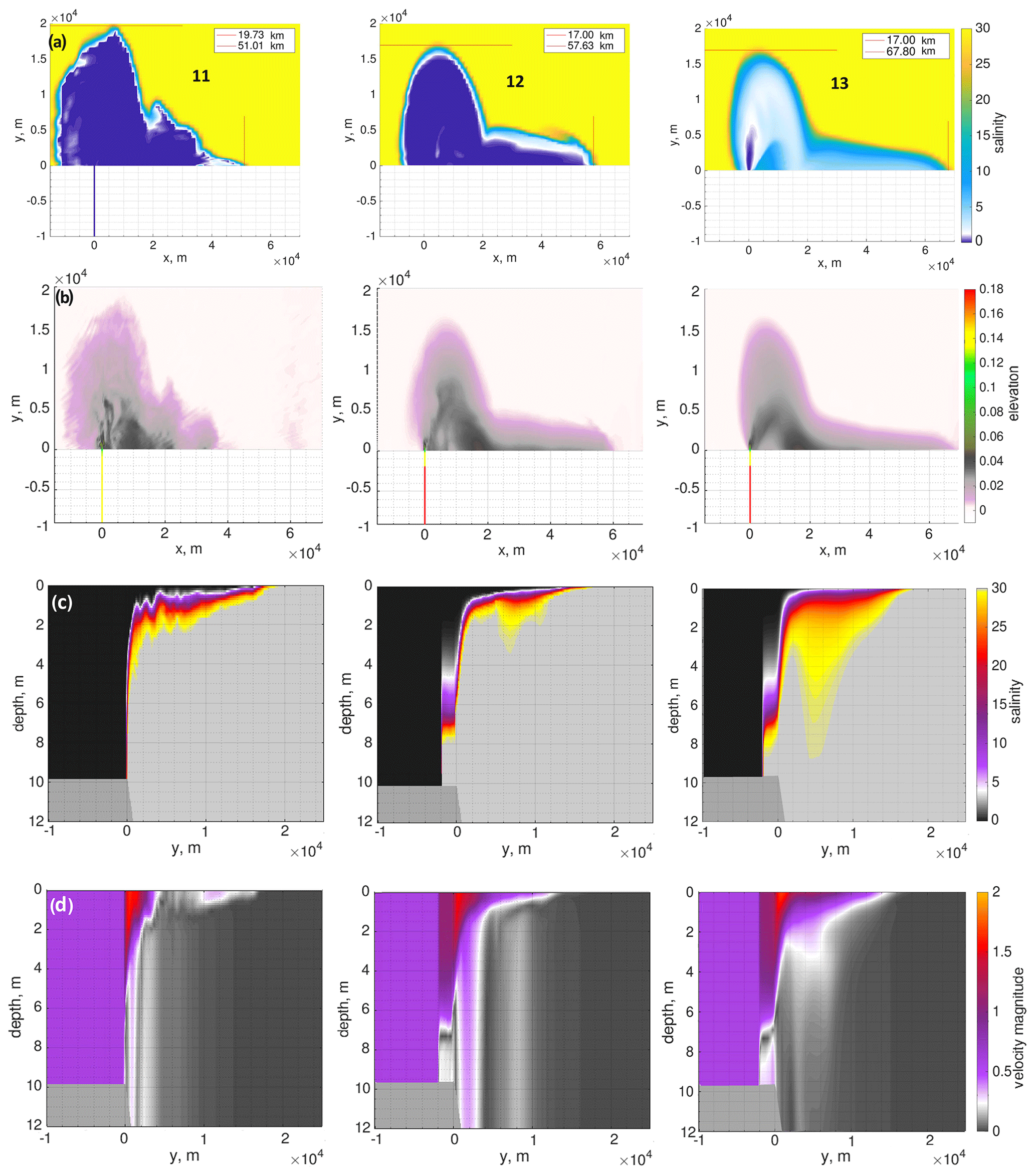
Figure 8 The results of run 11 (left panels), run 12 (middle panels), and run 13 (right panels) at 35 h performed on the rectangular grid: (a) surface salinity, in practical scale; (b) elevation (m); (c) salinity pattern at the mouth cross section, in practical scale; (d) magnitude of the velocity at the mouth cross section (m s⁻¹).

Run 12, which is characterized by the anti-diffusive limiter superbee, shows a generally smaller level of numerical mixing than the bulk of the runs presented on a triangular grid: the offshore spread of the bulge extends for 17 km; the surface layer occupied by the plume is generally fresh (Figs. 3, 5, 8). Both runs 11 and 12 simulate the ratios between alongshore and offshore spreads of the bulge, which are, relative to other runs anyway, close to the expected value of 1.3; they equal ∼1.4 and ∼1.5, respectively. It means that the bulge center is further offshore compared to other runs (Table 2).

Run 13 is characterized by nearly the same offshore plume spread as in run 12. However, the plume’s surface layer is characterized by a salinity of greater than 5, which means that run 13 is more vertically diffusive than runs 11 and 12. This happens due to use of Sweby's limiter in run 13, which is responsible for intense vertical mixing. Excessive vertical mixing is evident in Fig. 8c and d. Also, as expected, the coastal current propagates further in run 13 than it does in runs 11 and 12. Run 13 also shows penetration of dense water into the river channel; however, it has a slightly different interface profile than run 12 due to the different advection scheme of higher order employed in it (Table 2).

5.4 Numerical diffusivity and model performance

In the model runs wherein the physical diffusivity is set to zero any source of mixing of tracers is of numerical origin. In order to contrast it with physical diffusivity, run 7 with the physical diffusivity switched on (Table 1) will also be presented.

To carry out the numerical diffusion diagnostics presented above, we divide the available salinity range ([0, 30]) into 200 classes with the isohaline values $S_{\mathrm{i}}=S_{\mathrm{r}}+i\mathit{\delta }$ with i=1…200, where S_r=0 is a salinity of the river water and δ=0.15 is a size of the salinity class. For each salinity class, we calculated the total volume in the system and the isohaline area attributed to it after one and two inertial periods (Fig. 9). For simplicity's sake, we replace the isohaline area with its surface projection in all analyzed runs; the isohaline area is represented by the sum of the control areas of vertexes or elements depending on the discretization. With the exception of the isohaline configurations in the near-field zone, this is a reasonable assumption given that offshore spreading of the plume and its final deviation from the analytical solution – without additional forcing in the system – are mediated by diffusive processes (this issue is also presented in the Discussion section). We should mention that, for less diffusive solutions that tolerate meandering isohalines, the assumption would slightly overestimate the level of numerical mixing (Figs. 4, 6). Note that the true isohaline areas can readily be taken into account if a more accurate estimate is needed.

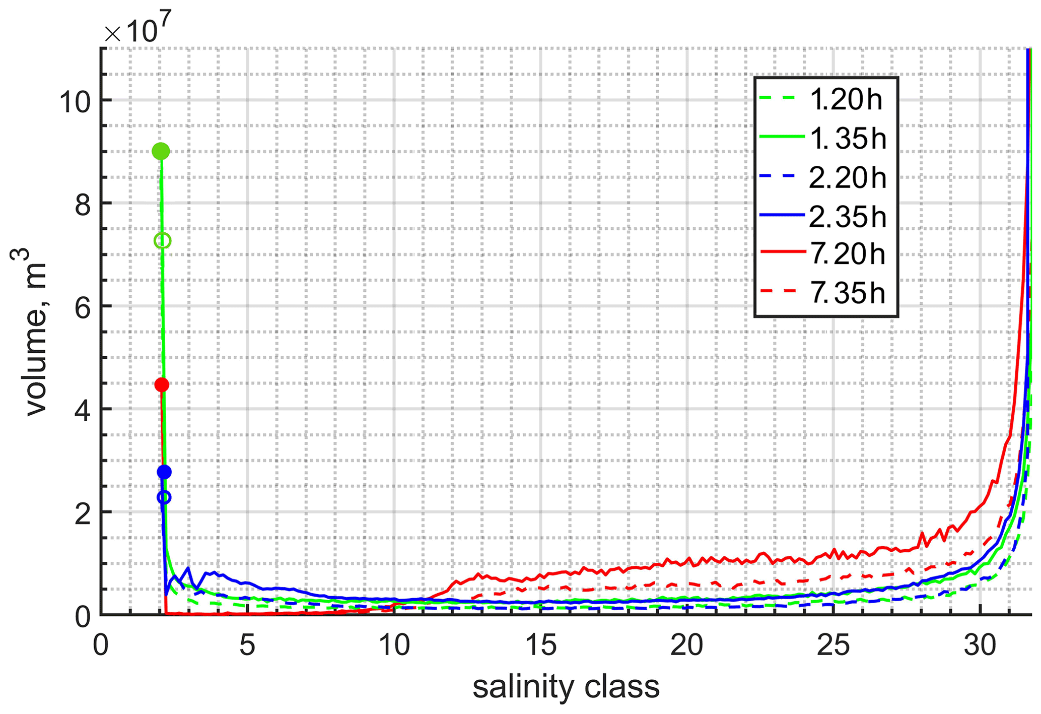
Figure 9 The salinity–volume diagram for runs 1, 2, and 7 at different time moments. The dashed and solid lines indicate the solutions at 20 and 35 h, respectively.

The salinity–volume diagram in Fig. 9 allows us to trace the total volume of each salinity class and, most importantly, the volume of the first freshwater class. Generally, numerical diffusion causes the appearance of volumes between the first and last salinity classes (which respectively contain fresh and shelf saline water masses) by reducing the volume of the first salinity class as well as (as in our case) that of the last salinity class. (No open boundaries are presented.) If the total volume of the freshwater class is less than the volume of the river channel (5×10⁷ m³), it means that the dense water penetrates into the river channel (Fig. 9).

The significant shift in the diagram can be attributed to the choice of the advection scheme or limiter; a lower-order advection scheme and/or relatively diffusive limiter tend to make the layer occupied by the plume saltier (Fig. 9): in run 2, the plume’s surface layer is a bit saltier than in run 1 and has a different structure. When eddy diffusivity is on (run 7), the volume of the higher salinity classes increases with time, whereas volumes remain stable (and very small) across the salinity classes characterized by salinities less than 10. This takes place because (in this case) we have a pronounced mixed layer with a salinity of about 10 in the near-field, bulge, and coastal current zones (Fig. 5). Also note that, despite the qualitative similarity of diagrams for runs 1, 11, and 12 (not shown), the total volumes of the first salinity class are more than 34 % larger at both 20 and 35 h time moments for the runs performed on a rectangular grid (runs 11, 12). Among all runs, runs 11 and 12 yield maximum freshwater volumes for the first salinity class. The realized fresh water thus largely stays fresh and does not replenish intermediate salinity classes in runs 11 and 12 to the same extent as other runs do. Runs 1 and 11 suggest that quasi-B discretization on the triangular grid can be a noticeable source of numerical mixing unless noise is suppressed by a filter. In the case of run 12, we may say that the anti-diffusion and anti-viscous superbee limiter (for tracer and momentum advection in GETM) is highly effective vertically in conserving the two-layer system with a pronounced interface between the plume and the quiescent layer (Fig. 8c, d).

It is known (e.g., Hetland, 2005; Burchard, 2020) that a larger isohaline area means less mixing for a given level of freshwater discharge through the isohaline. This fact is illustrated in Eq. (16). If we keep the diahaline freshwater discharge (total freshwater transport) F(S) constant and modify the isohaline area, which is situated in the denominator, the respective average diahaline freshwater flux, f(S), would increase. Increased diffusive fluxes, f(S), in turn mean increased mixing, which in our case is purely numerical. Also, the total volume of a particular class can be the same, while mixing levels differ from case to case due to different isohaline areas (Eqs. 14–16).

The volume of the first class can also be larger from one case to another in line with a higher numerical diffusivity level; this would apply, for example, where a plume spreads relatively little and remains relatively thick. To avoid a wrong interpretation of the salinity–volume diagram, one should consider the area of the isohalines (Fig. 10) for each different run.

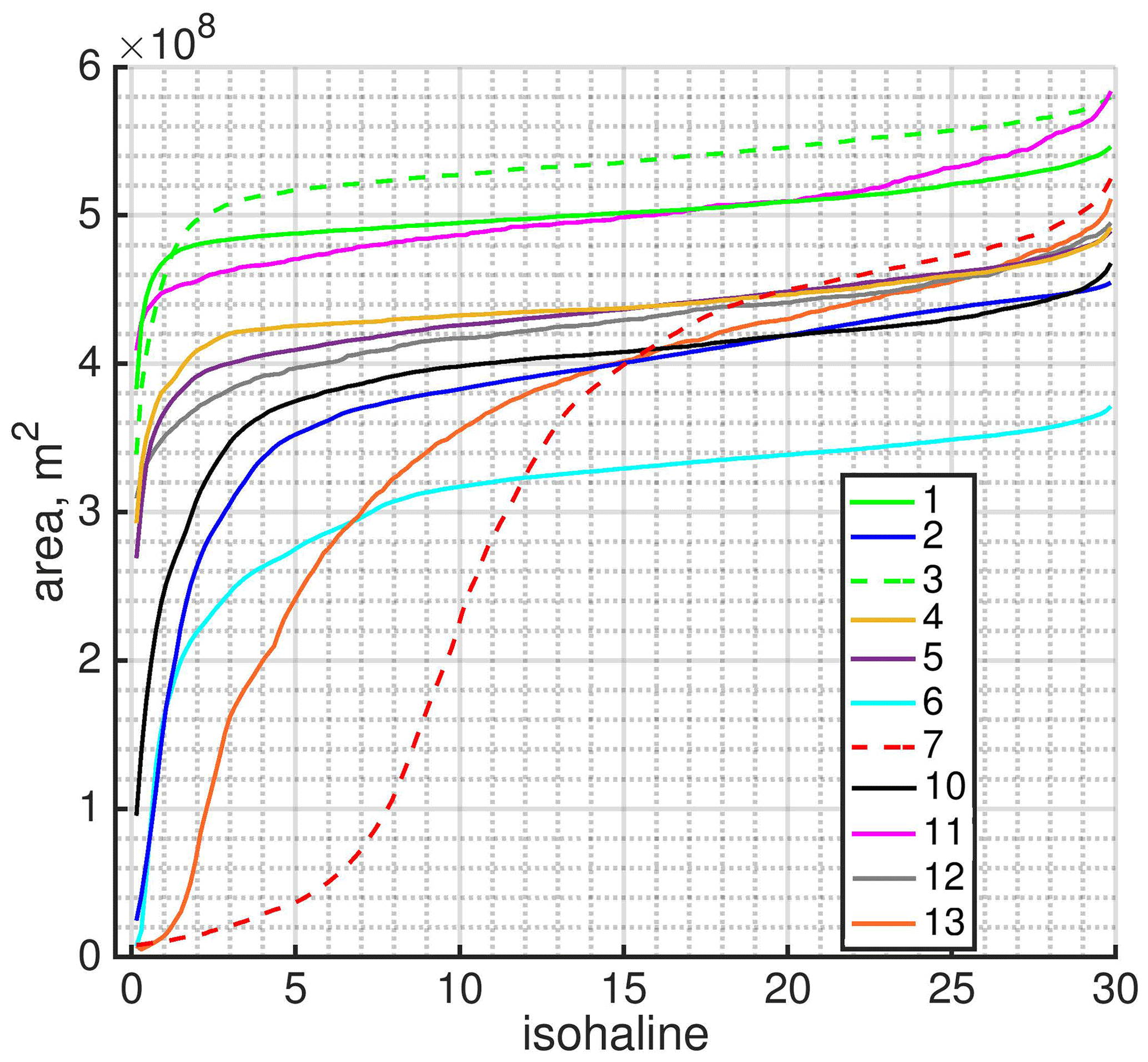
Figure 10 The mean (over the second inertial period) area of the surface projection of the isohalines for different runs.

Figure 10 illustrates the isohaline areas for different salinity classes. Except for run 7 in Fig. 10, which is characterized by the presence of physical eddy diffusivity, all curves have very similar shapes. These shapes reflect the fact that a two-layer system is being considered. The layer occupied by the plume is characterized by low salinities; it is not completely fresh due to the presence of numerical mixing. The plume layer can be characterized by the rapidly growing part of the curve. The curves, which are characterized by larger isohaline areas, mean larger offshore spreading of the plume. Even so, the coastal current in the more diffusive solutions can propagate faster; it is less restricted offshore paired with a bulge (e.g., Fig. 3). The shape of the curve for run 7 with eddy diffusivity turned on is an outlier. It signals the presence of the homogeneous salinity layer occupied by the plume, which is thicker compared to the same run with physical eddy diffusivity turned off (run 1). It is readily apparent that the limiters, which strictly preserve the monotonicity of the advection scheme, effectively reduce its order: the curves for runs 4 and 5 are nearly the same (Fig. 10, Table 1). Note that even use of the relatively close limiting options such as fct1 and fct2 (see Sect. 2 for the details), in the sense of expected numerical diffusion level, produces noticeably different dynamics. In particular, the curve for run 3 crosses the curve for run 1. It means that the plume layer is not so fresh in run 3 as in run 1, but the plume spreads a bit further offshore, which we can already see in Figs. 3 and 5. The vertical resolution also plays a large role: logically, a coarse vertical resolution introduces more numerical diffusion (see below); so, as a result, the curve for run 10 is significantly below the curve for run 5, and the layer occupied by the plume is saltier in run 10 compared to run 5.

Despite the fact that Figs. 9 and 10 indicate the diffusive processes taking place, several aspects remain to be clarified. For example, we have claimed that run 12 has what is among the largest freshwater volumes. However, in Fig. 10 the curve for run 12 starts below that for runs 1, 3, and 4. Also, additional steps are required before a quantitative estimation of the level of numerical mixing can be made. For this, we make use of the characteristics introduced in Sect. 4.

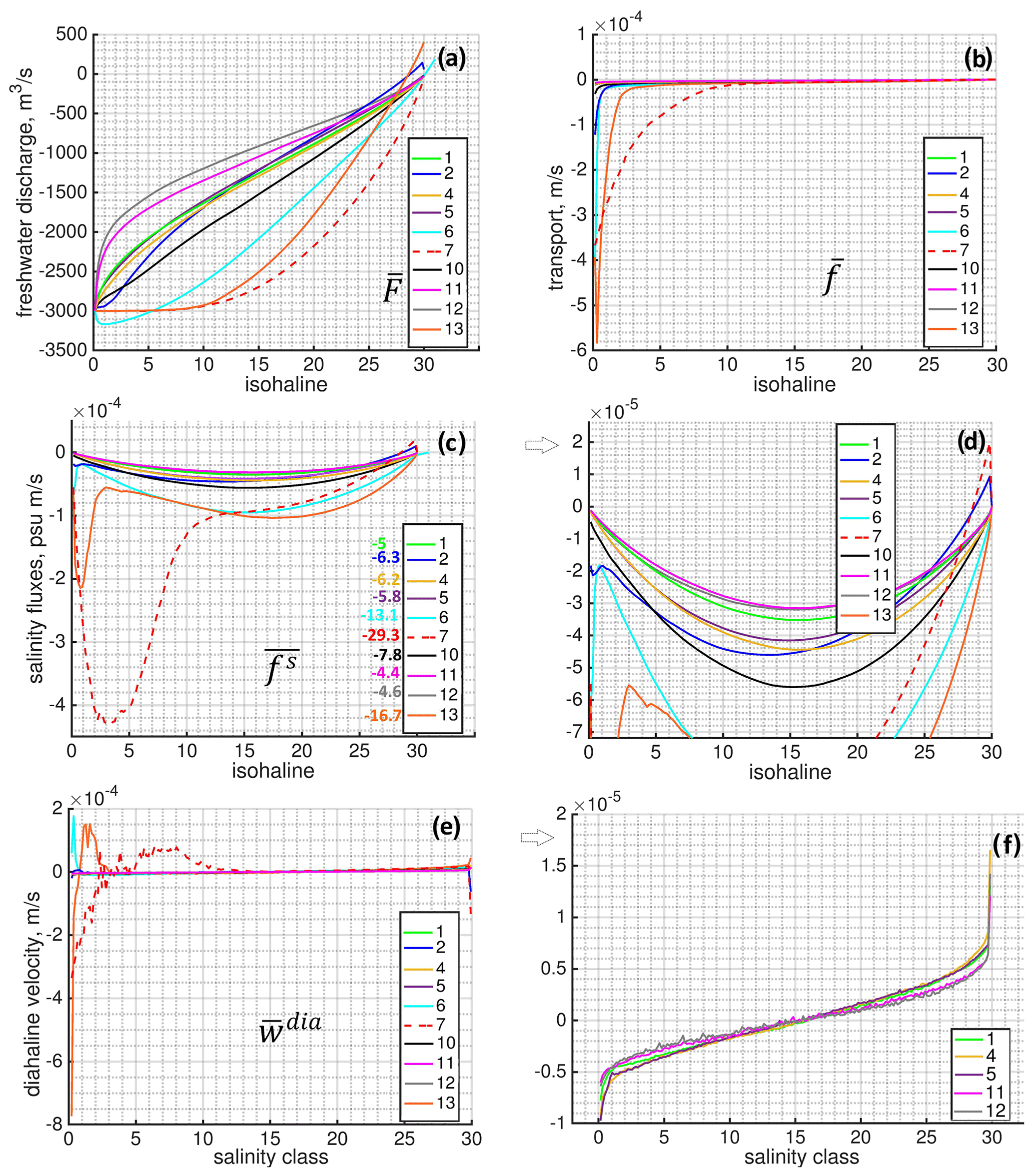
Figure 11 Analysis of numerical diffusion in the system: (a) total freshwater discharge through different isohalines, $\stackrel{\mathrm{‾}}{F}$ (m³ s⁻¹); (b) transport per unit area of each isohaline, $\stackrel{\mathrm{‾}}{f}$ (m s⁻¹); (c, d) total salinity fluxes through different isohalines, $\stackrel{\mathrm{‾}}{f^s}$ (psu m s⁻¹). The numbers indicate the sum of the salinity fluxes multiplied by 10³. (e, f) Diahaline velocities, ${\stackrel{\mathrm{‾}}{w}}^{\mathrm{dia}}$. In all pictures the characteristics are averaged over the second inertial period. In panels (b) and (e) the curves of runs 1, 4, 5, 11, and 12 are relatively close to each other.

We will start by considering the total salinity discharge through different isohalines divided by the salinity of the current isohaline (called “freshwater discharge”, Fig. 11a). Figure 11a allows one to trace the non-monotonic solution: run 6 accepts a discharge larger than $\sim -\mathrm{3000}$ m³ s⁻¹ because no limiters are introduced for the tracer advection scheme. For the less diffusive solutions, the absolute value of the discharge rapidly decreases, signalling that a relatively fresh surface layer is forming; it is growing and accumulating the fresh water. For run 7, the discharge is nearly equal to $\sim -\mathrm{3000}$ m³ s⁻¹ up through a salinity class of ∼10, so the plume forms a layer with a salinity of ∼10 even at the surface. The curve for run 13 has a similar shape. It signals that the limiter used for vertical advection works quite similarly to a physical vertical eddy diffusivity. The smallest numerical freshwater discharge can be attributed to the runs performed on a rectangular grid (runs 11, 12), with the best result attributed to run 12, meaning that the layer occupied by the plume is fresher than in other solutions. This explains the large freshwater volume in the system with a good (but relatively moderate) offshore spread of the plume as described above.

Figure 11b shows the mean transport through different isohalines: freshwater discharge through different isohalines (Fig. 11a) divided by the corresponding isohaline areas (Fig. 10). Transport naturally tends to decrease as the considered isohaline increases, but even so, the discharge can be the same (see, e.g., run 7 or run 13 in Figs. 10, 11a). Figure 11b sheds some light on vertical near-surface dynamics. For example, Fig. 11b shows that run 2 has a large cross-isohaline transport for low salinities. Therefore, despite its generally good performance, this run is characterized by a blurry surface layer (Fig. 3). We also see the principal difference between runs 7 and 13: transport through the freshwater isohaline is largest for 13 but then rapidly decreases, and there is no pronounced mixed layer as there is in run 7.

As we already mentioned, Fig. 11a can lead to a misunderstanding because of the total transport or freshwater discharge being considered. For a more transparent diagnostic, we draw the total salinity discharge through different isohalines, normalized by the isohaline area (Fig. 11c, d). In other words, Fig. 11c and d show the averaged diffusive salinity fluxes per unit area of the particular isohaline, which makes it easy to identify the more diffusive numerical solutions. With nonzero physical eddy diffusivity (run 7), the diahaline flux curve contains both physical and numerical components. Note that activating eddy diffusivity contributes to a smoother velocity field, so an “absolute” numerical diffusivity (with and without physical eddy diffusivity) is out of the question. But turning on physical eddy diffusivity in this particular test case will generally decrease numerical diffusivity (see the second local minimum of the solution). The numbers in Fig. 11c show the sum of the diahaline fluxes multiplied by 10³, so they demonstrate the level of numerical mixing for the current solution. Run 2 in comparison with runs 1, 4, and 5 demonstrates a higher diffusion level for the layer occupied by the plume, a lower level of diffusion for the higher salinity classes, and even anti-diffusion for the last salinity class. We came to a similar conclusion when we inspected surface salinity in Fig. 3. Run 10 clearly demonstrates that the coarser resolution causes a higher numerical mixing level and a blurry top plume-related layer. Here, we would like to stress that runs 11 and 12 have the lowest levels of numerical mixing. We have excluded run 3 with the fct2 version of the limiter from consideration here, since in run 3 the level of numerical mixing is very close to what was obtained in run 1 with the fct1 option (although slightly smaller, with a sum of salinity fluxes equal to $-\mathrm{4.9}\times {\mathrm{10}}^{-\mathrm{3}}$ psu m s⁻¹). Note that the fct2 option does not work nearly as well on a rectangular grid, which is a reaction to the rectangular grid’s relative coarseness (not shown; the sum of salinity fluxes is equal to $-\mathrm{7.2}\times {\mathrm{10}}^{-\mathrm{3}}$ psu m s⁻¹).

Some interesting and not obvious behavior of the system can be tracked by looking at the velocities through different salinity classes (Fig. 11d, e). It can be noticed that some solutions have a positive peak at the low salinity classes. Some runs, in particular, 1, 4, 5, 11, and 12, do not have this feature, demonstrating a nearly symmetric diahaline velocity pattern through salinity classes.

All models (e.g., runs 1, 2, and 12) accurately track the total freshwater volume in the system. Run 2 tends to underestimate the volume by roughly 2 %. This discrepancy is due to the weakly imposed river boundary condition in Thetis; the model itself is mass-conservative. The applied advection schemes with limiters (except run 6, which is not equipped with a limiter; see Table 1) are nearly monotone; the overshoots and undershoots for runs 1, 2, 3, 5, and 7–11 for salinity after 20 h of simulations are not more than 10⁻¹⁰ in practical scale. Runs 4, 12, and 13 are strictly monotone.

6 Discussion

In this section we discuss the sensitivity experiments and interpretation of the results. In particular, the effect of vertical resolution, penetration of the dense water into the river channel, and the role of vertical viscosity in the simulated plume behavior are clarified.

6.1 Vertical resolution

Runs 9 and 10 with a reduced number of sigma layers (20 instead of 40) reduce bulge offshore spreading by 4 %–8 % (Fig. 12). Also, even though these runs use different advection schemes (the hybrid MUSCL-type and Miura, respectively), they both generate a more saline surface layer compared to the reference runs 1 and 5 (Table 1).

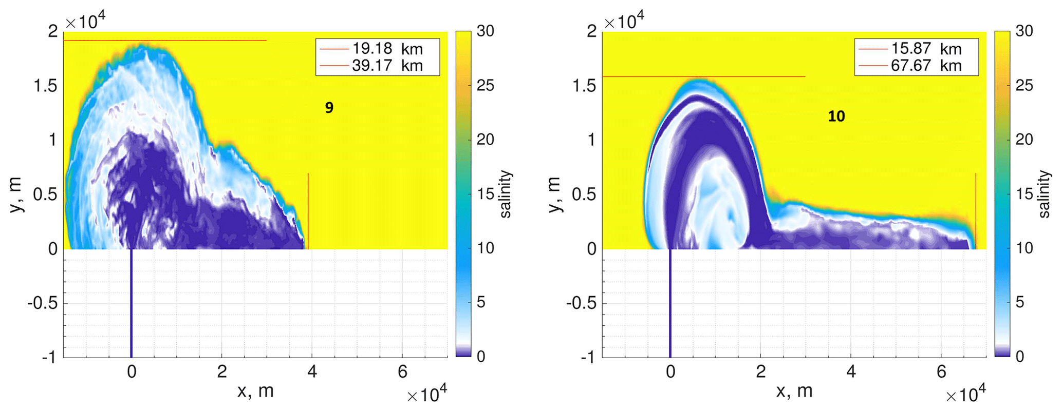
Figure 12 The surface salinity at 35 h, in practical scale, from runs 9 and 10 with a reduced number of sigma layers.

In the case of run 9, the bulge is slightly reduced offshore by 4 % compared to run 1 and not fresh at the surface. However, there is no pronounced redistribution of the discharge rates between the bulge and coastal current. Numerical mixing increases by 26 % in run 9 compared to run 1 (the sum of salinity fluxes is equal to $-\mathrm{6.3}\times {\mathrm{10}}^{-\mathrm{3}}$ psu m s⁻¹ in run 9).

In the case of run 10 there is a slightly thicker plume, a bulge offshore spread reduced by 8 %, and a coastal current propagating further compared to run 5. The numerical mixing increases by 35 % in run 10 compared to run 5 (the sum of salinity fluxes is equal to $-\mathrm{7.8}\times {\mathrm{10}}^{-\mathrm{3}}$ psu m s⁻¹ in run 10). We can note that the run with a relatively lower-order advection scheme (run 10 vs. run 9) reacts more strongly to the coarsening of the vertical resolution.

As expected, a coarser vertical mesh increases numerical mixing, which in turn modifies the plume behavior and final characteristics. It also restricts the minimum thickness of the plume. However, the effect remains moderate as the grid resolution is focused towards the surface.

6.2 Penetration of the dense water into the river channel

The dense water penetration into the river channel is sensitive to the details of the configuration. Since the resolution of triangular and rectangular grids is similar in the vicinity of a river mouth (Fig. 2), we concentrate on other factors. We have shown that numerical mixing related to limiters or upwind fluxes in the advection scheme can cause the penetration of the dense water into the river channel. However, in run 12 we observe penetration of dense water into the channel, although it has lower numerical mixing than run 1 in which penetration does not occur. Therefore, the relationship between numerical mixing and penetration depends on the source of numerical mixing. As we already mentioned the increased level of numerical mixing in run 1 compared to runs 11 and 12 is likely related to residual effects of spurious inertial oscillations supported by the discretization type.

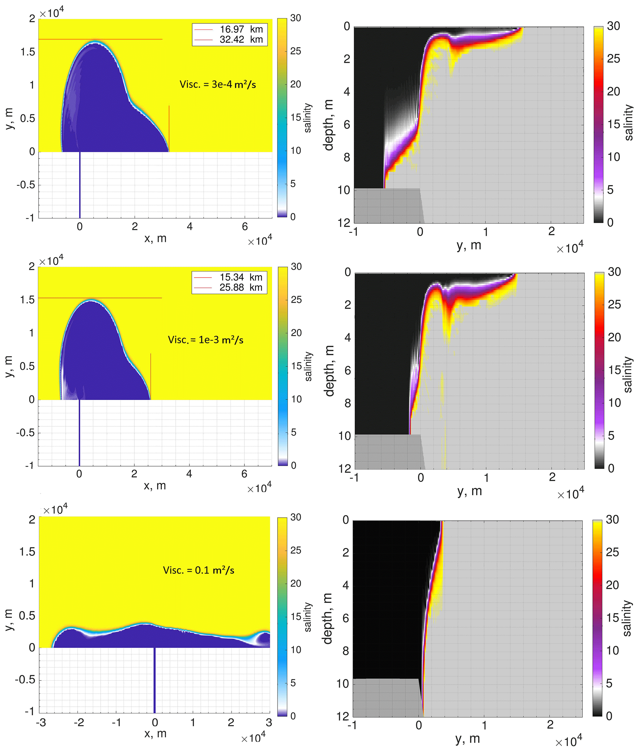
Figure 13 The surface salinity and salinity at the mouth transect at 35 h with different background viscosity levels (runs 8a, b, and c from top to bottom).

The area of hydraulic jump and shelf–river channel interface are also highly sensitive to the discretization of the momentum equation, in particular to calculation of the pressure gradient, momentum advection, and vertical viscosity. The latter is of prime importance. According to hydraulic theory the penetration of the dense water should occur if the liquid is inviscid. Obviously the vertical viscosity works oppositely to numerical mixing in this respect: relatively high viscosity blocks penetration of the dense water into the river channel. To show this, we carried out several sensitivity runs with only constant vertical background viscosity, and no limiting was applied in the vertical advection of momentum. Figure 13 visualizes some of them (runs 8a, b, and c; Table 1). This demonstrates the dynamics of the plume with a standard set of options on a triangular grid (as in run 1) except for the vertical viscosity (the horizontal viscosity was set to zero). If the viscosity equals $\mathrm{3}\times {\mathrm{10}}^{-\mathrm{4}}$ m² s⁻¹, the penetration takes place and has a typical lock-exchange profile. When the viscosity is increased to 10⁻³ m² s⁻¹, a much slower penetration is simulated. For an extreme value of background vertical viscosity of 0.1 m² s⁻¹, no penetration is seen.

Among all runs, only run 12 uses limiters for the advection of momentum. The superbee limiter used is characterized by locally anti-viscous (anti-diffusive) behavior. Runs 8a, b, and c show that higher viscosity inhibits the penetration of dense waters into the channel. Also, we have shown that in all cases with a relatively lower-order (up to second-order spatially) advection scheme the penetration occurs and has a blunt-faced profile (runs 2, 5, 6, 12; Figs. 3, 5). The results suggest that the penetration occurs in run 12 due to the combination of a second-order tracer advection scheme and anti-viscous limiter for the advection of momentum.

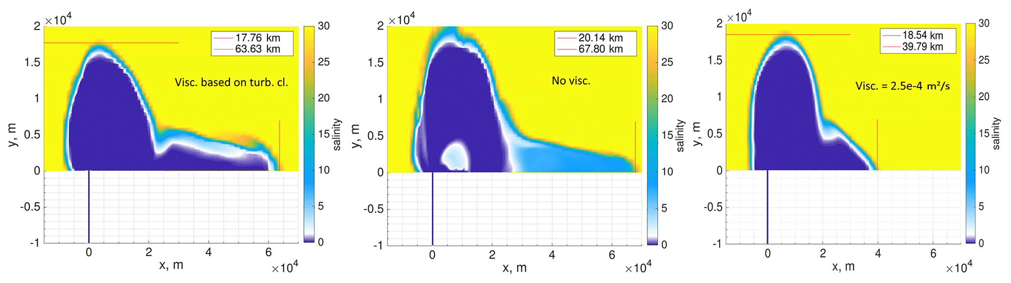
Figure 14 The surface salinity, in practical scale, at 35 h as a result of runs 12c, 12b, and 12 (see Table A1; discharge rate is 3900 m³ s⁻¹).

In addition, we investigated the influence of the river discharge on the penetration of dense waters. For all the runs wherein penetration occurred we increased the discharge to 3900 m³ s⁻¹. As predicted by Armi and Farmer (1986) (see Sect. 3 for some details) in this case the penetration of dense waters did not occur in all simulations. Also, we should note that in the absence of bottom friction the penetration did not influence the plume characteristics considered by us. For example, run 12 has slightly larger offshore spread – about 1 km – compared to the old realization, as it should according to the analytical solution (Fig. 14).

6.3 Viscous processes

This subsection is largely based on an additional set of experiments with a slightly increased discharge of 3900 m³ s⁻¹ and a constant vertical viscosity equal to $\mathrm{2.5}\times {\mathrm{10}}^{-\mathrm{4}}$ m² s⁻¹ (Table A1). The slightly larger discharge is preferable because it results in a thicker plume layer. The analytical prediction for the major plume characteristics in this case is given in brackets in Sect. 3.

The experiments described above make clear that the vertical viscosity and the details of the momentum equation discretization play a significant role in the simulated plume dynamics. The analytical solution approximates the flow as a two-layer system with a plume layer having a uniform shear and a motionless lower layer. If the vertical background viscosity in simulations is lower than $\mathrm{2}\times {\mathrm{10}}^{-\mathrm{5}}$ m² s⁻¹ (the horizontal viscosity is set to zero), all models participating in this study cannot preserve the two-layer system; the coastal current has an average salinity above 10 and anomalously high speed. An example is given for run 12 (Table A1 and Fig. 14, middle), which gives one of the best results but still contains these artifacts. It could also be that stability conditions cannot be met for a reasonable time step above 1 s for the baroclinic mode. The reason is the presence of numerical mixing in the system, which dilutes the thin freshwater layer, and other numerical inaccuracies, which in this case have pronounced consequences. With the vertical viscosity of about 10⁻³ m² s⁻¹ the solutions are significantly damped: the offshore spread of the plume is restricted together with a reduced coastal current, and the plume layer is too thick (e.g., Fig. 13). If the viscosity has an order of 10⁻⁴ m² s⁻¹, all solutions are relatively close to each other compared to the runs with eddy viscosity turned on in terms of the bulge size and strength of the coastal current (Fig. A2). Note that with this level of background viscosity FESOM-C results on triangular and quad meshes (runs 1 and 11 in Table A1) are also much closer to each other, suggesting that the noise triggered by the triangular grid in FESOM-C is already partly damped or not generated in such conditions. The eddy viscosity calculated based on turbulence closures (see, e.g., runs 1b, 12c; Table A1) in the area of plume spreading has a mean value of the order of 10⁻⁴ m² s⁻¹, with the maximum reaching an order of 10 m² s⁻¹. This naturally means that the background value of the order of 10⁻⁴ m² s⁻¹ is too small and too large for the different subareas compared to the eddy viscosity based on turbulence closures (see, e.g., Fig. A1).

For the runs with only background viscosity the level of numerical mixing and agreement with the analytical solution are not in a direct correspondence: in this case the differences between the runs are largely reflected in the volume of intermediate salinity classes, which are to a degree separated from the surface dynamics if there is no eddy viscosity. So, the new run 6 has a fresher surface and larger offshore spread compared to run 2, but a higher level of numerical mixing (see, e.g., Figs. A3, A4). Also, run 9 with a number of vertical levels 2 times smaller shows better performance with respect to the level of numerical mixing and offshore spread compared to run 1 with the same set of options, but with the larger number of layers. Run 12 with anti-viscous and anti-diffusive limiters shows the best performance among all runs in the sense of numerical mixing (Fig. A4).

We note that the thickness of the plume layer at the coastal current has a different structure in all these runs compared to the runs with eddy viscosity: in particular, it does not reach a maximum near the wall as in analytical and laboratory studies (see Fig. A2). An additional issue is the absence of the bulge symmetry predicted by the laboratory studies (they were conducted with viscid liquids), in particular an offshore extent of the bulge that is too large compared to its alongshore size. All numerical solutions have different built-in viscosity and it is hardly possible to find one value of background viscosity which would account for the difference without damping the dynamics significantly. When the eddy viscosity is turned on, the details of momentum equation discretization become less important (as in the case of eddy diffusivity, the presence of physical eddy viscosity makes the level of numerical viscosity smaller) and the level of numerical mixing can be estimated by offshore plume position. The last point was crucial for the current test case, which has a focus largely on numerical diffusivity. Therefore, we used the turbulence closure for eddy viscosity instead of constant viscosity in all runs beyond the ones presented in Sect. 6. The choice of turbulent closure for the vertical eddy viscosity coefficient impacts the way different zones function. For this reason we highly recommend employing second-order turbulence models (e.g., see review in Umlauf and Burchard, 2005) to be able to carefully compare results with the results presented here.

We mention that the presence of supercritical conditions in addition to numerical mixing can be a reason for the underestimations of the bulge offshore spreading by the numerical solutions. However, the analytical solution is given for a wide time range (one inertial period); this ensures the feasibility of the numerical solution to reach an analytical one. The prime results of runs 11 and 12 demonstrate this (Fig. 8).

6.4 Model type

In the test case three models with different discretizations have been applied: most runs were carried out with the FESOM-C, a quasi-B-grid finite-volume model with different advection schemes and flux limiters. Run 2 was performed using the Thetis DG finite-element model that uses a second-order advection scheme and geometric slope limiters. Runs 12 and 13 were carried out with the C-grid GETM. The most salient differences in the simulations, however, were due to the order of the advection scheme and the quality of the limiters, not the model type itself. However, some differences in the dynamics can be found due to the model and discretization type. In the case of the quasi-B-grid finite-volume model the velocity field exhibits noise on triangular grids. The latter issue is well known and can be dealt with using a biharmonic filter operator (e.g., Danilov and Androsov, 2015). The DG model is less diffusive in the layer not occupied by the plume and more diffusive in the plume layer compared to the GETM and FESOM-C runs with the second-order (horizontally) advection scheme. As a result, in the Thetis run the surface is saltier and smoother, but the system has a pronounced two-layer character and the layer occupied by the plume is not thick. While there is no obvious explanation for this behavior, most probably it is caused by a combination of the vertical discretization, current advection scheme, and the geometric DG limiter. More experiments are needed in the same frame to further clarify details.

Table 3 The description of runs and their results with respect to changes in the advection scheme and limiter types. The discharge in all setups was equal to 3000 m³ s⁻¹; 40 vertical layers were used, and eddy viscosity coefficient was calculated based on a second-order turbulence model (k−ϵ style) (FV – finite volume, DG-FEM – discontinuous Galerkin finite-element method).

7 Conclusions

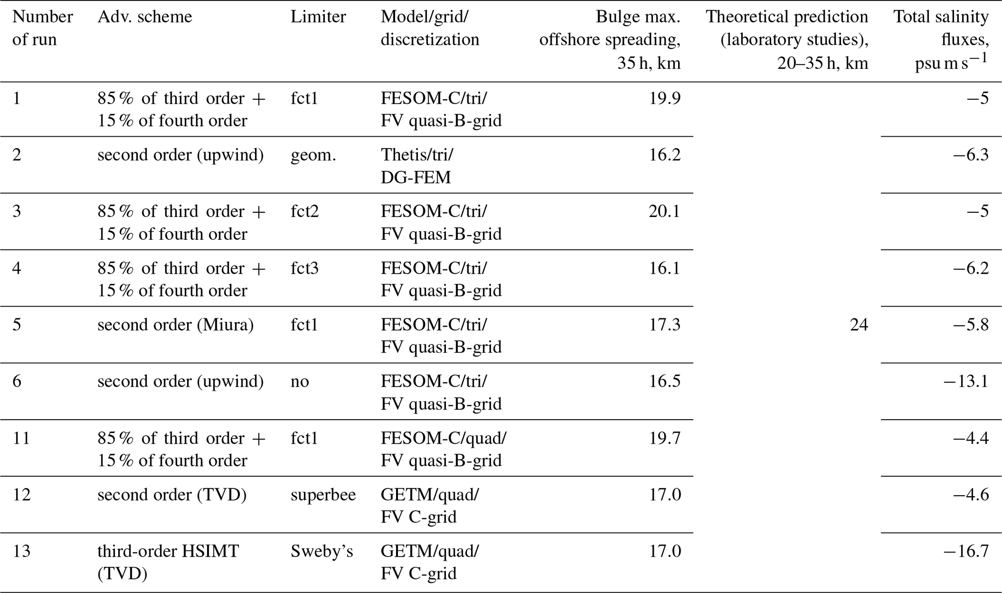
As expected, all models reproduce the four prototypical zones shown in Fig. 1, preserve freshwater volume in the system, and are stable. However, substantially different dynamics in each zone can be obtained using the same model but with different transport schemes. The major result of our comparative study is that accuracy in reproducing the analytical solution depends less on the applied model discretization or grid type than on the advection scheme. Table 3 illustrates how the choice of an advection scheme and limiter affects the performance. All runs listed there were carried out with the same number of vertical sigma layers and the same turbulence closure for vertical viscosity (eddy diffusivity is set to zero). Table 3 presents two final characteristics: the maximum offshore bulge spreading and total salinity fluxes after two inertial periods, enabling a better evaluation of the simulation. The total salinity fluxes characterize the net level of numerical diffusion in the system, or how closely the system adheres to the expected two-layer system with only two salinity classes. The smaller the absolute value of salinity fluxes, the lower the level of numerical mixing in the considered simulation.

In runs wherein eddy vertical viscosity is turned on, the level of numerical diffusion and simulated plume characteristics are interrelated (Table 3, Sect. 5). If numerical mixing is larger, we get a smaller bulge offshore extent, a thicker plume, a bulge center closer to the coast, and a larger coastal current discharge. However, although they are related, they complement each other: the bulge spreading largely characterizes the horizontal part of the dynamics, whereas total salinity fluxes characterize the vertical. When eddy viscosity is replaced by a constant background value (Sect. 6.2, 6.3), horizontal and vertical dynamics become less dependent.

The order of accuracy of a given scheme is as important as the type of limiter. The fct1, fct2, geometrical, and superbee limiters outperformed fct3 and Sweby's limiters in the sense of two considered characteristics (Table 3). In general, the superbee limiter, with its anti-diffusive properties, can be marked as the best limiter and the Sweby's as the worst (however, only in the vertical dimension) for the considered task. Among the considered advection schemes, the best performer was a hybrid MUSCL-type advection scheme (third to fourth order). Combined with the fct1 limiter, it gives the best result for the runs for which eddy vertical viscosity was calculated based on turbulence closure. However, for a highly accurate advection solution, noise may appear, which is attributed to the discretization type (or of other origin). Among the tested second-order advection schemes, the Miura and TVD schemes performed better than the upwind scheme.

In realistic cases, many other factors, such as physical mixing, influence the plume dynamics in addition to the numerical mixing. We therefore refrain from selecting the best scheme based solely on the results presented above. However, knowledge of the extent to which numerical mixing may affect the solution is an important preliminary step, and we hope that the approach of this paper will be of interest to other modelers.

Appendix A: Additional runs

Table A1 The description of the additional runs; the discharge is equal to 3900 m³ s⁻¹ (other setup details are the same).

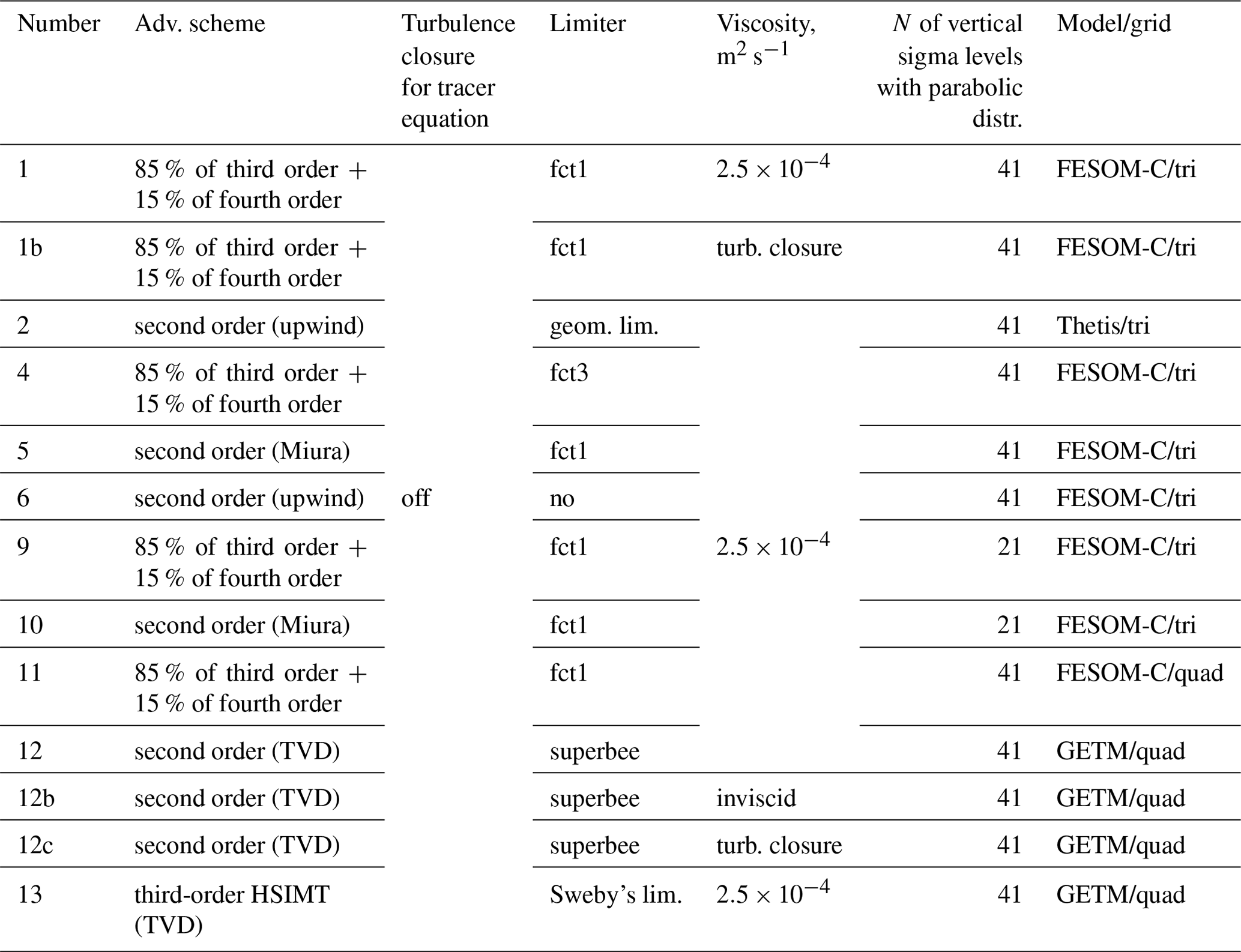
Figure A1 The surface salinity, in practical scale, at 35 h as a result of runs 1 (a) and 1b (b) (see Table A1 for the run details).

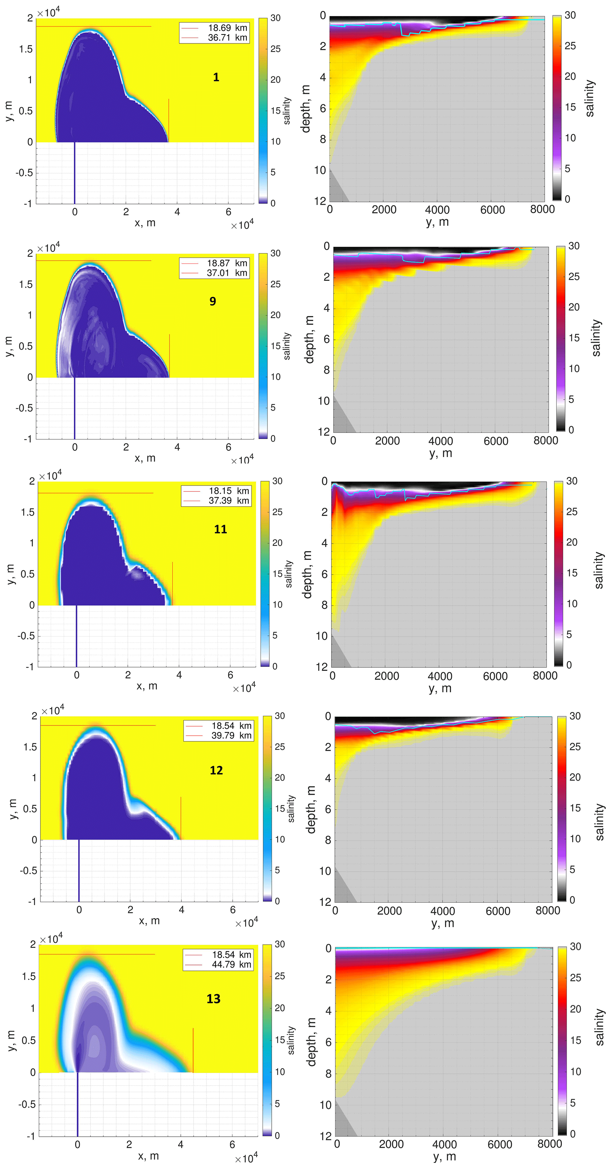
Figure A2 Salinity, in practical scale, as a result of the different runs at 35 h at the surface (left panels) and coastal current transect (right panels) (see Table A1 for the run details).

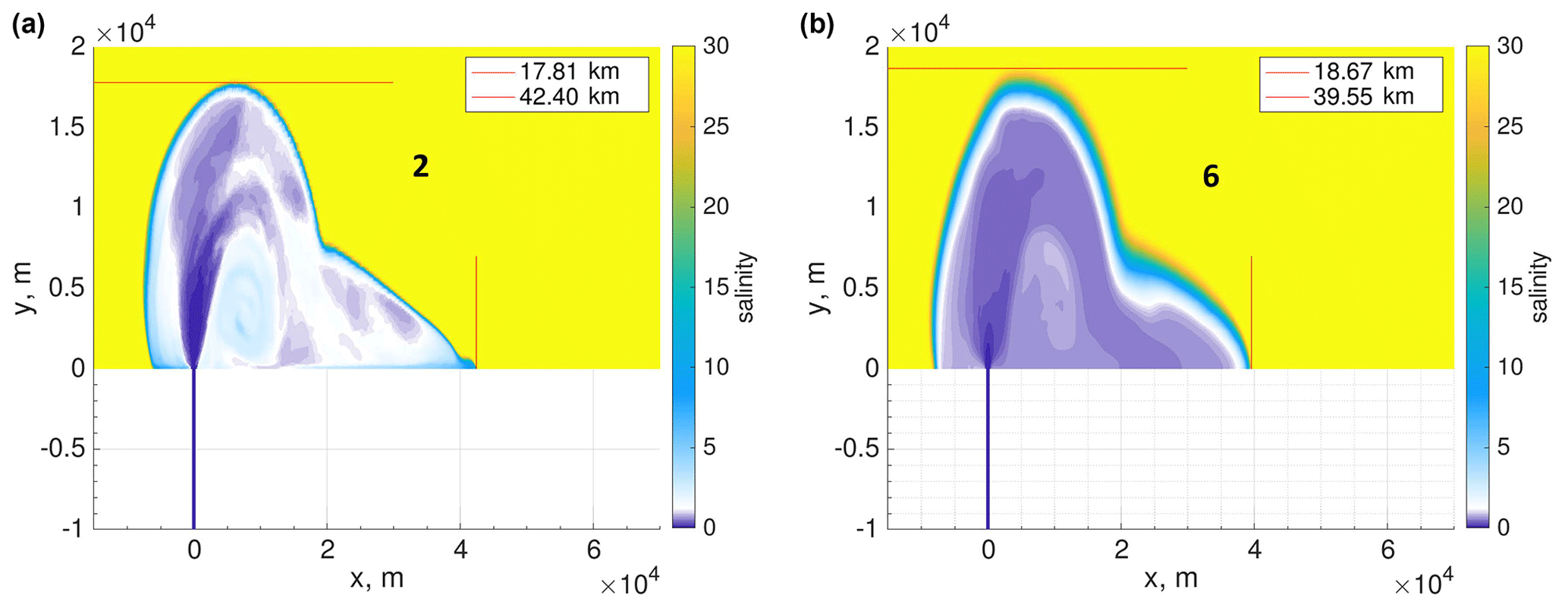
Figure A3 The surface salinity, in practical scale, at 35 h as a result of runs 2 (a) and 6 (b) (see Table A1 for the run details).

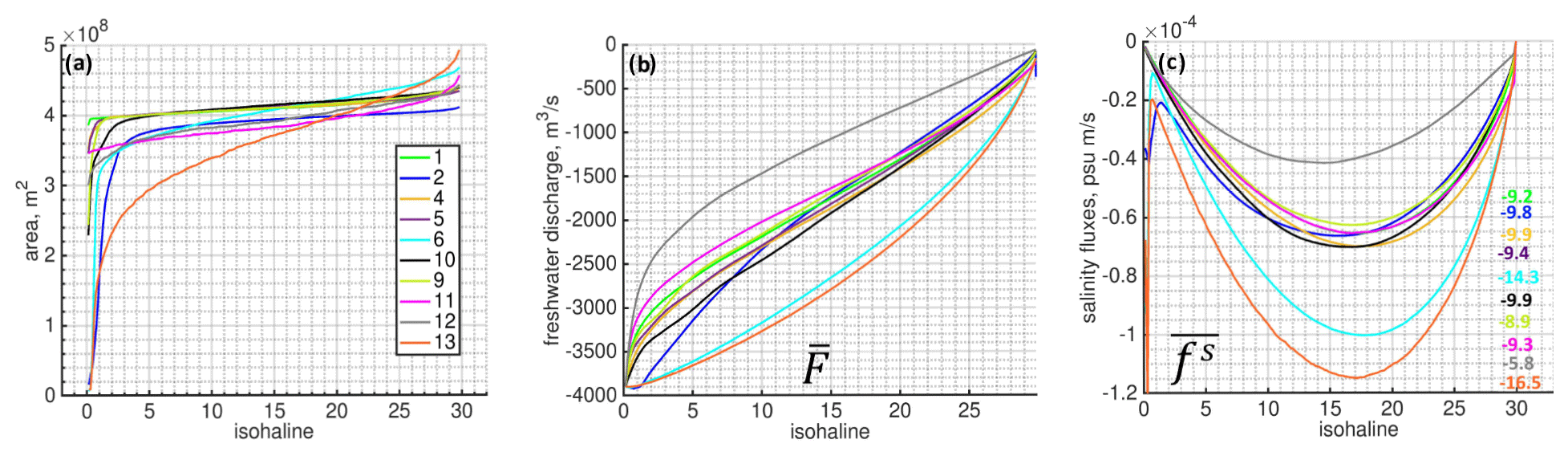
Figure A4 Analysis of numerical mixing in the system performed for the different runs (Table A1): (a) isohaline areas; (b) total freshwater discharge through different isohalines, $\stackrel{\mathrm{‾}}{F}$ (m³ s⁻¹); (c) total salinity fluxes through different isohalines, $\stackrel{\mathrm{‾}}{f^s}$ (psu m s⁻¹). The numbers indicate the sum of the salinity fluxes multiplied by 10³. In all panels the characteristics are averaged over the second inertial period.

Appendix B: User information

B1 Summary of the test case, major points

The test case presents a river–shelf system: there is a source of fresh water and momentum separated from the shelf by a perpendicular river channel, and there are no additional forcing terms and no open boundaries (i.e., the total water volume entering the domain stays there). Models of eddy diffusivity should be set to zero, which makes the diagnostic of the numerical mixing very transparent and allows us to consider the plume behavior at some aspects in terms of a two-layer paradigm (see Sect. 3 for details). The eddy vertical viscosity should be calculated based on a second-order turbulence model (see, e.g., review in Umlauf and Burchard, 2005), preferably the k−ϵ model. The test case assumes the usage of a linear equation of state in which the density difference between the river and shelf water masses is equal to 23.01 kg m⁻³. However, if the user does not have access to the equation of state and would like to try a non-monotonic advection scheme or advection schemes with flexible limiters, we suggest, for example, using a salinity of 2 and 32 for the river and shelf waters, respectively, to avoid negative salinity in the numerical solutions at the frontiers areas; the most important aspect is to keep the density difference between the river and shelf water masses (23.01 kg m⁻³). In this case the visualizations should be the same as presented in the current article, and only the color bar or salinity range should be shifted toward high salinity. The bottom friction should be turned off. In the simulation, 40 sigma layers (41 levels) should be prescribed with the parabolic distribution defined by Eq. (2). If the same vertical grid cannot be utilized, running of a test case still makes sense; however, the numerical diffusivity level and output plume characteristics given in the article (Tables 2, 3) should not be used for the intercomparison.

The total simulation time is 35 h and the grid contains ∼ 76×10³ triangles ($\sim \mathrm{60}\times {\mathrm{10}}^{\mathrm{3}}$ rectangles), so the task can be calculated within an appropriate time even by models running on laptops.

The further details of the setup are specified in Sect. 2.

B2 Summary of the analytical solution

After ∼8.2 h of the total simulation time the plume is expected to start turning right at an approximate distance of 5 km from the coast. After 20–35 h the offshore spread of the bulge should reach ∼ 24 km. The surface layer occupied by plume should be fresh.

The estimated maximum and minimum thicknesses of the coastal current are about 1.8 and 0.9 m, respectively, and maximum velocity (the near-wall speed in the layer occupied by the plume) is in the range from 0.45 to 0.64 m s⁻¹. The cross-shore width of the coastal current can vary from 3.75 to 12 km after one to two rotation periods.

The surface salinity, the profile of dense water intrusion into the river channel (if present), its speed, the coastal current's discharge rate, offshore spread, and asymmetry or the characteristic impingement angle of the bulge can all be considered indirect measures of numerical mixing. However, the simplest way is to consider the offshore spread of the bulge and its surface salinity. Numerical mixing tends to reduce the offshore spread of the bulge, make it deeper, and increase its surface salinity. In addition, the bulge center tends to shift towards the coast, thus lowering the impingement angle and increasing the strength of the coastal current.

B3 Output requirements and corresponding definitions

In the current test case we are focusing on the final characteristics of the plume spreading, in particular the position of the lift-off zone, bulge characteristics at a given time (offshore, nearshore-wide, and alongshore-long), depth of coastal currents, cross-front width, and velocity. These characteristics should be extracted at two time moments: 20 and 35 h from the beginning of the simulation time (20 h is approximately the time it takes for fresh water to reach the mouth area, plus one inertial period; Fig. 1).

For users interested in detailed analysis of the model performance, we recommend filling in the Table 2 and performing full numerical diffusivity analysis or at least reproducing the metrics in Fig. 11c.

Tracing the level of numerical diffusive transport and checking the prediction against the analytical solution require the following output: (a) surface velocities as well as elevation and 3D salinity fields and (b) velocity profiles for two transects (Fig. 2) at the specified times. The calculation of the mean isopycnal areas within the second inertial period can be simplified to the calculation of the surface projection of each considered isohaline (sum of vertex or, depending on the type of discretization, element or edge control areas, where particular salinity S is present at any depth) at two time moments – 20 and 35 h – and its further averaging. The full range of salinity values should be split into 200 salinity classes with the salinity difference between neighboring classes equaled to 0.15. The first and last classes can be larger if a non-monotonic advection scheme is used (it is important to cover the whole salinity range presented in the model).

The layer thickness occupied by the plume should be defined by the maximum salinity or velocity gradient depending on the discretization (one field can be noisier than another); the shape of the bulge is identified by the surface plot of salinity: the salinity contour 29 in practical scale should be considered a border to identify the bulge spread and coastal current position.

The shortest version of the analysis includes only surface visualization of the salinity at 35 h. Ideally in the system after 35 h the bulge offshore extent should be more than 24 km (and the coastal current nose should not reach 40 km on the x scale), and the layer occupied by a plume should be fresh. The minimum acceptable result is that the bulge spreads offshore at about 16 km (and the coastal current extent is less than 70 km).

To verify volume conservation the total water volume in the system should be checked after 20 h. An increase in volume compared to the initial state should be 0.2052 km³ plus the amount of fresh water which flows during the first hour when river discharge is ramped up – 0.0054 km³.