the Creative Commons Attribution 4.0 License.
the Creative Commons Attribution 4.0 License.
 | 15 Nov 2021
DRYP 1.0: a parsimonious hydrological model of DRYland Partitioning of the water balance
E. Andrés Quichimbo
Michael Bliss Singer
Katerina Michaelides
Daniel E. J. Hobley
Rafael Rosolem
Mark O. Cuthbert
Dryland regions are characterised by water scarcity and are facing major challenges under climate change. One difficulty is anticipating how rainfall will be partitioned into evaporative losses, groundwater, soil moisture, and runoff (the water balance) in the future, which has important implications for water resources and dryland ecosystems. However, in order to effectively estimate the water balance, hydrological models in drylands need to capture the key processes at the appropriate spatio-temporal scales. These include spatially restricted and temporally brief rainfall, high evaporation rates, transmission losses, and focused groundwater recharge. Lack of available input and evaluation data and the high computational costs of explicit representation of ephemeral surface–groundwater interactions restrict the usefulness of most hydrological models in these environments. Therefore, here we have developed a parsimonious distributed hydrological model for DRYland Partitioning (DRYP). The DRYP model incorporates the key processes of water partitioning in dryland regions with limited data requirements, and we tested it in the data-rich Walnut Gulch Experimental Watershed against measurements of streamflow, soil moisture, and evapotranspiration. Overall, DRYP showed skill in quantifying the main components of the dryland water balance including monthly observations of streamflow (Nash–Sutcliffe efficiency, NSE, ∼ 0.7), evapotranspiration (NSE > 0.6), and soil moisture (NSE ∼ 0.7). The model showed that evapotranspiration consumes > 90 % of the total precipitation input to the catchment and that < 1 % leaves the catchment as streamflow. Greater than 90 % of the overland flow generated in the catchment is lost through ephemeral channels as transmission losses. However, only ∼ 35 % of the total transmission losses percolate to the groundwater aquifer as focused groundwater recharge, whereas the rest is lost to the atmosphere as riparian evapotranspiration. Overall, DRYP is a modular, versatile, and parsimonious Python-based model which can be used to anticipate and plan for climatic and anthropogenic changes to water fluxes and storage in dryland regions.
- Article
(4101 KB) - Full-text XML
-
Supplement
(258 KB) - BibTeX
- EndNote


Drylands are regions where potential evapotranspiration far exceeds precipitation and where water is scarce. Consequently, the water balance in such areas is highly sensitive to climatic forcing in terms of the delivery of precipitation and the evaporative demand from the atmosphere (Pilgrim et al., 1988; Goodrich et al., 1997; Zoccatelli et al., 2019; Kipkemoi et al., 2021). A key challenge is anticipating how rainfall partitioning into evaporative losses, groundwater, soil moisture, and runoff is likely to change under a future climate. Hydrological models provide important insights into the translation of climate information to water partitioning at or below the land surface. However, drylands exhibit several key hydrological processes that are distinct from humid regions and which are typically omitted from most current hydrological models (Huang et al., 2017). The lack of simple, computationally efficient hydrological models for drylands undermines efforts to anticipate and plan for climatic and anthropogenic changes to water storage and fluxes in catchments, with implications for water resources for ecosystems and society (Huang et al., 2017). Drylands cover around 40 % of the global land surface (Cherlet et al., 2018) and support a population of around 2 billion people (White and Nackoney, 2003), yet there are no widely available, parsimonious models for simulating the dryland water balance. Climatically, dryland regions are characterised by high rates of evapotranspiration and low annual precipitation delivered with high spatial and temporal variability (Wheater et al., 2007; Zoccatelli et al., 2019; Aryal et al., 2020). Precipitation events are characterised by high-intensity and low-duration rainfall over restricted spatial areas (Pilgrim et al., 1988). This results in a highly dynamic hydrological system prone to flash flooding, and also to water scarcity and food insecurity, societal risks that are exacerbated by climate change, population growth, and dryland expansion (Reynolds et al., 2007; Giordano, 2009; Siebert et al., 2010; Taylor et al., 2012; Huang et al., 2015, 2017; Wang et al., 2017; Cuthbert et al., 2019a).
In drylands, runoff occurs mainly as infiltration excess (Hortonian) overland flow due to high-intensity precipitation events, and it leads to the development of short-lived streamflow in ephemeral streams. These ephemeral streams play an important role in the water balance because high transmission losses of water through porous streambeds are the main source of aquifer recharge in such environments – a mechanism called focused recharge (Abdulrazzak, 1995; Coes and Pool, 2007; Goodrich et al., 2013; Shanafield and Cook, 2014; Cuthbert et al., 2016; Goodrich et al., 2018; Schreiner-McGraw et al., 2019). In contrast, diffuse recharge, which is the result of local infiltration of water below the evaporation zone within the soil, is typically limited in drylands due to low precipitation and high rates of evapotranspiration (Taylor et al., 2013; Schreiner-McGraw et al., 2019). These conditions result in dryland environments having no significant long-term storage of water within soils (Pilgrim et al., 1988; Huang et al., 2017).
The complexity of rainfall regimes, runoff generation processes, and subsurface flow paths in drylands create challenges for data collection, resulting in a paucity of data and consequent restrictions on the use of numerical models to enhance understanding of the water balance (Abbott et al., 1986; Woolhiser, 1990; Ewen et al., 2000; Woodward and Dawson, 2000; Michaelides and Wainwright, 2002; Ivanov et al., 2004; Šimunek et al., 2006; Wheater et al., 2007; Noorduijn et al., 2014; Schreiner-McGraw et al., 2019; Cuthbert et al., 2019b). Existing hydrological models, operating at catchment to regional scales, are challenged in drylands due to their inherent assumptions about key flow processes and due to the hard-coded parameterisations required to ensure convergence and numerical stability (e.g. physically based models; Kampf and Burges, 2007). Models also generally lack the ability to represent the development of ephemeral streams and their potential hydraulic interactions with groundwater systems (Quichimbo et al., 2020; Zimmer et al., 2020). Despite the recent improvement in models to include transmission losses (e.g. Hughes et al., 2006; Hughes, 2019; Lahmers et al., 2019; Mudd, 2006), the availability of appropriate numerical tools that allow for a better description of surface–groundwater interactions is still limited at catchment, regional, and global scales. Ephemeral flow in streams and water losses to the subsurface are currently underrepresented in medium- to large-scale models, despite representing half of the global stream network length (Datry et al., 2017; Messager et al., 2021). Additionally, the degree of complexity of existing models and their inherently high computational cost does not allow for comprehensive sensitivity and uncertainty analysis, which would support the evaluation and interpretation of model results.
In this context, it is important for models to capture the linkages between the spatially and temporally variable climate, nonuniform runoff generation, soil moisture, and focused groundwater recharge to support predictive capability of how the dryland water balance may shift with changes in climate. Models also need to include groundwater processes in drylands where the low regional hydraulic gradient governs the redistribution of groundwater resources, such as water availability for evapotranspiration in riparian areas (Maxwell and Condon, 2016; Mayes et al., 2020). Only a few large-scale hydrological models include gradient-based (diffuse) groundwater flow processes (Vergnes et al., 2012; de Graaf et al., 2015; Reinecke et al., 2019). These processes should be kept simple to make them transferable to different catchments regardless of their scale. Useful dryland models should also be able to employ the limited information available, while being numerically efficient enough to allow for evaluation of the model performance and uncertainty.
Here, we present the development of a parsimonious model which considers the main processes and spatio-temporal timescales that control the water partitioning, fluxes, and changes in water storage in dryland regions for estimation of runoff, soil moisture, actual evapotranspiration, and groundwater recharge. We do not intend for this model to accurately simulate event-based flood hydrographs, for example, for flood hazard analysis. Instead, we aimed to develop a model that captures the long-term behaviour of the water balance in dryland regions. Here, we apply and test our new model in the Walnut Gulch Experimental Watershed (WGEW), southeastern Arizona, USA, where availability of high-resolution data enabled us to evaluate the model performance.
2.1 Model overview
The main hydrological processes that control fluxes and storage of water in dryland regions are shown in Fig. 1a. The movement of water through the different storage components within the catchment is characterised as follows: spatially distributed rainfall falling during individual events over the surface is partitioned into infiltration and runoff, depending on the temporal and spatial characteristics of the rainfall and the antecedent soil moisture conditions prior to the rainfall event (Goodrich et al., 1997; Zoccatelli et al., 2019). Water infiltrated into the soil can be extracted by plant evapotranspiration and/or soil evaporation, or it can percolate to the water table as diffuse recharge. Runoff is routed to the nearest stream based on topographic gradient. In each stream reach, water may be added through groundwater discharge as base flow or water may be lost through the porous boundaries by transmission losses as it moves downstream. The volumes of both base flow and transmission losses are dependent on the water table depth (Quichimbo et al., 2020). Transmission losses into the near-channel alluvial sediments increase the water available for plant evapotranspiration in the riparian zone and also generate focused recharge when the water holding capacity of the sediments in the riparian zone is exceeded (Schreiner-McGraw et al., 2019). Groundwater discharge into streams depends on the hydraulic gradient and occurs when the water table elevation is higher than stream stage elevation. Additionally, when the water table is close to the surface, capillary rise increases the root zone water availability for riparian plant evapotranspiration. Finally, anthropogenic activities, such as localised stream and groundwater abstraction as well as irrigation, may affect the storage and fluxes of the water balance.
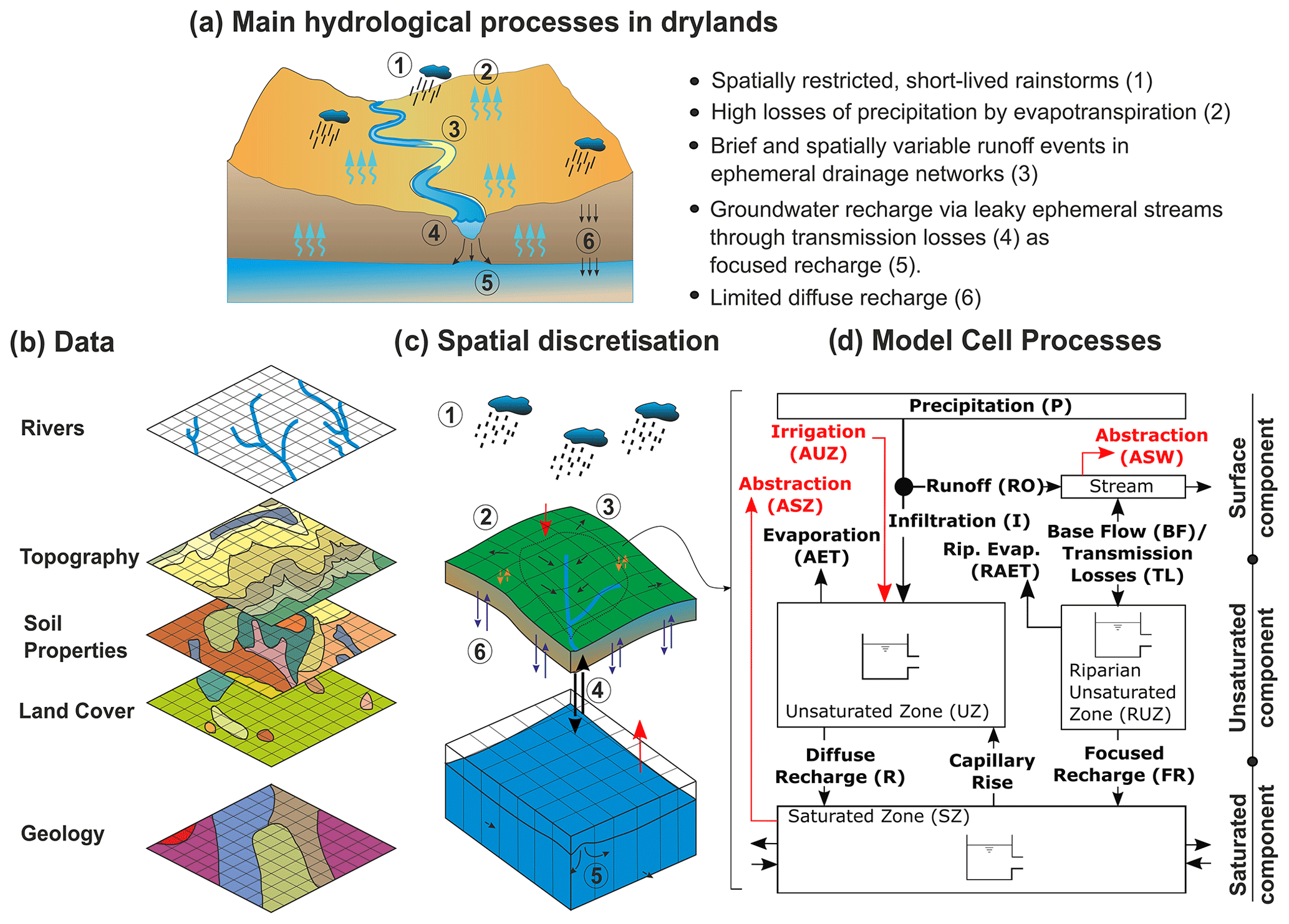
Figure 1Schematic representation of DRYP showing (a) the main hydrological processes controlling water partitioning in dryland regions; (b) distributed data sets needed to derive input parameters; (c) vertical and horizontal discretisation and representation of topographically driven surface runoff, vertical flow in the unsaturated zone, and hydraulic gradient-driven groundwater flow in the saturated component; and (d) model structure and potential processes within a single grid cell for the surface component (see Sect. 2.2), unsaturated zone (see Sect. 2.3), and saturated zone (see Sect. 2.4). Arrows represent flow directions, and red lines represent anthropogenic fluxes.
The only forcing variables in DRYP are spatially explicit fields of precipitation and potential evapotranspiration. The partitioning of the water balance then depends on the combination of this forcing and its interactions with spatially distributed parameters representing topography, land cover, soil hydraulic properties, hydrogeological characteristics of the aquifer, and anthropogenic activities (Fig. 1b). Hydrological processes in DRYP are structured into three main components: (i) a surface water component (SW) where precipitation is partitioned into infiltration and overland flow, which is then routed through the model domain based on the topographic gradient; (ii) an unsaturated zone (UZ) component that represents the soil and a riparian area parallel to streams; and (iii) a saturated zone (SZ) component that represents groundwater flow (Fig. 1c). All three components in DRYP are discretised as square grid cells, and all components are vertically integrated into a computational one-way sequential scheme (Fig. 1c). However, all components are hydraulically interconnected, allowing for gradient-driven and potentially bidirectional water exchange (Fig. 1c, d).
DRYP is written in Python and uses the Python-based “Landlab” package, which has the versatility to handle gridded data sets and model domains (Hobley et al., 2017; Barnhart et al., 2020). DRYP is structured in a modular way to allow user flexibility to control the desired level of process and parameter complexity, as well as the grid size and time-stepping choices appropriate for the desired application of the model. The grid size is the same for all layers, but the time step for different components may vary flexibly as described below. All grid cells potentially consist of all the process elements shown in Fig. 1d. However, the stream and riparian components can be excluded if stream channel characteristics are not provided, in which case all generated runoff in a cell will simply be routed to the next downstream cell with no additional losses or interactions. The scale of the stream and riparian zone is only limited by the grid size.
For all cells, at the beginning of every time step, the input rainfall (P) is partitioned into surface runoff (RO) and infiltration (I) depending on the available water content of the unsaturated zone (UZ). Water in the UZ can be extracted as actual evapotranspiration (AET), a combination of soil evaporation and plant transpiration, and/or percolate (R) to the saturated zone (SZ), depending on the water content and hydraulic properties of the unsaturated zone. If a cell is defined as a stream, transmission losses (TL) or groundwater discharge contributing to base flow (BF) and a riparian unsaturated zone (RUZ) are included in the local partitioning. The riparian zone is defined as an area parallel to the stream with a specified width. The riparian zone receives contributions from TL and a volume of infiltrated water proportional to the riparian area. Water within the riparian zone can either percolate, becoming focused recharge, or it can be extracted by plants as riparian evapotranspiration. Focused and diffuse recharge are combined as the main inputs to the SZ, which may also interact with the UZ depending on the water table elevation as it rises and falls through the simulation. The movement of water in the SZ is driven by the lateral hydraulic gradient. Additionally, anthropogenic interactions in the model are implemented as localised fluxes from the saturated zone (ASZ) and streams (AOF), whereas water abstraction for irrigation (AUZ) is delivered to the surface where it then contributes to infiltration into the unsaturated zone.
2.2 Model input files and parameter settings
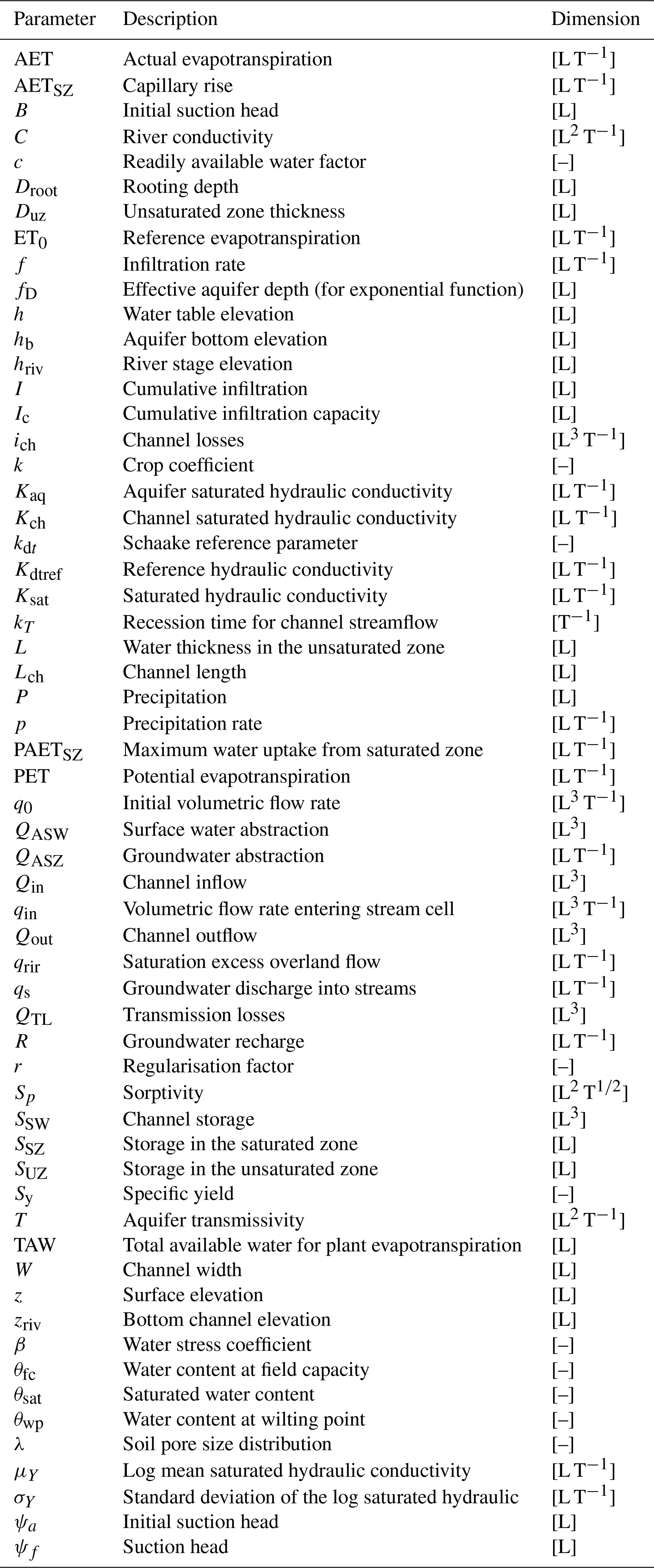
DRYP requires spatial characterisation of key input parameters and data including a digital elevation model (DEM), channel properties in cells where streams are explicitly defined (length, width, and saturated hydraulic conductivity), land cover (plant rooting depth), various soil hydraulic properties, and aquifer properties (specific yield, aquifer thickness, and saturated hydraulic conductivity) (Fig. 1). Where local-scale information is not available for parameterisation, publicly available data at high spatial resolution at the regional and global scales can be considered for model parameterisation (e.g. Pelletier et al., 2016; Leenaars et al., 2018; Dai et al., 2019, etc.). A summary of model parameters for the different model components and structures is presented in Table 1. If parameters are not provided, “global” default values are used as defined in Table 1. The following sections describe the implementation of each process included in DRYP in detail. Precipitation and potential evapotranspiration are the only forcing variables and can be supplied as either spatially variable gridded data sets in netCDF (network common data form) format or as spatially uniform values for each time step. Gridded data sets must be interpolated or aggregated to match the model grid resolution.
Table 1Model parameters for different processes considered in the model; some required parameters depend on the infiltration approach (“Inf. method”). For soil hydraulic properties, default values correspond to a sandy loam soil texture (Clapp and Hornberger, 1978; Rawls et al., 1982).
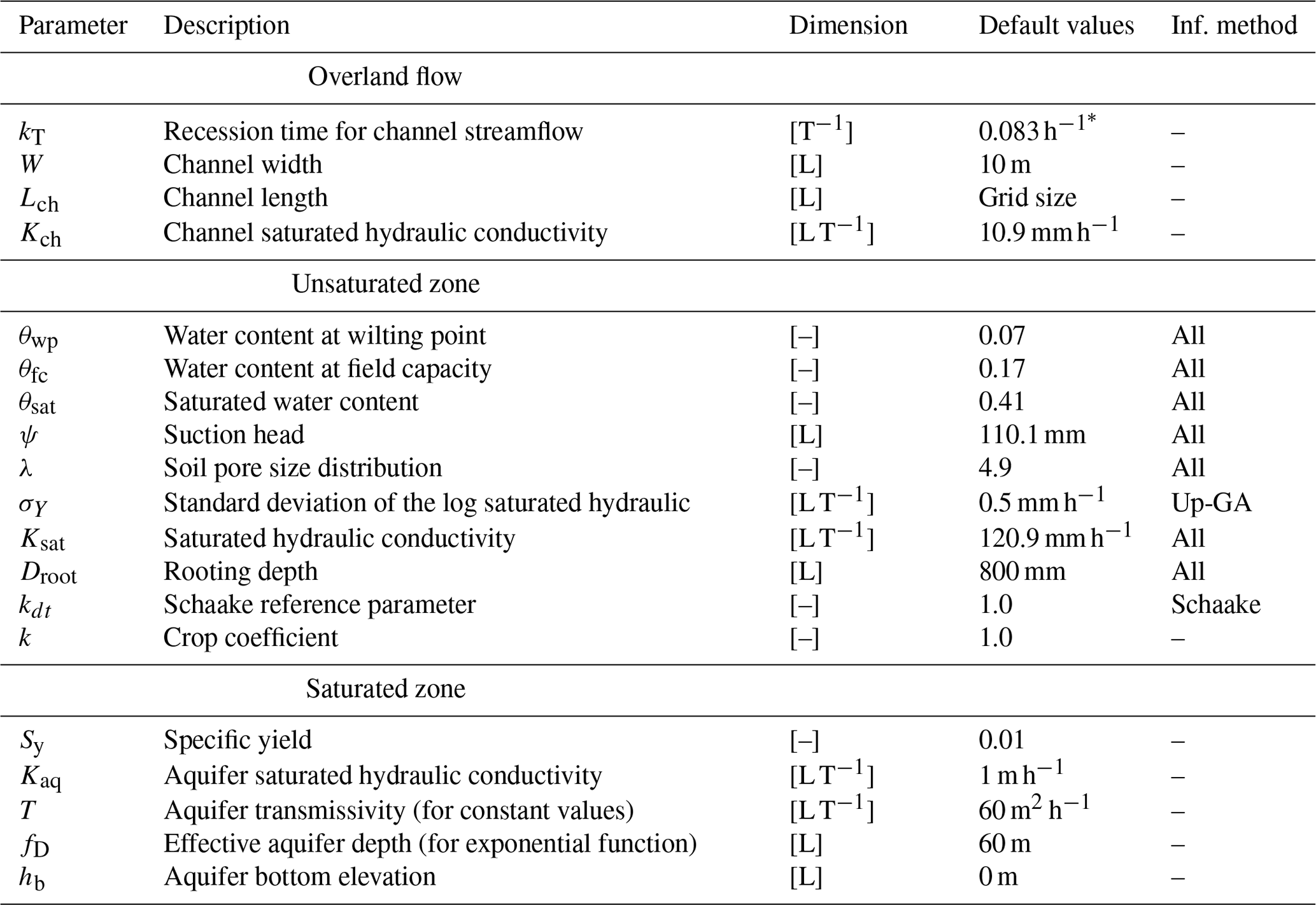
* Default values correspond to a flow velocity of ∼ 1 m s−1 over a 300 m straight path.
2.3 Surface component
Two main processes are considered in the surface component: (i) the partitioning of precipitation into infiltration and runoff, and (ii) runoff routing and the partitioning of runoff into streamflow and transmission losses in stream cells. These are described below.
2.3.1 Infiltration and runoff
The partitioning of precipitation into infiltration and runoff at the land surface is a key process in drylands and a potentially major source of uncertainty in the overall water partitioning for these regions. Hence, four different infiltration approaches have been included in DRYP, which can be toggled on or off within the main control file (prior to simulation) to allow the user to experiment with different infiltration model structures. These approaches include two point-scale methods: the Philip infiltration approach and the modified Green–Ampt method; and two upscaled methods for summarising infiltration over larger areas: the upscaled Green–Ampt and the multi-scale Schaake approach.
Method 1: infiltration based on Philip's equation
In this option, infiltration, f [L T−1] during a rainfall event is based on the explicit solution of the infiltrability depth of Philip's equation (Philip, 1957):
where Ksat is saturated hydraulic conductivity [L T−1], Sp is sorptivity [L2 T], and tc is time since the beginning of the precipitation event [T]. The sorptivity term is estimated using the following equation (Rawls et al., 1982):
where θ is volumetric water content [L3 L−3], θsat is volumetric water content under saturated conditions [L3 L−3], and ψf is suction head [L]. ψf is estimated as follows (Clapp and Hornberger, 1978):
where ψa is maximum suction head [L], and λ is a parameter that represents the pore size distribution of the soil [–] (Clapp and Hornberger, 1978).
The total infiltration depth in any given cell, I [L], during a precipitation event is estimated by solving the integral of Eq. (1) over the event duration. The integral of Eq. (1) is solved using the time compression approach (TCA) (Sherman, 1943; Holtan, 1945; Mein and Larson, 1973; Sivapalan and Milly, 1989), assuming that infiltration after ponding depends on the cumulative infiltrated volume. Therefore, to match the initial infiltration rate at the beginning of each time step with the infiltration at the end of the previous time step, the start time of infiltration is shifted to match the total cumulative infiltration. A more detailed description and the analytical solution of the approach can be found in Assouline (2013) and Chow et al. (1988).
Method 2: infiltration based on a modified Green–Ampt method
We have implemented a modified version of the Green–Ampt approach defined by the following equation (Scoging and Thornes, 1979; Michaelides and Wilson, 2007):
where B represents the initial suction head [L], and tc is the same as Eq. (1); here, we use sorptivity (Eq. 2) as a proxy for the initial head owing to the non-linear dependency of sorptivity on the water content of the soil.
The integral of Eq. (4) was also solved using the time compression approach (Sherman, 1943; Holtan, 1945; Mein and Larson, 1973; Sivapalan and Milly, 1989). However, as there is no explicit solution for Eq. (4), we used an implicit solution.
Method 3: infiltration based on an upscaled Green–Ampt method
This method is based on the semi-analytical solution of the Green–Ampt equation for spatially heterogeneous hydraulic conductivity developed by Craig et al. (2010):
where is the mean infiltration rate [L T−1], p is the precipitation rate [L T−1], tc is the same as in Eq. (1), fk is the probability density function of Ksat, μY and σY are mean and standard deviation of the log saturated hydraulic conductivity, , and X is a dimensionless time. X is estimated as follows:
where , with ψf representing the suction head.
The ε(X,Ks) in Eq. (5) is an error function that can be estimated by the following approximation (Craig et al., 2010):
The fk(Ks) is assumed as a lognormal distribution following Craig et al. (2010):
As suggested by Craig et al. (2010), we solve the integral of the Eq. (5) efficiently using a two-point Gauss–Lagrange numerical integration method.
Method 4: infiltration based on the multi-scale Schaake method
The Schaake et al. (1996) approach is based on the assumption that rainfall and infiltration rates follow an exponential distribution to approximate the spatial heterogeneity of soil properties. Therefore, the spatially averaged infiltration I [L] is estimated as
where P is total rainfall [L], and Ic is cumulative infiltration capacity [L].
Infiltration capacity is estimated as follows (Schaake et al., 1996):
where kdt is a constant that depends on soil hydraulic properties.
Following Chen and Dudhia (2001), we define kdt as
where Kref [L T−1] is a reference hydraulic saturated conductivity equal to m s−1 (Wood et al., 1998; Chen and Dudhia, 2001), and the parameter is specified as a scale calibration parameter.
2.3.2 Runoff routing and transmission losses
Rainfall that does not infiltrate (i.e. precipitation, P, minus infiltration, I) into the unsaturated component is routed over the model domain based on topography. The flow routing scheme varies depending on whether a cell is defined as a stream. A simple flow accumulation approach is used in cells without a defined stream, whereas for defined stream cells, an additional flux term is added to the flow accumulation approach to account for groundwater interactions via the riparian zone. This flux will either be a transmission loss or a base flow contribution from the saturated component.
Flow routing in cells without streams
Runoff produced in any given cell is instantaneously routed to the next downstream cells using the flow accumulation approach implemented in Landlab (Braun and Willett, 2013; Hobley et al., 2017).
The next runoff downstream cell is estimated using a D8 flow direction approach (eight potential directions based on adjacent cells). The flow accumulation method adds the amount of runoff from the upstream cells:
where Qin [L3] is the volume of water that discharges from upstream cells into the current cell i, N is the number of upstream cells discharging into the current cell, and Qi [L3] is the volume of water in the cell.
Flow routing in stream cells
In defined stream cells, the amount of water entering the cell, qin [L3 T−1], is instantly reduced by any transmission losses, ich [L3 T−1], and any remaining water, qout [L3 T−1], is moved to the next downstream cell:
Water from the upstream cell, qin, is assumed to be released to the next cell following a linear reservoir approach:
where kT [T−1] is a recession term that is equal to the inverse of the residence time of the streamflow at each cell, t* represents time [T], and q0 is the initial flow rate of water entering the channel. q0 is estimated as
where QASW [L3] is the volume of water abstracted from the stream, and SSW [L3] is water stored in the channel.
It is assumed that the sediments in the streambed are homogenous. In order to use an explicit approach while also maintaining the simplicity of the model, the channel cross section is assumed to be rectangular. Consequently, the rate of infiltration depends on the wetted perimeter of the channel, and the infiltration rate, ich, at the stream cell is estimated assuming a unit gradient Darcian flow across the wetter perimeter:
where Kch [L T−1] is saturated hydraulic conductivity of the streambed, Lch [L] is channel length for a given cell, W is channel width [L], and y is streamflow stage [L]. If the rate of water entering the stream cell is less than the potential channel infiltration rate, flow to the next downstream cell is set to zero (all water is lost via infiltration) and ich=qin.
Stream stage, y, is estimated by assuming that flow velocity does not change along the channel in any given cell (no flow acceleration). Therefore, the streamflow stage and the volume at any time along the channel are kept constant in any given stream cell. A constant velocity approach assumes that there are no backward effects on the streamflow routing approach. Thus, the stream stage is estimated as the height of the rectangular prism with area A=WLch and volume at time t as follows:
After substituting Eq. (17) into Eq. (16) and then into Eq. (13), the time integral of Eq. (13) represents the total amount of water, Qout [L3], that moves to the next downstream channel cell (becoming Qin):
Note that the time step choice is important to bear in mind with respect to the size of the catchment modelled, as it represents the minimum travel time for flow to reach the catchment outlet.
The amount of water stored in the channel is estimated by applying a mass balance of all inputs and outputs of the channel:
where t represents the current time step, and QTL [L3] is transmission losses estimated as the integral of the second term of Eq. (18). The total of QTL is restricted to the storage available in the aquifer:
where z is the surface elevation [L], h is water table elevation [L], A is the area of cell [L2], and Sy is aquifer specific yield [–].
2.4 Unsaturated component
Water infiltrated into the soil or through the stream channel becomes a flux input to the UZ (Fig. 1d). The unsaturated component comprises the soil and the riparian zone, both of which are simulated using a linear `bucket' soil moisture balance model (Fig. 2a), following an approach similar to the water balance model from the Food and Agriculture Organization (FAO) of the United Nations (Allen et al., 1998):
where ΔS represents storage change [L], AET represents actual evapotranspiration rate [L T−1], and R represents the potential recharge rate [L T−1]. The term QTL is only defined for stream cells. Diffuse potential recharge results from the local vertical percolation of the unsaturated zone, whereas focused potential recharge is produced in the riparian unsaturated zone (see Fig. 1).
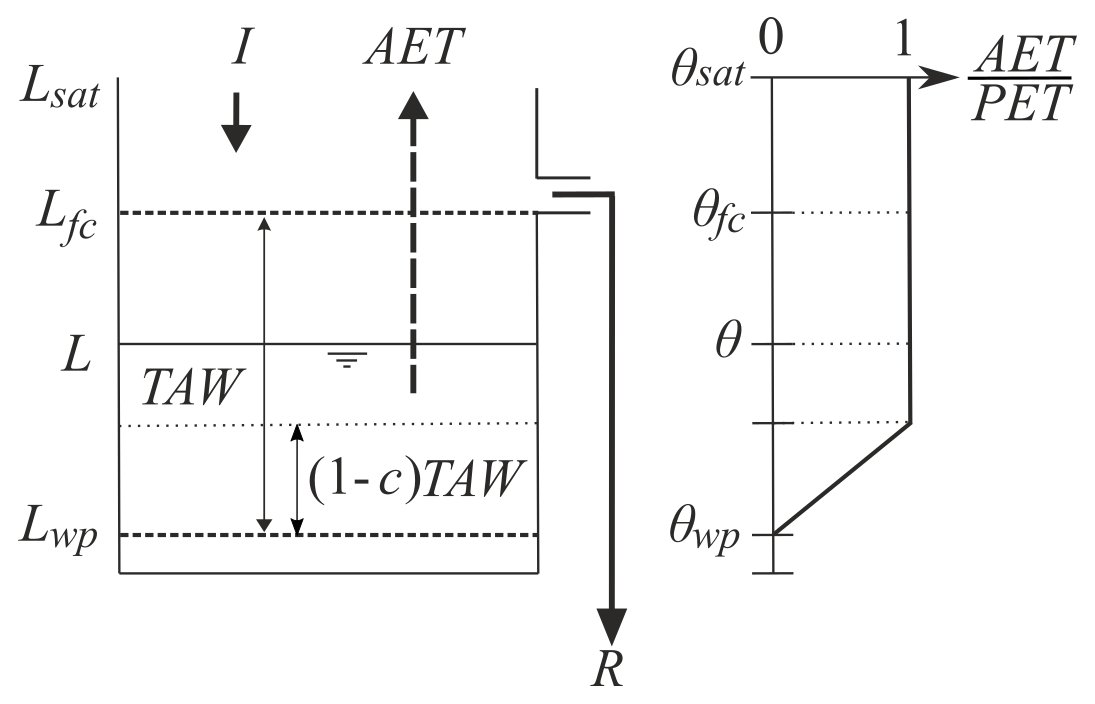
Figure 2Schematic illustration of the unsaturated component. The right panel represents the variation in the ratio of potential to actual evapotranspiration in relation to the water content of the soil. The reader is referred to Sect. 2.3 and 2.4 for a detailed explanation of the terms shown here.
The amount of water available for plant evapotranspiration in the UZ, L [L], is estimated as the product of the rooting depth, Droot [L], and the volumetric water content, θ [L3 L−3]. The maximum amount of water that the soil can store is limited by the field capacity of the soil (Lfc), whereas the minimum amount is constrained by the wilting point (Lwp). Thus, the total available water, LTAW, for plant transpiration is estimated by the difference between Lfc and Lwp (see Fig. 2).
The potential amount of water that plants can remove from the UZ as transpiration, PET [L T−1], is the result of the product between a crop coefficient, k [–], and the reference potential evapotranspiration, ET0 [L T−1] (Allen et al., 1998). When there is enough water to supply plant energy demands, water can be extracted from the UZ at a rate equal to the PET. However, when there is not enough water in the UZ to supply the PET, plants are considered to be under stressed conditions and the actual evapotranspiration (AET) is constrained as
where β is a dimensionless parameter that depends on the water content. β is estimated by
where c is the fraction of LTAW [–] at which plants can extract water from the UZ without suffering water stress; c is set to 0.5, as recommended by the FAO guidelines (Allen et al., 1998), although this can be varied in DRYP.
If, after accounting for infiltration and AET, there is a surplus of water in the soil that exceeds the field capacity, diffuse recharge (R) to the groundwater system occurs. If the model is run at daily time steps, we assume that all water content above field capacity will percolate and produce R. However, for sub-daily time steps, it is more realistic to assume that the soil slowly releases water as R when it is above the field capacity, depending on the soil water retention curve. Hence, in this case, we assume that percolation to the water table depends on the water content and occurs only under the influence of gravity as follows:
where DUZ is the depth of the unsaturated zone [L] (see also Fig. 3a). K(θ) is estimated using the Brooks and Corey (1964) relations and the Clapp and Hornberger (1978) parameters (see Eq. 3):
We then substitute Eq. (25) into Eq. (24) and assume that the soil drains immediately into the groundwater component after evapotranspiration loss. Hence, an analytical solution based only on drainage without considering other inputs or outputs is specified by
The UZ model component in DRYP can also change its behaviour when the head in the SZ component beneath restricts the downward movement of water. This case is described below in Sect. 2.5.1 (unsaturated–saturated zone interactions).
By default, the riparian zone uses the same hydraulic properties of the soil unsaturated zone except for the saturated hydraulic conductivity, which is assumed to be the same as the channel streambed Kch; however, these parameters are also user-defined. The size of the riparian zone has a user-defined width (default is 20 m), and the length is the same as the stream.
2.5 Saturated component
Lateral saturated flow underneath the unsaturated zone assumes the Dupuit–Forchheimer conditions for the Boussinesq equation and Darcian conditions for flow in/out of each model cell:
where Kaq is the saturated hydraulic conductivity of the aquifer [L T−1], Sy is the specific yield [–], qs is saturation excess [L T−1] (see Sect. 2.5.1), qriv is discharge into stream [L T−1] (see Sect. 2.5.2), QASZ [L T−1] is groundwater abstraction, ∇ represents the gradient operator, and ∇⋅ represents the divergence operator. Where the saturated thickness of the aquifer is relatively constant over the simulation period, transmissivity, T [L2 T−1] (the product of the aquifer thickness and the saturated hydraulic conductivity of the aquifer), may be held constant, thereby linearising Eq. (25). Additionally, an exponential function based on Fan et al. (2013) has been added to represent the reduction of transmissivity in relation to depth:
where fD is effective aquifer depth [L]. These different transmissivity parameterisation options can be toggled on or off in the main model control file.
Equation (27) is solved using a forward time central space (FTCS) finite difference approach. FTCS is an explicit finite difference approximation whose solution is sensitive to grid size and time step. Thus, in order to obtain a stable convergence of Eq. (27), a time-variable approach was adopted. The maximum allowable time step for the saturated component is estimated based on the Courant number criteria (we use 0.25 as a default value but this may be changed by the user):
If the maximum time step of the SZ component is greater than the minimum time step of any other component of the model, the time step of the SZ component is reduced to the time step of the minimum time step of the model (see Sect. 2.6 for more details on the model time step options).
2.5.1 Unsaturated–saturated zone interactions
Unsaturated–saturated zone interactions are implemented using a variable-depth unsaturated zone as follows (Fig. 3a). Unsaturated zone thickness (Duz) is equal to the rooting depth when the water table elevation (h) is below the rooting depth, but when the water table is above the rooting depth, the thickness of the unsaturated zone is reduced to the depth of the water table:
When the water table is below the rooting elevation, zroot, there is no two-way interaction between the soil and the groundwater compartment (only one-way, as recharge); thus, no updates to the water table elevation are required (see Fig. 3a1). However, when the water table crosses the zroot threshold, either via recharge or lateral groundwater flow, the water table is updated depending on the change in groundwater storage:
where ΔSSZ is the change in groundwater storage per unit area [L3 L−2]. Specifically, if an SZ cell is being recharged and the water table rises past the rooting depth in a given time step, the water table is updated according to
whereas when the water table is draining and passes the rooting depth in a given time step,
When the water table is above the rooting depth elevation, the water table elevation will be updated according to
whereas if it is below the rooting depth elevation, the water table elevation is simply
When the water table is above zroot, there is more water potentially available for evapotranspiration, as it can be taken from the groundwater reservoir via capillary rise or direct root water uptake. Thus, the potential maximum amount of water taken up from the groundwater reservoir, PAETSZ [L T−1], is computed as the remaining PET after AET from the unsaturated component as follows:
For a shallow water table, upward capillary fluxes may also be taken from the groundwater reservoir. Thus, the rate of actual evapotranspiration from the SZ (AETSZ), including both plant water uptake and capillary rise, is estimated as a linear function of the water table depth as follows:
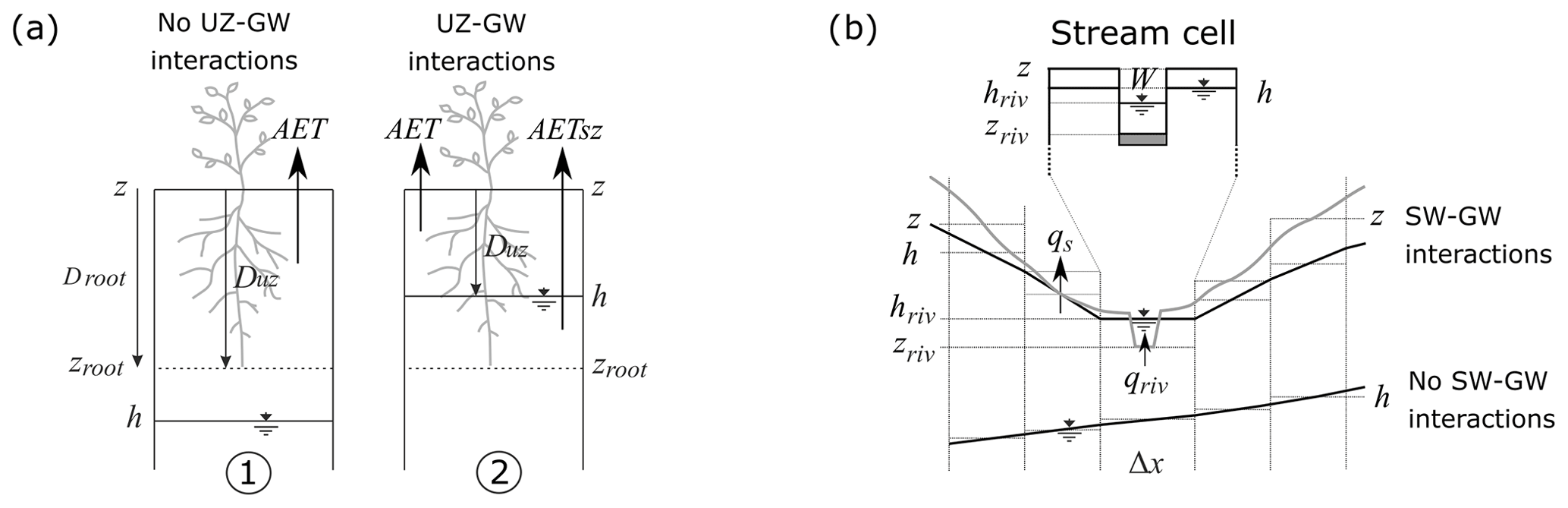
Figure 3Schematic representation of (a) UZ–SZ interactions: (a1) indicates no UZ–SZ interaction, whereas (a2) indicates UZ–SZ interaction (soil depth, Droot, is reduced to Duz). (b) surface water–groundwater (SW–GW) interactions in stream cells: boundary conditions change from no-flow to head-dependent flux conditions once the streambed or ground surface is intersected by the water table. The upper part of panel (b) shows the numerical implementation of SW–GW interactions in a stream cell.
2.5.2 Surface–groundwater interactions
Surface–groundwater interactions are characterised in DRYP through transmission losses, as described in Sect. 2.3.2. In addition, when the water table intersects a cell's defined streambed elevation it produces discharge into the stream, qriv [L T−1], and when the water table reaches the ground surface it produces saturation excess, qs [L T−1] (Fig. 3b) (Eq. 27).
Discharge into streams, qriv, is quantified using a head-dependent flux boundary condition (similar to that used in MODFLOW Harbaugh, 2005):
where C is a conductance term [L2 T−1] estimated as
To avoid numerical instabilities, we use a regularisation approach implemented via a smooth switch between the flux boundary condition and a constant head boundary (and vice versa) using a convex function (Marçais et al., 2017):
where hb is the aquifer bottom elevation [L], and fu is the continuous function between [0, 1]. fu is specified as follows (Marçais et al., 2017):
where r is a dimensionless regularisation factor r > 0, which has been specified as 0.001 following Marçais et al. (2017). fg is the Heaviside step function:
After both qs and qriv are estimated, their corresponding volumes are estimated by multiplying the flow rate, the time step, and the corresponding surface area (cell or stream). The volume is then added as additional runoff in the surface component (Sect. 2.3.2). The water table is updated to its topographical elevation and kept as a constant head boundary condition. The boundary switches back to a flux condition if the water table drops back below the water table.
2.6 Numerical implementation and time step
DRYP is a fully open-source, grid-based model with a layer-based structure, developed using the Landlab architecture (Hobley et al., 2017) and its Python library. Landlab was chosen due to its versatility and modular design, the latter of which allows the user to plug in multiple modules for different levels of complexity and processes using grid-based objects (Hobley et al., 2017; Barnhart et al., 2020).
As most hydrological processes in DRYP, except the SZ component and the modified Green–Ampt infiltration, are described according to explicit analytical solutions, it is possible to run DRYP at hourly or sub-hourly time steps at a low computational cost.
The three main DRYP components (i.e. surface, unsaturated, and saturated components) can run at different time steps, from sub-hourly to daily. The riparian zone of the unsaturated component can also be run at a different time step to that of the unsaturated component. Where different time steps are used between components, the fluxes and state variables are temporally aggregated in DRYP by accumulating and/or averaging them over the specified time step as appropriate and then transferring them to the next component. In addition, and as described above, for the saturated component, an internal time step is also automatically considered to ensure the stability of the numerical solution.
3.1 Evaluation using synthetic experiments
The use of synthetic experiments is an important aspect of model development in hydrology which is welcome but not often used (Clark et al., 2015). The objective of synthetic experiments is to better understand the structural controls on the physical processes represented in the model, for example, on groundwater–soil interactions (Rahman et al., 2019; Batelis et al., 2020). Here, we perform a set of numerical experiments to evaluate the stability and convergence of DRYP components, particularly the coupling of both the surface and unsaturated zone with the groundwater component. Convergence and stability of the numerical solution of the groundwater component using the FTCS finite difference approach and the regularisation have been well documented in different studies (e.g. Wang and Anderson, 1982; Anderson et al., 2015; Marçais et al., 2017). Hence, here we have considered two sets of model evaluations: (i) a quantitative evaluation of the model performance in relation to the well-known numerical model, MODFLOW, for a simple surface–groundwater interaction test represented as a draining condition (see Sect. 3.1.1), and (ii) a qualitative evaluation of the model performance with respect to the desired skill of the model to seamlessly allow interactions between groundwater and the land surface and surface water components (see Sect. 3.1.2).
3.1.1 Comparing DRYP and MODFLOW
For the quantitative evaluation, a 1-D synthetic experiment considering an inclined plane aquifer was set up using DRYP (see Fig. 4a). The length and width of the model domain were specified as 10 and 1 km respectively. Hydraulic saturated conductivity and aquifer specific yield were specified as 1.2 m d−1 and 0.01 respectively. Boundary conditions were specified as no-flow for both the right and left side as well as the bottom of the model domain. The model grid size was set to 1 km × 1 km.
A model with identical geometry, grid size, and hydraulic properties was built in MODFLOW using the “FloPy” Python package (Bakker et al., 2016b, a). Boundary conditions for the MODFLOW model were the same as DRYP except for the top boundary condition, which was specified using the “drain” package (Harbaugh et al., 2000). The elevation at which the water starts to drain was specified as the top surface elevation of the model domain. A high value of the conductivity term (500 m2 d−1) was used in order to capture the seepage process and to ensure convergence as well as minimal water balance errors (Batelaan and Smedt, 2004).
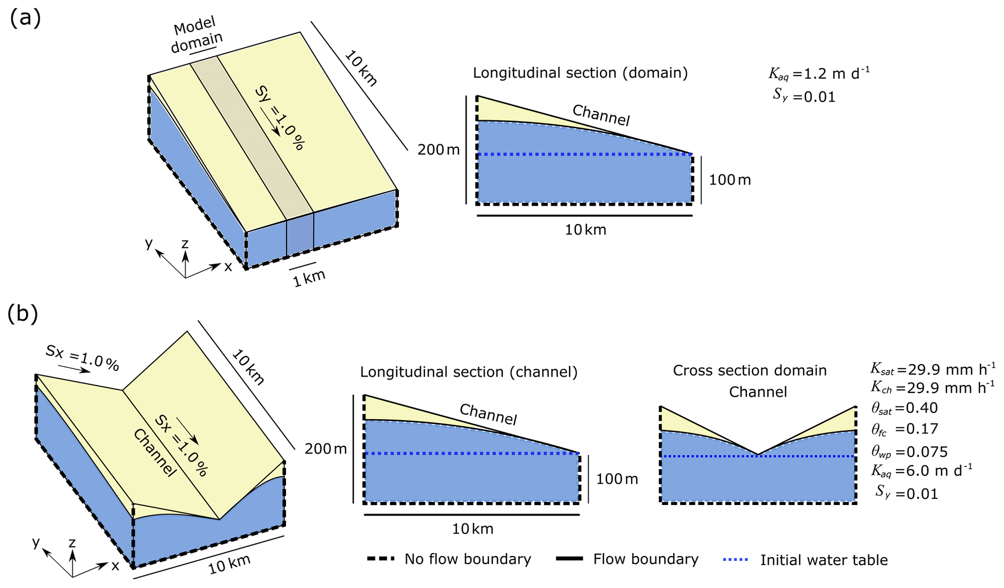
Figure 4Model domain for the synthetic experiments: (a) 1-D model, and (b) tilted-V catchment and flow boundary conditions specified for model simulations.
The synthetic test consisted of a free-draining condition for an unconfined aquifer with a water table depth equal to zero (at the surface level). The time step used for evaluation was 1 d. The evaluation considered the temporal variation in the water table for both DRYP and MODFLOW models, as well as the water balance errors. Errors were evaluated at all locations along the aquifer. Mass balance errors were estimated by the algebraic sum of inputs, outputs, and the storage change.
3.1.2 Qualitative analysis of surface–groundwater interactions
The geometry of the model domain for the qualitative tests consisted of a tilted-V catchment (Fig. 4) with a size of 7×10 square cells on a 1 km resolution grid. Land use and soil hydraulic characteristics were specified as uniform over the entire model domain, and the saturated zone was considered as a homogenous and unconfined aquifer. Boundary conditions were specified as no-flow boundaries for all sides as well as at the bottom of the model domain. The initial water table was set as a horizontal plane at the level of the catchment outlet (100 m) for all simulations (Fig. 4). For experimental purposes, hydraulic characteristics of both the unsaturated and saturated zone were arbitrarily chosen. Thus, a loamy sand soil texture with Ksat= 29.9 cm h−1, θsat= 0.40, θfc= 0.175, and θwp= 0.075 was chosen for the unsaturated zone, whereas, for the saturated zone, the hydraulic conductivity of the aquifer (Kaq) was specified as 6 m d−1, and the specific yield (Sy) was set as 0.01. The high value of Kaq combined with Sy and boundary conditions of the aquifer were applied in order to allow a fast increase/decrease in the water table and the observation of surface–groundwater interaction over a short period of time.
Three main scenarios were analysed using synthetic time series of precipitation and evapotranspiration and changing hydraulic parameters of the UZ:
-
an “infiltration–discharge” scenario, where all precipitation was allowed to infiltrate into the catchment and no infiltration excess was produced over the model domain;
-
an “infiltration–evapotranspiration–discharge” scenario was simulated by adding a time-variable potential evapotranspiration as input into the model;
-
an “infiltration–runoff–evapotranspiration–discharge” scenario was designed to evaluate the production of runoff and focused groundwater recharge, as well as groundwater discharge. For this last scenario, the saturated hydraulic conductivity of the soil was decreased by 1 order of magnitude to produce infiltration excess and, consequently, runoff.
For all three scenarios, precipitation events were specified at a constant value of 0.25 [mm h−1] over 10 d followed by a 20 d dry period. Potential evapotranspiration was specified as a sinusoidal function with a 24 h period and a maximum rate of 0.10 [mm h−1]. These experimental values of precipitation and evapotranspiration combined with the hydraulic properties of the unsaturated and saturated zone allowed a visual evaluation of surface–groundwater interactions under different conditions, such as increasing and decreasing water table through the model run and its interaction with the unsaturated zone.
3.2 Model evaluation based on observed catchment data at Walnut Gulch, USA
In addition to evaluating the DRYP model with synthetic experiments, the model was also evaluated at the Walnut Gulch Experimental Watershed (WGEW), a 149 km2 basin near Tombstone, Arizona, USA (31∘43′ N, 110∘41′ W) (Fig. 5). The climate of the region is semi-arid with low annual rainfall: long-term average of 312 mm yr−1 (Goodrich et al., 2008). The ephemeral channels of WGEW are comprised of mixed sedimentary beds that promote high transmission losses, leading to downstream declining discharge in all but the largest streamflow events (Singer and Michaelides, 2014; Michaelides et al., 2018). WGEW was chosen because it has a long and spatially explicit record of runoff (Stone et al., 2008) for multiple flumes as well as high-density event-based rainfall data for 95 operational gauging stations (Goodrich et al., 2008) which were used to analyse trends in rainfall characteristics (Singer and Michaelides, 2017) and from which the STORM model was created (Singer et al., 2018). In addition, water content from a cosmic-ray neutron sensor as well as latent heat flux from an eddy-covariance flux tower are also available in the basin (Emmerich and Verdugo, 2008; Zreda et al., 2012). Together, these data provide an ideal opportunity to assess many components of a model of dryland water balance and partitioning (Emmerich and Verdugo, 2008; Goodrich et al., 2008; Keefer et al., 2008; Stone et al., 2008; Scott et al., 2015). The water table at WGEW is deep (∼ 50 m at the catchment outlet), so the potential interaction between surface and groundwater is generally unidirectional (Quichimbo et al., 2020).
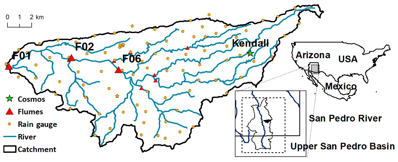
Figure 5Geographic location of the Walnut Gulch Experimental Watershed and the location of monitoring stations.
3.2.1 Model setting, inputs, and parameters
For WGEW, model simulations were performed using the modified Green–Ampt infiltration approach because of its ability to describe the high potential infiltration rates at the beginning of the precipitation event, which are particularly important in this setting. The time step of both the surface component and unsaturated component was specified as 1 h, whereas we use a time step of 1 d for the riparian zone to reduce computational time. The high temporal resolution for the unsaturated component was used to capture the observed high-intensity, low-duration rainfall at WGEW, as well as the influence of diurnal fluctuations in evapotranspiration. As the water table is deep below the ground surface and surface water–groundwater interactions are known to be limited, the groundwater component was not included in model simulations for WGEW.
Spatial and temporal information required as inputs and for model parameters were obtained for WGEW from https://www.tucson.ars.ag.gov/dap/ (last access: 15 October 2021). A model domain of 104×41 square cells on a 300 m resolution grid was developed. A digital elevation model with a spatial resolution of 30 m×30 m was obtained from the Shuttle Radar Topography Mission (SRTM) 1 Arc-Second Global map (available at https://earthexplorer.usgs.gov, last access: 15 May 2021). The DEM was aggregated by averaging cells to the 300 m grid size. Textural characteristics of soil and land cover, obtained as polygon files from https://www.tucson.ars.ag.gov/dap/ (last access: 10 October 2021), were converted into model gridded inputs by considering the feature with the biggest area as the raster value. Based on the soil texture, baseline hydraulic properties required for modelling were obtained from Rawls et al. (1982) and Clapp and Hornberger (1978). Values of field capacity and wilting point required to estimate LTAW (Fig. 2a) were obtained assuming a matric potential of −33 and −1500 kPa following the FAO guidelines (Walker, 1989).
Stream positions were estimated from the 30 m×30 m DEM. The routing network at the 30 m×30 m grid resolution was specified by defining a minimal upstream drainage area threshold of 65 ha, which corresponds to the medium stream network resolution specified in Heilman et al. (2008). Stream cells were then aggregated to the model grid size, 300 m × 300 m, to obtain the stream length at any given cell. Stream width was assumed to be 10 m for the whole model domain based on average values observed across the whole catchment (Miller et al., 2000). Point measurements of rainfall were obtained from 95 rainfall stations that are well distributed within the basin (Goodrich et al., 2008). Rainfall data, at every location, were temporally aggregated to 1 h and then spatially interpolated using a natural neighbour algorithm to a 30 m ×30 m grid size to preserve the high spatial and temporal variability of stations located at distances smaller than the model grid size. Finally, rainfall was spatially aggregated to the grid size of the model domain. Potential evapotranspiration (PET) was calculated using hourly data from the ERA5-Land reanalysis (Hersbach et al., 2020) because this data set enabled high temporal resolution (1 h) and has the potential to drive hydrological and land surface models (Albergel et al., 2018; Alfieri et al., 2020; Tarek et al., 2020; Singer et al., 2021). Data from ERA5 have a spatial resolution of ∼ 9 km at the Equator. The Penman–Monteith approach was chosen to estimate hourly PET due to its high accuracy with respect to producing evapotranspiration values under different climates and locations, and also because it is considered a standard method by the FAO (Allen et al., 1998).
High-resolution temporal measurements of runoff at three flumes (F01, F02, and F06) along the main Walnut Gulch channel were used in the evaluation of runoff generation (Fig. 5). To evaluate modelled soil moisture, we used data from a cosmic-ray neutron sensor station from the COSMOS network (Zreda et al., 2012), located within the Kendall subcatchment of WGEW (Fig. 5). The raw data (publicly available at http://cosmos.hwr.arizona.edu/Probes/StationDat/010/index.php, last access: 20 June 2021) were corrected for atmospheric pressure (Desilets et al., 2010), atmospheric vapour pressure (Rosolem et al., 2013), above-ground biomass, and variation in background intensity using the standardised data processing Cosmic-Ray Sensor PYthon tool (Power et al., 2021) for the period between mid-2010 and 2018.
Finally, data from the AmeriFlux site Kendall Grassland (US-Wkg; available at https://ameriflux.lbl.gov/sites/siteinfo/US-Wkg, last access: 20 June 2021), were used for the evaluation of simulated AET (Fig. 5). Uncertainty in flux tower data is mainly attributed to instrumental and random errors, and it increases with flux magnitude (Richardson et al., 2006; Schmidt et al., 2012). Mean relative errors for AmeriFlux sites are around −5 % with deviations of ±16 % (Schmidt et al., 2012). Historical records from mid-2006 to 2018 were available for model evaluation.
3.2.2 Model sensitivity analysis and calibration
An initial trial-and-error calibration of the model was performed to explore the parameter sensitivities of DRYP and to reduce the a priori parameter ranges used in the second step. This first trial-and-error calibration considered only the performance of the model to represent streamflow at the catchment outlet (flume F01). The calibration was performed by applying spatially constant multiplicative factors kW, kKsat, kDroot, kKch, and kkT, to model parameters W, Ksat, Droot, Kch, and kT respectively. These parameters were used because they control the storage and the water partitioning of components (surface and subsurface components) in the DRYP model for WGEW. Parameters W, Kch, and kT were assumed to be uniform over the entire catchment due to the lack of spatial information, whereas the rest of parameters listed in Table 1 vary depending on their mapped spatial distribution. The initial manual calibration enabled a set of parameter ranges to be defined for a Monte Carlo experiment to analyse the multi-parameter uncertainty of the model results. Then, a set of 1000 realisations was implemented for the analysis with parameters randomly generated using a uniform distribution for each parameter.
The Generalized Likelihood Uncertainty Estimation (GLUE) framework (Beven and Binley, 1992) was used as the uncertainty analysis framework. The GLUE framework considers that, owing to the uncertainty in the input data, model structure, and limitations of boundary condition, there are multiple set of parameters that can produce acceptable simulations. To determine which simulations were considered acceptable (i.e. behavioural), we used a combination of two different “goodness of fit” indices: the Nash–Sutcliffe efficiency (NSE) (Nash and Sutcliffe, 1970) and the per cent bias (PBIAS), which are defined as follows:
Here, O represents the observation, is the arithmetic mean of observations, S represents the model simulations, and n is the number of observations.
In order to define behavioural models, a set of thresholds was specified for the three indices. For streamflow, NSE values higher than 0.50 and PBIAS values less than 20 % (i.e. less than 1 % of the total water budget of the study area) were considered as acceptable simulations. For soil moisture and actual evapotranspiration, only NSE values greater than 0.5 were accepted.
In order to combine these measures into a single performance metric, models that did not meet these conditions were assigned a value of 0, whereas the indexes were linearly scaled between 0 and 1 for the rest of the models. Scaling of NSE values was performed according to the following range: 0 for the minimum value (NSE = 0.5) and 1 for the maximum value of NSE which is also 1. For PBIAS, absolute values were scaled by considering the maximum value (PBIAS = 20 %) equal to 0 and the minimum (PBIAS = 0) equal to 1. The combined performance measure was calculated as the product of all indexes considered in the analysis:
where p is the combined performance measure for the ith parameter set, the * signifies scaled values, and k represents the variable considered in the analysis.
For soil moisture, a direct comparison between observations and simulations was not possible due to differences between the representative soil depths of measurements and simulations. Modelled soil moisture represents the water content of the entire soil column specified by the rooting depth, whereas the observed soil moisture represents the water content over a depth-averaged value, which can be characterised by an effective soil depth that depends on the soil moisture itself (Franz et al., 2012). A direct comparison would result in the misrepresentation of high values of observed soil water content by the model due to the attenuation of peak values over larger soil depths. This problem has been solved by using exponential models that need to be calibrated using measurements at different soil depths (e.g. Wagner et al., 1999; Albergel et al., 2008). Therefore, to enable model–data comparisons that capture the variation in both high and low values of soil moisture observations, we scaled observed soil moisture using the following expression:
where * refers to the scaled value, and α is estimated by
The period between 1 January 2007 and 1 January 2018 was the temporal domain for model simulations at WGEW, with a warm-up period of 1 year prior to this period. This period matches the overlapping period of streamflow observations and flux tower observations. Soil moisture was evaluated for a shorter period of available data between 1 October 2010 and 1 January 2018. Additionally, modelled soil moisture for COSMOS site was obtained by spatial averaging the nine cells located around the COSMOS station to match the typical COSMOS footprint diameter (∼ 700 m) (Desilets and Zreda, 2013; Schrön et al., 2017).
4.1 Comparing DRYP to MODFLOW
The modelling results show a good agreement between DRYP and MODFLOW, and both models ran with negligible mass balance errors ( m3 for DRYP, and m3 for MODFLOW) (see Fig. 6). Both the temporal and spatial variations in the MODFLOW model are well captured by DRYP. Differences in water table elevations are in the range of just 0.022 m at the beginning of the simulation when the aquifer starts to drain, and these differences only decrease as the water table decreases (see Fig. 6a). Temporal variation in the groundwater storage for both models shows consistency, with higher values due to high gradients at the beginning of the simulation, decreasing as the water table declines (see Fig. 6b). More fluctuations are observed in the MODFLOW simulations, which can be attributed to the time step used for the simulation, which needs to be reduced in order to smoothly capture the variation in water table depth as the model switches boundary conditions (Eq. 41). DRYP captures this variation smoothly due to the exponential function and by automatically reducing the time step to assure numerical convergence.
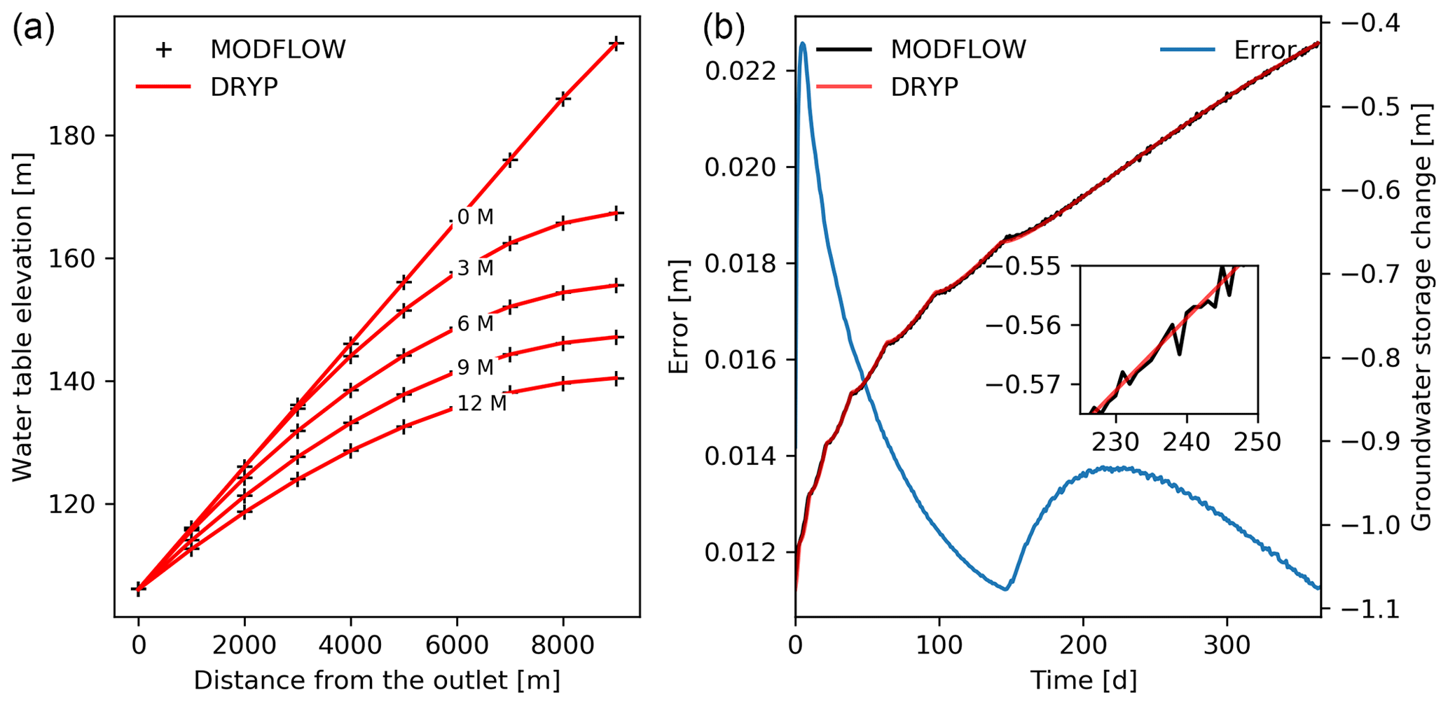
Figure 6(a) Simulated head along the aquifer for different time steps (in months, represented using “M” in panel a) estimated by DRYP (solid lines) and MODFLOW (dashed lines), and (b) temporal variation in the mass balance error for DRYP.
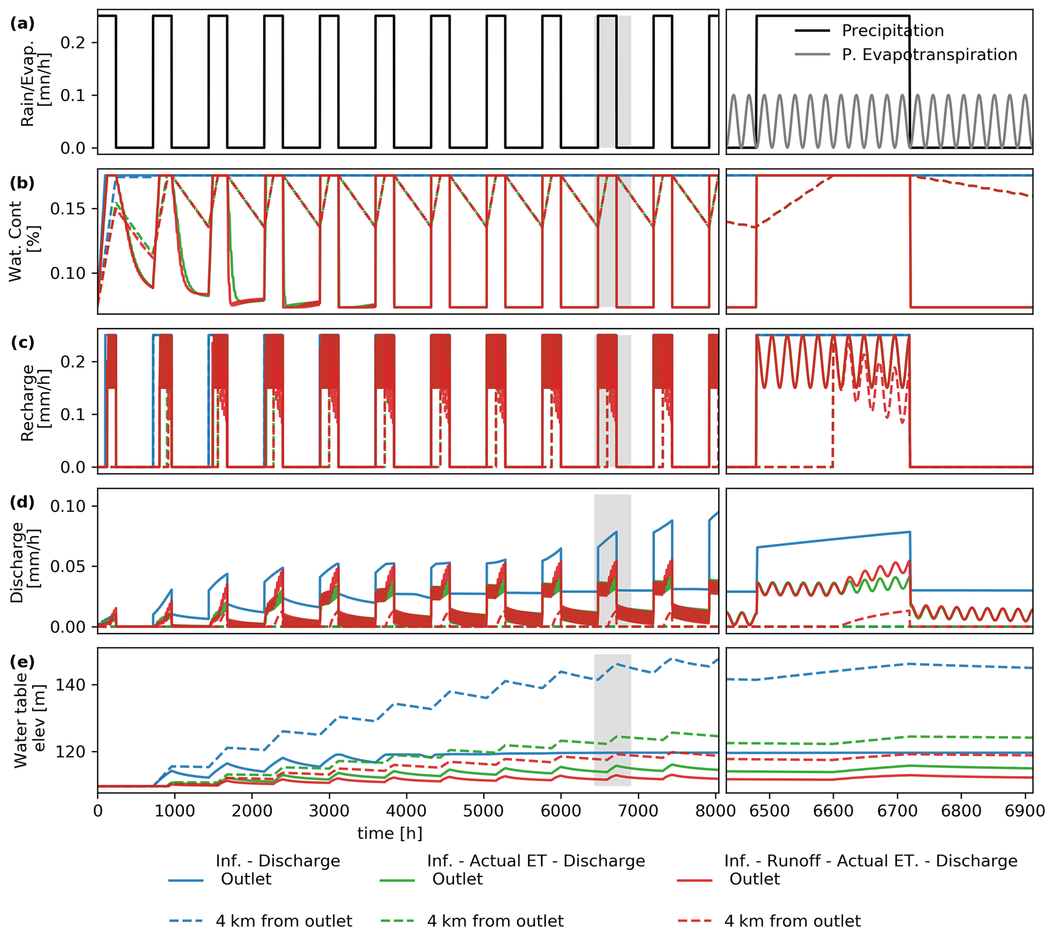
Figure 7Temporal variation in (a) precipitation (black line) and evapotranspiration (grey line), (b) water content of the unsaturated zone, (c) groundwater recharge, (d) runoff/discharge, and (e) water table elevations. The right panels represent zoomed-in sections of the shaded areas in the left panels. Solid lines represent the variation at the catchment outlet, whereas dashed lines represent the temporal variation in the stream at a distance of 4 km from the catchment outlet. For panels (b)–(e), blue lines represent the “infiltration–discharge” scenario, green lines represent the “infiltration–evapotranspiration–discharge” scenario, and red lines represent “infiltration–runoff–evapotranspiration–discharge” scenario.
4.2 Evaluation of qualitative synthetic experiments
Figure 7 shows the temporal variation in fluxes and state variables for the three simulated scenarios at two evaluation points located along the channel, one at the catchment outlet and the second 4 km from the catchment outlet. The respective scenarios' results are described below:
-
In the “infiltration–discharge” scenario (blue lines), precipitation immediately infiltrates into the unsaturated zone when it falls over the catchment (Fig. 6a), increasing the water content of the soil. As there are no losses due to evapotranspiration, the water content steadily increases until it reaches field capacity (Fig. 7b). At field capacity, given that the soil cannot hold any excess water, it starts to release water as diffuse recharge. The soil remains at field capacity for the rest of the simulation, allowing the water from the next rainfall event to move directly to the saturated zone producing recharge (Fig. 7c). Recharge produces an increase in groundwater storage and, consequently, increases the discharge at the outlet of the catchment (Fig. 7d). In the early precipitation events, the contribution of groundwater discharge is minimal. However, this contribution keeps increasing until a dynamic steady state is eventually reached (by 14 600 h, not shown in Fig. 7). Discharge closely follows the temporal variation in the precipitation, due to the high transmissivity of the aquifer and the saturation of the soil; a sharp increase in discharge means that precipitation has become the main contributor to discharge changes because the water table is at the surface (Fig. 7d).
-
In the “infiltration–evapotranspiration–discharge” scenario (green lines), the addition of evapotranspiration in this experiment produces a reduction in soil water content (Fig. 7b). As precipitation is much higher than evapotranspiration, soil moisture quickly reaches a dynamic steady state at the end of the second precipitation event. At cells located close to the catchment outlet, the rise of the water table to ground level reduces the thickness of the unsaturated zone to zero, and as no water can be infiltrated, the soil water content is kept at its highest value during the precipitation event. After the precipitation event, the rate of evapotranspiration, which is greater than the rate of lateral groundwater inflow, gradually reduces the amount of water in the cell. However, as the storage of the SZ keeps increasing, the thickness of the UZ decreases and the rate of lateral groundwater flow becomes greater than the rate of evapotranspiration; this also results in quick changes in the water content of the soil (Fig. 7b). Recharge is also reduced and, as expected, only occurs when the soil moisture reaches field capacity (Fig. 7c). Discharge is also reduced as a result of decreased aquifer recharge due to upward losses by AET. For cells close to saturation, the storage in the groundwater reservoir is affected by evapotranspiration losses (not observed in right panel due to the y axis scale), which in turn results in daily fluctuations in discharge that are the inverse of evapotranspiration fluctuations.
-
In the “infiltration–runoff–evapotranspiration–discharge” scenario (red lines), a reduced Ksat results in the development of infiltration–excess overland flow. The rate of infiltration at the beginning of the precipitation event is high enough to provide water for evapotranspiration without reducing the soil water storage (Fig. 7b), which explains the similarity in soil moisture behaviour with the second scenario. When cells start to produce runoff as a result of infiltration excess, discharge also starts to rise. At stream cells with a deep water table, the increase in streamflow is the result of flow accumulation along the channel during the precipitation event (e.g. Fig. 7d, left panel at 6600 to 6700 h). At cells where the water table interacts with the surface, groundwater discharge gradually increases the streamflow at the catchment outlet at much longer temporal scales (Fig. 7d). At the catchment outlet, streamflow is also affected by the fluctuation of the water table due to the daily variation in evapotranspiration losses (Fig. 7d).
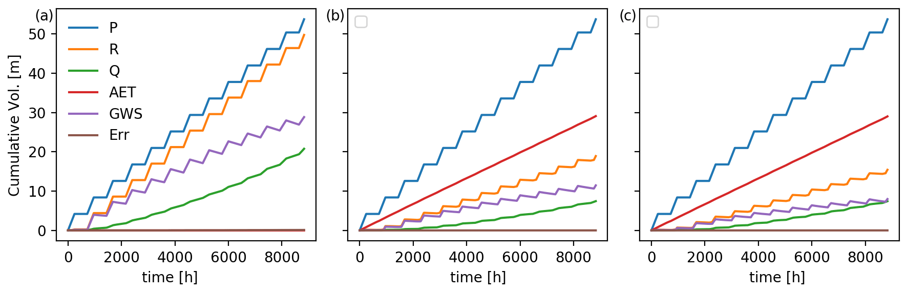
Figure 8Cumulative volume of the main components of the water balance for the simulated scenarios: (a) infiltration–discharge, (b) infiltration–evapotranspiration–discharge, and (c) infiltration–runoff–evapotranspiration–discharge. P is the precipitation, R is recharge, Q is discharge at the catchment outlet, AET is actual evapotranspiration, GWS is the change in groundwater storage, and Err is the water balance error of the simulation.
Figure 8 shows the cumulative volumes of different components of the water balance as well as the cumulative mass balance error of the model. Mass balance errors are low in comparison to the total amount of water entering the catchment, with values of less than 0.12 % for the first case (only precipitation). For the other two cases where evapotranspiration is included, errors are less than 0.02 %. The higher error for the first scenario is attributed to the concentration of flow at the catchment outlet, which leads to an increase in the number of cells discharging into the surface and the channel as well as the resulting minor numerical artefacts.
Coupling of surface and groundwater processes often results in numerical instabilities and in convergence problems (Batelaan and Smedt, 2004; Marçais et al., 2017). However, the results of these synthetic experiments illustrate DRYP's ability to produce realistic hydrological process behaviours by providing a stable solution for representing surface–groundwater interactions without producing numerical artefacts. DRYP is effective at handling the complex coupling and dynamic switching of different types of hydraulic boundary conditions, producing acceptable results with negligible mass balance errors.
4.3 Model performance at WGEW
4.3.1 Spatio-temporal visualisation of the model process simulation at WGEW
The ability of the model to capture the dynamics of dryland hydrological processes is illustrated for WGEW in Fig. 9. The best model (see following section) captures the emergence of ephemeral flow conditions for specific storms, as well as the spatio-temporal changes in soil moisture. It can be seen how, for a given initial soil moisture condition, the production of runoff due to a rainfall event falling over only the central part of catchment results in the concentration of flow along the stream. As water moves downstream, the stream loses water due to transmission losses, which ultimately consumes almost all of the available water by the time runoff reaches the catchment outlet (flume F01 in Fig. 9c).
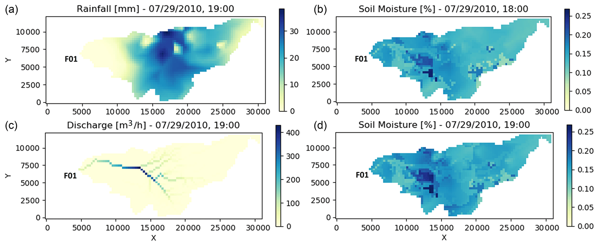
Figure 9Spatio-temporal visualisation of the model process simulation at WGEW: (a) the rainfall event, (b) soil moisture prior to the rainfall event, (c) the ephemeral stream for the rainfall event, and (c) soil moisture after the rainfall event. The x and y axis distance units are in metres.
4.3.2 Characterisation of the temporal variation in simulated variables
Calibration using the trial-and-error method, showed that streamflow displayed particular sensitivity to the parameters Ksat, Droot, Kch, and kT. This informed a set of parameters ranges that were used in the Monte Carlo analysis as follows: for hydraulic conductivity at the channel, kKch, the range varies between 0.10 and 0.30; for kKsat, the range varies between 0.20 and 0.50; for kkT, the range varies between 3 and 10; and for kDroot, the range varies between 0.80 and 1.20. This resulted in 21 behavioural models with values of p above zero. The calibrated parameters for the best simulation were kKch= 0.21, Droot = 1.02, kKsat= 0.30, and kkT= 7.7. A factor of kkT= 7.7 applied to a default value of kT (0.083) represents a flow velocity of 0.41 m s−1 in the channel.
Soil moisture
The DRYP model demonstrates skill at capturing the dynamics of the soil moisture (Fig. 10b) with NSE values of around 0.69. Discrepancies in the magnitude of peak values are likely the result of scaling, so simulations are not able to account for the variation in the effective measurement depth of COSMOS water content estimates (Franz et al., 2012, 2013). The effective COSMOS measurement depth is greater for low values of soil water content (around 33 cm), whereas the effective measurement depth is shallow for higher values of water content (around 16 cm). However, discrepancies may also reflect the limited ability of the soil moisture model to represent high variations occurring at shallow depths of the soil layer, due to the use of a single store.
Evapotranspiration
The DRYP model also skilfully captures (NSE ∼ 0.7) the seasonality and the overall temporal variation in evapotranspiration, a dominant component of the water budget in drylands (Fig. 10c), although peak values are generally overpredicted after long periods of dry conditions. Nevertheless, discrepancies between flux tower data and simulated AET up to 15 % for 1 year have been reported for grassland vegetation in previous studies (Twine et al., 2000; Scott, 2010), and such errors are mainly attributed to the inherent uncertainty in rainfall and latent heat flux measurements (Scott, 2010).
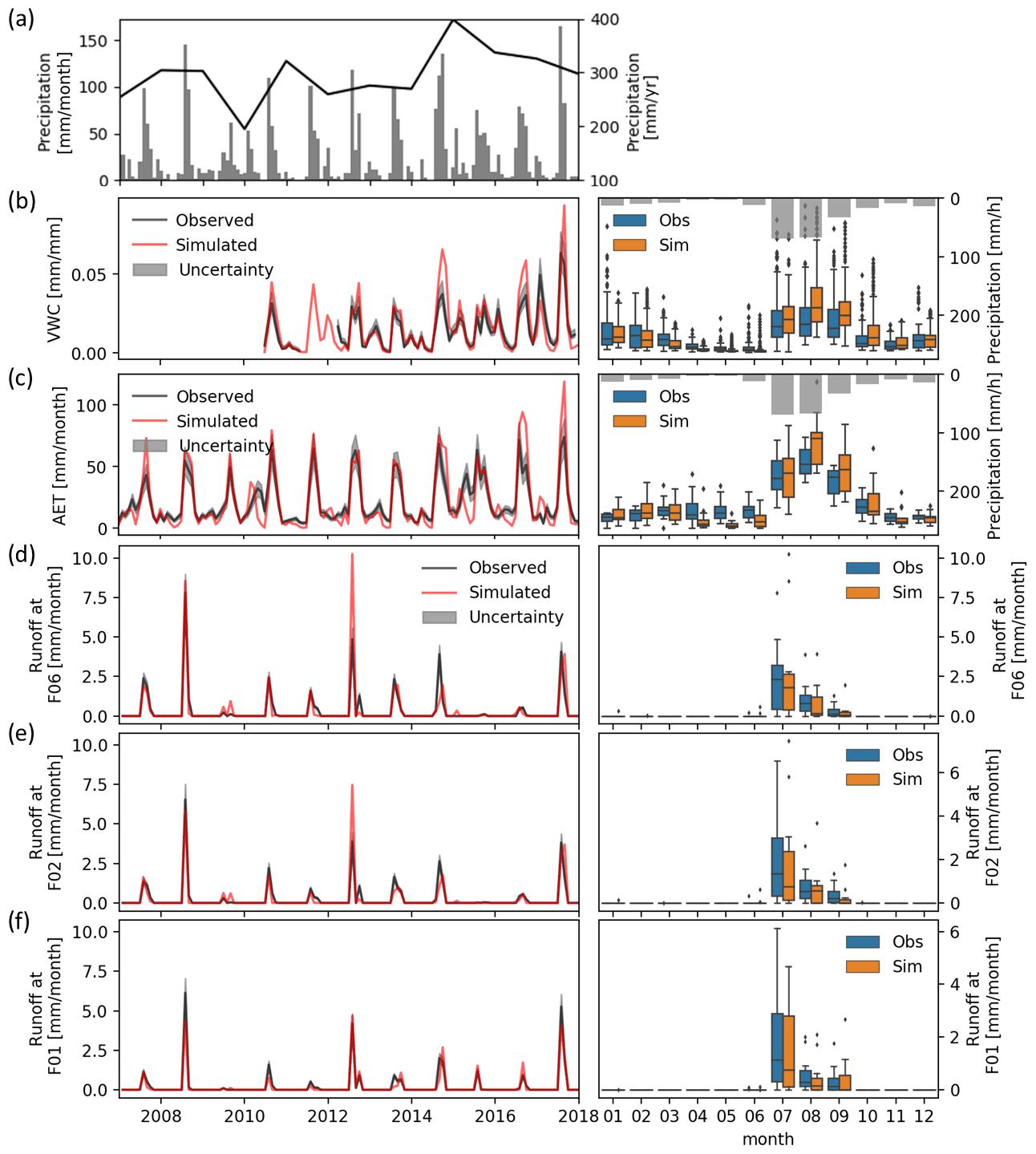
Figure 10Comparison between observed and simulated values of monthly temporal variation (a–f) and monthly distribution (b–f) of (a) monthly precipitation (left axes) and yearly precipitation (right axes), (b) soil moisture at the COSMOS Kendall location, (c) actual evapotranspiration at Kendall, (d) streamflow at flume F06, (e) streamflow at flume F02, and (f) streamflow at flume F01. See Fig. 4 for station locations.
Streamflow
DRYP is also able to reproduce the seasonality and the monthly production of runoff at the outlet of the catchment (F01, NSE ∼ 0.9) (Fig. 10f), as well as at the two upstream flumes (F02, F06) considered in the analysis (NSE > 0.60) (Fig. 10d, e). However, monthly values at flumes F02 and F06 are overpredicted in 2012, perhaps reflecting the development of a crusting layer in previous dry years (e.g. 2009, 2011), a process not included in the model. On the other hand, low production of runoff during wet years (e.g. 2015) may be attributed to the energy of high-intensity rainfall events removing such a crusting layer from the top of the soil, which would result in the increase in infiltration rates (Becker et al., 2018). Additionally, the spatial aggregation of the DEM causes slight inaccuracies in the estimated contributing areas for different streams. This affects not only the volume but also the timing of streamflow events, which may result in over-/underprediction of streamflow events and may ultimately affect the overall water budget.
Water balance
Precipitation shows high annual variability for the evaluated period, with the lowest value of 200 mm yr−1 in 2011 up to 400 mm yr−1 in 2015 (Fig. 10a), which translates into variability in the annual water partitioning for WGEW. For the evaluation period, 1 January 2007 to 1 January 2018, water balance estimates from the best model show that ∼ 92 % of the total precipitation infiltrates into the soil (see Fig. 11). However, almost all infiltrated water returns to the atmosphere as evapotranspiration losses, representing 89 % of the total precipitation. A small proportion, ∼ 3 % of the total precipitation, remains in the soil and the riparian zone, and this stored water corresponds mainly to wetter years of the simulation period (2014 and 2015). Only a small percentage, less than 0.03 %, percolates as diffuse recharge contributing to groundwater storage. Water that does not infiltrate into the soil (8 % of the precipitation) is routed downstream. However, this amount of water is consistently reduced by transmission losses, representing ∼ 7 % of the precipitation. Water entering the riparian zone via transmission losses is partitioned into evapotranspiration and focused recharge. Evapotranspiration consumes up to 60 % of these transmission losses, representing ∼ 4.5 % of the total precipitation. This is broadly consistent with previous studies showing values of 20 mm yr−1 or 5.5 % to 7 % of the total precipitation (Renard, 1970; Renard et al., 2008). The amount of surface water leaving the catchment represents less than 1.0 % of the total amount of precipitation falling over the catchment. These values highlight the impact of transmission losses on the streamflow and aquifer recharge. The main contributor to the total amount of groundwater recharge is focused recharge (∼ 2.5 % of precipitation).
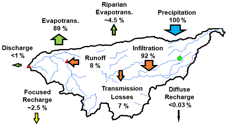
Figure 11Average fluxes of different components of the water budget of WGEW for the simulated period, between 1 January 2007 and 1 January 2018. Water stored in the soil and the riparian zone corresponds to ∼ 3 %. Blue arrows show input fluxes, green arrows represent water leaving the catchment, orange arrows represent internal surface and unsaturated zone fluxes, and yellow arrows represent water moving to the saturated zone (groundwater flow not modelled).
We have developed and presented a parsimonious model to estimate water partitioning in dryland regions (“DRYP”). DRYP is parsimonious in that the model structure has few tunable parameters but still captures the essential elements of dryland hydrology and skilfully represents hydrological stores and fluxes in drylands. It is designed to allow the user to identify mechanisms and factors that affect the water balance in dryland regions, where most existing hydrological models may not be able to capture them appropriately (e.g. the role of focused versus diffuse discharge). We have provided a technical description of all components of DRYP and evaluated it under different scenarios. We first evaluated the ability of DRYP to provide stable numerical simulations of the interaction of surface and subsurface components through synthetic model experiments. We then evaluated DRYP using streamflow, soil moisture, and evapotranspiration data from the semi-arid Walnut Gulch Experimental Watershed (Arizona, USA). We tested the ability of the model to produce behavioural simulations based on multi-parameter Monte Carlo experiments evaluated against a range of objective performance metrics. A comparison between DRYP and MODFLOW for a simple draining-case model showed excellent agreement with an error in hydraulic head of < 0.022 m and a mass balance error of m3. An evaluation of surface–groundwater interactions using numerical experiments over a synthetic model domain indicated that DRYP shows skill at producing stable simulations for the main components of the water balance with low mass balance errors (< 0.12 %). Thus, we conclude that DRYP has the potential to be robustly applied in environments where surface–subsurface interactions play an important role in the overall mass balance of the catchment.
For Walnut Gulch, DRYP effectively captures the spatio-temporal variability of the main components of the dryland water balance at monthly timescales. We find that focused recharge represents ∼ 2.5 % of the total amount of rainfall, whereas diffuse recharge is below 0.03 %. Evapotranspiration is the dominant process representing 90 % of the water leaving the catchment. Evapotranspiration from riparian areas also plays an important role in groundwater recharge, as the amount of water becoming focused recharge is only around ∼ 40 % of the transmission losses.
Considering the combination of explicit solutions of surface and subsurface components, the parsimonious structure, and the low computational cost, it is possible for DRYP to perform long runs using hourly or sub-hourly time steps. These characteristics enable DRYP to test long-term and seasonal changes in water availability to plants and humans in limited-water environments under different scenarios and future climatic conditions such as anthropogenic activities or during droughts. Additionally, given the minimal data requirements, DRYP has the potential to be applied in areas where only information at large scales is available.
Furthermore, improving the soil–vegetation interaction in the unsaturated zone to capture the temporal variation in plant water demand will likely enhance the performance of the model. A more complex representation of the highly dynamic behaviour of ephemeral streamflow will be considered in future developments in order to enhance the ability of the model to represent flooding conditions. Additionally, we also plan to use DRYP in conjunction with stochastic rainfall simulation tools (such as STORM; Singer et al., 2018) to explore the impact of the variability of precipitation on the water balance.
The DRYPv1.0 code is archived at https://doi.org/10.5281/zenodo.5061988 (Quichimbo et al., 2021) and available at https://github.com/AndresQuichimbo/DRYP (last access: 10 October 2021). Our dataset contains modified Copernicus Climate Change Service information (1981–present) available at https://cds.climate.copernicus.eu/cdsapp#!/dataset/reanalysis-era5-single-levels?tab=form (European Centre for Medium-Range Weather Forecasts, 2018). The streamflow dataset used in this research is publicly available at https://www.tucson.ars.ag.gov/dap/runoff_aggregate.asp (Sourthwest Watershed Research Center, 2021). The soil moisture dataset is publicly available at http://cosmos.hwr.arizona.edu/Probes/StationDat/010/index.php (Atmospheric and Geospace Sciences Division of the National Science Foundation, 2021). The flux tower data are publicly available at https://doi.org/10.17190/AMF/1246112 (Scott, 2021).
The supplement related to this article is available online at: https://doi.org/10.5194/gmd-14-6893-2021-supplement.
EAQ, MOC, MBS, KS, and RR conceptualised the study and performed data analysis. EAQ and DH wrote the code. EAQ wrote the original draft of the paper, with further contributions from all co-authors. MOC and MBS provided supervision.
The contact author has declared that neither they nor their co-authors have any competing interests.
Any use of trade, firm, or product names is for descriptive purposes only and does not imply endorsement by Cardiff University.
Publisher's note: Copernicus Publications remains neutral with regard to jurisdictional claims in published maps and institutional affiliations.
The authors would like to thank Ty. P. A. Ferre and the anonymous reviewer for their insightful reviews and comments.
E. Andrés Quichimbo received financial support from Cardiff University through a Vice Chancellor’s Scholarship. Mark O. Cuthbert gratefully acknowledges funding for an Independent Research Fellowship from the UK Natural Environment Research Council (grant no. NE/P017819/1). Michael Bliss Singer has been supported by the U.S. National Science Foundation (grant nos. BCS-1660490 and EAR-1700517) and the U.S. Department of Defense’s Strategic Environmental Research and Development Program (grant no. RC18-1006). Rafael Rosolem has been supported by the Natural Environment Research Council (NERC), under the MOSAIC Digital Environment Feasibility Study (grant no. NE/T005645/1), and by the International Atomic Energy Agency of the United Nations (IAEA/UN; project no. CRP D12014). The team has been supported by the Global Challenges Research Fund (GCRF; “Impacts of Climate Change on the Water Balance in East African Drylands”), The Royal Society (“DRIER”, grant no. CHL\R1\180485), and the European Union's Horizon 2020 programme (“DOWN2EARTH”, grant no. 869550).
This paper was edited by David Lawrence and reviewed by Ty P. A. Ferre and one anonymous referee.
Abbott, M. B., Bathurst, J. C., Cunge, J. A., O'Connell, P. E., and Rasmussen, J.: An introduction to the European Hydrological System – Systeme Hydrologique Europeen, “SHE”, 2: Structure of a physically-based, distributed modelling system, J. Hydrol., 87, 61–77, https://doi.org/10.1016/0022-1694(86)90115-0, 1986.
Abdulrazzak, M. J.: Losses of flood water from alluvial channels, Arid Soil Res. Rehab., 9, 15–24, https://doi.org/10.1080/15324989509385870, 1995.
Albergel, C., Rüdiger, C., Pellarin, T., Calvet, J.-C., Fritz, N., Froissard, F., Suquia, D., Petitpa, A., Piguet, B., and Martin, E.: From near-surface to root-zone soil moisture using an exponential filter: an assessment of the method based on in-situ observations and model simulations, Hydrol. Earth Syst. Sci., 12, 1323–1337, https://doi.org/10.5194/hess-12-1323-2008, 2008.
Albergel, C., Dutra, E., Munier, S., Calvet, J.-C., Munoz-Sabater, J., de Rosnay, P., and Balsamo, G.: ERA-5 and ERA-Interim driven ISBA land surface model simulations: which one performs better?, Hydrol. Earth Syst. Sci., 22, 3515–3532, https://doi.org/10.5194/hess-22-3515-2018, 2018.
Alfieri, L., Lorini, V., Hirpa, F. A., Harrigan, S., Zsoter, E., Prudhomme, C., and Salamon, P.: A global streamflow reanalysis for 1980–2018, J. Hydrol. X, 6, 100049, https://doi.org/10.1016/j.hydroa.2019.100049, 2020.
Allen, R. G., Pereira, L. S., Raes, D., and Smith, M.: Crop evapotranspiration-Guidelines for computing crop water requirements-FAO Irrigation and drainage paper 56, FAO Rome, 300, D05109, 1998.
Anderson, M. P., Woessner, W. W., and Hunt, R. J.: Applied Groundwater Modeling: Simulation of Flow and Advective Transport, Academic Press – Elsevier, the Netherlands, 632 pp., 2015.
Aryal, S. K., Silberstein, R. P., Fu, G., Hodgson, G., Charles, S. P., and McFarlane, D.: Understanding spatio-temporal rainfall-runoff changes in a semi-arid region, Hydrol. Process., 34, 2510–2530, https://doi.org/10.1002/hyp.13744, 2020.
Assouline, S.: Infiltration into soils: Conceptual approaches and solutions, Water Resour. Res., 49, 1755–1772, https://doi.org/10.1002/wrcr.20155, 2013.
Atmospheric and Geospace Sciences Division of the National Science Foundation: Kendall, available at: http://cosmos.hwr.arizona.edu/Probes/StationDat/010/index.php, last access: 20 June 2021.
Bakker, M., Post, V., Langevin, C. D., Hughes, J. D., White, J., Starn, J., and Fienen, M. N.: FloPy: Python package for creating, running, and post-processing MODFLOW-based models, U.S. Geological Survey, https://doi.org/10.5066/F7BK19FH, 2016a.
Bakker, M., Post, V., Langevin, C. D., Hughes, J. D., White, J. T., Starn, J. J., and Fienen, M. N.: Scripting MODFLOW Model Development Using Python and FloPy, Groundwater, 54, 733–739, https://doi.org/10.1111/gwat.12413, 2016b.
Barnhart, K. R., Hutton, E. W. H., Tucker, G. E., Gasparini, N. M., Istanbulluoglu, E., Hobley, D. E. J., Lyons, N. J., Mouchene, M., Nudurupati, S. S., Adams, J. M., and Bandaragoda, C.: Short communication: Landlab v2.0: a software package for Earth surface dynamics, Earth Surf. Dynam., 8, 379–397, https://doi.org/10.5194/esurf-8-379-2020, 2020.
Batelaan, O. and Smedt, F. D.: SEEPAGE, a New MODFLOW DRAIN Package, Groundwater, 42, 576–588, https://doi.org/10.1111/j.1745-6584.2004.tb02626.x, 2004.
Batelis, S.-C., Rahman, M., Kollet, S., Woods, R., and Rosolem, R.: Towards the representation of groundwater in the Joint UK Land Environment Simulator, Hydrol. Process., 34, 2843–2863, https://doi.org/10.1002/hyp.13767, 2020.
Becker, R., Gebremichael, M., and Märker, M.: Impact of soil surface and subsurface properties on soil saturated hydraulic conductivity in the semi-arid Walnut Gulch Experimental Watershed, Arizona, USA, Geoderma, 322, 112–120, https://doi.org/10.1016/j.geoderma.2018.02.023, 2018.
Beven, K. and Binley, A.: The future of distributed models: model calibration and uncertainty prediction, Hydrol. Process., 6, 279–298, 1992.
Braun, J. and Willett, S. D.: A very efficient O(n), implicit and parallel method to solve the stream power equation governing fluvial incision and landscape evolution, Geomorphology, 180–181, 170–179, https://doi.org/10.1016/j.geomorph.2012.10.008, 2013.
Brooks, R. H. and Corey, A. T.: Hydraulic Properties of Porous Media, Hydrology Paper No. 3, Fort Collins, Colorado State University, 40 pp., 1964.
Chen, F. and Dudhia, J.: Coupling an Advanced Land Surface–Hydrology Model with the Penn State–NCAR MM5 Modeling System. Part I: Model Implementation and Sensitivity, Mon. Weather Rev., 129, 569–585, https://doi.org/10.1175/1520-0493(2001)129<0569:CAALSH>2.0.CO;2, 2001.
Cherlet, M., Hutchinson, C., Reynolds, J., Hill, J., Sommer, S., and von Maltitz, G.: World atlas of desertification, Publication Office of the European Union, Luxembourg, 3rd ed., 295 pp., 2018.
Chow, V. T., Maidment, D. R., and Mays, L. W.: Applied Hydrology, McGraw-Hill Companies, Singapore, 588 pp., 1988.
Clapp, R. B. and Hornberger, G. M.: Empirical equations for some soil hydraulic properties, Water Resour. Res., 14, 601–604, https://doi.org/10.1029/WR014i004p00601, 1978.
Clark, M. P., Fan, Y., Lawrence, D. M., Adam, J. C., Bolster, D., Gochis, D. J., Hooper, R. P., Kumar, M., Leung, L. R., Mackay, D. S., Maxwell, R. M., Shen, C., Swenson, S. C., and Zeng, X.: Improving the representation of hydrologic processes in Earth System Models, Water Resour. Res., 51, 5929–5956, https://doi.org/10.1002/2015WR017096, 2015.
Coes, A. L. and Pool, D. R.: Ephemeral-stream channel and basin-floor infiltration and recharge in the Sierra Vista subwatershed of the Upper San Pedro Basin, Southeastern Arizona: Chapter J in Ground-water recharge in the arid and semiarid southwestern United States, Professional Paper 1703, U.S. Geological Survey, 2007.
Craig, J. R., Liu, G., and Soulis, E. D.: Runoff–infiltration partitioning using an upscaled Green–Ampt solution, Hydrol. Process., 24, 2328–2334, https://doi.org/10.1002/hyp.7601, 2010.
Cuthbert, M. O., Acworth, R. I., Andersen, M. S., Larsen, J. R., McCallum, A. M., Rau, G. C., and Tellam, J. H.: Understanding and quantifying focused, indirect groundwater recharge from ephemeral streams using water table fluctuations, Water Resour. Res., 52, 827–840, https://doi.org/10.1002/2015WR017503, 2016.
Cuthbert, M. O., Gleeson, T., Moosdorf, N., Befus, K. M., Schneider, A., Hartmann, J., and Lehner, B.: Global patterns and dynamics of climate–groundwater interactions, Nat. Clim. Change, 9, 137–141, https://doi.org/10.1038/s41558-018-0386-4, 2019a.
Cuthbert, M. O., Taylor, R. G., Favreau, G., Todd, M. C., Shamsudduha, M., Villholth, K. G., MacDonald, A. M., Scanlon, B. R., Kotchoni, D. O. V., Vouillamoz, J.-M., Lawson, F. M. A., Adjomayi, P. A., Kashaigili, J., Seddon, D., Sorensen, J. P. R., Ebrahim, G. Y., Owor, M., Nyenje, P. M., Nazoumou, Y., Goni, I., Ousmane, B. I., Sibanda, T., Ascott, M. J., Macdonald, D. M. J., Agyekum, W., Koussoubé, Y., Wanke, H., Kim, H., Wada, Y., Lo, M.-H., Oki, T., and Kukuric, N.: Observed controls on resilience of groundwater to climate variability in sub-Saharan Africa, Nature, 572, 230–234, https://doi.org/10.1038/s41586-019-1441-7, 2019b.
Dai, Y., Xin, Q., Wei, N., Zhang, Y., Shangguan, W., Yuan, H., Zhang, S., Liu, S., and Lu, X.: A Global High-Resolution Data Set of Soil Hydraulic and Thermal Properties for Land Surface Modeling, J. Adv. Model. Earth Sy., 11, 2996–3023, https://doi.org/10.1029/2019MS001784, 2019.
Datry, T., Bonada, N., and Boulton, A. (Eds.): Intermittent Rivers and Ephemeral Streams, Ecology and Management, Academic Press – Elsevier, the Netherlands, https://doi.org/10.1016/B978-0-12-803835-2.09997-6, 2017.
de Graaf, I. E. M., Sutanudjaja, E. H., van Beek, L. P. H., and Bierkens, M. F. P.: A high-resolution global-scale groundwater model, Hydrol. Earth Syst. Sci., 19, 823–837, https://doi.org/10.5194/hess-19-823-2015, 2015.
Desilets, D. and Zreda, M.: Footprint diameter for a cosmic-ray soil moisture probe: Theory and Monte Carlo simulations, Water Resour. Res., 49, 3566–3575, https://doi.org/10.1002/wrcr.20187, 2013.
Desilets, D., Zreda, M., and Ferré, T. P. A.: Nature’s neutron probe: Land surface hydrology at an elusive scale with cosmic rays, Water Resour. Res., 46, W11505, https://doi.org/10.1029/2009WR008726, 2010.
Emmerich, W. E. and Verdugo, C. L.: Long-term carbon dioxide and water flux database, Walnut Gulch Experimental Watershed, Arizona, United States, Water Resour. Res., 44, W05S09, https://doi.org/10.1029/2006WR005693, 2008.
European Centre for Medium-Range Weather Forecasts: ERA5 hourly data, ECMWF [data set], available at: https://cds.climate.copernicus.eu/cdsapp#!/dataset/reanalysis-era5-single-levels?tab=form (last access: 20 June 2021), 2018.
Ewen, J., Parkin, G., and O'Connell, P. E.: SHETRAN: Distributed River Basin Flow and Transport Modeling System, J. Hydrol. Eng., 5, 250–258, https://doi.org/10.1061/(ASCE)1084-0699(2000)5:3(250), 2000.
Fan, Y., Li, H., and Miguez-Macho, G.: Global Patterns of Groundwater Table Depth, Science, 339, 940–943, https://doi.org/10.1126/science.1229881, 2013.
Franz, T. E., Zreda, M., Ferre, T. P. A., Rosolem, R., Zweck, C., Stillman, S., Zeng, X., and Shuttleworth, W. J.: Measurement depth of the cosmic ray soil moisture probe affected by hydrogen from various sources, Water Resour. Res., 48, W08515, https://doi.org/10.1029/2012WR011871, 2012.
Franz, T. E., Zreda, M., Rosolem, R., and Ferre, T. P. A.: A universal calibration function for determination of soil moisture with cosmic-ray neutrons, Hydrol. Earth Syst. Sci., 17, 453–460, https://doi.org/10.5194/hess-17-453-2013, 2013.
Giordano, M.: Global Groundwater? Issues and Solutions, Annu. Rev. Env. Resour., 34, 153–178, https://doi.org/10.1146/annurev.environ.030308.100251, 2009.
Goodrich, D. C., Lane, L. J., Shillito, R. M., Miller, S. N., Syed, K. H., and Woolhiser, D. A.: Linearity of basin response as a function of scale in a semiarid watershed, Water Resour. Res., 33, 2951–2965, https://doi.org/10.1029/97WR01422, 1997.
Goodrich, D. C., Keefer, T. O., Unkrich, C. L., Nichols, M. H., Osborn, H. B., Stone, J. J., and Smith, J. R.: Long-term precipitation database, Walnut Gulch Experimental Watershed, Arizona, United States, Water Resour. Res., 44, W08515, https://doi.org/10.1029/2006WR005782, 2008.
Goodrich, D. C., Williams, D. G., Unkrich, C. L., Hogan, J. F., Scott, R. L., Hultine, K. R., Pool, D., Goes, A. L., and Miller, S.: Comparison of Methods to Estimate Ephemeral Channel Recharge, Walnut Gulch, San Pedro River Basin, Arizona, in: Groundwater Recharge in a Desert Environment: The Southwestern United States, American Geophysical Union (AGU), 77–99, 2013.
Goodrich, D. C., Kepner, W. G., Levick, L. R., and Wigington, P. J.: Southwestern Intermittent and Ephemeral Stream Connectivity, JAWRA J. Am. Water Resour. Assoc., 54, 400–422, https://doi.org/10.1111/1752-1688.12636, 2018.
Harbaugh, A. W.: MODFLOW-2005, The U.S. Geological Survey Modular Ground-Water Model – the Ground-Water Flow Process, U.S. Geological Survey Techniques and Methods 6-A16, 2005.
Harbaugh, A. W., Banta, E. R., Hill, M. C., and McDonald, M. G.: MODFLOW-2000, The U.S. Geological Survey Modular Ground-Water Model – User Guide to Modularization Concepts and the Ground-Water Flow Process, Geological Survey (U.S.), Denver, CO, https://doi.org/10.3133/ofr200092, 2000-92, 121, 2000.
Heilman, P., Nichols, M. H., Goodrich, D. C., Miller, S. N., and Guertin, D. P.: Geographic information systems database, Walnut Gulch Experimental Watershed, Arizona, United States, Water Resour. Res., 44, W05S11, https://doi.org/10.1029/2006WR005777, 2008.
Hersbach, H., Bell, B., Berrisford, P., Hirahara, S., Horányi, A., Muñoz-Sabater, J., Nicolas, J., Peubey, C., Radu, R., Schepers, D., Simmons, A., Soci, C., Abdalla, S., Abellan, X., Balsamo, G., Bechtold, P., Biavati, G., Bidlot, J., Bonavita, M., Chiara, G. D., Dahlgren, P., Dee, D., Diamantakis, M., Dragani, R., Flemming, J., Forbes, R., Fuentes, M., Geer, A., Haimberger, L., Healy, S., Hogan, R. J., Hólm, E., Janisková, M., Keeley, S., Laloyaux, P., Lopez, P., Lupu, C., Radnoti, G., Rosnay, P. de, Rozum, I., Vamborg, F., Villaume, S., and Thépaut, J.-N.: The ERA5 global reanalysis, Q. J. Roy. Meteor. Soc., 146, 1999–2049, https://doi.org/10.1002/qj.3803, 2020.
Hobley, D. E. J., Adams, J. M., Nudurupati, S. S., Hutton, E. W. H., Gasparini, N. M., Istanbulluoglu, E., and Tucker, G. E.: Creative computing with Landlab: an open-source toolkit for building, coupling, and exploring two-dimensional numerical models of Earth-surface dynamics, Earth Surf. Dynam., 5, 21–46, https://doi.org/10.5194/esurf-5-21-2017, 2017.
Holtan, H. N.: Time-condensation in hydrograph-analysis, EOS T. Am. Geophys. Union, 26, 407–413, https://doi.org/10.1029/TR026i003p00407, 1945.
Huang, J., Yu, H., Guan, X., Wang, G., and Guo, R.: Accelerated dryland expansion under climate change, Nat. Clim. Change, 6, nclimate2837, https://doi.org/10.1038/nclimate2837, 2015.
Huang, J., Li, Y., Fu, C., Chen, F., Fu, Q., Dai, A., Shinoda, M., Ma, Z., Guo, W., Li, Z., Zhang, L., Liu, Y., Yu, H., He, Y., Xie, Y., Guan, X., Ji, M., Lin, L., Wang, S., Yan, H., and Wang, G.: Dryland climate change: Recent progress and challenges, Rev. Geophys., 55, 719–778, https://doi.org/10.1002/2016RG000550, 2017.
Hughes, A., Mansour, M., Robins, N., and Peach, D.: Numerical Modelling of Run-off Recharge in a Catchment in the West Bank, MODFLOW More 2006 Manag. Ground-Water Syst. Conf. Proc., 1, 385–389, 2006.
Hughes, D. A.: A simple approach to estimating channel transmission losses in large South African river basins, J. Hydrol., 25, 100619, https://doi.org/10.1016/j.ejrh.2019.100619, 2019.
Ivanov, V. Y., Vivoni, E. R., Bras, R. L., and Entekhabi, D.: Catchment hydrologic response with a fully distributed triangulated irregular network model, Water Resour. Res., 40, W11102, https://doi.org/10.1029/2004WR003218, 2004.
Kampf, S. K. and Burges, S. J.: A framework for classifying and comparing distributed hillslope and catchment hydrologic models, Water Resour. Res., 43, W05423, https://doi.org/10.1029/2006WR005370, 2007.
Keefer, T. O., Moran, M. S., and Paige, G. B.: Long-term meteorological and soil hydrology database, Walnut Gulch, W05S07, https://doi.org/10.1029/2006WR005702, 2008.
Kipkemoi, I., Michaelides, K., Rosolem, R., and Singer, M. B.: Climatic expression of rainfall on soil moisture dynamics in drylands, Hydrol. Earth Syst. Sci. Discuss. [preprint], https://doi.org/10.5194/hess-2021-48, 2021.
Lahmers, T. M., Gupta, H., Castro, C. L., Gochis, D. J., Yates, D., Dugger, A., Goodrich, D., and Hazenberg, P.: Enhancing the Structure of the WRF-Hydro Hydrologic Model for Semiarid Environments, J. Hydrometeorol., 20, 691–714, https://doi.org/10.1175/JHM-D-18-0064.1, 2019.
Leenaars, J. G. B., Claessens, L., Heuvelink, G. B. M., Hengl, T., Ruiperez González, M., van Bussel, L. G. J., Guilpart, N., Yang, H., and Cassman, K. G.: Mapping rootable depth and root zone plant-available water holding capacity of the soil of sub-Saharan Africa, Geoderma, 324, 18–36, https://doi.org/10.1016/j.geoderma.2018.02.046, 2018.
Marçais, J., de Dreuzy, J.-R., and Erhel, J.: Dynamic coupling of subsurface and seepage flows solved within a regularized partition formulation, Adv. Water Resour., 109, 94–105, https://doi.org/10.1016/j.advwatres.2017.09.008, 2017.
Maxwell, R. M. and Condon, L. E.: Connections between groundwater flow and transpiration partitioning, Science, 353, 377–380, https://doi.org/10.1126/science.aaf7891, 2016.
Mayes, M., Caylor, K. K., Singer, M. B., Stella, J. C., Roberts, D., and Nagler, P.: Climate sensitivity of water use by riparian woodlands at landscape scales, Hydrol. Process., 34, 4884–4903, https://doi.org/10.1002/hyp.13942, 2020.
Mein, R. G. and Larson, C. L.: Modeling infiltration during a steady rain, Water Resour. Res., 9, 384–394, https://doi.org/10.1029/WR009i002p00384, 1973.
Messager, M. L., Lehner, B., Cockburn, C., Lamouroux, N., Pella, H., Snelder, T., Tockner, K., Trautmann, T., Watt, C., and Datry, T.: Global prevalence of non-perennial rivers and streams, Nature, 594, 391–397, https://doi.org/10.1038/s41586-021-03565-5, 2021.
Michaelides, K. and Wainwright, J.: Modelling the effects of hillslope–channel coupling on catchment hydrological response, Earth Surf. Proc. Land., 27, 1441–1457, https://doi.org/10.1002/esp.440, 2002.
Michaelides, K. and Wilson, M. D.: Uncertainty in predicted runoff due to patterns of spatially variable infiltration, Water Resour. Res., 43, W02415, https://doi.org/10.1029/2006WR005039, 2007.
Michaelides, K., Hollings, R., Singer, M. B., Nichols, M. H., and Nearing, M. A.: Spatial and temporal analysis of hillslope–channel coupling and implications for the longitudinal profile in a dryland basin, Earth Surf. Proc. Land., 43, 1608–1621, https://doi.org/10.1002/esp.4340, 2018.
Miller, S. N., Youberg, A., Guertin, D. P., and Goodrich, D. C.: Channel morphology investigations using Geographic Information Systems and field research, in: Land Stewardship in the 21st Century: The Contributions of Watershed Management, Tucson, Arizona, 13–16 March 2000, 415–419, 2000.
Mudd, S. M.: Investigation of the hydrodynamics of flash floods in ephemeral channels: Scaling analysis and simulation using a shock-capturing flow model incorporating the effects of transmission losses, J. Hydrol., 324, 65–79, https://doi.org/10.1016/j.jhydrol.2005.09.012, 2006.
Nash, I. E. and Sutcliffe, I. V.: River flow forecasting through conceptual models, J. Hydrol., 10, 282–290, 1970.
Noorduijn, S. L., Shanafield, M., Trigg, M. A., Harrington, G. A., Cook, P. G., and Peeters, L.: Estimating seepage flux from ephemeral stream channels using surface water and groundwater level data, Water Resour. Res., 50, 1474–1489, https://doi.org/10.1002/2012WR013424, 2014.
Pelletier, J. D., Broxton, P. D., Hazenberg, P., Zeng, X., Troch, P. A., Niu, G.-Y., Williams, Z., Brunke, M. A., and Gochis, D.: A gridded global data set of soil, intact regolith, and sedimentary deposit thicknesses for regional and global land surface modeling, J. Adv. Model. Earth Sy., 8, 41–65, https://doi.org/10.1002/2015MS000526, 2016.
Philip, J. R.: Theory of Infiltration: The infiltration equation and its solutions, Soil Sci., 171, S34–S46, 1957.
Pilgrim, D. H., Chapman, T. G., and Doran, D. G.: Problems of rainfall-runoff modelling in arid and semiarid regions, Hydrolog. Sci. J., 33, 379–400, https://doi.org/10.1080/02626668809491261, 1988.
Power, D., Rico-Ramirez, M. A., Desilets, S., Desilets, D., and Rosolem, R.: Cosmic-Ray neutron Sensor PYthon tool (crspy): An open-source tool for the processing of cosmic-ray neutron and soil moisture data, Geosci. Model Dev. Discuss. [preprint], https://doi.org/10.5194/gmd-2021-77, in review, 2021.
Quichimbo, E. A., Singer, M. B., and Cuthbert, M. O.: Characterising groundwater–surface water interactions in idealised ephemeral stream systems, Hydrol. Process., 34, 3792–3806, https://doi.org/10.1002/hyp.13847, 2020.
Quichimbo, E. A., Cuthbert, M. O., Singer, M. B., Michaelides, K., Rosolem, R., and Hobley, D. E. J.: DRYP 1.0: A parsimonious hydrological model of DRYland Partitioning of the water balance, In DRYP 1.0: A parsimonious hydrological model of DRYland Partitioning of the water balance (1.0), Zenodo, https://doi.org/10.5281/zenodo.5061988, 2021.
Rahman, M., Rosolem, R., Kollet, S. J., and Wagener, T.: Towards a computationally efficient free-surface groundwater flow boundary condition for large-scale hydrological modelling, Adv. Water Resour., 123, 225–233, https://doi.org/10.1016/j.advwatres.2018.11.015, 2019.
Rawls, W. J., Brakensiek, D. L., and Saxtonn, K. E.: Estimation of Soil Water Properties, T. ASAE, 25, 1316–1320, https://doi.org/10.13031/2013.33720, 1982.
Reinecke, R., Foglia, L., Mehl, S., Trautmann, T., Cáceres, D., and Döll, P.: Challenges in developing a global gradient-based groundwater model (G3M v1.0) for the integration into a global hydrological model, Geosci. Model Dev., 12, 2401–2418, https://doi.org/10.5194/gmd-12-2401-2019, 2019.
Renard, K. G.: The hydrology of semiarid rangeland watersheds, Rep. ARS-41-162, Agricultural Research Service, United States Department of Agriculture, Washington, D.C., 28 pp., 1970.
Renard, K. G., Nichols, M. H., Woolhiser, D. A., and Osborn, H. B.: A brief background on the U.S. Department of Agriculture Agricultural Research Service Walnut Gulch Experimental Watershed, Water Resour. Res., 44, W05S02, https://doi.org/10.1029/2006WR005691, 2008.
Reynolds, J. F., Smith, D. M. S., Lambin, E. F., Turner, B. L., Mortimore, M., Batterbury, S. P. J., Downing, T. E., Dowlatabadi, H., Fernández, R. J., Herrick, J. E., Huber-Sannwald, E., Jiang, H., Leemans, R., Lynam, T., Maestre, F. T., Ayarza, M., and Walker, B.: Global Desertification: Building a Science for Dryland Development, Science, 316, 847–851, https://doi.org/10.1126/science.1131634, 2007.
Richardson, A. D., Hollinger, D. Y., Burba, G. G., Davis, K. J., Flanagan, L. B., Katul, G. G., William Munger, J., Ricciuto, D. M., Stoy, P. C., Suyker, A. E., Verma, S. B., and Wofsy, S. C.: A multi-site analysis of random error in tower-based measurements of carbon and energy fluxes, Agr. Forest Meteorol., 136, 1–18, https://doi.org/10.1016/j.agrformet.2006.01.007, 2006.
Rosolem, R., Shuttleworth, W. J., Zreda, M., Franz, T. E., Zeng, X., and Kurc, S. A.: The Effect of Atmospheric Water Vapor on Neutron Count in the Cosmic-Ray Soil Moisture Observing System, J. Hydrometeorol., 14, 1659–1671, https://doi.org/10.1175/JHM-D-12-0120.1, 2013.
Schaake, J. C., Koren, V. I., Duan, Q.-Y., Mitchell, K., and Chen, F.: Simple water balance model for estimating runoff at different spatial and temporal scales, J. Geophys. Res.-Atmos., 101, 7461–7475, https://doi.org/10.1029/95JD02892, 1996.
Schmidt, A., Hanson, C., Chan, W. S., and Law, B. E.: Empirical assessment of uncertainties of meteorological parameters and turbulent fluxes in the AmeriFlux network, J. Geophys. Res.-Biogeo., 117, G04014, https://doi.org/10.1029/2012JG002100, 2012.
Schreiner-McGraw, A., Ajami, H., and Vivoni, E. R.: Extreme weather events and transmission losses in arid streams, Environ. Res. Lett., 14, 084002, https://doi.org/10.1088/1748-9326/ab2949, 2019.
Schrön, M., Köhli, M., Scheiffele, L., Iwema, J., Bogena, H. R., Lv, L., Martini, E., Baroni, G., Rosolem, R., Weimar, J., Mai, J., Cuntz, M., Rebmann, C., Oswald, S. E., Dietrich, P., Schmidt, U., and Zacharias, S.: Improving calibration and validation of cosmic-ray neutron sensors in the light of spatial sensitivity, Hydrol. Earth Syst. Sci., 21, 5009–5030, https://doi.org/10.5194/hess-21-5009-2017, 2017.
Scoging, H. M. and Thornes, J. B.: Infiltration characteristics in a semiarid environment, in: The Hydrology of areas of low precipitation, Canberra Symposium, Paris, 1979, International Association of Hydrological Sciences, 128, 159–168, 1979.
Scott, R. L.: Using watershed water balance to evaluate the accuracy of eddy covariance evaporation measurements for three semiarid ecosystems, Agr. Forest Meteorol., 150, 219–225, https://doi.org/10.1016/j.agrformet.2009.11.002, 2010.
Scott, R.: US-Wkg: Walnut Gulch Kendall Grasslands, (2021), AmeriFlux BASE US-Wkg Walnut Gulch Kendall Grasslands, Ver. 17-5, AmeriFlux AMP [data set], https://doi.org/10.17190/AMF/1246112, 2021.
Scott, R. L., Biederman, J. A., Hamerlynck, E. P., and Barron-Gafford, G. A.: The carbon balance pivot point of southwestern U.S. semiarid ecosystems: Insights from the 21st century drought, J. Geophys. Res.-Biogeo., 120, 2612–2624, https://doi.org/10.1002/2015JG003181, 2015.
Shanafield, M. and Cook, P. G.: Transmission losses, infiltration and groundwater recharge through ephemeral and intermittent streambeds: A review of applied methods, J. Hydrol., 511, 518–529, https://doi.org/10.1016/j.jhydrol.2014.01.068, 2014.
Sherman, L. K.: Comparison f-curves derived by the methods of sharp and Holtan and of Sherman and Mayer, EOS T. Am. Geophys. Union, 24, 465–467, https://doi.org/10.1029/TR024i002p00465, 1943.
Siebert, S., Burke, J., Faures, J. M., Frenken, K., Hoogeveen, J., Döll, P., and Portmann, F. T.: Groundwater use for irrigation – a global inventory, Hydrol. Earth Syst. Sci., 14, 1863–1880, https://doi.org/10.5194/hess-14-1863-2010, 2010.
Šimunek, J., Van Genuchten, M. T., and Šejna, M.: The HYDRUS software package for simulating two-and three-dimensional movement of water, heat, and multiple solutes in variably-saturated media, Tech. Man. Version, 1, 241, 2006.
Singer, M. B. and Michaelides, K.: How is topographic simplicity maintained in ephemeral dryland channels?, Geology, 42, 1091–1094, https://doi.org/10.1130/G36267.1, 2014.
Singer, M. B. and Michaelides, K.: Deciphering the expression of climate change within the Lower Colorado River basin by stochastic simulation of convective rainfall, Environ. Res. Lett., 12, 104011, https://doi.org/10.1088/1748-9326/aa8e50, 2017.
Singer, M. B., Michaelides, K., and Hobley, D. E. J.: STORM 1.0: a simple, flexible, and parsimonious stochastic rainfall generator for simulating climate and climate change, Geosci. Model Dev., 11, 3713–3726, https://doi.org/10.5194/gmd-11-3713-2018, 2018.
Singer, M. B., Asfaw, D. T., Rosolem, R., Cuthbert, M. O., Miralles, D. G., MacLeod, D., Quichimbo, E. A., and Michaelides, K.: Hourly potential evapotranspiration at 0.1∘ resolution for the global land surface from 1981-present, Sci. Data, 8, 224, https://doi.org/10.1038/s41597-021-01003-9, 2021.
Sivapalan, M. and Milly, P. C. D.: On the relationship between the time condensation approximation and the flux concentration relation, J. Hydrol., 105, 357–367, https://doi.org/10.1016/0022-1694(89)90113-3, 1989.
Sourthwest Watershed Research Center: Online Data access, available at: https://www.tucson.ars.ag.gov/dap/runoff_aggregate.asp, last access: 20 June 2021.
Stone, J. J., Nichols, M. H., Goodrich, D. C., and Buono, J.: Long-term runoff database, Walnut Gulch Experimental Watershed, Arizona, United States, Water Resour. Res., 44, W05S05, https://doi.org/10.1029/2006WR005733, 2008.
Tarek, M., Brissette, F. P., and Arsenault, R.: Evaluation of the ERA5 reanalysis as a potential reference dataset for hydrological modelling over North America, Hydrol. Earth Syst. Sci., 24, 2527–2544, https://doi.org/10.5194/hess-24-2527-2020, 2020.
Taylor, R. G., Scanlon, B., Döll, P., Rodell, M., Beek, R. van, Wada, Y., Longuevergne, L., Leblanc, M., Famiglietti, J. S., Edmunds, M., Konikow, L., Green, T. R., Chen, J., Taniguchi, M., Bierkens, M. F. P., MacDonald, A., Fan, Y., Maxwell, R. M., Yechieli, Y., Gurdak, J. J., Allen, D. M., Shamsudduha, M., Hiscock, K., Yeh, P. J.-F., Holman, I., and Treidel, H.: Ground water and climate change, Nat. Clim. Change, 3, nclimate1744, https://doi.org/10.1038/nclimate1744, 2012.
Taylor, R. G., Todd, M. C., Kongola, L., Maurice, L., Nahozya, E., Sanga, H., and MacDonald, A. M.: Evidence of the dependence of groundwater resources on extreme rainfall in East Africa, Nat. Clim. Change, 3, 374–378, https://doi.org/10.1038/nclimate1731, 2013.
Twine, T. E., Kustas, W. P., Norman, J. M., Cook, D. R., Houser, P. R., Meyers, T. P., Prueger, J. H., Starks, P. J., and Wesely, M. L.: Correcting eddy-covariance flux underestimates over a grassland, Agr. Forest Meteorol., 103, 279–300, https://doi.org/10.1016/S0168-1923(00)00123-4, 2000.
Vergnes, J.-P., Decharme, B., Alkama, R., Martin, E., Habets, F., and Douville, H.: A Simple Groundwater Scheme for Hydrological and Climate Applications: Description and Offline Evaluation over France, J. Hydrometeorol., 13, 1149–1171, https://doi.org/10.1175/JHM-D-11-0149.1, 2012.
Wagner, W., Lemoine, G., and Rott, H.: A Method for Estimating Soil Moisture from ERS Scatterometer and Soil Data, Remote Sens. Environ., 70, 191–207, https://doi.org/10.1016/S0034-4257(99)00036-X, 1999.
Walker, W. R.: Guidelines for Designing and Evaluating Surface Irrigation Systems, FAO Irrigation and Drainage Paper No. 45, FAO, Rome, 1989.
Wang, H. F. and Anderson, M. P.: Introduction to Groundwater Modeling: Finite Difference and Finite Element Methods, W.H.Freeman & Co Ltd, San Francisco, 237 pp., 1982.
Wang, L., Chen, W., Huang, G., and Zeng, G.: Changes of the transitional climate zone in East Asia: past and future, Clim. Dynam., 49, 1463–1477, https://doi.org/10.1007/s00382-016-3400-4, 2017.
Wheater, H., Sorooshian, S., and Sharma, K. D. (Eds.): Hydrological Modelling in Arid and Semi-Arid Areas, 1 edition, Cambridge University Press, Cambridge, New York, 222 pp., 2007.
White, R. P. and Nackoney, J.: Drylands, People, and Ecosystem Goods and Services, World Resources Institute, Washington, D.C., 58 pp., 2003.
Wood, E. F., Lettenmaier, D. P., Liang, X., Lohmann, D., Boone, A., Chang, S., Chen, F., Dai, Y., Dickinson, R. E., Duan, Q., Ek, M., Gusev, Y. M., Habets, F., Irannejad, P., Koster, R., Mitchel, K. E., Nasonova, O. N., Noilhan, J., Schaake, J., Schlosser, A., Shao, Y., Shmakin, A. B., Verseghy, D., Warrach, K., Wetzel, P., Xue, Y., Yang, Z. L., and Zeng, Q. C.: The project for intercomparison of land-surface parameterization schemes (PILPS) phase 2(c) Red-Arkansas River basin experiment: 1. Experiment description and summary intercomparisons, Global Planet. Change, 19, 115–135, https://doi.org/10.1016/S0921-8181(98)00044-7, 1998.
Woodward, C. S. and Dawson, C. N.: Analysis of Expanded Mixed Finite Element Methods for a Nonlinear Parabolic Equation Modeling Flow into Variably Saturated Porous Media, SIAM J. Numer. Anal. Phila., 37, 701–724, https://doi.org/10.1137/S0036142996311040, 2000.
Woolhiser, D. A., Smith, R., and Goodrich, D. C.: KINEROS: a kinematic runoff and erosion model: documentation and user manual, U.S. Department of Agriculture, Washington, D.C., 77 pp., 1990.
Zimmer, M. A., Kaiser, K. E., Blaszczak, J. R., Zipper, S. C., Hammond, J. C., Fritz, K. M., Costigan, K. H., Hosen, J., Godsey, S. E., Allen, G. H., Kampf, S., Burrows, R. M., Krabbenhoft, C. A., Dodds, W., Hale, R., Olden, J. D., Shanafield, M., DelVecchia, A. G., Ward, A. S., Mims, M. C., Datry, T., Bogan, M. T., Boersma, K. S., Busch, M. H., Jones, C. N., Burgin, A. J., and Allen, D. C.: Zero or not? Causes and consequences of zero-flow stream gage readings, WIREs Water, 7, e1436, https://doi.org/10.1002/wat2.1436, 2020.
Zoccatelli, D., Marra, F., Armon, M., Rinat, Y., Smith, J. A., and Morin, E.: Contrasting rainfall-runoff characteristics of floods in desert and Mediterranean basins, Hydrol. Earth Syst. Sci., 23, 2665–2678, https://doi.org/10.5194/hess-23-2665-2019, 2019.
Zreda, M., Shuttleworth, W. J., Zeng, X., Zweck, C., Desilets, D., Franz, T., and Rosolem, R.: COSMOS: the COsmic-ray Soil Moisture Observing System, Hydrol. Earth Syst. Sci., 16, 4079–4099, https://doi.org/10.5194/hess-16-4079-2012, 2012.