the Creative Commons Attribution 4.0 License.
the Creative Commons Attribution 4.0 License.
 | 04 Nov 2021
dh2loop 1.0: an open-source Python library for automated processing and classification of geological logs
Ranee Joshi
Kavitha Madaiah
Mark Jessell
Mark Lindsay
Guillaume Pirot
A huge amount of legacy drilling data is available in geological survey but cannot be used directly as they are compiled and recorded in an unstructured textual form and using different formats depending on the database structure, company, logging geologist, investigation method, investigated materials and/or drilling campaign. They are subjective and plagued by uncertainty as they are likely to have been conducted by tens to hundreds of geologists, all of whom would have their own personal biases. dh2loop (https://github.com/Loop3D/dh2loop, last access: 30 September 2021) is an open-source Python library for extracting and standardizing geologic drill hole data and exporting them into readily importable interval tables (collar, survey, lithology). In this contribution, we extract, process and classify lithological logs from the Geological Survey of Western Australia (GSWA) Mineral Exploration Reports (WAMEX) database in the Yalgoo–Singleton greenstone belt (YSGB) region. The contribution also addresses the subjective nature and variability of the nomenclature of lithological descriptions within and across different drilling campaigns by using thesauri and fuzzy string matching. For this study case, 86 % of the extracted lithology data is successfully matched to lithologies in the thesauri. Since this process can be tedious, we attempted to test the string matching with the comments, which resulted in a matching rate of 16 % (7870 successfully matched records out of 47 823 records). The standardized lithological data are then classified into multi-level groupings that can be used to systematically upscale and downscale drill hole data inputs for multiscale 3D geological modelling. dh2loop formats legacy data bridging the gap between utilization and maximization of legacy drill hole data and drill hole analysis functionalities available in existing Python libraries (lasio, welly, striplog).
- Article
(1909 KB) - Full-text XML
- BibTeX
- EndNote


Drilling is a process of penetrating through the ground that is capable of extracting information about rocks from various depths below the surface. This is useful for establishing the geology beneath the surface. Drill core or cuttings can be collected, thus providing samples for description, interpretation and analysis. The location of where drilling starts is referred to as the collar. As the drilling progresses, survey orientation measurements are taken to be able to convert the specific depths to exact coordinate locations of the drill core being retrieved. In a hard-rock setting, geological drill core logging is the process whereby the recovered drill core sample is systematically studied to determine the lithology, mineralization, structures and alteration zones of a potential mineral deposit. It is usually performed by geologists who classify a rock unit into a code, based on one or multiple properties such as rock type, alteration intensity and mineralization content. Exploration and mining companies rely on the diverse geoscientific information obtained by drill core logging techniques to target and to build models for prospectivity mapping or mine planning. This work focuses on lithological logs, which are the component of a geological log that refers to the geological information on the dominant rock type in a specific downhole interval. Inevitably, lithological drill core logging is subjective and plagued by uncertainty as all logging geologists have their own personal biases (Lark et al., 2014). The information and level of detail contained in logs are highly dependent on the purpose of the study; this already makes geological logging subjective. This subjectivity is also influenced by the lack of a standard between projects and/or companies combined with the personal biases of the logging geologist. Furthermore, it can be difficult to recognize lithology with confidence and to establish subtle variations or boundaries in apparently homogeneous sequences.
With the advent of the digital age, semi-automated drill core logging techniques such as X-ray diffraction (XRD), X-ray fluorescence spectrometry (XRF) and hyperspectral (HS) imaging have provided higher detail of data collection and other properties such as conductivity, volumetric magnetic susceptibility, density using gamma-ray attenuation and chemical elements during logging (Zhou et al., 2003; Rothwell and Rack, 2006; Ross et al., 2013). This has prompted a shift towards using numerical data rather than depending on traditional geological drill core logging procedures (Culshaw, 2005). Multiple methods have been recently applied to geological drill core logging such as wavelet transform analysis or data mosaic (Arabjamaloei et al., 2011; Hill et al., 2020; Le Vaillant et al., 2017; Hill et al., 2015), an artificial neural network model (Lindsay, 2019; Zhou et al., 2019; Emelyanova et al., 2017), and inversion (Zhu et al., 2019). Relying solely on these semi-automatic methods comes with drawbacks as it excludes some of the subjective interpretations that cannot be replaced. The semi-automatic methods are also poor at describing textural characteristics (foliation, banding, grain size variation). Furthermore, a rich amount of legacy data is collected in the traditional drill core logging method, and disregarding this information limits the dataset.
Legacy data are information collected, compiled and/or stored in the past in many different old or obsolete formats or systems, such as handwritten records, aperture cards, floppy disks, microfiche, transparencies, magnetic tapes and/or newspaper clippings, making it difficult to access and/or process them (Smith et al., 2015). Legacy digital data also suffer from a lack of standardization and inconsistency. In geoscience, these are currently scattered amongst unpublished company reports, departmental reports, publications, petrographic reports, printed plans and maps, aerial photographs, field notebooks, sample ticket books, drill core samples, tenement information, and geospatial data, providing a major impediment to their efficient use. This includes geological drill core logs that are the outcome of most expensive part of mineral exploration campaigns: drilling. This is a valuable information source and a key asset that can be used to add value to geoscientific data for research and exploration, design mapping programs and research questions of interest, more efficiently target remapping and sustainable new discoveries, and provide customers with all existing information at the start of the remapping program. Legacy drilling data should not to be abandoned even though (1) their recovery and translation into a digital format is tedious and (2) they may have lower intrinsic quality than observations made with more modern equipment. Griffin (2015) argues that there is no distinction in principle between legacy data and “new” data, as all of it is data. The intention of recovering legacy data is to (a) upcycle information with integration into modern datasets, (b) use salvaged data for new scientific applications and (c) allow re-use of that information into utility downstream applications (Vearncombe et al., 2017). Furthermore, extracting information from legacy datasets is valuable and relatively low-risk as geoscientific insight is added to a project at little or no cost compared to that of drilling (Vearncombe et al., 2016).
The primary challenge in dealing with geological legacy datasets is that a large amount of important data, information and knowledge are recorded in an unstructured textural form, such as host rock, alteration types, geological setting, ore-controlled factors, geochemical and geophysical anomaly patterns, and location (Wang and Ma, 2019). To acknowledge the ambiguity of “unstructured textual form”, we define it in this paper as “descriptive text that lacks a pre-defined format and/or metadata and thus cannot be readily indexed and mapped into standard database fields”. The geological drill core logging forms and formats also vary depending on the company, logging geologist, investigation method, investigated materials and/or drilling campaign. Natural language processing (NLP), also known as computational linguistics, has been used for information extraction, text classification and automatic text summarization (Otter et al., 2020). NLP applications on legacy data have been demonstrated in the fields of taxonomy (Rivera-Quiroz and Miller, 2019), biomedicine (Liu et al., 2011) and legal services (Jallan et al., 2019). Qiu et al. (2020) proposed an ontology-based methodology to support automated classification of geological reports using word embeddings, geoscience dictionary matching and a bidirectional long short-term memory model (Dic-Att-BiLSTM) that assists in identifying the difference in relevance from a report. Padarian and Fuentes (2019) also introduced the use of domain-specific word embeddings (GeoVec) which are used to automate and reduce subjectivity of geological mapping of drill hole descriptions (Fuentes et al., 2020).
Similarity matching has many applications in natural language processing as it is one of the best techniques for improving retrieval effectiveness (Park et al., 2005). The use of text similarity is beneficial for text categorization (Liu and Guo, 2005) and text summarization (Erkan and Radev, 2004; Lin and Hovy, 2003). It has been used to extract lithostratigraphic markers from drill lithology logs (Schetselaar and Lemieux, 2012). Fuzzy string matching, also known as approximate string matching, is the process of finding strings that approximately match a given pattern (Cohen, 2011; Gonzalez et al., 2017). It has been used in language syntax checker, spell-checking, DNA analysis and detection, spam detection, sport and concert event ticket search (Higgins and Mehta, 2018), text re-use detection (Recasens et al., 2013), and clinical trials (Kumari et al., 2020).
Most of the available Python libraries have been built to process extracted and standardized drill hole data. The most common of these are lasio (https://lasio.readthedocs.io/en/latest/, last access: 30 September 2021), which deals with reading and writing Log ASCII Standard (LAS) files, a drill hole format commonly used in the oil and gas industry, welly (https://github.com/agile-geoscience/welly, last access: 30 September 2021), which deals with loading, processing and analysis of drill holes, and striplog (https://github.com/agile-geoscience/striplog, last access: 30 September 2021), which digitizes, visualizes and archives stratigraphic and lithological data. striplog (Hall and Keppie, 2016) also parses natural language “descriptions”, converting them into structured data via an arbitrary lexicon which allows further querying and analysis on drill hole data. The main limitation of these existing libraries, with respect to legacy data in the mining sector, is that they assume that the data are already standardized and pre-processed.
dh2loop provides the functionality to extract and standardize geologic drill hole data and export them into readily importable interval tables (collar, survey, lithology). It addresses the subjective nature and variability of the nomenclature of lithological descriptions within and across different drilling campaigns by integrating published dictionaries, glossaries and/or thesauri that are built to improve the resolution of poorly defined or highly subjective use of terminology and idiosyncratic logging methods. It is, however, important to highlight that verifying the accuracy and/or correctness of the geological logs being standardized is outside the scope of this tool; thus we assume logging has been conducted to the best of the geologist's ability.
Furthermore, it classifies lithological data into multi-level groupings that can be used to systematically upscale and downscale drill hole data inputs in a multiscale 3D geological model. It also provides drill hole de-surveying (computes the geometry of a drill hole in three-dimensional space) and log correlation functions so that the results can be plotted in 3D and analysed against each other. It also links the gap between utilization and maximization of legacy drill hole data and the drill hole analysis functionalities available in existing Python libraries.
2.1 Conventions and terminologies
This paper involves multiple Python libraries, database tables and fields (Appendix A1). For clarity, the following conventions are used for this paper:
-
Python libraries are written in italics: dh2loop
-
Python functions are written in italics followed by an open and close parenthesis: token_set_ratio()
-
Database tables are written in italic typewriter font:
dhgeology -
Database table fields are written in roman typewriter font:
CollarID -
Workflows are written in bold: Lithology Code workflow
2.2 Data source
The Geological Survey of Western Australia (GSWA) Mineral Exploration Reports Database (WAMEX) contains open-file reports submitted as a compliance to the Sunset Clause, Regulation 96(4) of the Western Australia legislation Mining Regulations 1981. These reports contain valuable exploration information in hard copy (1957–2000), hard copy, and digital format (2000–2007) and digital format (2000–present) (Riganti et al., 2015). The minimum contents of a drilling report comprise a collar file, which describes the geographic coordinates of the collar location (Fig. B1). Additional files may be included, such as a survey file describing the depth, azimuth and inclination measurements for the drilling path; assays, downhole geology and property surveys (e.g. downhole geochemistry, petrophysics) may also be available depending on the company's submission (Riganti et al., 2015). The data in the drilling reports are extracted with spatial attribution and imported to a custom-designed relational database (also called the Mineral Drill hole Database) curated by the GSWA that allows easy retrieval and spatial querying. For simplicity, we will refer to this database as the WAMEX database in this text.
The WAMEX database contains more than 50 years' worth of mineral exploration
drill hole data with more than 2.05 million drill holes, imported from over
1514 companies. Each drill hole is identified by its surface coordinates
and its unique ID (CollarID) in the collar table (Fig. B1). The drill hole 3D geometry is
described in the survey tables (dhsurvey, dhsurveyattr). The lithology along the drill hole is
described as a function of depth in the lithology tables (dhgeology and
dhgeologyattr). However, it is important to emphasize that the drill hole data are of
variable quality and reliability and that no validation has been done. The
necessary amendments and reformatting enabling us to extract and utilize data
from the WAMEX database are part of the functionalities provided by
dh2loop.
2.3 Thesauri
Since most exploration companies have their own nomenclature and systems,
which could also change between drilling campaigns, it is necessary to build
thesauri: dictionaries that list equivalent and related nomenclature (or
synonyms) for different attribute names and values. Synonyms include
terms that share a similar intent, for example, RL (relative level)
terms, whether elevation or relative level, as long as the words record a vertical height. These thesauri are stored as additional tables
in the database. For example, if we are interested in the major lithology in
a specific interval, this information can be tabulated as “Major Rock
Type”, “Lithology_A” or “Main_Geology_Unit” depending on the drill core logging system
used. The resulting thesauri considers change in cases, abbreviations,
the addition of characters, typographical errors and a combination of these.
Although listing out these terms is manual and tedious, it only needs to be
done once and can be re-used and forms the basis for future text matching
and as a training set to automate finding similar terms. This is preferred
over selection based on regular expressions as when parsing these terms,
there are complex patterns in the terms used and inconsistencies in the
way they are written that can be understood by a person with a geological
background but not by a simple regular expression. The complexity of the
regular expression required to catch all the terms of interest means an
optimal expression is difficult, if not impossible, to define and also
tends to be computationally burdensome. dh2loop provides several thesauri that can
easily be updated (if needed) for the following attributes (Appendix A1).
In order to extract the other attributes, we envisage developing other
thesauri, following the same workflow.
-
Drill Hole Collar Elevation Thesaurus: 360 synonyms such as “elevation” and “relative level”.
-
Drill Hole Maximum Depth Thesaurus: 160 synonyms such as “end of hole”, “final depth” and “total depth”.
-
Drill Hole Survey Azimuth Thesaurus: 142 synonyms.
-
Drill Hole Survey Inclination Thesaurus: 8 synonyms such as “dip”.
-
Drill Hole Lithology Thesaurus: 688 synonyms such as “geology”, “Lithology_A”, “Major_Geology_Unit” and “Major_ Rock_Type”.
-
Drill Hole Comments Thesaurus: 434 synonyms such as “description”.
The thesauri created specifically for further processing lithology and comment information are the following:
- 7.
Drill Hole Lithology Codes Thesaurus: it compiles the equivalent lithology for a given lithological code based on the reports submitted to GSWA. This thesaurus is identified by a company ID and report number.
- 8.
Clean-up Dictionary: it is a list of words and non-alphabetic characters that are used as descriptions in the geological logging syntax. This dictionary is used to remove these terms from the
Company_Lithoand/orCommentsfree-text descriptions prior to the fuzzy string matching. The dictionary is composed of terms that describe age, location, structural forms, textures, amount or distribution, minerals, colours, symbols and common phrases, compiled from abbreviations in field and mine geological mapping (Chace, 1956) and the CGI-IUGS (International Union of Geological Sciences Commission for the Management and Application of Geoscience Information) geoscience vocabularies accessible at http://geosciml.org/resource/def/voc/ (last access: 30 September 2021) (Simons et al., 2006; Richard and CGI Interoperability Working Group, 2007; Raymond et al., 2012). - 9.
Lithology Hierarchical Thesaurus: it is a list of 757 rock names (
Detailed_Lithology), their synonyms and a two-level upscale grouping (Lithology_SubgroupandLithology_Group) (Fig. 1). Each row inDetailed_Lithologyrefers to a rock name. Each rock name row lists the standardized terminology first, followed by its synonyms. The two corresponding columns for this row indicated the two-level upscale grouping. Many of theLithology_Subgroupslisted have parent–child relationships e.g. “mafic_fine_grained_ crystalline” is a child of “mafic”. Parents in parent–child relationships are included in their children as catch-all groups to capture free-text descriptions that do not include details that would be captured by only using the child terms alone. In total, 169 of these rock names are compiled from the CGI-IUGS Simple Lithology vocabulary available at http://resource.geosciml.org/classifier/cgi/lithology (last access: 30 September 2021) (Simons et al., 2006; Richard and CGI Interoperability Working Group, 2007; Raymond et al., 2012). The synonyms are obtained from https://mindat.org (last access: 30 September 2021) (Ralph, 2021). The hierarchical classification is inherited from both https://mindat.org (Ralph, 2021) and the British Geological Survey (BGS) Classification Scheme (Gillespie and Styles, 1999; Robertson, 1999; Hallsworth and Knox, 1999; McMillan and Powell, 1999; Rosenbaum et al., 2003). It is important to use multiple libraries to be able to build an exhaustive thesaurus as some libraries are limited by the nomenclature, level of interest, and presence of the lithology or rock group in a geographic area. For example, the BGS classification did not have a comprehensive regolith dictionary. Thus, regolith has been classified using the regolith glossary (Eggleton, 2001).
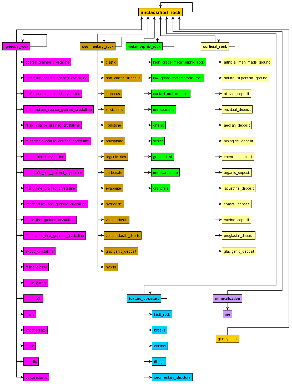
Figure 1Lithology Hierarchical Thesaurus showing the seven major
Lithology_Groups: igneous rocks (pink), sedimentary rocks
(light brown), metamorphic rocks (green), surficial rocks (light yellow),
texture and structure (blue), mineralization (purple) and unclassified rocks
(dark yellow) and their corresponding Lithology_Subgrouups.
2.4 Data extraction
Currently, the dh2loop library extracts collar, survey and lithology information. The paper focuses on the lithological extraction. Database structure and extraction results for collar and survey are available in Appendices B3 and B4. The extraction uses a configuration file that allows the user to define the inputs, which are as follows:
-
region of interest (in WGS (World Geodetic System) 1984 lat/long) and/or
-
list of drill hole ID codes if known
-
if reprojection is desired, the EPSG (European Petroleum Survey Group) code of the projected coordinate system (e.g. EPSG:28350 for MGA (Map Grid of Australia) Zone 50; http://epsg.io, last access: 30 September 2021)
-
the connection credentials to the local copy of the WAMEX database
-
input and output file directories/location.
The lithology extraction is divided into two workflows: Lithology Code workflow and Comments workflow. Both workflows output a lithology CSV file containing the following information (Fig. 2):
-
CompanyID: the primary key to link the lithology code to the Drill Hole Lithology Codes Thesaurus and decode the lithologies. -
CollarID: the primary key to link the lithology information to the collar file. -
FromDepthandToDepth: if theToDepthis null, we assumeToDepthto be equal toFromDepth+ 0.01. If theFromDepthis larger thanToDepth, theFromDepthandToDepthvalues are switched. -
Detailed_Lithology: this value is the lithology matched through fuzzy string matching. The string that serves as input to the fuzzy string matching may either be theCompany_Litho(decoded lithology fromCompany_LithoCode) or from theComments(free-text descriptions).- 4.1.
Decoding Lithological Codes
- 4.1.1.
Company_LithoCode: this fetches the lithology codes that are typically three-letter codes using the Drill Hole Lithology Thesaurus. - 4.1.2.
Company_Litho: theCompany_Lithois fetched by matching theCompanyIDandCompany_LithoCodeto the Drill Hole Lithology Codes Thesaurus.
- 4.1.1.
- 4.2.
Comments: this fetches the free-text descriptions using the Drill Hole Comments Thesaurus.
- 4.1.
-
Lithology_SubgroupandLithology_Group: upscales the lithological information to more generic rock groups. For example,Detailed_Lithology: “basalt” is upscaled toLithology_Subgroup: “mafic_fine-grained crystalline” and further upscaled toLithology_Group: “igneous rock”. -
calculated
X,Y,Zfor the start, mid- and endpoint also using the minimum curvature algorithm. The de-surveying code is heavily based on the pyGSLIB drill hole module.
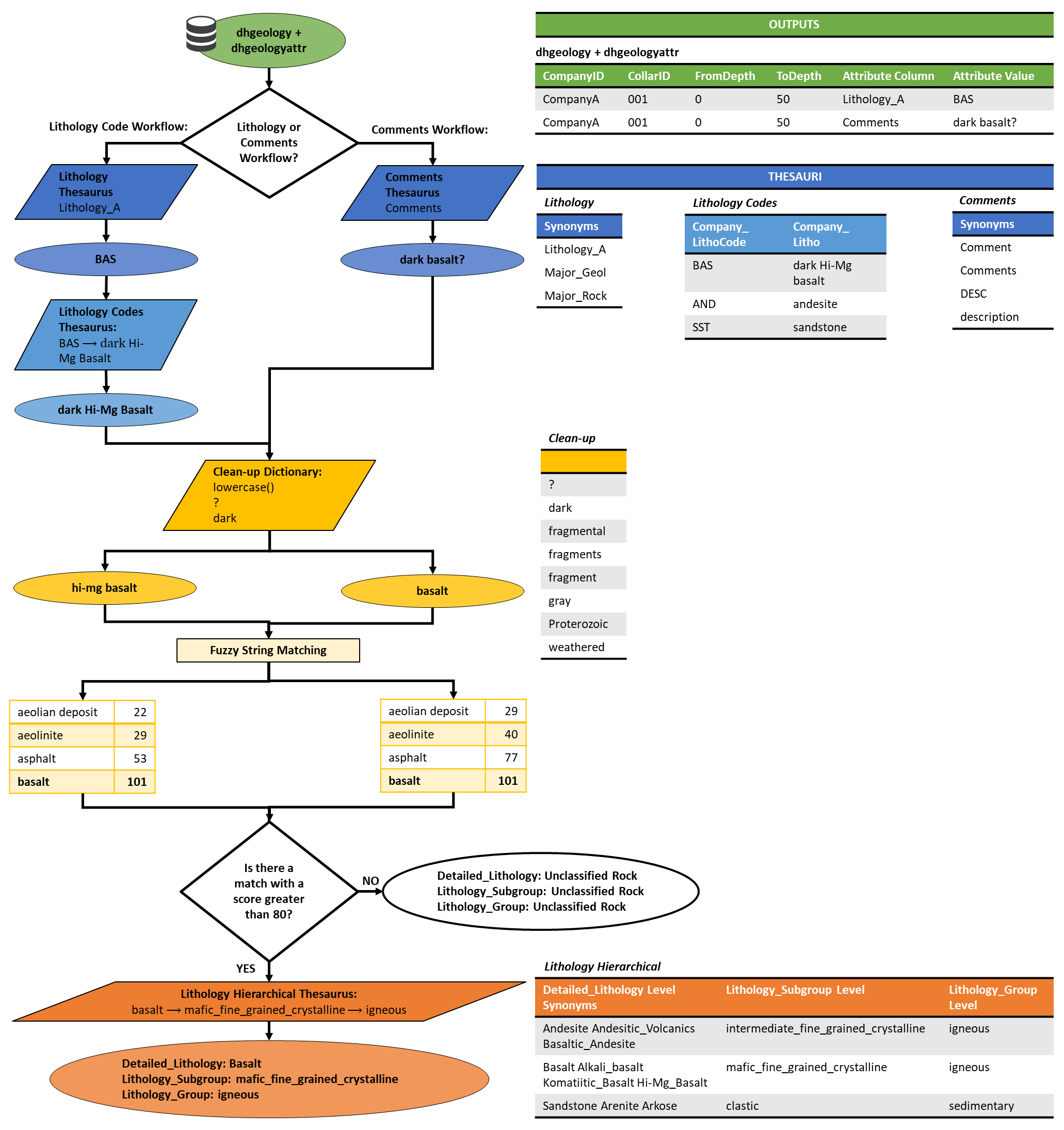
Figure 2Lithology extraction is done through the Lithology Code workflow
and Comments workflow. The values are fetched from the dhgeology and dhgeologyattr table (green)
using either the Drill Hole Lithology Thesaurus (blue) and Drill Hole
Lithology Codes Thesaurus (light blue) or the Drill Hole Comments Thesaurus
(blue). The string fetched is then cleaned prior to the fuzzy string
matching using the Clean-up Dictionary (dark yellow). The result is then
matched against the Detailed_Lithology level of the
Lithological Hierarchical Thesaurus. If there is a match with a score
greater or equal to 80, the match is taken and matched with the rest of the
columns in the Lithology Hierarchical Thesaurus. If not, it is labelled as
unclassified rock.
Once the Company_Litho (decoded lithology from
Company_LithoCode or from the Comments (free-text
descriptions) has been extracted from the database, the lithology strings
are pre-processed such that
- a.
the strings are converted to lowercase form;
- b.
the strings inside parenthesis, brackets and braces are removed, as these are found to reduce the accuracy of the matching;
- c.
the strings preceded by key phrases such as “with”, “possibly” and “similar to” are removed;
- d.
if any of the words listed in the Clean-up Dictionary are present in the string, these words are removed;
- e.
lemmatization, the removal of the inflections at the end of the words in order to obtain the “lemma” or root of the words, is applied to all nouns (Müller et al., 2015);
- f.
all words with non-alphabetic characters and tokens with less than three characters are removed; this includes two-letter words such as “to”, “in” and “at”;
- g.
stopwords, a set of words frequently used in language which are irrelevant for text mining purposes (Wilbur and Sirotkin, 1992), are removed. Examples of stopwords are as follows: “as”, “the”, “is”, “at”, “which” and “on”.
This is followed by fuzzy string matching, a technique that finds the string that matches a pattern approximately. Fuzzy string matching is typically divided into two sub-problems: (1) finding approximate substring matches inside a given string and (2) finding dictionary strings that match the pattern approximately. Fuzzy string matching uses the Levenshtein distance to calculate the differences between sequences and patterns (Okuda et al., 1976; Cohen, 2011). The Levenshtein distance measures the minimum number of single-character edits (insertion, deletion, substitution) necessary to convert a given string into an exact match with the dictionary string (Levenshtein, 1965).
We utilize fuzzywuzzy (https://github.com/seatgeek/fuzzywuzzy, last access: 30 September 2021) for this.
fuzzywuzzy provides two methods to calculate a similarity score between two strings:
ratio() or partial_ratio(). It also provides two functions to pre-process the strings:
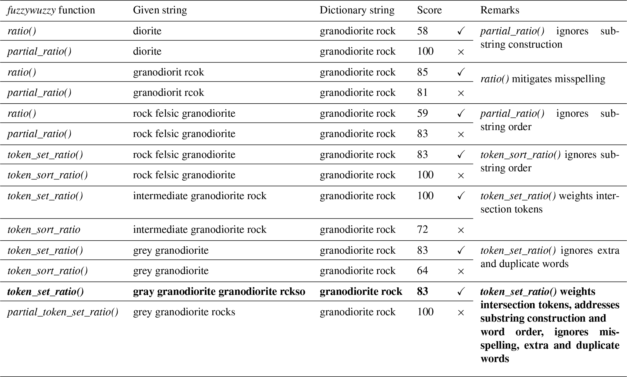
token_sort() and token_set(). In this work, we used the token_set_ratio() scorer to do fuzzy string matching to
classify the Company_Litho or Comments entries as one of
the Lithology Hierarchical Thesaurus entries (Table 1). token_set() pre-processes the strings by (1) splitting the string on white spaces
(tokenization), (2) turning to lowercase, and (3) removing punctuation,
non-alpha, non-numeric characters and unicode symbols. It tokenizes both
strings (given string and dictionary string), splits the tokens into intersection and remainder, and then sorts and compares the strings. The sorted
intersection component refers to the similar tokens between the two strings.
Since the sorted intersection component (similar tokens between two strings)
of token_set(), will result in an exact match, the score will tend to increase
when (1) the sorted intersection makes up a larger percentage of the full
string and (2) the remainder components are more similar. The ratio() method then
computes the standard Levenshtein distance between two strings.
token_set_ratio() is found to be effective in addressing harmless misspelling and duplicated
words but sensitive enough to calculate lower scores for longer strings
(3–10 word labels), inconsistent word order, and missing or extra words.
partial_ratio(), which takes the best partial of two strings or the best matching on the
shorter substring, is not preferred as it does not address the difference and
order in substring construction. token_sort() is not preferred as it alphabetically sorts
the tokens that ignore word order and does not weight intersection tokens
which do not address the behaviour of the strings in the logs.
Table 1Examples of fuzzy string matching output using different combinations of the fuzzywuzzy functions. The ticks and crosses beside the score indicate the preferred (ticks) result between the methods clustered together. The item in bold is the preferred method for this work.
dh2loop calculates the token_set_ratio() between the Company_Litho or Comments
(given string) and the entries in the Lithology Hierarchical Thesaurus
(dictionary string). The tendency is to enumerate the descriptors before the
rock name. For example, if the lithology in the logged interval is
“basalt”, the free-text description could be something like “Dark grey to
dark reddish brown, with olivine phenocrysts, largely altered andesitic
basalt”. After processing the string, it will be left with “andesitic
basalt”. To avoid misclassifying the rock as “andesite”, a bonus score
is also added to add weight to the last word (in this case, “basalt”).
Furthermore, the reader may worry that “basaltic andesite” will be
simplified and classified as “andesite”. Since “basaltic andesite” is
an established volcanic rock name, it will remain “basaltic andesite”.
For the pair between Company_Litho or Comments and the
entries in the Lithology Hierarchical Thesaurus with the highest score, the
first synonym is stored as Detailed_Lithology. If the score
is less than 80, it is classified as “unclassified rock”. The cut-off
value is user-defined and can be chosen based on the performance of the
matching on the subset of the desired region. If the performance is
significantly lower, this indicates that the thesauri used in dh2loop may not be
suitable to your area. The user may opt to update these thesauri to suit
their needs. Once matched on Detailed_Lithology, the
corresponding Lithology_Subgroup and Lithology_Group classifications are also fetched.
2.5 Fuzzy string matching assessment
The objective is to compare the Detailed_Lithology
classification results obtained from two independent workflows: the (1)
Lithology Code workflow and (2) Comments workflow.
Using the Company_LithoCode, Company_Litho,
Lithology Code workflow: Detailed_Lithology and
Comments workflow: Detailed_Lithology from the
dataset for the fuzzy string matching assessment, we can assess whether matches
using the Comments workflow alone can sufficiently decode
lithology.
To be able to assess the matching we take a look at the type of matches
between Lithology Code workflow: Detailed_Lithology
and Comments workflow: Detailed_Lithology. First, we
define a match as retrieving an answer from the fuzzy string
matching with a score greater than 80. It is important to note here that it
only suggests that it succeeded in finding an answer above the score threshold
but it does not necessarily mean that it is the correct answer. To further describe
the quality of a match, we modified the following terms from the Simple Knowledge Organization System (Miles and
Bechhofer, 2009) for this purpose:
- a.
“Exact match” suggests that both Lithology Code workflow and Comments workflow resulted in the same classification at all three levels. The match at the
Detailed_Lithologylevel has an exact match, thus resulting in an exact match on the other two levels. - b.
“Close match” suggests that the results at the
Detailed_Lithologylevel are related rocks and belong to the sameLithology_Subgroup. This is usually caused by differing use of lithological nomenclature. - c.
“Related match” suggests that the results at the
Detailed_Lithologylevel are related rocks and belong to the sameLithology_Group. - d.
“Broad match” refers to the
Detailed_Lithologyfrom Lithology Code workflow matches aLithology_Subgroupin the Comments workflow. - e.
“Narrow match” is the logical equivalent of a broad match. In this case, the Comments workflow resulted in a
Detailed_Lithologylevel, while the Lithology Code workflow resulted in aLithology_Subgrouplevel. - f.
“Broader match” is similar to a broad match except that the
Detailed_Lithologyfrom Lithology Code workflow matches aLithology_Groupinstead of aLithology_Subgroupin the Comments workflow. - g.
“Narrower match” is the logical equivalent of broader match. The Comments workflow results in a
Detailed_Lithologywhile the Lithology Code workflow results in aLithology_Grouplevel. - h.
“Failed match” suggests all levels of both workflows do not match. This is usually attributed to contrasting information from both fields or the algorithm fails. This category is an addition to the Simple Knowledge Organization System (SKOS) reference.
For better understanding of these relationships, examples are shown in Table 2 and Fig. 3.
Table 2Fuzzy string matching terminology used to describe the quality of
matches based on the Simple Knowledge Organization System (SKOS) (Miles
and Bechhofer, 2009). The values being compared are the
Detailed_Lithology level for both the Lithology Code workflow and Comments workflow. The level at which the records are considered to match
are in bold.
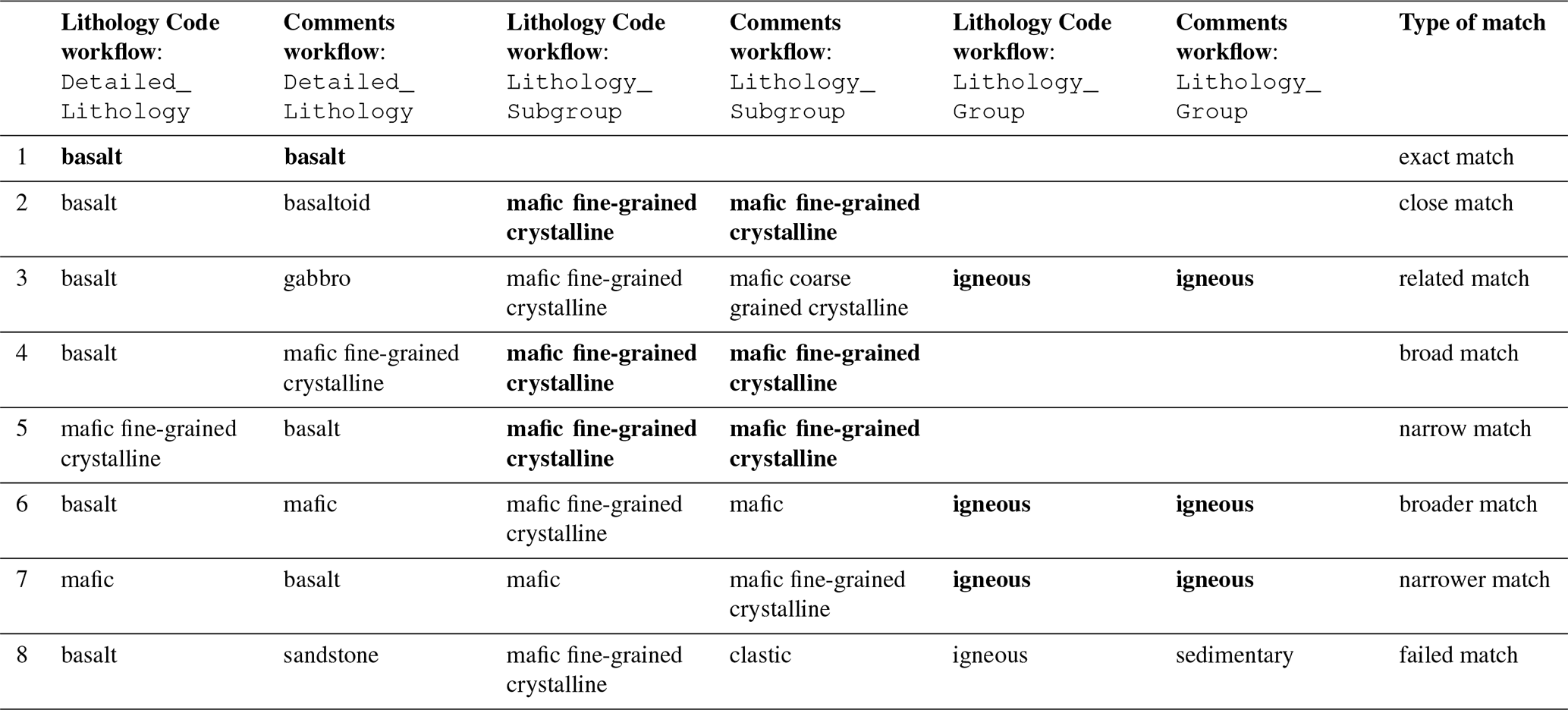

Figure 3SKOS graph showing the semantic, associative and hierarchical relationship in the Lithology Hierarchical Thesaurus. In this example, the terms “basalt” and “alkali basalt” are judged to be sufficiently the same to assert an exact match relationship (in green). “Basic volcanic rock” however is considered a close match (in cyan) and “gabbro” a related match (in blue). “Mafic fine-grained crystalline” and “mafic coarse-grained crystalline” are broader concepts and are thus considered a broad match (in orange) with “basalt” and “gabbro”, respectively. Broader match (in brown) is similar to broad matches but is used to refer a wider semantic difference between the two concepts. Narrow matches (in light purple) and narrower matches (in dark purple) are the logical equivalent of broad match and broader match. Failed matches is used to describe unrelated matches.
The matching results can be visualized as confusion matrices, which are typically used in machine learning to compare the performance of an algorithm versus a known result. In this case, we are comparing the performance of the string matching using the Comments workflow against the results from the Lithology Code workflow. Each row of the matrix represents the matched lithology from the Comments workflow, while each column represents the matched lithology from the Lithology Code workflow. The diagonal elements represent the count for which the Comments workflow class is equal to the Lithology Code workflow. The off-diagonal elements are those that are misclassified by the Comments workflow. The higher the diagonal values of the confusion matrix the better, indicating many correct matches. The confusion matrices show normalization by class support size. This kind of normalization addresses the class imbalance and allows better visual interpretation of which class is being misclassified. The colour of the cell represents the normalized count of the records to address the uneven distribution of records across different classes. Relying on one metric to assess the matching can be misleading, therefore, we would like to use four metrics: accuracy, precision, recall and F1 score. It is worth mentioning that a small support influences the precision and recall. However, this is the nature of using real-world geological logs as more detail is given to particular lithologies or areas, depending on the interest of the study.
3.1 Study area
In this paper, we demonstrate the application of dh2loop to data from the Yalgoo–Singleton greenstone belt (YSGB) (Fig. 4), a geologically complex, largely heterogeneous and highly mineralized arcuate granite–greenstone terrane, in the western Youanmi Terrane, Yilgarn Craton, in Western Australia (Anand and Butt, 2010). The YSGB has good range of different lithologies in the area. Igneous rocks occur as extensive granitoid intrusions emplaced between 2700 and 2630 Ma (Myers, 1993), as well as ultramafic to mafic volcanic rocks formed as extensive submarine lavas and local eruptive centres of felsic and mafic volcanic rocks. Some layered gabbroic sills intruding the greenstone are also observed. Sedimentary rocks formed in broad basins during tectonic and volcanic quiescence consist of mostly banded iron formation (BIF) and felsic volcaniclastic rocks. The greenstone belt is metamorphosed to greenschist facies (Barley et al., 2008). The area is also covered by deeply weathered regolith which conceals mineral deposits hosted by the underlying bedrock. Regolith contains signatures of mineralization that are distal signatures of possible economically significant deposits (Cockbain, 2002). Furthermore, the YSGB is a major target for exploration as it has considerable resources of gold, nickel and bauxite as well as lesser amounts of a wide range of other commodities (Cockbain, 2002). It hosts multiple mineral deposits ranging from volcanogenic massive sulfide (Golden Grove, Gossan Hill) to orogenic gold (Mt. Magnet) to banded iron formations (Mount Gibson, Karara, Extension Hill). The geological and structural complexity, including its relevance to mineral exploration makes the YSGB a reasonable and sensible area to test the dh2loop thesauri, matching and upscaling.
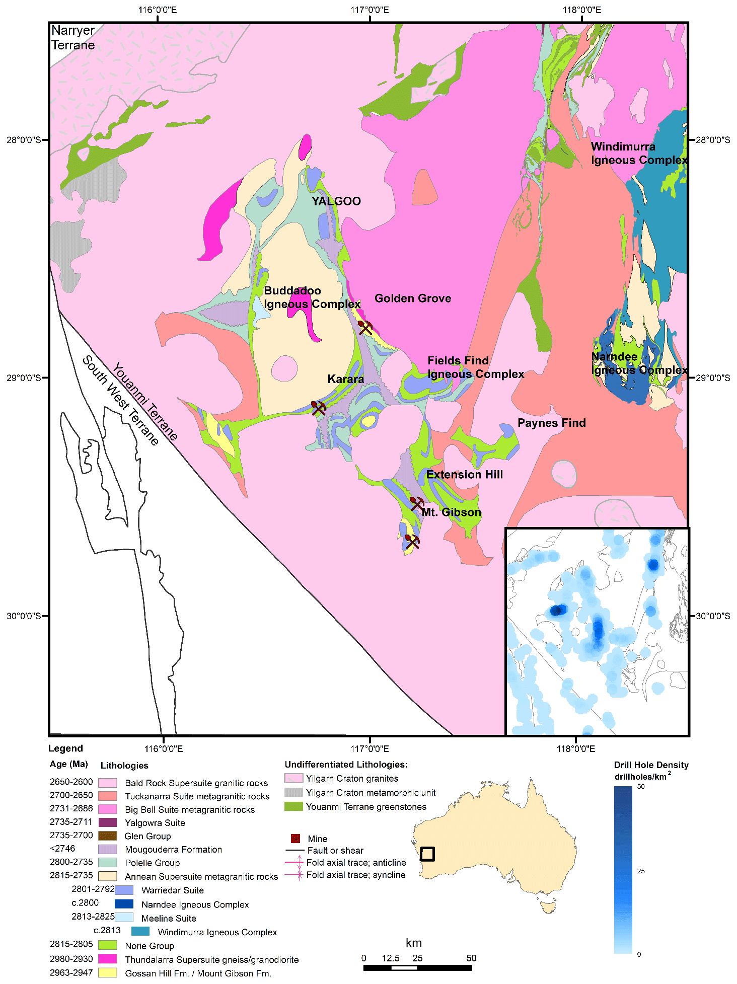
Figure 4The map shows the Yalgoo–Singleton greenstone belt highlighting the different mines and prospects in the area. The inset map shows the heterogeneous distribution and drill hole density from the legacy data available from the WAMEX database.
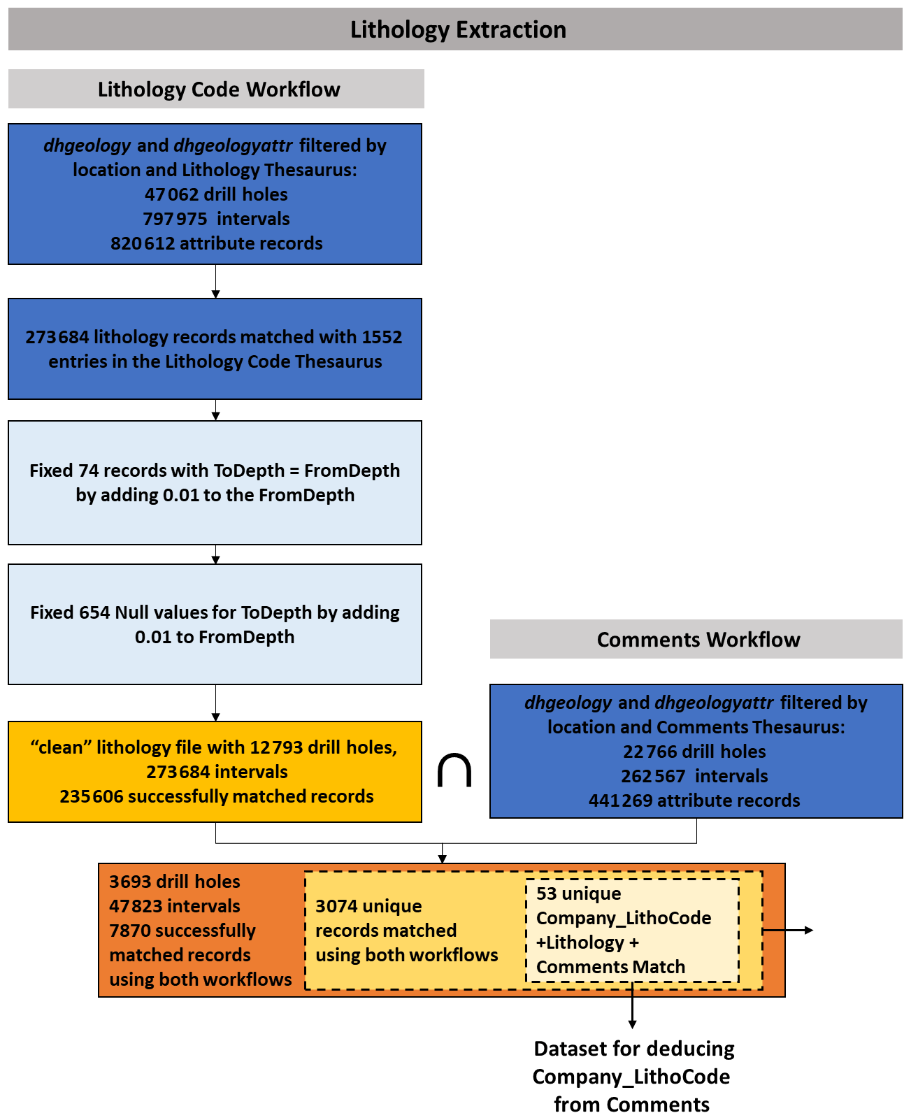
Figure 5Extraction of lithology data for the YSGB. For the Lithology Code workflow, the extraction starts with filtering the dhgeology and dhgeologyattr table by the
location extents and the Drill Hole Lithology Thesaurus. These records are
matched with the entries from the Lithology Code Thesaurus. The Lithology Code workflow resulted in 235 606 records successfully matched in the fuzzy
string matching. The Comments workflow extracts the records from the
dhgeology and dhgeologyattr table as well, but this time using the Drill Hole Comments Thesaurus.
In total, 47 823 records are present in both workflows, 7870 records of which are
successfully matched. The 3074 unique entries from this are used as the
dataset for the fuzzy string matching assessment.
3.2 Lithology extraction: Lithology Code workflow and Comment workflow
Lithology extraction is divided into two workflows. For the
Lithology Code workflow, the extraction starts with filtering the
dhgeology and dhgeologyattr table by the location extents and the Drill Hole Lithology Thesaurus.
The dhgeology table contained 47 062 drill holes across 115 companies with 797 975
lithology depth intervals with a corresponding 820 612 entries of lithology
information in dhgeologyattr (Fig. 5). These records are matched with the entries from the Drill
Hole Lithology Codes Thesaurus resulting in 273 684 matched records. The
FromDepth and ToDepth for these records are then validated. In total, 74 records had
equal FromDepth and ToDepth values. In total, 654 had values for FromDepth but null
values for ToDepth. For both cases, ToDepth is calculated as
FromDepth + 0.01. The cut-off value of 80 is used for the string matching
based on the performance of the matching in a subset of 1548 unique
lithology codes from the Golden Grove area (Fig. 6). The Lithology Code workflow resulted in 273 684 intervals across 12 793 drill holes
wherein 235 606 records are successfully matched in the fuzzy string
matching. The remaining 546 819 entries did not obtain a match with a score
greater than 80. An example of unmatched entries is provided in Table 2.
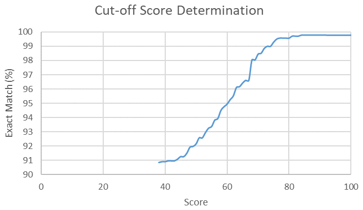
Figure 6The user-defined cut-off score of 80 is chosen based on the results of the testing of different cut-offs on a smaller dataset within the YSGB area. As seen in this figure, the number of exact matches plateau at a score of 80.
The Comments workflow extracts the records from the dhgeology and
dhgeologyattr table as well, but this time using the Drill Hole Comments Thesaurus. For
YSGB, the database has 262 567 records across 22 766 drill holes with free-text descriptions. In total, 47 823 records are present in both workflow. Since the
free-text descriptions are extracted here to compare their results from
fuzzy string matching, only 7870 records that also matched (both have a
score greater than 80) in the Lithology Code workflow are retained.
3.3 Fuzzy string matching results
We present results from the data extraction using both workflows:
Lithology Code and Comments. The dataset for the fuzzy
string matching assessment consists only of the unique records matched on
both Lithology Code workflow and Comments workflow (3074
records). It is visually checked from the records that the Lithology Code workflow: Detailed_Lithology results are sound
classifications of the Company_Litho. This is done to make
sure that these results could be regarded as the true value in the
fuzzy string matching assessment. The overlaps between these two workflows
suggest that the user may need to make choices to identify which is better
suited for matching in their area of interest. To better understand the
difference between these results, we looked at the matching overlaps between
the two workflows (3074 entries). These matching overlaps are used to
compare and describe the fuzzy string matching using the decoding the
Company_LithoCode and using Comments.
We also take a look at the unique combinations of Company_LithoCode, Company_Litho, Lithology Code workflow:
Detailed_Lithology and Comments workflow:
Detailed_Lithology (53 unique records from the 3074
records). In total, 34 out of the 53 unique entries (64 %) result in matches between
the Lithology Code workflow: Detailed_Lithology and Comments workflow: Detailed_Lithology. Of these, 26 are exact matches,
19 unique entries are close matches and 26 % percent are failed matches.
The failed matches are due to unrelated descriptions in the Comments field
which is used to obtain the results in Comments workflow:
Detailed_Lithology. An example of this is the interval logged as “ironstone” (Company_Litho), but Comments contains
“mafic schist”. Another less common reason is that Company_LithoCode is repeated in the Comments. An example of this is would be an
interval logged as “colluvium” (Company_Litho) and the Comments as “COL”. The Comments workflow will result in “coal” instead.
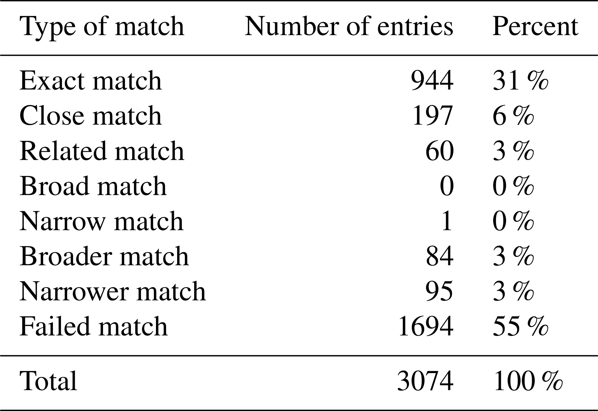
-
Exact matches: of the total matched entries, 944 are exact matches (31 %) (Table 2). The exact matches are ideal outcomes as both workflows resulted in exactly the same answers.
-
Close matches: the close matches are common for coarse-grained igneous rocks, clastic sedimentary rocks, surficial residual rocks and filling structures. The coarse-grained igneous rocks such as gabbro, gabbroids and dolerites are used interchangeably in both fields.
Commentscan contain terms such as “gabbroic”, “granophyric gabbro to dolerite” or “intrusive granitoid to gabbro” resulting in close matches. Similar cases are observed between granodiorite and granite and between peridotite and coarse-grained ultramafic rocks. For clastic sedimentary rocks, the close matches are a result of gradation of grain size in theComments. For example, an interval logged as mudstone (Company_Litho) is then described inCommentsas “mudstone to sandstone” or “intercalated with siltstone”.Commentsentries like this will result in “sandstone” and “siltstone”, respectively. Both are clastic sedimentary rocks but not an exact match to mudstone. Metasediments and quartz veins occur together, and what is described last dictates theDetailed_Lithologyclassification. Surficial rocks such as soil, duricrust, colluvium, laterite, calcrete, ferricrete and cover are used loosely or occur together, resulting in multiple combinations of these close matches. -
Related matches: a total of 60 entries (3 %) resulted in related matches. For igneous rocks, this result is observed when
Commentsuse rock type descriptors such as “komatiitic”, “basaltic” and “doleritic”. An example would be an interval logged as dolerite and then described inCommentsas “doleritic basalt”. This would result in dolerite in the Lithology Code workflow and “basalt” in the Comments workflow. Both lithologies are igneous but have a different composition and textural implications. For sedimentary rocks, Lithology Code workflow results in sedimentary rocks classified based on grain size as they have been logged (“gravel”, “mud”). TheCommentscontains compositional descriptions such as “with silcrete” or “minor chert”. In this case, the Comments workflow will result in “silcrete” and “chert”. Both workflows will result in sedimentary rocks, but the Lithology Code workflow will result in “clastic” rocks while the Comments workflow will classify these to “siliceous” at theLithology_Subgrouplevel. The related matches for structures occur across coincident lithologies such as “mylonite”, “vein”, “fault” and “breccia”, which could either be “fillings” or “fault_rock” in theLithology_Subgroup. -
Broad and narrow matches: no broad matches are noted and only one narrow match is obtained (Table 3). The interval is logged as “ironstone” with “BIF” in
Comments, “ironstone” being a more general description for “banded iron formation”. -
Broader and narrower matches: more common cases are broader and narrower matches, indicating that there is a bigger relationship gap between the data in
Company_LithoandComments. Broad matches are a result of low-detail free-text descriptions inComments. For example, an interval logged as “gabbro” is described as “medium-grained mafic”, “massive mafic” or “rich mafic”. The inverse is noted for narrower matches; the interval is logged as “sediment”, but inCommentsthe interval is described as “siliceous sediments”. -
Failed matches: a total of 1694 entries resulted in failed matches (55 %). Failed matches occur when
Company_LithoandCommentscontain different information. This could be because theCompany_Lithocontains the main lithology whileCommentscontains all other lithologies intercalated in the interval. Another reason is thatCompany_Lithois re-logged based on adjacent intervals without amendingComments. “Mudstone” had failed matches with a wide range of lithologies, such as “amphibolite”, “dolerite”, “saprolite”, “duricrust”, “laterite”, “banded iron formation”, “chert”, “phyllite”, “schist” and “vein”. The same is observed for igneous rocks such as “coarse-grained ultramafic rock”. For “chert”, the failed matches are within a range of sedimentary rocks: “alluvium” and “mud”, “amphibolite” and “massive sulfide”, “carbonate”, “vein” and “pegmatite”.
Table 3Distribution of matches across the fuzzy string matching dataset. A total of 45 % of the unique records are matched reasonably, 31 % of which are exact matches, 6 % close matches, 3 % related matches, 3 % Broader matches and 3 % narrower matches.
The matching results are visualized as confusion matrices, comparing the performance of the string matching using the Comments workflow against the results from the Lithology Code workflow. From the 3074 unique records, we use a total of 1200 samples for the confusion matrices. The reason for this difference is the limitation of building a confusion matrix wherein both workflows look at the same classes and ensuring that both workflows produce a match.
3.3.1 Structure and texture
While geological structures are not lithologies, they are sometimes described in lithological logs (Fig. 7). Structures common in the YSGB area are faults and veins. Figure 7 shows the confusion matrix for the structures and textures. The vertical axis represents the matches from the Lithology Code workflow while the horizontal axis for the results from the Comments workflow. We consider a dataset of 52 unique records where we are trying to assess whether the Comments workflow results in the same classification as the Lithology Code workflow. Figure 7 shows that there are 6 records classified as “fault” and 46 records as “vein”. When looking at the classification of “faults” we can say that there are two records that are true positives. In total, 46 records are true negative pairs, as in this 2 × 2 matrix, if it is not a “fault”, it is a “vein”. True negatives together with true positives are the exact matches and suggests that the Comments workflow identified it correctly. To have a better look at the parts that are not classified correctly we look at the false positives and false negatives. False positives represent the number of records classified as “fault” but based on the Lithology Code workflow are not. In this case, there are no false positive values. False negatives represent number of records classified as “vein” but are actually “faults” based on the Lithology Code workflow.
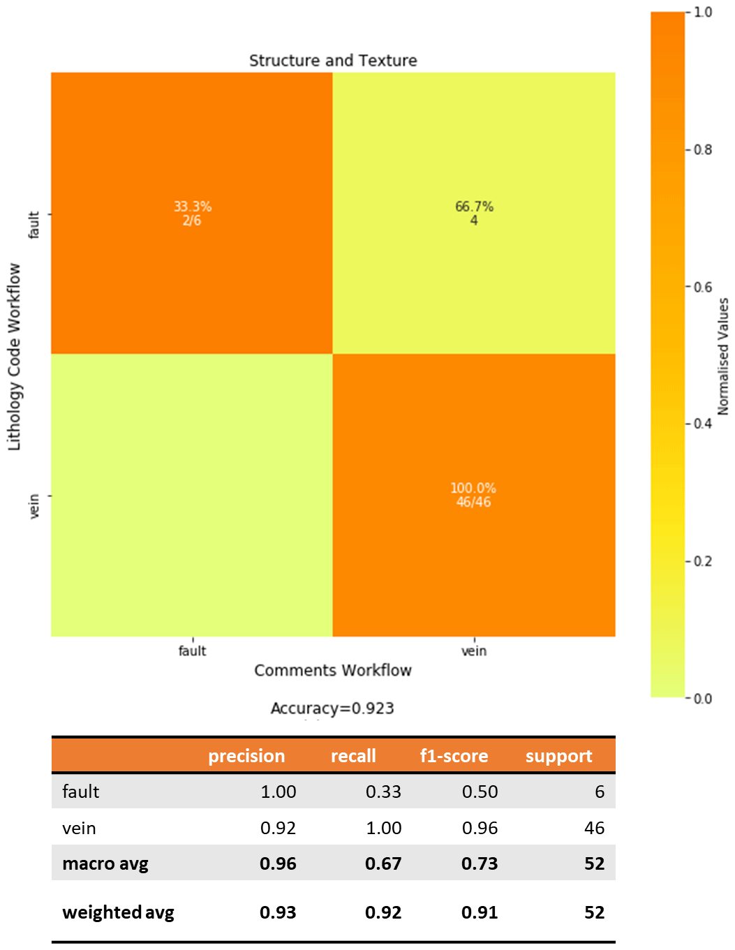
Figure 7Confusion matrix for structure and texture comparing the fuzzy
string matching results from the Lithology Code workflow (vertical axis) and
Comments workflow (horizontal axis). The heatmap shows the values normalized
to the support size to address the imbalance between classes. The values
shown in the cells indicate the number of samples classified for the class.
Empty cells indicate zero samples. The structures and texture
Lithology_Group had an accuracy of 92.3 % across 52
samples: 46 for veins and 6 for faults.
A total of 48 exact matches are noted, 46 records of which are “veins” and
2 records are “faults”. This can be surmised by looking into the diagonal
cells. The rest of the “veins” (4 records) are related matches as
“faults”. They are considered related matches as faults and veins tend to
coexist in nature. In addition, faults often occur as fault zones, with
infill clay or silica vein sulfides which are described in Comments that
then obscures the classification. These structure-related lithological
descriptions can be used as proxies in further geological studies.
3.3.2 Igneous rocks
The confusion matrix for igneous rocks considers a dataset of 218 unique records (Fig. 8). Dealing with a larger matrix is not as straight-forward as the previous matrix. When looking at the classification of a single lithology, the true positives are where both axes refer to the same class. For example, for “basalt” there are 15 records of true positives which correspond to the exact matches. The false positives are the sum of all the other entries along the corresponding vertical axis, and the false negatives are the sum of all the entries along the corresponding horizontal axis. The sum of all the other cells represent the true negatives. For “basalt”, there are 15 true positives, 13 false positives, 15 false negatives and 175 true negatives. This results in 54 % classification precision for “basalt”.
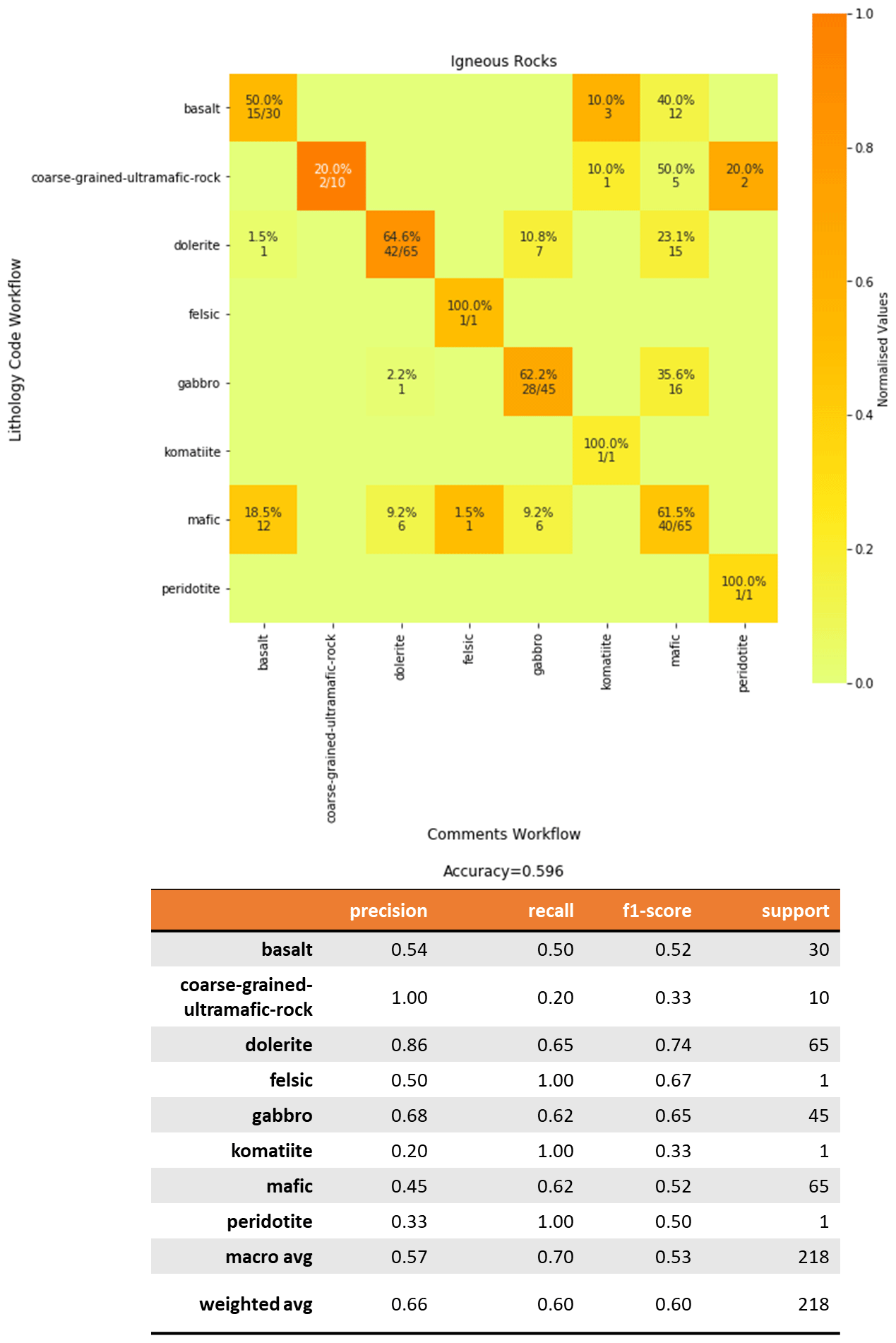
Figure 8Confusion matrix for igneous rocks comparing the fuzzy string matching results from the Lithology_Code workflow (vertical axis) and Comments workflow (horizontal axis). The heatmap shows the values normalized to the support size to address the imbalance between classes. The values shown in the cells indicate the number of samples classified for the class. Empty cells indicate zero samples.
This statistic is helpful in quantifying the performance of the
classification. However, what it does not capture is the semantic and
hierarchical relationship of the false negative pairs. As shown in Figs. 8,
3 records are classified as “komatiite” and 12 records are classified as
“mafic”. The “komatiite” matches are a result of when Comments describe
the basalts as “komatiitic basalts”. This can be regarded as a related
match. The 12 records which are classified as “mafic” are considered a “broader match”. For the false positive values, the “mafic” records are
narrower matches while the “dolerite” is a related match. These
quantitative assessments of the matches show us that although the matching is
not perfect, the context of the misclassification is not severe.
“Dolerite” is the most common igneous rock matched. This could be
attributed to the sampling bias towards dolerite as it is often targeted by
drilling as it is used as targeting criteria for gold mineralization
(Groves et al., 2000). Given that dolerites can be described by their
mafic component or be confused as gabbro when weathered, the descriptions
contain the strings “mafic” and “gabbro” which explain close and broader
matches. Gabbros are also common in the YSGB. Some of the “gabbros” are
classified as “mafic” in the Comments Detailed_Lithology.
This is another example of a broader match. However, it is important to note
that although it is not an exact match, a broader match can be useful in
geological studies relating to rock composition as gabbros are members of
mafic rocks. In total, 40 % of the igneous rock that are mismatched at the
Detailed_Lithology level are broader matches (matches
correctly at Lithology_Group).
3.3.3 Sedimentary rocks
The largest Lithology_Group of the lithological entries
relates to sedimentary rocks (800 entries) (Fig. 9). In total, 457 of the 800 entries
are true positive classification of mudstones. Mudstones are common as shale
beds. Mudstones resulted in related matches with “chert” and
“ironstone”. The misclassification occurs when the logs describe intervals
wherein the mudstone occurs together and is intercalated with these
lithologies. A few mudstones (17) are matched as sandstone due to textural
and grain size descriptors (close match). In total, 48 % of the cherts resulted
in exact matches. In total, 39 records of cherts resulted in failed matches as their
Detailed_Lithology level matched with “banded iron
formation”; it occurs when intercalated, such as “cherts with
BIF”, or includes string descriptors, such as “BIF-fy”.
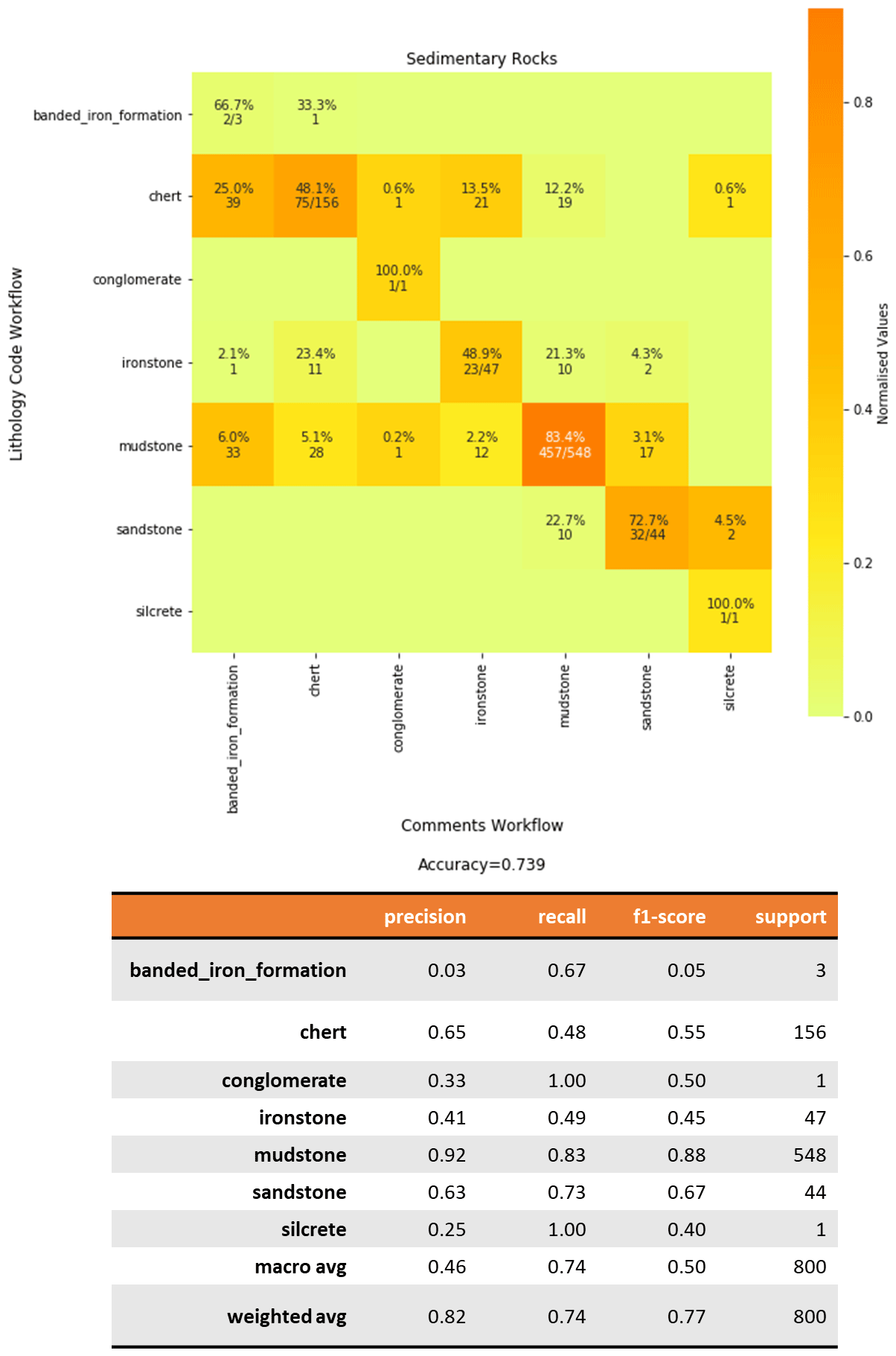
Figure 9Confusion matrix for sedimentary rocks comparing the fuzzy string matching results from the Lithology Code workflow (vertical axis) and Comments workflow (horizontal axis). The heatmap shows the values normalized to the support size to address the imbalance between classes. The values shown in the cells indicate the number of samples classified for the class. Empty cells indicate zero samples.
3.3.4 Metamorphic rocks
Out of a total of 61 metamorphic rock entries, 60 are matched correctly (Fig. 10). Most of these are “schists” as the YSGB area is rich in
talc–carbonate schists. The Company_Litho entry “amphibolite
mica schist”, which is matched as “amphibolite”, matches as “schist” in
the Comments workflow. This is considered a related match.
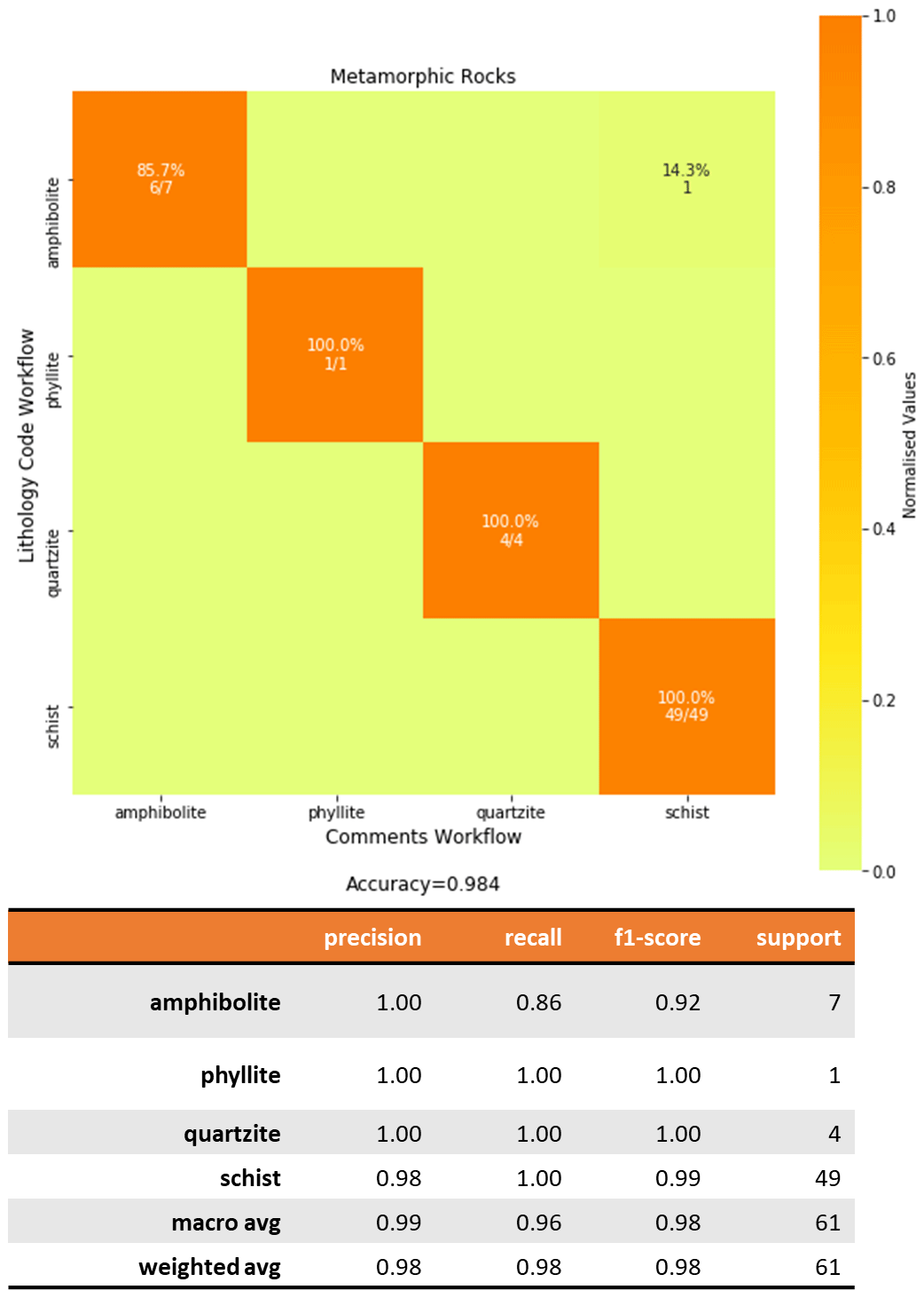
Figure 10Confusion matrix for metamorphic rocks comparing the fuzzy string matching results from the Lithology Code workflow (vertical axis) and Comments workflow (horizontal axis). The heatmap shows the values normalized to the support size to address the imbalance between classes. The values shown in the cells indicate the number of samples classified for the class. Empty cells indicate zero samples.
3.3.5 Surficial rocks
Fuzzy string matching accuracy of surficial rocks scored 45 % on a total
of 69 entries (Fig. 11). Saprolites are matched as saprolite (exact match),
rock (failed match) and saprock (close match). In instances where saprock is
inputted as “sap rock”, it results in a failed match as “rock”. “Soil”
is commonly used in logs to refer to the first intercept of highly
weathered, clay-rich and unidentifiable intercept. “Soil” is classified
with the highest variability of terms: “soil” (exact match), “rock”
(failed match), “duricrust” (close match), “colluvium” (related match)
and “calcrete” (close match). “Laterite” is matched to “colluvium”
(related match), “duricrust” (close match) and “lag” (close match).
“Lag” generally matches with “colluvium” (related match). However, when
described in Comments, it can be associated with its protolith which results in a failed match as “rock”.
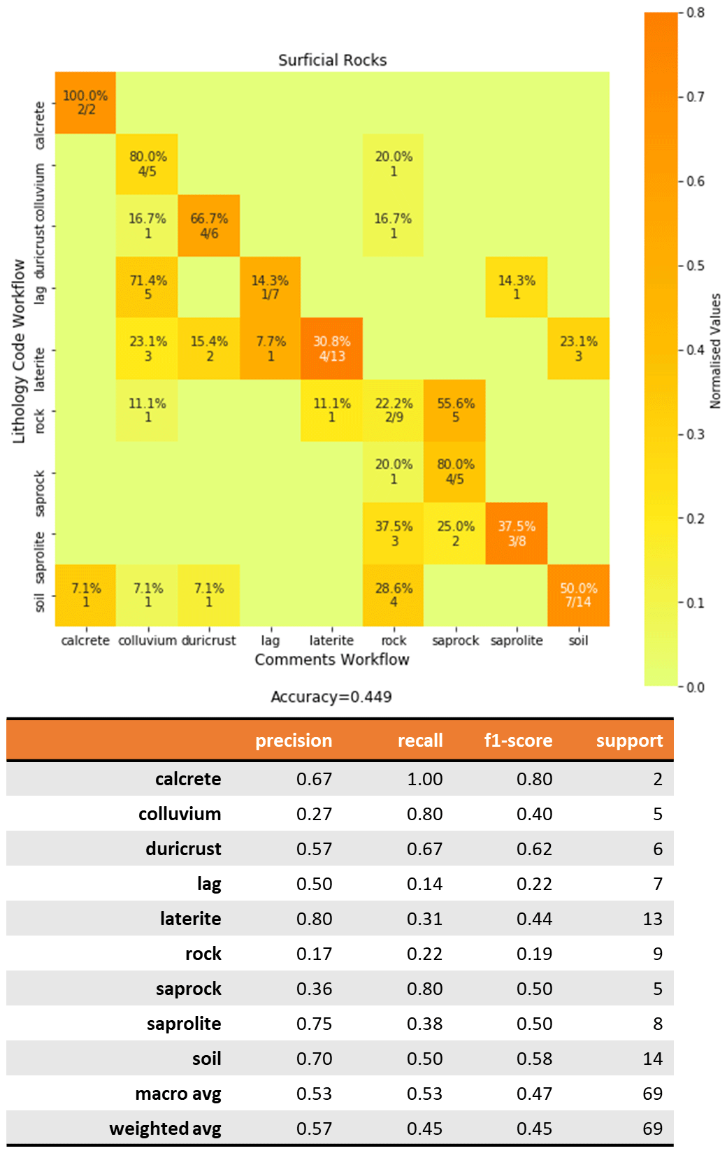
Figure 11Confusion matrix for surficial rocks comparing the fuzzy string matching results from the Lithology Code workflow (vertical axis) and Comments workflow (horizontal axis). The heatmap shows the values normalized to the support size to address the imbalance between classes. The values shown in the cells indicate the number of samples classified for the class. Empty cells indicate zero samples.
4.1 dh2loop functions and notebooks
The dh2loop library supports a workflow that extracts, processes and classifies lithological logs (Appendix A4). This library is built to extract drill hole logs from the WAMEX database. The assumptions made in the entire workflow attempt to replicate the thought process of a geologist performing the data extraction, data quality checks and lithological log classification manually. However, it can be adapted for other geological relational databases or from other table formats. An example using comma-separated values tables (CSVs) is shown in the notebook Exporting and Text Parsing of Drillhole Data Demo.
In addition to the data extraction, downhole de-surveying and lithological matching functions discussed, dh2loop also provides functionalities and a notebook demonstrating harmonization of drill hole data. This is useful for combining and correlating drill hole exports of different properties such as lithology, assays and alteration. It is also possible to export this information in Visualization Toolkit format (.VTK). It also provides a notebook that demonstrates the application of lasio and striplog on dh2loop interval table exports. WAMEX reports can also be interactively downloaded through a notebook provided in the package.
4.2 Thesauri
dh2loop provides the user with nine thesauri that deal with the extraction of collar, survey and lithology interval tables. For the extraction of other properties, such as downhole alteration, geochemistry, mineralogy and structures, at least one thesaurus is needed for each attribute we would like to export. These thesauri are built manually by inspecting all the terminologies available in the database. Although creating them can be tedious, updating an existing thesaurus is as simple as adding and/or removing a word for the list. There are many other properties available in the database that could be exploited using the existing methodology; thus there is an incentive in finding a way to improve the methodology of building these thesauri. Analysis on the syntax of the existing thesauri may help in automating the creation of other thesauri.
The Hierarchical Lithology Thesaurus puts equal weight on each of the entries in the thesaurus. By knowing the geology in a user's area, the matching can be improved by adding more weight to prevalent lithologies through adding a bonus score.
4.3 Data extraction
dh2loop supports the data extraction of collar, survey and lithology interval tables. The main consideration in the data extraction is that the data retrieved are complete, relevant and useful. We would rather throw erroneous or questionable data out and have the rest with a high level of confidence than the other way around. The lithology extraction using the Lithology Code workflow shows that the bottle neck to its extraction rate is the extensiveness of the Drill Hole Lithology Codes Thesaurus. Since the thesaurus did not have information for all companies in the area, only 34 % of the available information is retrieved. The extraction results for the Comments workflow cannot be compared with the Lithology Code workflow as only the intersection of both workflows is considered in this study.
4.4 Assessment of string matching results
The number of successful matches are dependent on the selected cut-off score. The selection of a cut-off score is a balance between the number of matched records and the exact match percentage. In this case study, we selected a cut-off score of 80 since this is where the number of exact matches plateaus (Fig. 6). A lower cut-off score could be used, depending on the familiarity with the data and/or the purpose of the drill hole processing. For our case, we wanted to be as conservative as possible without being too stringent (cut-off score 100).
The string matching results highlight that geological drill core logging is
prone to human error and bias and results in incorrect logs. Sometimes even
if the data are available and correct, they are not in a format that can be
directly extracted. For example, Comments are filled with a string
description such as “same as above” and “-do-“. Currently, for this
case, dh2loop returns without a match, as replacing “same as above” requires
building a dictionary for all possible permutations to refer to this. This
is not included in the scope of this work. In the future, we could be able
to search through the previous entries to retrieve the correct lithology.
Furthermore, the code does not handle and check for inconsistencies in the
logs. It only addresses the inconsistencies in nomenclature and not the
logging itself. The string matching misclassification results illustrate
the importance in the consistency and level of detail being put into
logging and identify differences in convention or uncoordinated logging
among geologists. dh2loop provides a notebook that demonstrates using striplog to improve
the consistency of the logs through data pruning and annealing. In the
future, the geochemical compositions can be used to counter check any lithology assigned to the interval.
Comparing the string matching between the Lithology Code workflow and Comments workflow, the Lithology code workflow results in a higher matching rate; 86 % of the extracted data is successfully matched. Comparing this subset to the Comments workflow, the matching rate is much lower at 16 %. This shows that the Lithology Code workflow, while potentially tedious, results in a higher percentage of successful matches. However, if we are considering a regional study involving multiple companies and drilling campaigns, building thesauri can be time-consuming depending on the size of the region being studied, the number of attributes of interest, and the number of companies and drilling campaigns. This could range from a couple of hours to months. It can also be tedious as it involves inputting errors and inconsistencies as well as exhausting all permutations for decision-tree-based logging systems. The thesauri provided by dh2loop could serve as a starting point to automate this process using recent advances in NLP and machine learning.
String matching using Comments provides a quicker way to standardize and
classify rocks. The comprehensive Clean-up Dictionary assists in
improving the matching accuracy. Given the context that we are dealing with, i.e. legacy data, an extraction rate of 16 % is a low extraction
rate, but there is value in being able to obtain 7870 records more than what was previously deemed “unusable“. With minimal effort, we obtain additional
geological data, which although it has a smaller percentage (31 % of exact
matches), provides reasonably high confidence in its quality. It is important
to note that most of the time failed matches are not a result of the
limitations of the algorithm but of the legacy geological logs themselves.
Inconsistent logs (Company_Litho data are different from
Comments) usually occur in the following cases.
-
The logs are post-processed and correlated with the rest of the hole or neighbouring drill holes and changes are made to the
Company_Lithobut none to theCommentsfield. -
The
Commentshave a higher level of detail than theCompany_Litho. In this case, we may get a lithology atLithology_Subgroupfrom the Lithology Code workflow and aDetailed_Lithologyfrom the Comments workflow. -
The
Company_Lithohave a higher level of detail than theComments. -
The
Commentscontain the description of the whole intercept, which could include a contact of two lithologies or intercalating lithologies.
From the results of the confusion matrix (Sect. 3.3), some rock groups are more sensitive to these inconsistencies than others. There is higher confidence in the classification of structures and textures and metamorphic rocks in the study area dataset, but not necessarily in others. There could be metamorphically dominated terranes where the subordinate igneous rocks will be classified with higher confidence. The user should be more careful when dealing with sedimentary and surficial rocks. They are more difficult to classify as the way they are described is highly variable between different geologists. For structure-related lithological descriptions the small number of misclassifications occurs where faults, veins and fillings coexist. For metamorphic rocks, entries like “mica amphibolite schist” can cause broader matches with the confusion of whether to classify it as “amphibolite” or “schist”. “Schist” is a textural term for medium-grade metamorphic rock with a medium- to coarse-grained foliation defined by micas, while “amphibolite” is a compositional term representing a granular metamorphic rock which mainly consists of hornblende and plagioclase. One should be wary about these possibilities as they may impact the interpretation of the geology in the area. For sedimentary rocks, descriptions of intercalated lithologies or the presence of major and minor lithology can result in failed matches. The lack of a standard syntax as to how free-text descriptions are recorded impacts the classification. This procedure provides a basis for creating a pre-standard, not so much providing a guide of practice but highlighting what should not be done and what practices create ambiguity. Standardization will definitely reduce subjectivity, and it is for the geological surveys to decide and implement. It is also important to note that a “standard” would be tricky to achieve as the information and level of detail contained in logs is highly dependent on the purpose of the study. Igneous rocks perform fairly well; most of what is not captured as exact matches is captured at least as broader matches. These are usually related to either an inconsistent level of detail between the fields or rock types used as descriptors (“komatiitic”, “andesitic”, basaltic”).
Low matching accuracy in surficial rocks can be attributed to the lack of
universally agreed terminology for deeply weathered regolith, poorly defined and misapplied surficial rock nomenclature, a wide range and
variation in materials within the regolith, and difficulty in bulk mineral
identification from macroscopic samples. Furthermore, since the degree of
weathering of minerals generally increases from the bottom to the top of
in situ weathering profiles, the intermixing of strongly weathered and less
weathered grains may cause confusion (Cockbain, 2002). Ubiquitous,
highly variable and less interesting lithologies also cause mismatches. An
example of this is “soil”. Soils are technically are not rocks, but the term is
commonly used in logs to refer to the first intercept of the regolith or to
describe highly weathered, clay-rich and unidentifiable intercept. Soils
vary in character from thin, coarse-grained, poorly differentiated lithosols
to thick, well-differentiated silt and clay-rich soils. Soils are classified
with the highest variability of terms: “soil”, “rock”, “duricrust”,
“colluvium” and “calcrete”. There are also certain lithologies with
ambiguous nomenclature conventions, like “laterite”, “duricrust”,
“lag”. Some geologists use laterite to refer to the whole lateritic
profile (ferruginous zone, mottled zone and saprolite), while others use it to refer to the ferruginous zone (Eggleton, 2001). Iron crust, duricrust,
lateritic gravels and lag are commonly used interchangeably. Duricrust and
iron crust are terms to describe ferruginous indurated accumulations at or
just below the surface. The difference in usage of the term laterite and the
interchangeability of duricrust and lag explains the misclassification of
“laterite” as “colluvium”, “duricrust” and “lag”. Another example is
“saprolite” and “saprock”. They are ambiguous terms as they both
represent the lower horizons of lateritic weathering profiles, with
saprolites having more than 20 % of weatherable minerals altered and
saprock having less than 20 % of the weatherable minerals being altered
(Eggleton, 2001). This arbitrary limit makes the terminology used in the
logs easily interchangeable, thus affecting the Detailed_Lithology matching.
Ideally, a combination of the Lithology Code workflow and the Comments workflow should result in a more robust classification. This will also allow the user to have a better look at the result of both workflows and decide what is appropriate for one's purpose.
4.5 Value of the lithological information extracted for multiscale analyses
The dh2loop lithology export provides a standardized lithological log across
different drilling campaigns. This information can be readily imported into 3D
visualization and modelling software. This allows for drill hole data to be
incorporated into 3D modelling, providing better subsurface constraints,
especially at a regional scale. It also allows the user to decide on the
lithological resolution necessary for their purpose. It provides a
three-level hierarchical scheme: Detailed_Lithology,
Lithology_Subgroup and Lithology_Group. This can be used as an input to multiscale geological modelling. dh2loop can be improved
by correlating these lithologies to their corresponding stratigraphic
formations. With the spatial extents of the different geological
formations and their lithological assemblages (GSWA Explanatory Notes
System) as well stratigraphic drill holes, it may be possible to infer the
corresponding stratigraphic formation.
The dh2loop library is an open-source library that extracts geological information from a legacy drill hole database. This workflow has the following advantages:
-
It maximizes the amount of legacy geoscientific data available for analysis and modelling.
-
It provides better subsurface characterization and critical inputs to 3D geological modelling.
-
It standardizes geological logs across different drilling campaigns, a necessary but typically time-consuming and error-prone activity.
-
It provides a set of complementary thesauri that are easily updated and are individually useful references.
-
It implements a hierarchical classification scheme that can be used as an input to multiscale geological modelling.
-
Classification results can also be used as a tool to improve future geological logging works by revealing common errors and sources of inconsistencies.
A1 Conventions and terminologies
Table A1List of conventions and terminologies used across the paper. Links to the thesauri are also indicated.
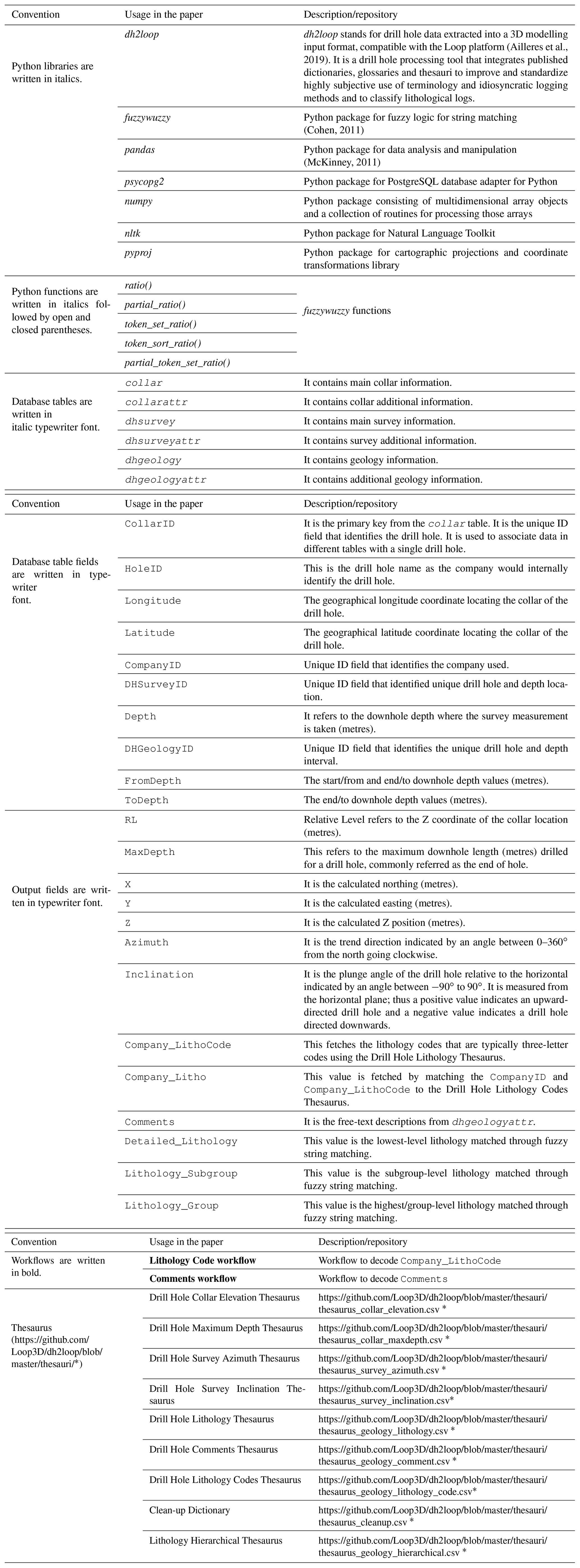
* last access: 30 September 2021.
A2 Installation and dependencies
Installing dh2loop can be done by cloning the GitHub repository with $ git clone https://github.com/Loop3D/dh2loop.git (last access: 30 September 2021) and then manually installing it by running the Python setup script in the repository: $ Python setup.py install.
It primarily depends on a number of external open-source libraries:
-
fuzzywuzzy (https://github.com/seatgeek/fuzzywuzzy), which uses fuzzy logic for string matching (Cohen, 2011)
-
pandas (https://pandas.pydata.org/, last access: 30 September 2021) for data analysis and manipulation (McKinney, 2011)
-
psycopg2 (https://pypi.org/project/psycopg2/, last access: 30 September 2021), a PostgreSQL database adapter for Python (Gregorio and Varrazzo, 2018)
-
numpy (https://github.com/numpy/numpy, last access: 30 September 2021)
-
nltk (https://github.com/nltk/nltk, last access: 30 September 2021), the Natural Language Toolkit, a suite of open-source Python modules, datasets, and tutorials supporting research and development in natural language processing (Loper and Bird, 2002).
-
pyproj (https://github.com/pyproj4/pyproj, last access: 30 September 2021), Python interface to PROJ (cartographic projections and coordinate transformations library).
Code describing basic drill hole operations, such as de-surveying (process of translating collar (location) and survey data (azimuth, inclination, length) of drill holes into XYZ coordinates in order to define its 3D geometry of the non-vertical borehole), is heavily inspired by the pyGSLIB drill hole module (Martínez-Vargas, 2016). The pyGSLIB drill hole module is re-written into Python to make it more compact with less dependencies and to tailor it to the data extraction output.
A3 Documentation
dh2loop's documentation provides a general overview over the library and multiple in-depth tutorials. The tutorials are provided as Jupyter Notebooks, which will provide the convenient combination of documentation and executable script blocks in one document. The notebooks are part of the repository and located in the notebooks folder. See http://jupyter.org/ (last access: 30 September 2021) for more information on installing and running Jupyter Notebooks.
A4 Jupyter notebooks
Jupyter notebooks are provided as part of the online documentation. These notebooks can be executed in a local Python environment (if the required dependencies are correctly installed). In addition, static versions of the notebooks can currently be inspected directly on the github repository web page or through the use of nbviewer.
-
WAMEX Interactive report downloads (https://github.com/Loop3D/dh2loop/blob/master/notebooks/0_WAMEX_Downloads_Interactive.ipynb, last access: 30 September 2021)
-
Exporting and Text Parsing of Drillhole Data From PostgreSQL database (https://github.com/Loop3D/dh2loop/blob/master/notebooks/1_Exporting_and_Text_Parsing_of_Drillhole_Data_From_PostgreSQL.ipynb, last access: 30 September 2021)
-
Exporting and Text Parsing of Drillhole Data Demo (https://github.com/Loop3D/dh2loop/blob/master/notebooks/2_Exporting_and_Text_Parsing_of_Drillhole_Data_Demo.ipynb, last access: 30 September 2021)
-
Harmonizing Drillhole data (https://github.com/Loop3D/dh2loop/blob/master/notebooks/3_Harmonizing_Drillhole_Data.ipynb, last access: 30 September 2021).
B1 Collar extraction
The collar extraction workflow (Fig. B3) fetches the CollarID, HoleID, Longitude and
Latitude information from the collar table (Fig. B3a, red), while the corresponding RL
and MaxDepth values are fetched from the collarattr table using the Drill Hole Collar
Elevation Thesaurus (Fig. B3b, blue) and Drill Hole Maximum Depth Thesaurus (Fig. B3c,
orange). With the minimum input of a region of interest, the dh2loop library exports
a comma-separated values file (CSV) listing the drill holes in the area with
the following information:
-
CollarID: theCollarIDfor a drill hole is identical in all tables in order for data to be associated with that drill hole. -
HoleID: this is the drill hole name, as the company would internally identify the drill hole. -
LongitudeandLatitude: both values are expressed in WGS 1984 lat/long (EPSG:4326). -
Relative level (
RL): we useRLhere to refer to elevations of survey points with reference to the mean sea level. This definition ofRLis equivalent to the elevation values used in digital elevation models (DEMs). This value is extracted by using the Drill Hole Collar Elevation Thesaurus to filter the values referring to relative level. More than one value can be fetched due to duplicate company submissions or multiple elevation measurements, in which case the code retains the value with most decimal places assuming that higher precision corresponds to better accuracy. If no elevation values are fetched from the database the entire record is skipped. Non-numeric values are also ignored. -
Maximum depth (
MaxDepth): this value is extracted by using the Drill Hole Maximum Depth Thesaurus. Due to duplicate company submissions, there can be more than one value fetched. Since there is no submission date information, the code takes the value with the largest value assuming it is the latest submission. -
Calculated
X,Yvalues of projected coordinates: these values are commonly calculated and used to be able to plot the drill hole in a metric system to be able to accurately display and measure distance within and between drill holes. The projection system used in the calculation is based on the input specified in the configuration file.
The extraction of the collar data for YSGB resulted in a collar file with 68 729
drill holes. This information is extracted from the collar table with 73 881 drill
holes with 769 981 rows of information from collarattr. It includes the location of
the collar both in geographic and projected coordinated systems, relative
level (RL) and maximum depth (MaxDepth). A total of 136 100 records for RL
is retrieved from the database, 1526 of which are disregarded: 846 records
for having an RL value greater than 10 000 m and 680 non-numeric
records. These discarded values are retrieved from the attribute column
“RL_Local”. In spite of it being an isolated issue for
“RL_Local”, the attribute column is retained as it retrieves sensible values for other companies. The discarded values are
limited to data from two companies (4085, 4670) for RL attribute columns
“TD” and “DEPTH”. A total of 58 706 records for MaxDepth are retrieved
from the database, 58 642 of which are extracted as is, while 64 entries are
disregarded for having a value of −999. The discarded values come from eight companies. Null values are disregarded and absent RL or MaxDepth values. The
“clean” collar export file contains at least either a value for RL or MaxDepth. The reasoning behind keeping records with at least one of the two fields is that there are other ways to extract RL or MaxDepth from the
database. RL values can be extracted from digital terrain models and
MaxDepth values can be taken for the largest ToDepth values from the other
tables. In total 93 % of the available collar data in the area is extracted
successfully. This can be improved by implementing alternative ways of retrieving RL and MaxDepth values. For example, if no RL values are fetched
from the database, they could be fetched from open-source digital terrain
models (DTMs) or the SRTM (Shuttle Radar Topography Mission). As for missing
MaxDepth values, the maximum ToDepth values in the survey or interval
tables could be used.
B2 Survey extraction
The survey extraction workflow (Fig. B4) fetches the DHSurveyID, CollarID and Depth
information from the dhsurvey table (Fig. B4a, red), while the corresponding azimuth and
inclination values are fetched from the dhsurveyattr table using the Drill Hole Survey
Azimuth Thesaurus (Fig. B4b, blue) and Drill Hole Survey Inclination Thesaurus (Fig. B4c,
orange).With the same inputs defined in the configuration file, the
dh2loop library outputs a survey CSV file containing the following information:
CollarID, Depth, Azimuth, Inclination and Calculated X, Y, Z values. The
workflow accommodates underground holes drilled upwards as long as the
metadata and data appropriately describe them as such. For all properties,
all non-numeric values are ignored. For Depth, negative values are replaced
by their absolute value. This assumption is made as some drill holes have
negative depth information and it is technically not possible to have a
negative length. This is done by some companies to denote that the depth
measure is going upwards (usually for underground probing drill holes)
rather than downwards. For Azimuth, the code fetches values between 0–360∘, thus ignoring values greater than 360. Values between −360 to 0 are
assumed to be anticlockwise from the north. If there is no survey
information for a drill hole present in collar, the Azimuth value is set to
0. The X, Y, Z, values are calculated using the minimum curvature basing the
code on the pyGSLIB drill hole module.
For the survey extraction, the dhsurvey table contained 146 713 survey depth
intervals (from 45 708 drill holes) with a corresponding 850 507 entries of
supplementary survey information in dhsurveyattr. Survey extraction in YSGB resulted in
126 669 pieces of survey depth information across 45 708 drill holes with azimuth
(−52.5 to 359) and inclination measurements (0–90) for each depth interval.
A total of 517 592 records for Azimuth are retrieved from the database. In total, 77
Azimuth values greater than 360 are retrieved and thus disregarded. In total, 152
values are non-numeric values and are also disregarded. These discarded
values involved 228 holes across 10 companies. A value of 0 is assigned to
missing Azimuth values. A total of 118 223 records for Inclination are
fetched from the database, 118 138 of which are extracted as is, while 95
entries are disregarded for having a value greater than 90. A values of −90
is assigned as the default for inclination. The discarded values correspond
to 94 drill holes across five companies. The survey extraction rate of 86 %
is fairly good. dh2loop ensures that the Azimuth and Inclination values are
sensible measurements before including them in the extracted output file.
An improvement that could be implemented is to run an assessment on the
deflection angles for each drill hole and flag intervals with unrealistic
deflection angles.
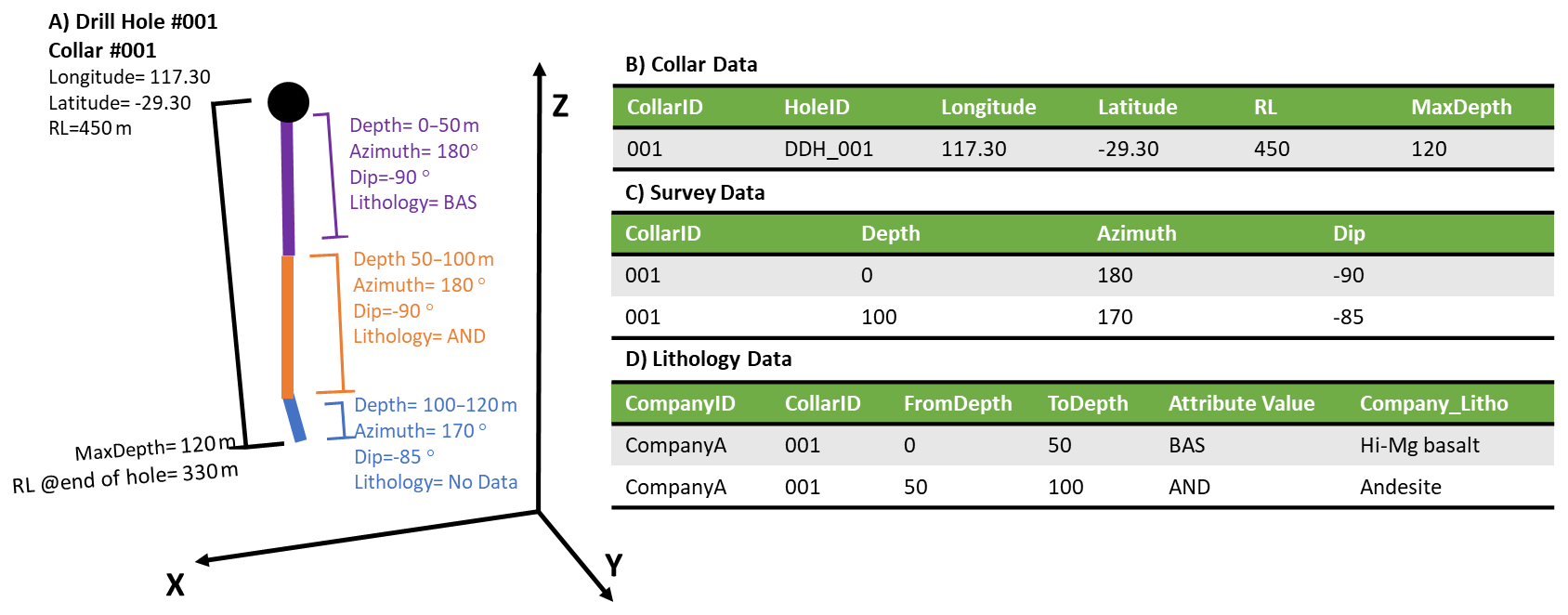
Figure B1Simplified example of a drill hole (1.A) and its corresponding interval
tables collar (1.B), survey (1.C) and lithology (1.D). The black circle
denotes the collar location of the drill hole which is obtained from a
collar table (1.B). The purple line represents the first downhole interval
taking its deviation data from the survey table (1.C) and the lithology
information from the lithology table (1.D). The same applies for the second
interval (orange line) and the third interval (blue line). The orange line
follows the same trajectory as the first interval as it uses the same entry
in the survey table (1.C). The blue line has no lithology data as this
information is not present in the lithology table (1.D). The MaxDepth denotes the total drill length (1.B).
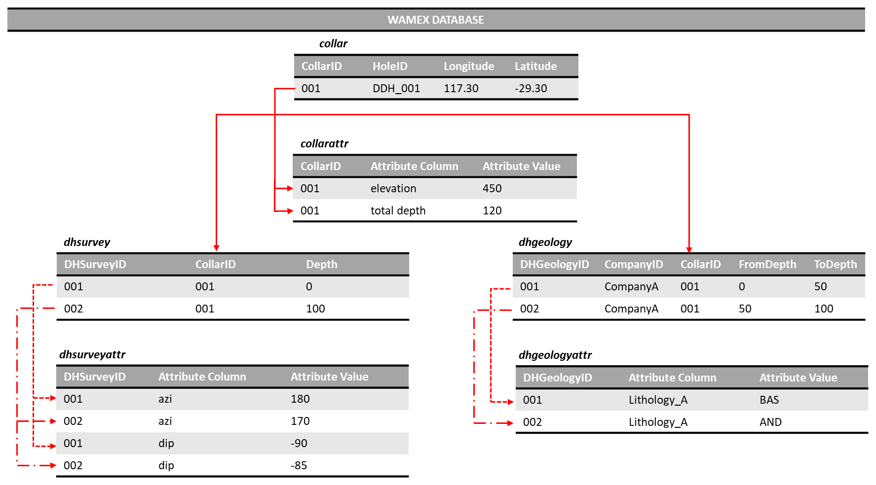
Figure B2Simplified WAMEX database schema showing the one-to-many relationship
between the collar table and the collarattr table (red solid line). collarattr stores other attributes
that describe each unique drill hole, such as maximum depth and elevation.
The figure also shows the relationship between the collar table and the other
interval tables such as dhsurvey, dhsurveyattr, dhgeology and dhgeologyattr. The deviation of the drill hole is stored in a
table, dhsurvey, with a primary key (DHSurveyID) that refers to each unique depth of
a drill hole. This primary key has a many-to-one relationship with collar,
as there are multiple depth measurements for each drill hole. Furthermore,
dhsurvey also has a one-to-many relationship with the table dhsurveyattr, which stores additional
attribute information regarding survey, such as Azimuth and Inclination readings. The example shows the relationship between tables for the first
(red dashed line) and second interval (red dashed–dot line). Each drill hole
in the WAMEX database is identified by its geographic coordinates and a
unique ID (CollarID) in the collar table. The drill hole 3D geometry is
described in the survey tables (dhsurvey, dhsurveyattr). This similar relationship is maintained
with interval tables, except that the primary key (e.g. DHGeologyID) is used
to refer a unique downhole interval rather than a depth measurement. For
lithological information, we refer to tables dhgeology and dhgeologyattr. dhgeologyattr contains
information such as rock names and free-text descriptions, while dhgeology provides
information on which hole and interval depth those data refer to. This
information can be joined and extracted through SQL (Structured Query
Language) queries.

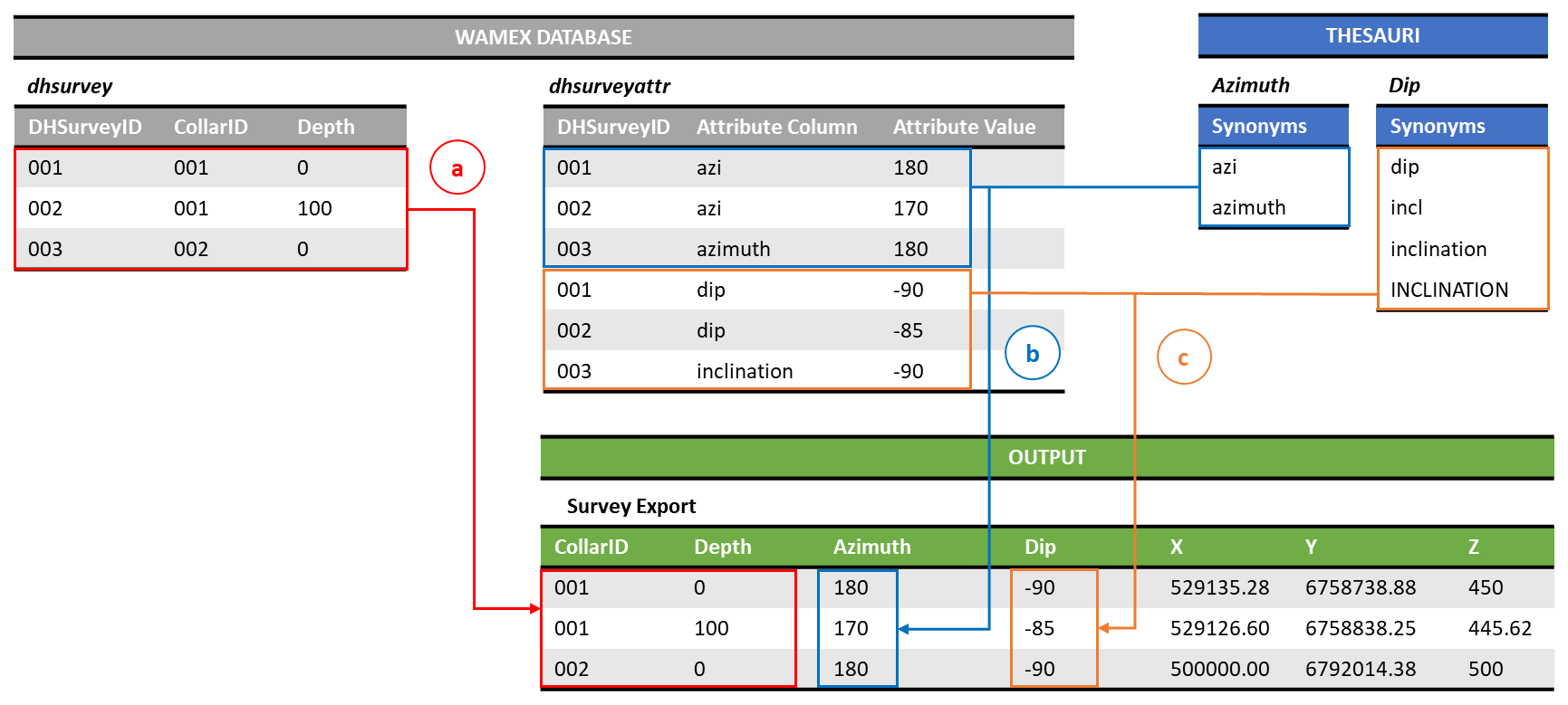
dh2loop is a free, open-source Python library licensed under the MIT License. It is hosted on the GitHub repository (https://github.com/Loop3D/dh2loop) and can be cited as http://doi.org/10.5281/zenodo.4043568 (Joshi et al., 2020).
MJ contributed the original idea, which led to further developed by RJ. KM developed the code. MJ, ML and GP provided guidance and direction in the research. RJ prepared the paper with contributions from all co-authors. Lastly, MJ supervised the entire process.
The authors declare that they have no conflict of interest.
Publisher’s note: Copernicus Publications remains neutral with regard to jurisdictional claims in published maps and institutional affiliations.
The research was carried out while the first author was in receipt of a Scholarship for International Research Fees (Australian Government Research Training Program Scholarship) and an Automated 3D Geology Modelling PhD Scholarship (University Postgraduate Award) at the University of Western Australia. We acknowledge the support from the ARC-funded Loop: Enabling Stochastic 3D Geological Modelling consortia (LP170100985) and DECRA (DE190100431). The work has been supported by the Mineral Exploration Cooperative Research Centre, whose activities are funded by the Australian Government's Cooperative Research Centre Program. This is MinEx CRC Document 2021/49. We would also like to acknowledge Tim Ivanic for his input on the geology of the Yalgoo–Singleton greenstone belt.
This research has been supported by the Australian Research Council (grant nos. LP170100985 and DE190100431).
This paper was edited by Andrew Wickert and reviewed by Matt Hall, Ignacio Fuentes, and one anonymous referee.
Ailleres, L., Jessell, M., de Kemp, E., Caumon, G., Wellmann, F., Grose, L., Armit, R., Lindsay, M., Giraud, J., Brodaric, B., Harrison, M., and Courrioux, G.: Loop – Enabling 3D stochastic geological modelling, ASEG Extended Abstracts, 2019, 1–3, https://doi.org/10.1080/22020586.2019.12072955, 2019.
Anand, R. R. and Butt, C. R. M.: A guide for mineral exploration through the regolith in the Yilgarn Craton, Western Australia, Aust. J. Earth Sci., 57, 1015–1114, https://doi.org/10.1080/08120099.2010.522823, 2010.
Arabjamaloei, R., Edalatkha, S., Jamshidi, E., Nabaei, M., Beidokhti, M., and Azad, M.: Exact Lithologic Boundary Detection Based on Wavelet Transform Analysis and Real-Time Investigation of Facies Discontinuities Using Drilling Data, Pet. Sci. Technol., 29, 569–578, https://doi.org/10.1080/10916460903419206, 2011.
Barley, M. E., Brown, S. J. A., Krapez, B., and Kositcin, N.: Physical volcanology and geochemistry of a Late Archaean volcanic arc: Kurnalpi and Gindalbie Terranes, Eastern Goldfields Superterrane, Western Australia, Precambrian Res., 161, 53–76, https://doi.org/10.1016/j.precamres.2007.06.019, 2008.
Chace, F. M.: Abbreviations in field and mine geological mapping, Econ. Geol., 51, 712–723, 1956.
Cockbain, A. E.: Regolith geology of the Yilgarn Craton – Introduction, Aust. J. Earth Sci., 49, 1–1, https://doi.org/10.1046/j.1440-0952.2002.00913.x, 2002.
Cohen, A.: FuzzyWuzzy: Fuzzy string matching in python, ChairNerd Blog, available at: http://chairnerd.seatgeek.com/fuzzywuzzy-fuzzy-string-matching-in-python/ (last accessed: 29 September 2021), 2011.
Culshaw, M. G.: From concept towards reality: developing the attributed 3D geological model of the shallow subsurface, Q. J. Eng. Geol. Hydroge., 38, 231–284, https://doi.org/10.1144/1470-9236/04-072, 2005.
Eggleton, R. A.: The regolith glossary, Cooperative Centre for Landscape Evolution and Mineral Exploration, 8, 144 pp., National Capital Printing, Canberra, Australia, 2001.
Emelyanova, I., Pervukhina, M., Clennell, M., and Dyt, C.: Unsupervised identification of electrofacies employing machine learning, 79th EAGE Conference and Exhibition 2017, Paris, France, 12–16 June 2017, EAGE, 2017.
Erkan, G. and Radev, D. R.: LexRank: Graph-based lexical centrality as salience in text summarization, J. Artif. Intell. Res., 22, 457–479, https://doi.org/10.1613/jair.1523, 2004.
Fuentes, I., Padarian, J., Iwanaga, T., and Vervoort, R. W.: 3D lithological mapping of borehole descriptions using word embeddings, Comput. Geosci., 141, 104516, https://doi.org/10.1016/j.cageo.2020.104516, 2020.
Gillespie, M. and Styles, M.: BGS rock classification scheme, Volume 1, Classification of igneous rocks, Keyworth, Nottingham, British Geological Survey, 31 pp., RR/99/006, 1999.
Gonzalez, J., Rodrigues, P., and Cohen, A.: Fuzzywuzzy: Fuzzy string matching in python, available at: https://github.com/seatgeek/fuzzywuzzy (last access: 30 September 2021), 2017.
Gregorio, F. D. and Varrazzo, D.: psycopg2, available at: http://initd.org/psycopg/docs/ (Stand: 17 June 2021) (last access: 30 September 2021), 2018.
Griffin, R. E.: When are Old Data New Data?, GeoResJ, 6, 92–97, https://doi.org/10.1016/j.grj.2015.02.004, 2015.
Groves, D. I., Goldfarb, R. J., Knox-Robinson, C. M., Ojala, J., Gardoll, S., Yun, G. Y., and Holyland, P.: Late-kinematic timing of orogenic gold deposits and significance for computer-based exploration techniques with emphasis on the Yilgarn Block, Western Australia, Ore Geol. Rev., 17, 1–38, https://doi.org/10.1016/S0169-1368(00)00002-0, 2000.
Hall, M. and Keppie, F.: Striplog: new open source software for handling and analysing discontinuous and qualitative data, oral paper at the Atlantic Geoscience Society Colloquium, Truro, Nova Scotia, Canada, 5–6 February 2016.
Hallsworth, C. R. and Knox, R.: BGS rock classification scheme, Volume 3, classification of sediments and sedimentary rocks, British Geological Survey, Keyworth, Nottingham, 24 pp., RR/99/003, 1999.
Higgins, R. F. and Mehta, S.: SeatGeek, Harvard Business School Case 819-013, October 2018.
Hill, E. J., Robertson, J., and Uvarova, Y.: Multiscale hierarchical domaining and compression of drill hole data, Comput. Geosci., 79, 47–57, https://doi.org/10.1016/j.cageo.2015.03.005, 2015.
Hill, E. J., Pearce, M. A., and Stromberg, J. M.: Improving Automated Geological Logging of Drill Holes by Incorporating Multiscale Spatial Methods, Math. Geosci., 53, 21–53, https://doi.org/10.1007/s11004-020-09859-0, 2020.
Jallan, Y., Brogan, E., Ashuri, B., and Clevenger, C. M.: Application of Natural Language Processing and Text Mining to Identify Patterns in Construction-Defect Litigation Cases, Journal of Legal Affairs and Dispute Resolution in Engineering and Construction, 11, 04519024, https://doi.org/10.1061/(Asce)La.1943-4170.0000308, 2019.
Joshi, R., Madaiah, K., and Jessell, M.: Loop3D/dh2loop: dh2loop first release (v1.0.0), Zenodo [data set], https://doi.org/10.5281/zenodo.4043568, 2020.
Kumari, S., Mohan, A., and Saberwal, G.: Hidden duplicates: 10s or 100s of Indian trials, registered with ClinicalTrials.gov, have not been registered in India, as required by law, PLoS One, 15, e0234925, https://doi.org/10.1371/journal.pone.0234925, 2020.
Lark, R. M., Thorpe, S., Kessler, H., and Mathers, S. J.: Interpretative modelling of a geological cross section from boreholes: sources of uncertainty and their quantification, Solid Earth, 5, 1189–1203, https://doi.org/10.5194/se-5-1189-2014, 2014.
Le Vaillant, M., Hill, J., and Barnes, S. J.: Simplifying drill-hole domains for 3D geochemical modelling: An example from the Kevitsa Ni-Cu-(PGE) deposit, Ore Geol. Rev., 90, 388–398, https://doi.org/10.1016/j.oregeorev.2017.05.020, 2017.
Levenshtein, V.: Leveinshtein distance, available at: http://en.wikipedia.org/wiki/Levenshtein_distance (last access: 30 September 2021), 1965.
Lin, C.-Y. and Hovy, E.: Automatic evaluation of summaries using N-gram co-occurrence statistics, in: Proceedings of the 2003 Human Language Technology Conference of the North American Chapter of the Association for Computational Linguistics, Edmonton, Canada, May–June 2003, 71–78, https://doi.org/10.3115/1073445.1073465, 2003.
Lindsay, M.: Geological Interpretation of Geophysics Support from Machine Learning of Drillcore, in: Geological Survey of Western Australia Open Day 2019, Perth, Australia, available at: https://geodocs.dmirs.wa.gov.au/Web/documentlist/16/DirectLink/GeologicalInterpretationGS (last access: 30 September 2021), 2019.
Liu, K., Hogan, W. R., and Crowley, R. S.: Natural Language Processing methods and systems for biomedical ontology learning, J. Biomed. Inform., 44, 163–179, https://doi.org/10.1016/j.jbi.2010.07.006, 2011.
Liu, T. and Guo, J.: Text similarity computing based on standard deviation, in: Advances in Intelligent Computing, edited by: Huang, D. S., Zhang, X. P., and Huang, G. B., International Conference on Intelligent Computing 2005, Lecture Notes in Computer Science, vol. 3644, 456–464, https://doi.org/10.1007/11538059_48, 2005.
Loper, E. and Bird, S.: NLTK: the natural language toolkit, arXiv [preprint], arXiv:cs/0205028, 17 May 2002.
Martínez-Vargas, A.: PyGSLIB [online], Python 2.7 package, Opengeostat Consulting, available at: https://github.com/opengeostat/pygslib (last access: 30 September 2021), 2016.
McKinney, W.: pandas: a foundational Python library for data analysis and statistics, Python for High Performance and Scientific Computing, 14, 1–9, 2011.
McMillan, A. and Powell, J.: British Geological Survey Rock Classification Scheme, Volume 4: The Classification of Artificial (man made) Ground and Natural Superficial Deposits: Applications to Geological Maps and Datasets in the UK, British Geolgoical Survey Research Report, RR 99-04, 1999.
Miles, A. and Bechhofer, S.: SKOS simple knowledge organization system reference, W3C recommendation, 18, World Wide Web Consortium, available at: http://www.w3.org/TR/skos-reference/ (last access: 30 September 2021), 2009.
Müller, T., Cotterell, R., Fraser, A., and Schütze, H.: Joint lemmatization and morphological tagging with lemming, in: Proceedings of the 2015 Conference on Empirical Methods in Natural Language Processing, Association for Computational Linguistics, Lisbon, Portugal, 2268–2274, https://doi.org/10.18653/v1/D15-1272, 2015.
Myers, J.: Precambrian Tectonic History of the West Australian Craton and Adjacent Orogens, Annu. Rev. Earth Pl. Sc., 21, 453–485, https://doi.org/10.1146/annurev.ea.21.050193.002321, 1993.
Okuda, T., Tanaka, E., and Kasai, T.: A method for the correction of garbled words based on the Levenshtein metric, IEEE T. Comput., 100, 172–178, 1976.
Otter, D. W., Medina, J. R., and Kalita, J. K.: A Survey of the Usages of Deep Learning for Natural Language Processing, IEEE T. Neural Net. Lear., 32, 604–624, https://doi.org/10.1109/TNNLS.2020.2979670, 2020.
Padarian, J. and Fuentes, I.: Word embeddings for application in geosciences: development, evaluation, and examples of soil-related concepts, SOIL, 5, 177–187, https://doi.org/10.5194/soil-5-177-2019, 2019.
Park, S. H., Ryu, K. H., and Gilbert, D.: Fast similarity search for protein 3D structures using topological pattern matching based on spatial relations, Int. J. Neural. Syst., 15, 287–296, https://doi.org/10.1142/S0129065705000244, 2005.
Qiu, Q., Xie, Z., Wu, L., and Tao, L.: Dictionary-Based Automated Information Extraction From Geological Documents Using a Deep Learning Algorithm, Earth and Space Science, 7, e2019EA000993, https://doi.org/10.1029/2019ea000993, 2020.
Ralph, J..: Mindat.org, available at: https://www.mindat.org/min-50468.html, last access: 30 September 2021.
Raymond, O., Duclaux, G., Boisvert, E., Cipolloni, C., Cox, S., Laxton, J., Letourneau, F., Richard, S., Ritchie, A., and Sen, M.: GeoSciML v3.0 – a significant upgrade of the CGI-IUGS geoscience data model, EGU General Assembly 2012, Vienna, Austria, 22–27 April, 2012, 2711, available at: https://ui.adsabs.harvard.edu/abs/2012EGUGA..14.2711R (last access: 30 September 2021), 2012.
Recasens, M., Danescu-Niculescu-Mizil, C., and Jurafsky, D.: Linguistic models for analyzing and detecting biased language, in: Proceedings of the 51st Annual Meeting of the Association for Computational Linguistics, Sofia, Bulgaria, August 2013, Volume 1: Long Papers, 1650–1659, available at: https://aclanthology.org/P13-1162.pdf (last access: 30 September 2021), 2013.
Richard, S. M. and CGI Interoperability Working Group: GeoSciML – a GML application for geoscience information interchange, Digital Mapping Techniques 2007, Workshop Proceedings: U.S. Geological Survey, 1285, 47–59, 2007.
Riganti, A., Farrell, T. R., Ellis, M. J., Irimies, F., Strickland, C. D., Martin, S. K., and Wallace, D. J.: 125 years of legacy data at the Geological Survey of Western Australia: Capture and delivery, GeoResJ, 6, 175–194, https://doi.org/10.1016/j.grj.2015.02.015, 2015.
Rivera-Quiroz, F. A. and Miller, J.: Extracting Data from Legacy Taxonomic Literature: Applications for planning field work, Biodiversity Information Science and Standards, 3, e37082, https://doi.org/10.3897/biss.3.37082, 2019.
Robertson, S.: BGS rock classification scheme, Volume 2, Classification of metamorphic rocks, British Geological Survey Research Report, RR 99–02, 24 pp., 1999.
Rosenbaum, M. S., McMillan, A. A., Powell, J. H., Cooper, A. H., Culshaw, M. G., and Northmore, K. J.: Classification of artificial (man-made) ground, Eng. Geol., 69, 399–409, https://doi.org/10.1016/S0013-7952(02)00282-X, 2003.
Ross, P. S., Bourke, A., and Fresia, B.: A multi-sensor logger for rock cores: Methodology and preliminary results from the Matagami mining camp, Canada, Ore Geol. Rev., 53, 93–111, https://doi.org/10.1016/j.oregeorev.2013.01.002, 2013.
Rothwell, R. G. and Rack, F. R.: New techniques in sediment core analysis: an introduction, New Techniques in Sediment Core Analysis, The Geological Society of London, 267, 1–29, https://doi.org/10.1144/Gsl.Sp.2006.267.01.01, 2006.
Schetselaar, E. M. and Lemieux, D.: A drill hole query algorithm for extracting lithostratigraphic contacts in support of 3D geologic modelling in crystalline basement, Comput. Geosci., 44, 146–155, https://doi.org/10.1016/j.cageo.2011.10.015, 2012.
Simons, B., Boisvert, E., Brodaric, B., Cox, S., Duffy, T. R., Johnson,B. R., Laxton, J. L., and Richard, S.: GeoSciML: enabling the exchange of geological map data, ASEG Extended Abstracts, 2006, 1–4, https://doi.org/10.1071/ASEG2006ab162, 2006.
Smith, M. J., Keesstra, S., and Rose, J.: Use of legacy data in geomorphological research, GeoResJ, 6, 74–80, https://doi.org/10.1016/j.grj.2015.02.008, 2015.
Vearncombe, J., Conner, G., and Bright, S.: Value from legacy data, T. I. Min. Metall. B, 125, 231–246, https://doi.org/10.1080/03717453.2016.1190442, 2016.
Vearncombe, J., Riganti, A., Isles, D., and Bright, S.: Data upcycling, Ore Geol. Rev., 89, 887–893, https://doi.org/10.1016/j.oregeorev.2017.07.009, 2017.
Wang, C. and Ma, X.: Text Mining to Facilitate Domain Knowledge Discovery, in: Text Mining-Analysis, Programming and Application, IntechOpen, https://doi.org/10.5772/intechopen.85362, 2019.
Wilbur, W. J. and Sirotkin, K.: The Automatic Identification of Stop Words, J. Inf. Sci., 18, 45–55, https://doi.org/10.1177/016555159201800106, 1992.
Zhou, C. Y., Ouyang, J. W., Ming, W. H., Zhang, G. H., Du, Z. C., and Liu, Z.: A Stratigraphic Prediction Method Based on Machine Learning, Appl. Sci.-Basel, 9, 3553, https://doi.org/10.3390/app9173553, 2019.
Zhou, Q., Liu, H. H., Bodvarsson, G. S., and Oldenburg, C. M.: Flow and transport in unsaturated fractured rock: effects of multiscale heterogeneity of hydrogeologic properties, J. Contam. Hydrol., 60, 1–30, https://doi.org/10.1016/s0169-7722(02)00080-3, 2003.
Zhu, G., Gao, M., Kong, F., and Li, K.: Application of Logging While Drilling Tool in Formation Boundary Detection and Geo-steering, Sensors (Basel), 19, 2754, https://doi.org/10.3390/s19122754, 2019.
- Abstract
- Introduction
- dh2loop drill hole data extraction
- Case study: Yalgoo–Singleton greenstone belt
- Discussion
- Conclusions
- Appendix A: dh2loop package information
- Appendix B: Collar and survey data extraction
- Code and data availability
- Author contributions
- Competing interests
- Disclaimer
- Acknowledgements
- Financial support
- Review statement
- References