Spatial agents for geological surface modelling

Increased availability and use of 3D-rendered geological models have provided society with predictive capabilities, supporting natural resource assessments, hazard awareness, and infrastructure development. The Geological Survey of Canada, along with other such institutions, has been trying to standardize and operationalize this modelling practice. Knowing what is in the subsurface, however, is not an easy exercise, especially when it is difficult or impossible to sample at greater depths. Existing approaches for creating 3D geological models involve developing surface components that represent spatial geological features, horizons, faults, and folds, and then assembling them into a framework model as context for downstream property modelling applications (e.g. geophysical inversions, thermo-mechanical simulations, and fracture density models). The current challenge is to develop geologically reasonable starting framework models from regions with sparser data when we have more complicated geology. This study explores the problem of geological data sparsity and presents a new approach that may be useful to open up the logjam in modelling the more challenging terrains using an agent-based approach.

Semi-autonomous software entities called spatial agents can be programmed to perform spatial and property interrogation functions, estimations and construction operations for simple graphical objects, that may be usable in building 3D geological surfaces. These surfaces form the building blocks from which full geological and topological models are built and may be useful in sparse-data environments, where ancillary or a priori information is available. Critical in developing natural domain models is the use of gradient information. Increasing the density of spatial gradient information (fabric dips, fold plunges, and local or regional trends) from geologic feature orientations (planar and linear) is the key to more accurate geologic modelling and is core to the functions of spatial agents presented herein. This study, for the first time, examines the potential use of spatial agents to increase gradient constraints in the context of the Loop project (https://loop3d.github.io/, last access: 1 October 2021​​​​​​​) in which new complementary methods are being developed for modelling complex geology for regional applications. The spatial agent codes presented may act to densify and supplement gradient as well as on-contact control points used in LoopStructural (https://www.github.com/Loop3d/LoopStructural, last access: 1 October 2021) and Map2Loop (https://doi.org/10.5281/zenodo.4288476, de Rose et al., 2020).

Spatial agents are used to represent common geological data constraints, such as interface locations and gradient geometry, and simple but topologically consistent triangulated meshes. Spatial agents can potentially be used to develop surfaces that conform to reasonable geological patterns of interest, provided that they are embedded with behaviours that are reflective of the knowledge of their geological environment. Initially, this would involve detecting simple geological constraints: locations, trajectories, and trends of geological interfaces. Local and global eigenvectors enable spatial continuity estimates, which can reflect geological trends, with rotational bias, using a quaternion implementation. Spatial interpolation of structural geology orientation data with spatial agents employs a range of simple nearest-neighbour to inverse-distance-weighted (IDW) and quaternion-based spherical linear rotation interpolation (SLERP) schemes. This simulation environment implemented in NetLogo 3D is potentially useful for complex-geology–sparse-data environments where extension, projection, and propagation functions are needed to create more realistic geological forms.

1 Introduction

The major challenge that this paper is trying to address is the breakdown in achieving geologically realistic model results from sparse data in more complicated geological scenarios when using the existing methods and algorithms. This is no doubt a problem in other modelling domains, but it is an acute issue in geological applications, where access to data in the subsurface is often extremely expensive, terrain access is prohibitive, or the depth of investigation is too extreme for direct sampling and must rely on coarser geophysical methods that often do not adequately image the features being modelled. This paper explores the use of extension, propagation, and cohesion methods, which can be considered part of “swarm” technology, using spatial agents in an attempt to deal with this challenge.

Geological modelling covers a wide range of applications and domains from thermo-mechanical modelling (Cloetingh et al., 2013) to basin analysis (Barrett et al., 2018), mineral potential estimation (Skirrow et al., 2019) in 3D (Hu et al., 2020; Sprague et al., 2006), and even 4D applications (Parquer et al., 2020; White, 2013). Herein, we focus on the starting framework model, the stratigraphic and structural surface model that provides the initial context for these more downstream property-embedded modelling efforts. Generally, these geological models can be represented as BREP (boundary representation) models (Pellerin et al., 2017; Caumon et al., 2009), but recently, many of these have been defined through implicit derived surfaces with topologically encoded volumes (Grose et al., 2021; de la Varga et al., 2019; Wellmann et al., 2019; Grose et al., 2017; Laurent et al., 2016; Hillier et al., 2014; Frank et al. 2007; Courrioux et al., 2001; Lajaunie et al., 1997). In each case, the accuracy of the BREP and/or implicit surface model features, such as horizons, folds, or faults, are dependent on the quality of the geological input data that are available as well as on the algorithms and methods used to build them (Wellmann and Caumon, 2018; MacCormack and Eyles, 2012).

Existing methods applied to the combined sparse-data–complex-geology scenario will tend to produce holes, gaps, and feature drop-outs away from control data as well as arbitrary horizon thickness changes that combine to give a geologically unreasonable bubblegum look to these models (Fig. 1). Current methods in sparse-data configurations tend to be biased towards these unrealistic geometries using radial-based kernel functions, optimized for local smoothness in order to achieve a mathematical solution (Hillier et al., 2021, 2014). This often comes at the price of geological realism (Hillier et al., 2021; MacCormack and Eyles, 2012). Is it possible that, with a new approach, geological features could be more realistically modelled by using spatial agents to “fill the gaps” in the process?

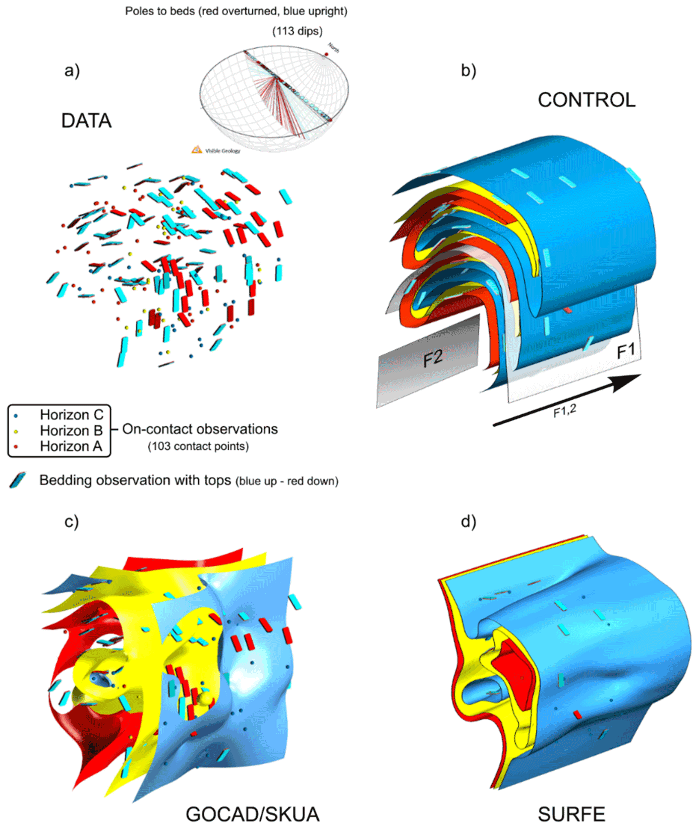
Figure 1 Comparison of synthetic geological 3D models of classic Ramsay type-3 interference folds (Ramsay, 1967, 1962), with identical data. (a) Uniaxial dip data, with local opposing tops, represented on an equal-angle Wulff plot (https://app.visiblegeology.com/stereonet.html, last access: 1 October 2021). (b) Control model developed with SPARSE (de Kemp et al., 2004), with F1–F2 horizontal, north-trending hinges, and (c) implicit surface models with GOCAD/SKUA (Jayr et al., 2008) and (d) SURFE (Hillier et al., 2014). Figure adapted from Hillier et al. (2016).

Section 1 provides an overview, context, and review for the current study, surveying various application domains with an eye toward natural and more specific Earth sciences agent applications. Section 2 outlines the use of spatial agents for structural geology. A summary of current geological surface modelling approaches is given, with argumentation that highlights the need for new approaches, particularly when data are sparse and geology is more complex. Highlighted are mechanisms for using structural constraints, inter-agent communication, and characterization of required agent behaviours. A summary of the critical intrinsic properties of spatial agents that may aid in future research in this area is also given. In Sect. 3, several spatial agent demos are used to represent simple contact surfaces as agent-constructed triangular meshes, fold closures, and simulations of unmeshed structural swarms from sparse points. There are six main programs, each highlighting critical functionality that will be required should structural agents be developed into a more complete geomodelling system in the future. Lastly, Sect. 4 provides a discussion on how structural agents could be applied as well as some final conclusions from the study.

1.1 Agent challenge

Spatial agents are virtual spatial entities that have the freedom to interact with each other and their environment, which can include various domain data, in order to solve a well-defined problem – for example, to predict the growth of an urban centre, an ant hill, or the course of a meandering river system under variable rainfall and soil conditions. Some of the core characteristics of spatial agents could potentially be used to essentially “grow” features away from the control data, keeping them intact while extending and respecting regional gradient information. In a sense, this is similar to how the human mind might fill gaps through geological interpretation of a map or cross section.

The Loop effort is attempting to address this ongoing challenge (Ailleres et al., 2019) that tends to present itself when geology becomes more complicated, using more elaborate geo-histories, for example, geo-histories with early cryptic sedimentary and volcanic depositional cycles as well as a spectrum of brittle to deeper crustal deformation events, and through masking metamorphic processes. Geo-histories with overprinting intrusive events, from thin dyke swarms to consuming batholithic intrusions, can also completely erase all macroscopic evidence of earlier processes. The challenge is most acute when the data required to accurately model these scenarios are quite limited, such as in inland frontier zones, where most of our data are only at ground surface, interpreted from remote sensing images, or sparingly at depth, with clustered spatially biased drill holes near mineralized zones. These regions may have been surveyed with geophysical instruments, and the data used to derive models represent at-depth rock property distributions for density and magnetic susceptibility, conductivity, and resistivity. However, in almost all cases, there is a lack of high-resolution geophysics, as 2D or 3D seismic data, from these surveys, which is more commonly available and used in the practice of hydrocarbon reservoir modelling workflows. The suggestion presented in this study is that we may be able to better face some of the sparse-data conditions, characteristic of more complex geological terrains, by taking advantage of the properties that spatial agents possess; specifically, we refer to the ability of spatial agents to densify input constraints for horizon dips, better model the local structural trends or anisotropy, and extend features such as regional fold plunges. These derived constraints could be useful as supplemental input to LoopStructural (Grose et al., 2021) and Map2Loop (Jessell et al., 2021) to increase the accuracy and geological reasonableness of these downstream models.

This study highlights the potential use of spatial agents in the context of the Loop project (Ailleres et al., 2019), which is developing new methods to support the modelling of more complex geological terrains. With this initial study, which is the first to highlight the potential use of spatial agents for sparsely constrained complex geology, we may inspire more development in this area and complement the various new methods that emerge from Loop (and hopefully other initiatives) in the future.

1.2 Agent applications

In general, an agent-based system is used to see the effects of autonomous individuals, groups, or objects on the overall system when solutions are onerous and/or computationally expensive. A global algorithm involving a single large multi-parameter matrix inversion may take many days to compute with a single outcome, but an agent-based model may be able to produce several outcomes in minutes or hours (Siegfried, 2014). Agent-based models have their roots in the development of cellular automata and complexity theory, which has been able to model complex natural and artificial systems with simple neighbourhood algorithms (Cervelle and Formenti, 2009; Wolfram, 1994; Von Neumann, 1966). Agent applications are extensively used in the entertainment industry (Damiano et al., 2013); in computer games for sports and battle simulation (Zuparic et al., 2017; Guo and Sprague, 2016), landscape and land use design, management, and visualization (Tieskens et al., 2017; Valbuena et al., 2010); urban planning (Motieyan and Mesgari, 2018; Levy et al., 2016); crowd modelling for public transport and community infrastructure design (Dickinson et al., 2019; Hoy and Shalaby, 2016); climate change and adaptation modelling (Amadou et al., 2018); architecture and engineering design (Guo and Li, 2017; Parunak et al., 2001) as well as hazard response and real-time 3D mapping (Schlögl et al., 2019; Bürkle, 2009); and transportation and surveillance using semi-automated or fully autonomous vehicles, such as drones and automobiles (Fagnant and Kockelman, 2014; de Swarte et al., 2019). Agent-based modelling has been used in the Earth sciences for spatial–temporal, more process-oriented modelling, such as solar storm and flare activity (Schatten, 2013), groundwater modelling (Jaxa-Rozen et al., 2019), and earthquake prediction (Azam et al., 2015) to name a few examples.

These applications generally do not use trend information (or what structural geologists refer to as anisotropy) or gradient-type information such as horizon dip data with polarity or direction, which the structural agents in this study do; however, these diverse applications do have some common elements that software agents are well suited to. The problem domains have multi-scalar environments: molecular to planet scale, with local or global model element interactions, and non-linear, multi-source physical dependencies. Agents could be interacting at the molecular scale with quantum-mechanical, ionic, and thermodynamic influences, for example, for protein folding (Semenchenko et al., 2016; Nelson et al., 2000); for a visual demonstration of a molecular agent simulation, the reader is referred to https://www.youtube.com/watch?v=4Z4KwuUfh0A (last access: 1 October 2021), whereas for a visual demonstration at the galactic scale, the reader is directed to http://www.gravitysim.net/index.html (last access: 1 October 2021). The ability to operate in a non-centralized control structure, the ability to be sensitive to other neighbour's conditions and geometric states, and the ability to respond to local or globally changing conditions may give spatial agents an advantage. Their independence allows them to operate as individual elements, for example, a single point observation, or to work collectively as a team or “swarm”. This allows the application of agent rules that may determine local cohesion levels and shape characteristics as well as changes of state depending on specific conditions such as moving in a direction, stopping, or spawning other processes. This allows them to behave in a flexible and efficient manner, without the need for global partitioned data structures or tightly coupled deterministic algorithms. Many agent examples are biologically based, such as the classic flock of birds examples (murmuration or geese in V-formation) as well as beehive and anthill construction examples (Mnasri et al., 2019; Carrillo et al., 2014; Johnson and Hoe, 2013). These examples highlight the potential of this technology to capture multi-scaler and complex interaction that has enhanced its the uptake in medical and biology fields (An et al., 2017; Rigotti and Wallace, 2015).

1.3 Agent characteristics

Agents operate as semi-autonomous software entities that are not directly controlled by any centralized command structure and can operate with a great deal of independence from one another. They are programmed with roles, beliefs, and behaviours that can be triggered by the state of their local or regional environment. They can interact with other similar or different agents to collectively achieve a goal, acting like a swarm. For example, considering a construction simulation game, a carpenter would be considered a single agent that could be assigned the framing role to construct a house. The house in this case would be an example of a single agent-based model (ABM). If there are many agents with different tasks but working collectively, perhaps a team of framers with a foreperson, an architect, and a designer, working on a larger more complex building, this would be a multi-agent-based model (MABM). When 2D, 3D, or 4D maps or entities with spatial properties critical in the modelling process are involved, this is characteristic of spatial agent-based models (SABMs). Spatial agent-based and spatial multi-agent-based modelling systems (SABS and SMABS respectively) or non-spatial agent-based models (ABMs) form a family of approaches which have been used in a wide range of applications that take advantage of the efficiencies and freedoms that these systems possess (Torrens, 2010).

SABMs are not confined to operating within a regularized data structure, such as an indexed space-partitioned grid, although they could still be programmed to do so. These two characteristics, freedom from central command and a good degree of independence, combine to make a powerful modelling combination that has been successful in many domains to solve complex problems. Generally, applications have been successful when spatial agents are designed to perform environmental tasks, such as mapping their surroundings or interrogating a complex space, monitoring the state of things that may change over time, or simulating complex self-organizing systems such as anthills, bee's nests, and traffic jams. For the purpose of this study, the objective is to determine if agents can perform the initial 3D graphical tasks that will be important for future geological applications. The focus is on visualizing and modelling local and regional anisotropy, and manipulating structural agents representing classic geology strike–dip and horizon-contact data.

1.4 Role of interpretation

Earth science in general, and geology in particular, is a domain characterized by the use of interpretative skills which are fundamental to achieving successful practice. For problem representation, mapping applications, and advancement of knowledge in this field, experience and specific expertise are required to be able to solve complex spatial and temporal relationships with limited observations (Brodaric, 2012; Brodaric et al., 2004). Knowledge of the processes that cumulatively produced the resultant geometric forms, cross-cutting and overprinting relations, and expectant natural patterns will drive an interpreter's heuristic and narrow the solution space in which maps and cross sections are developed. Ultimately, for a reasonable 3D and 4D model of the subsurface, these interpretive skills are utilized to come up with a cohesive, explanatory model that aims to reconcile and respect all of the available data (Caumon et al., 2016).

Spatial agents have the potential to support this interpretive role, provided some of their key characteristics can be leveraged towards geological feature estimation and feature-to-feature relationship extension. This could be accomplished by more efficient exploration of the model solution space through extension of horizon contacts, fault networks, and fabrics.

1.5 Demonstration codes

The properties and general behaviour of spatial agents are demonstrated for the simplest of geological data via several agent demonstration programs. These codes and data can be freely downloaded (see https://github.com/Loop3D/GeoSwarm.git, last access: 1 October 2021, or https://doi.org/10.5281/zenodo.4634021, de Kemp, 2021). The code implementation was done in NetLogo 3D agent-based modelling software (Wilensky, 1999), taking inspiration from some earlier model examples such as wave-3D (Wilensky, 1996) and flocking codes (Reynolds, 1987; Wilensky, 1998). The reader should download the NetLogo 3D software and try some simple examples to gain a better appreciation of the agent environment (see Appendix A for agent resources). Each code example provided will have a NetLogo 3D implementation version that can run the code (see Appendix B). Additional information to access the codes and a summary of the quaternion math specific for rotation and interpolation of structural geology data used in this study is provided in Appendix C.

2 Current geological surface modelling

Geological models are currently constructed through an iterative process of automated interpolation combined with interpretation from data constraints (Caumon et al., 2009; Groshong Jr., 2006). Computer methods and workflows are applied to data, and they output a collection of essential geological features, generally faults and horizons, which combine to form a framework structural and stratigraphic model. When data are relatively abundant, such as from 3D seismic surveys, common for hydrocarbon exploration and reservoir modelling, standardized methods do an excellent job at representing subsurface geological scenarios. However, when data become limited and geology becomes more complex, precisely in areas with high mineral potential, things can break down. In these circumstances, existing implicit interpolation algorithms, which are considered state of the art for geology, may precisely fit the data but have much reduced global geologic accuracy. See, for example, Fig. 1 in which panels c and d are implicit geological surface models developed with GOCAD/SKUA (see https://www.pdgm.com/products/skua-gocad/, last access: 1 October 2021) and SURFE radial basis function approaches (Hillier et al., 2014) respectively. Note the missing representation of horizon C in the centre model (Fig. 1c) and the lack of throughgoing spatial continuity of all horizons in (Fig. 1d). Both Fig. 1c and d would not be considered reasonable geological models by subject matter experts given the data.

Geological modelling is becoming a much more integrative, complex, and computationally intensive undertaking (de Kemp et al., 2017). There is a wealth of existing approaches for estimating geological surfaces with various data types (e.g. geophysical, structural, and stratigraphic) in a range of settings (Caumon et al., 2009). A common theme emerging from the development of the arsenal of tools for this work is that it is more and more difficult to come up with a range of solutions that can both respect all of the data inputs and the known complexity of features being modelled (Jessell et al., 2014). In this underdetermined problem domain, the move to leverage knowledge and data to solve complex-geology problems highlights the need to explore model spaces more efficiently for outcomes that meet our minimum reasonableness criteria (Caumon and Collon-Drouaillet, 2014; Jessell et al., 2014). Are agents a way to efficiently tackle this problem, by providing a framework from which our existing tools can be embedded? This remains to be seen, but at a minimum, an exercise is needed to investigate if simple spatial agent operations can be used to model structural geology data.

2.1 Structural agents

This study focuses on the use of spatial agents for enhancing knowledge-driven estimation, projections, and extension methods (Torrens, 2010; de Kemp and Jessell, 2013) using sparse data, for regional geological domains. Geoscience applications employing spatial agent-based modelling (SABM) have largely been focused on solving time series problems, like land use change due to climate, urbanization, and hazards (Torrens, 2010). Herein, however, the focus is on spatial variability and distribution rather than on temporally changing environments. The major benefit of spatial agents is that they can be programmed to act as a swarm. That is, they can act collectively, having cohesion with their local neighbours, thereby providing the spatial continuity required to construct continuous features. The swarm may also be given shape-based rules, such as keep members on a local plane or within a specified degree of curvature. This is difficult to achieve with a global algorithm (inverting a matrix containing all constraining data and properties). Spatial agents are potentially independent to explore a solution space that is not constrained by regression minimizing criteria, which tend to make smooth solutions at the expense of realism. Importantly, the cohesion of a swarm allows spatial agents to extend beyond the dense-data regions, essentially propagating features based on local rules – for example, extending a surface along a fold plunge direction. Typically, structural trends are manually traced in 2D, on maps and cross sections, with what are referred to as “form lines” that match the local planar fabric observations. This can also be done automatically in 3D (Hillier et al., 2013) but will not provide the feature continuity that the agents could provide. In the code examples, much use is made of what is termed a “structural agent”. These are agents that have spatial coordinate location properties for X, Y, and Z but also have planar or linear geometric properties of the strike, dip, trend, plunge, and normal direction cosine components used to designate a horizon top direction or a fold hinge line. Moreover, they may have environmental information that tracks local or regional eigen-fields. As noted earlier, these types of agents may represent data, estimations, or interrogators that can transfer their properties as required. The structural agents enhance the interpretation process by densifying the form lines and simulating more planar point features to highlight structural changes more clearly (Fig. 2).

Figure 2 Structural form traces (orange point streams) estimated from dip data (yellow cuboids) using spatial agents. The red sphere is an interrogator agent. Blue dots are simulated Bézier control points with added random noise. See Appendix A for details.

Spatial agents are also employed to better visualize and interpolate planar and linear structures, respecting the polarity of the observations and resulting estimations (Fig. 3), which is essential for interpreting folded geology. Spatial agent triangulated meshes are produced from point observations that use proximity and topological rules for accepting or rejecting the meshing criteria to maintain local and overall continuity, meaning that the surface has no holes or branches (Fig. 4). In this triangular meshing application, a random field of moving unconnected and randomly oriented triangles is initialized. Each triangle is an agent set comprised of three node agents and 3D directed edges as well as a computed barycentre with a unit normal vector property. The closest triangle to the model centre will act as a seed for the meshing and will sense its nearest-neighbour triangle and connect to it, maintaining a consistent topology with each triangle rotating into position, making a proper connection to an adjacent triangle. This proceeds until all of the triangles have been connected into a reasonable continuous surface patch, with no holes or large tears, and all of the adjacent triangle normals are pointing in the same direction. The action is very simple, as shown in the pseudocode in Appendix B.

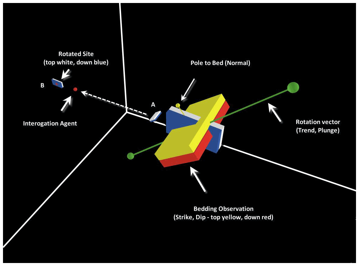
Figure 3 Structural agent demonstrating a quaternion 90^∘ clockwise rotation during linear estimation (SLERP) between two points. Starting point A (local), with equivalent orientation to the larger observation (yellow and red cuboid) and final rotated point B (distal). Rotation maintains smooth topology for top direction. See Appendix B for details.

Figure 4 Spatial agent-based triangular meshing created from the Mesh program. See Appendix B for details.

2.2 Agent communication

There are a wide range of functions, behaviours, and states that can be encoded into the agent set. These are collectively driving what will be a successful application solution. Facilitating the efficient outcome of an agent model are agent communications. Inter-agent communication is handled through agent property updating (Fig. 5). Each agent is responsible for knowing what is going on to the extent that it has been programmed to – for example, a proximity property may be updated that indicates the nearest free agent neighbour, which is an agent that does not yet belong to a swarm. Depending on what behaviour has been programmed into the code, if an agent reaches a certain proximity threshold, an event might be triggered, such as the creation of an association link with a more proximal agent.

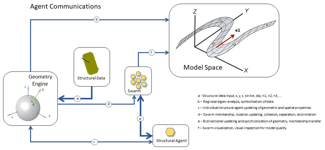
Figure 5 General summary of structural agent communication using the example from GeoSwarm; for details, see comments and codes in the open-source programs listed in Appendix B. The thickness of the blue lines indicates the relative degree of inter-agent communication. The geometry engine is composed of all agent functions for determining eigen-directions, proximity, rotation, location, and spatial estimation. The grey fold surface in model space represents a possible fold realization that emerges from swarming structural agents, given sparse input data (yellow markers). The red arrow indicates the principal eigenvector direction, which is also the fold hinge or regional plunge; this can be used as a rotation axis for updating the structural agent geometry.

An agent can be made to act like an interrogator of space, whereby a continuous sampling may occur, in a given direction rather than through a predefined set of indexed grid cells, such as in a convolution filter. Core to the behaviour of agents is the communication of derived weighting parameters for various properties, most importantly, for structural orientation during interpolation. It is in this way that an agent can define a local neighbourhood as a local swarm, not just by proximity but also with geometric properties such as orientation. An agent might be very close to its neighbour but may not be selected to be in the swarm because it is oriented at an overly high angle; thus, this promotes the collaboration of agents that are near coplanar. Agent interpolation is not actually replacing more classical schemes. SABMs are more of a framework in which interpolation and other spatial operators can be called from as needed. Interpolation schemes from simple to complex could be employed, such as nearest-neighbour, inverse-distance-weighted (IDW), or quaternion-based spherical linear rotation interpolation (SLERP) (De Paor, 1995, 1996; Shoemake, 1985; Hamilton, 1844). Several schemes could be employed depending on local or global data configurations, property conditions, and knowledge constraints. For the demo examples, the extensive use of SLERP methods ensures that the rotations of geologic orientation data are smooth and more realistic with respect to expected structural deformation processes. In the presented examples, there are currently no rheological controls, but these physical parameters could be programmed into the agent rule set. Agents can be programmed to react to physical laws, for example, the barycentre of a three-tuple mesh can be dynamically recalculated when neighbour masses, other material, and mechanical properties are changed. The location and states of all agents are available and are stored at the agent level, passed to a communications centre, or just stored as a global variable, if needed. Agent intercommunication is a significant topic of computational science research (Hall and Virrantaus, 2016; Ménager, 2006) that may have implications for geological modelling – for example, if moving into the field of geological and geophysical integration and joint modelling, agents may have potential in the optimization strategies for inversion of complex-geometry multi-parameter scalar and vector fields (Jessell et al., 2010; Lindsay et al., 2013). The way that agents can communicate specific local to global information states and the way that they can adjust to the combined data and knowledge constraints (Liscano et al., 2000; Friedrich et al., 1999; Gaspari, 1998) may determine the applicability of their use for geological and no doubt other applications as well. For a comprehensive summary of agent and inter-agent communications and agent system controls, the reader is referred to Heppenstall et al. (2012); for a summary of spatial agents with GIS, the reader is referred to Crooks and Heppenstall (2012); and for a practical introduction to spatial agents, the reader is referred to Wilensky and Rand (2015) (see also Appendix A).

2.3 Agent behaviour

The following points outline some interesting qualities of spatial agents:

1. Agents are able to efficiently interrogate irregular and complex model spaces. The model design can result in a wide range of single realizations or solution suites. More traditional approaches are dependent on fixed regular and partitioned structures using standard coordinate systems, with few geological properties.

2. Agents are suitable for modelling natural complex systems. Thus, they are valuable for preserving the contributions from multi-scalar and deep multi-property data, such as fold shape parameters, or geophysical rock properties. Global interpolation techniques, such as implicit interpolation, tend to generalize dense data clusters to a local mean and are optimized for a scale-specific purpose, often producing geologically meaningless results (Fig. 1). This could happen when combining point geometry from structure, categorical geology, and continuous geophysics data. Essential details such as fold topology and hinge regions can be ignored or conflict dramatically with geophysical gradients. Agents may be able to more easily incorporate this kind of local information during estimation and feature propagation.

3. Agents can support the domain expert that requires more interpretive skills, with knowledge-based rules, missions (beliefs), and/or behaviours during data interrogation. Agents could be used in mapping to visualize complex relationships, such as within vector fields, for fabric intersections (bedding–cleavage relationships), vergence relationships on fold trains, disharmonic folds, and poly-deformed stratigraphy with early cryptic faulting. Visualization of these relationships within the event history is critical for more accurate geological interpretation.

4. Agents complement rather than replace existing algorithms and approaches. For example, spatial estimation can still be applied (e.g. implicit; inverse distance weighted – IDW; kriging; discrete smooth interpolation – DSI; support vector machine – SVM) at variable scales as required. Thus, they could potentially provide a framework for calling a variety of interpolators and constructors, depending on data density, problem domain, and feature complexity.

5. Agent interaction and communication may produce group swarm behaviour. This emergence could potentially express more complex features or trigger other spatial topological changes, such as new faults or unconformities. Agents may also spawn, through their state condition, new geologic events – for example, inserting a new deformation event when a metamorphic fabric is observed in a boulder of apparently undeformed conglomerate, or when a high-curvature region is detected by inserting a fold hinge or fault control point.

6. Agent-based approaches may benefit from denser and faster CPU/GPU architecture and parallelization schemes. This could be the case, as the simple rules driving agent interaction and communication act more independently, rather than having to invert large global matrices common in implicit approaches. This is yet to be tested, as it is perhaps hard to partition ongoing spawning processes from independent agents, but could result in dramatic efficiency gains when combining multi-scalar properties from geophysics and geology within 3D structural fields (Burns, 1988; Hillier et al., 2013).

3 Agents examples

To demonstrate the general principals of agent behaviour for geologic surface development, a number of simple applications were developed, using mostly synthetic data, along with one rescaled data set from an Archean greenstone belt, Caopatina, Québec (de Kemp, 2000), in a model space with (X, Y, Z) dimensions of (100, 100, 100) and a model centre at (X, Y, Z) of (0, 0, 0). The NetLogo codes presented are freely available for download (see https://github.com/Loop3D/GeoSwarm.git, last access: 1 October 2021, or https://doi.org/10.5281/zenodo.4634021, de Kemp, 2021).

In the following example scenarios, spatial agents may represent control data, interrogators, or estimated solutions. They could also morph from one type to another. For example, a data agent could extend itself by expanding incrementally along the dip plane directions into estimation points. They may have properties for tracking local swarm or global states, continuously checking for proximity to neighbours, their status as interrogators, or observation sets and their geometric properties, such as strike, dip, and polarity (top direction). Agents may have pointers and links to specific topological neighbours, as in the case of adjacent triangles, but importantly, there is no ordered centralized control list or matrix that holds all of the agents and their relationships. Each type of agent is created and encoded with properties that may change, such as the local anisotropy derived from the eigen-analysis of local supported data. The structural agents are spatial agents, represented herein as tablets or hexagonal glyphs and rotated as quaternions (Fig. 6).

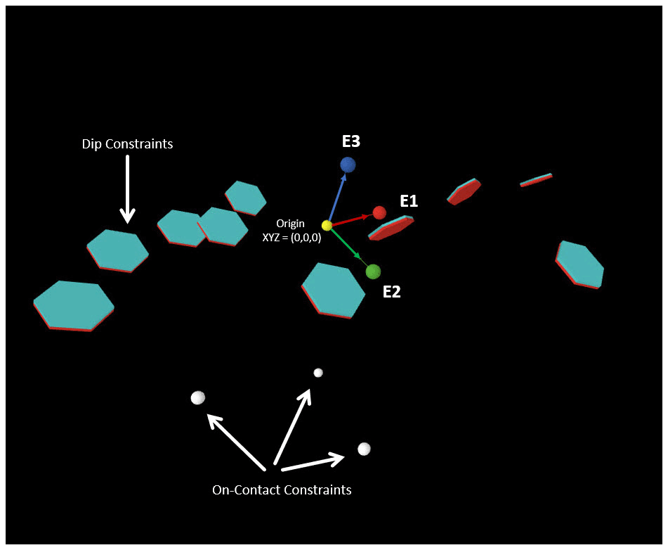
Figure 6 Input data constraints. On-contact (white spheres) and dip (where blue thin hexagonal prisms denote upright, and red thin hexagonal prisms denote the down direction) constraints representing simple 3D geological data constraints. The arrows at the origin indicate the calculated orthogonal unit eigenvector directions for the structural data. Depending on the scenario, the structural agents will do a SLERP interpolation (De Paor, 1995, 1996; Shoemake, 1985; Hamilton, 1844) using a rotation vector from the major global eigenvector axis to simulate the behaviour of bedding rotation due to near-coaxial folding (Woodcock, 1977). For the specific calculations used in each program, see comments in the source code at GitHub open-source website at https://github.com/Loop3D/GeoSwarm (last access: 1 October 2021) (https://doi.org/10.5281/zenodo.4634021, de Kemp, 2021); the reader is referred to Davis and Titus (2017, and the Appendix therein) and Adamuszek et al. (2011) for a thorough review of structural data computations. A summary of the quaternion rotation math is given in Appendix C.

3.1 Scenarios

Each of the following programs runs inside NetLogo 3D, an agent simulation software which is freely available from the Northwestern University NetLogo download site: http://ccl.northwestern.edu/netlogo/ (last access: 29 September 2021). The reader should try the default parameters set when each program is called from NetLogo 3D and then adjust some of the simpler parameters that control global orientation such as strike and dip. The descriptions below give the name of the program, its intended behaviour, and the main purpose of the demonstration code. Note that not all codes have been thoroughly tested or gone through performance optimization. It is best to slowly increase the number of agent data points for each scenario and experiment with the control parameters for the best results.

3.2  Trace

Trace demonstrates the modelling of fabric observations (Fig. 2). The search agent (red sphere) travels through the model space randomly until it senses a proximal dip observation. It will then adjust its trajectory towards a down-dip vector for this observation and spawn other simulated dip points that are nearest-neighbour (NN) or inverse-distance-weighted (IDW) interpolations from the data. A stream of points is recorded as the search agent moves through the model space. This point stream will form De Casteljau–Bézier (Farin, 1997) curves that are either killed or preserved based on simple user-specified shape parameters, such as curve length. Other criteria were not implemented; however, this could be done using local or regional geometry properties, such as degree of curvature, or mean direction angle. Trace demonstrates streamline visualization using down-dip trajectories. It is similar to the 3D structural field interpolation (SFI) from Hillier et al. (2013). The main distinction here is the sampling is random with the potential for multiple search agents acting simultaneously.

3.3  Poly

Poly demonstrates simple polyhedral graphics control which is needed for vector-based boundary representations used in many geological modelling environments. Construction agents can perform simple local tasks, such as making a single polyhedron, but also regional tasks, by joining these up until stop criteria are reached. Modelling of simple closed and connected polyhedra is achieved by joining simple triangles or large loops with many vertices. Each closed polyhedron once formed will connect one link to its adjacent polyhedron, forming a simple object chain. Modelling and visualization of the network are controlled by user-defined edge size, search radius, repulsion, and tension of the edges.

3.4  Rotate

Rotate demonstrates SLERP rotations, which would be required for estimation in complex geological domains, with folding and sparse-data representation (Fig. 3). It is also a testing environment for interpolating planar constraint data with linear rotation axis. The main control dip agent is located at the origin in the centre of the model space and a user-defined target dip agent is set up. A linear quaternion rotation of the control dip is incrementally rotated along a single or circular radial to the target dip. Users can rotate all dips continuously and dynamically. The agents are always updating to the new target. The rotation axis is defined by the user which could be in all possible in-plane or out-of-plane cross-dip orientations. This is a required method for the estimation of local and regional dips and structural vector fields.

3.5  Mesh

Mesh demonstrates the development of topological surfaces that, at a minimum, are defined by a triangulated mesh that has direction and polarity sensitivity (Fig. 4), and also shows that a mesh can be produced from agents without a grid – that is, without having to sample a scalar field value in a partitioned grid (i.e. with marching cube). In addition, it demonstrates that agent-based meshes could be grown locally while conforming to constraint data. Each triangle has a normal that is maintained from the barycentre of the triangle. Triangle vertices have a mass that can be changed by the user to influence the location of the barycentre. A seed triangle senses the nearest-neighbour triangle vertex and attracts it (back to itself). The incoming triangle is rotated to be conformable to the evolving surface patch and connected, keeping the normal pointing in the same way, thereby maintaining simple surface topology. In this way, distributed primitive shapes could act as spatial data interrogators, before being transformed into mesh constructors. Simple topology metrics (edge : vertices : triangle ratios) are reported and plotted on the GUI graph. Once the mesh is complete, if the on-contact constraints are active, the mesh will migrate with its regional barycentre to the nearest on-surface control point, turn it blue from white, and then go on to do the same for the next control point. This functionality is a precursor requirement for adaptive meshes that could potentially be shaped by various spatial and property data, data quality, and data densities. In this instance, a surface mesh is grown through the use of simple geological rules. For example, a surface can not intersect itself, it needs to be continuous with consistent surface polarity, and it also needs to avoid large tear faults. These surfaces may move toward on-contact data constraints to extend the local observations. The ratios of triangles to shared edges and shared vertices can be used to check topology and can be used as a stopping criteria, to reward or penalize during the meshing process.

3.5.1 Swarm dips: simple plane

The program Swarm dips in simple plane mode demonstrates the convergence of a non-meshed swarm toward a common plane. It is useful to demonstrate proximity, vision distance effects, angle of sight, and separation. Randomly initialized interrogation agents, represented as smaller hexagons and herein referred to as “Dip Sims”, are dynamic sensing agents and are used to estimate or simulate local structural vector fields. These Dip Sims slowly behave as a swarm, moving in the plane specified by the controller, respecting vision-proximity and view-angle rules. When the separation and vision distance are low, the sims will converge and produce red balls, alerting the user that a proximity threshold has been crossed. The red balls disappear once the sims move apart, and the inter-sim distance is greater than the specified separation. This mode uses a single main dip controlling agent, represented by a large origin (0, 0, 0) centred, two-sided (yellow (up)–green (down)) hexagon (see Fig. 7). The displayed data for on-contact and stationary dip data have no influence. Only the main controller, large green–yellow hexagon symbol that is stationary at the model centre with the orientation (strike, dip, polarity) defined by the user, influences the swarm. The controlling parameters are adjusted dynamically during the simulation run, initiated by first pushing the “setup” and then the “simulate” buttons. Dip Sims sense other Dip Sims within the vision distance and the view angle (ϕ), and they are kept from one another by a user-defined separation distance (yellow circle). The user changes the configuration during a simulation with the sliders on the NetLogo interface to control strike and dip properties of the main dip which, in turn, controls the plane upon which agents are moving. The data in all of the swarm examples are generated artificially by randomly positioned sites on the plane of the main controller. The orientation of each dip data point is set by random rotation perpendicular to the E1 (eigen) axis, to achieve a user-specified variability (0 denotes no dip variance, and 1 denotes maximum dip variance). The idea is that each agent can see other agents within a locally controlled environment such as a given vision distance and angle of sight, and these other agents start to coalesce and form a swarm, which could potentially have some task to complete – for example, extending a geologic feature of interest or extending a depositional horizon.

Figure 7 Components of the spatial agent-based model (SABM).

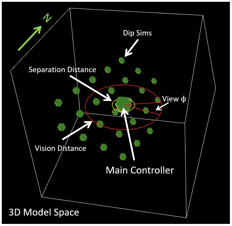
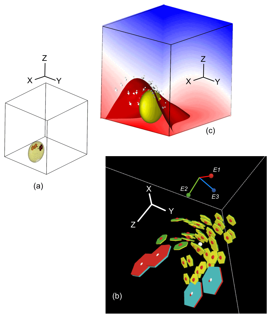
Figure 8 Surface model (closed yellow ellipsoid) utilizing implicit calculations with SURFE (Hillier et al., 2014) obtained by using only four on-contact dip data points (a) and then using the GeoSwarm program to extend a fold plunge, with 50 off-contact spatial structural agents depicted from the bottom (looking up) in panel (b). The red surface in panel (c) is a more spatially continuous antiformal structure, obtained using the structural agent approach, than the structure obtained using implicit codes alone. Note that eigenvector E1 (red stick and ball) is pointing down the plunge of the fold, which is the strongest continuity direction.

3.5.2 Swarm dips: moving plane with dips

Swarm dips in moving plane with dips mode demonstrates smooth linear interpolation using SLERP (spherical linear rotation interpolation) with quaternions, and parameterizes the rotation with linear segmentation of straight-line distance to controlling dip data. As the Dip Sims come close to static dip data control points, they will adjust their local orientation to match the orientation properties of the data but do not move spatially towards these off-contact orientation observations (Fig. 7).

The influence of the orientation data on the estimation of orientation properties at the Dip Sim is weighted in an inverse distance manner. There is no migration to on-contact data, and only the off-contact dip data points have influence. Outside the vision distance, the main regional controller determines the agent orientation.

3.5.3 Swarm dips: migrate to on-contact data

Swarm dips in migrate to on-contact mode demonstrates that sims can sense and migrate to on-contact feature control points while detecting the structural influence from adjacent data. Dip Sims move toward the nearest on-contact data point while rotating into parallelism with the closest dip observation. At a given tolerance to the on-contact data points, the Dip Sim freezes in an orientation that is close to the neighbourhood dip field. When all on-contact data points have a Dip Sim, the rest of the Dip Sims will behave as a swarm: controlled by the main controller and moving in the plane specified by the controller and vision-proximity rules.

3.6  GeoSwarm

This example incorporates all of the above swarm methods using four separate structural observation files or a random set. The four test sets are taken from actual field data gathered from the Caopatina region, Québec, Canada, from steeply dipping and folded series (Fig. 8) of turbiditic sediments from an Archean greenstone belt (de Kemp, 2000). Scaling settings can stretch the extents of the data for testing local versus regional influences on swarm cohesion. Several distance-sensitive parameters determine how agents are weighted for local surface cohesion versus data migration. A file I/O (input/output) interface is used to test various data configurations representative of common but simple geologic fold scenarios. It could be adapted for custom data configurations and will be used in the future for parameter selection training and testing with a range of real data sets.

4 Discussion and conclusions

This study focuses on the rudimentary requirements for geological modelling using spatial agents, primarily their ability to interrogate, communicate, and represent solutions to simple sparse geometric or structural constraint data configurations. No doubt future research needs to go much further to establish how to build full geological models, optimizing the arsenal of existing geospatial tools within an agent framework. Initial indications are promising for the use of agents to develop meshing tools, topologically sensitive surface construction of objects, and for respecting simple geological data constraints such as on-contact and dip observations.

The use of eigenvectors to summarize local anisotropic conditions derived from dip populations was helpful in supporting the propagation of agents, weighting of the spatial continuity direction in a more intuitive manner for structural geological interpretation, and selection of rotation axis for quaternion interpolations. These techniques, more commonly used in the graphics industry (Liu et al., 2013), would be generally beneficial going forward in 3D structural geological modelling and also potentially for more elaborate spatial agent approaches when solving for multi-property anisotropies such as those that occur in natural geophysical and geological property distributions (De Paor, 1995, 1996). Sparse-data configurations with more structural variability (see Fig. 8) supported with an agent approach will better reflect and extend local structural anisotropy when modelling using other methods, such as with implicit estimators.

With the abundance of machine learning tools currently available, it would be potentially useful to investigate how to optimize structural agents for particular geological use cases – for example, using self-organizing maps and generalizations for up-scaling structural data sets based on sampling from Kent distributions (Carmichael and Aillères, 2016) for regional 3D modelling or with the application of graph neural networks for more complex geological modelling with sparse data (Hillier et al., 2020) as well as other emerging deep learning approaches (Guo et al., 2021; Zhang et al., 2019).

Natural examples of agent behaviour, such as swarm behaviour, have emerged over millennia through the embedding of simple rules into organisms that have evolved for the optimization of their group survival. This paradigm, although perhaps not obvious for geological applications, could take a similar path and could be an opportunity to leverage geological knowledge through the embedding of specific behaviours for given geological processes that are controlled through simple geological rule sets – for example, by programming agents to maintain a range of thickness between stratigraphic layers as they are propagated regionally. Importantly, geological agents would need to operate in a geologically reasonable framework, respecting the local or regional geological topology network (Thiele et al., 2016). They would need to be able to create solutions from a suite of possible geological topologies with more complex feature sets – for example, from combinations of geologic contacts and overprinting, such as from horizons, faults, ore bodies, intrusions, alteration, and metamorphic fabric relations.

From this study, it is clear that spatial agents can be used to develop simple meshed surfaces, fabric traces, and to visualize anisotropies and structurally sensitive swarm surfaces. Structural agent interrogators exploring a model space can update local or group behaviour to conform to on-contact dip constraints, or to a constraining vector field within a volume.

Agent-based tools as applied to geological applications are still in their infancy but can be used to interpolate or extrapolate from data to produce fabric trajectories, gradients, vector fields, and continuous or discontinuous polyhedral meshed surfaces. The amplification of local anisotropies is particularly useful with sparse-data and increased structural complexity scenarios. These characteristics can provide support for simulated input using existing methods for spatial estimation, such as implicit approaches.

Finally, more in-depth investigation into the use and optimization of spatial agents needs to be undertaken to demonstrate the range of benefits for complex geological modelling in a variety of data configurations that could represent typical geological scenarios.

Appendix A: Agent resources

An excellent starting point to become familiar with agent-based applications and approaches is Paul Torrens' website (http://geosimulation.org/, last access: 1 October 2021) from the Tandon School of Engineering and the Center for Urban Science and Progress at New York University.

The agent-based codes used in this paper are written in NetLogo 3D, a spatial agent-based modelling language and development environment that is supported by the Center for Connected Learning and Computer-Based Modeling in Evanston, Illinois, USA. The NetLogo project is affiliated with Northwestern University Centre on Complex Systems (NICO; https://www.nico.northwestern.edu/, last access: 1 October 2021). To download and run the NetLogo codes, and for tutorials and documentation on the NetLogo language, see http://ccl.northwestern.edu/netlogo/ (last access: 1 October 2021). The code must be minimally compatible with the NetLogo 3D version, as listed in the programs below (Table B1). Current and early 3D versions of the program are all available on the main NetLogo home page.

Codes presented in this paper are freely downloadable from the GitHub open-source website at https://github.com/Loop3D/GeoSwarm.git (last access: 1 October 2021) (https://doi.org/10.5281/zenodo.4634021, de Kemp, 2021), with the accompanying power point, PDF, and animations presented at the annual meeting of the International Association of Mathematical Geoscientists at Penn State University, USA, August 2019.

Appendix B

B1 List of NetLogo 3D programs

Table B1 Summary of demonstration programs.

B2 Example pseudocode

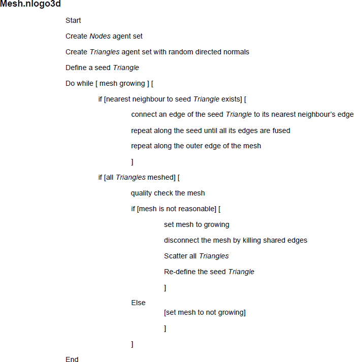
As seen above, once all of the meshing is complete, there is a quality control check to determine if the result is a “reasonable” surface. This could be a simple rule that looks for holes and for surfaces with low connectivity, for example, by calculating a low node count to edge count ratio: a ratio of 1 infers no triangles connected, ∼0.72 infers a single node connected chain, ∼0.62 infers a single edge connected chain, and ∼0.58 infers a hexagonal mesh.

Appendix C: Quaternion calculations

Quaternion codes are used in the Dip_Swarm and Rotate programs and implemented in NetLogo within the Spin() procedure to ensure smooth rotation along a specified axis, such as an eigenvector of a structural observation set and for inverse-distance-weighted (IDW) and spherical linear rotation interpolation (SLERP). For details, see De Paor (1995, 1996), Shoemake (1985), and Hamilton (1844).

C1 Provide a normalized unit vector to the Spin procedure from common structural observation data

In order to provide a normalized unit vector to the Spin procedure from common structural observation data, the user must convert strike and dip (RHR) to a unit normal vector. Here, the input is in degrees, and the normal is perpendicular to the plane.

• “strike” is a scalar angle of in degrees azimuth in the horizontal plane measured clockwise from north (0^∘) that represents the angle between a topographic surface trace of a geological feature, such as a horizon intersecting with topography, and the north direction. Strike in this study uses the right-hand rule (RHR), which is a common structural geological measuring standard for planar field observation data. It assumes that the strike direction vector is pointing such that the geological surface dips to the right of the observer as they face the strike direction. (Note that east is equal to 90^∘, south is equal to 180^∘, and west is equal to 270^∘.)

• $$\begin{array}{}\text{(C1)}& \mathit{\text{strike}}\in \left\{\mathrm{0},\mathrm{360}\right\}\end{array}$$

• “dip” is a scalar angle in degrees indicating the maximum slope from the horizontal taken in the direction of the dipping surface. The dip direction is always 90^∘ to the strike direction. The dip angle (dip) is the maximum vertical angle from the horizontal to the geological surface.

• $$\begin{array}{}\text{(C2)}& \mathit{\text{dip}}\in \left\{\mathrm{0},\mathrm{90}\right\}\end{array}$$
• $$\begin{array}{}\text{(C3)}& \mathit{\text{polarity}}\in \left\{-\mathrm{1},\mathrm{0},\mathrm{1}\right\}\end{array}$$

• “polarity” is a signed unit integer indicating if a geological surface is upside down – that is, overturned with respect to its original depositional configuration: a value of −1 denotes overturned, a value of 0 denotes unknown, and a value of 1 denotes upright. This value is used to give topological information in modelling.

• $$\begin{array}{}\text{(C4)}& \mathit{\text{strdip2norm}}\left(\mathit{\text{strike, dip, polarity}}\right)\end{array}$$

• This function will return a three-element unit normal vector.

• The down-dip vector is calculated as follows:

  $$\begin{array}{c}{\displaystyle }ddx=\cos (-\mathrm{1}\times \mathrm{strike})\times \cos (-\mathrm{1}\times \mathrm{dip})\\ {\displaystyle }ddy=\sin (-\mathrm{1}\times \mathrm{strike})\times \cos (-\mathrm{1}\times \mathrm{dip})\\ {\displaystyle }ddz=\sin (-\mathrm{1}\times \mathrm{dip}).\end{array}$$

  The strike vector is calculated as follows:

  $$\begin{array}{c}{\displaystyle }sx=-\mathrm{1}\times \mathrm{ddy}\\ {\displaystyle }sy=ddx\\ {\displaystyle }sz=\mathrm{0}.\end{array}$$

  (Note that the strike vector is always in the horizontal plane.)

  The user can then cross the down-dip vector with the strike vector (V_dd X V_s) to get the normal (N) or pole to bedding:

  $$\begin{array}{c}{\displaystyle }NNx=(ddy\times sz)-(ddz\times sy)\\ {\displaystyle }NNy=(ddz\times sx)-(ddx\times sz)\\ {\displaystyle }NNz=(ddx\times sy)-(ddy\times sx).\end{array}$$

  The following equation normalizes the normal for unit length L:

  $$L=\sqrt{NN{x}^{\mathrm{2}}+NN{y}^{\mathrm{2}}+NN{z}^{\mathrm{2}}}.$$

  The user can then adjust for polarity:

  $$\begin{array}{c}{\displaystyle }Nx=(\mathrm{polarity}\times NNx)/L\\ {\displaystyle }Ny=(\mathrm{polarity}\times NNy)/L\\ {\displaystyle }Nz=(\mathrm{polarity}\times NNz)/L.\end{array}$$

  The following equations are able to convert a trend and plunge to a normalized unit vector: a common fabric element for various linear structural features such as fold hinge lines joining maximum curvatures along the plunge of a fold, or stretching features located along E3. This is then used to get a vector from an agent heading and pitch state.

• TrendPlunge2Vec (trend, plunge)

• This function returns a three-element unit normal vector.

  $$\begin{array}{c}{\displaystyle }VVx=\sin \left(\mathrm{trend}\right)\times \cos \left(\mathrm{plunge}\right)\\ {\displaystyle }VVy=\cos \left(\mathrm{trend}\right)\times \cos \left(\mathrm{plunge}\right)\\ {\displaystyle }VVz=\sin \left(\mathrm{plunge}\right)\end{array}$$

  The unit vectors are normalized as follows:

  $$\begin{array}{c}{\displaystyle }M=\sqrt{VV{x}^{\mathrm{2}}+VV{y}^{\mathrm{2}}+VV{z}^{\mathrm{2}}}\\ {\displaystyle }Vx=VVx/M\\ {\displaystyle }Vy=VVy/M\\ {\displaystyle }Vz=VVz/M.\end{array}$$

C2 Input the rotation increments (A), the rotation vector (Q), and the normal of the structural observation (P) into the Spin procedure to rotate the structural elements with quaternion calculations

C2.1 Spin (A, V, P)

Input arguments to Spin are A, V, and P.

• A is the spherical angle of rotation in degrees (not Euler angles): $A\in \left\{-\mathrm{\infty },\mathrm{\infty }\right\}$.

• V is the unit vector 3D axis of rotation (Vx, Vy, Vz,) and can be any of the eigenvectors (e.g. a down-dip vector or a strike vector).

• P is the normal unit vector (n_x, n_y, n_z) (e.g. poles to beds or a fold hinge).

• A new matrix S is calculated with a full orientation description, including the normal to bedding or new rotated linear element, the strike and dip components, overturned (polarity), and four quaternion elements (qw, qx, qy, qz). This is then transformed from a single vector to quaternion with rotation A about an axis Q. This procedure can be used to convert normal to strike and dip RHR by inputting A=0 rotation and V=P each cast as three-element normal vectors. This returns a RHR_Orientation array using a right-hand rule planar orientation for strike, dip, n₁, n₂, and n₃, and overturned.

  $$\begin{array}{c}{\displaystyle }\mathit{Q}=(s,\mathit{V})\text{scalar, vector}\\ {\displaystyle }qx=\left(\sin \right(A/\mathrm{2})\times Vx\\ {\displaystyle }qy=\left(\sin \right(A/\mathrm{2})\times Vy\\ {\displaystyle }qz=\left(\sin \right(A/\mathrm{2})\times Vz\\ {\displaystyle }qw=\left(\cos \right(A/\mathrm{2}\left)\right)\\ {\displaystyle }\mathit{Q}=(qw,qx,qy,qz)\end{array}$$

C3 Create the rotation matrix

To create the rotation matrix, the user can utilize quaternion identities to derive the rotation matrix:

$$\begin{array}{c}{\displaystyle }q\mathrm{2}w=\mathrm{1}-q{x}^{\mathrm{2}}-q{y}^{\mathrm{2}}-q{z}^{\mathrm{2}}\\ {\displaystyle }q\mathrm{2}x=q{x}^{\mathrm{2}}\\ {\displaystyle }q\mathrm{2}y=q{y}^{\mathrm{2}}\\ {\displaystyle }q\mathrm{2}z=q{z}^{\mathrm{2}}.\end{array}$$

One can then compose R, the rotation matrix as follows:

$$\begin{array}{c}{\displaystyle }\mathbf{R}=\begin{array}{lll}q\mathrm{2}w+q\mathrm{2}x-q\mathrm{2}y-q\mathrm{2}z& \mathrm{2}qxqy-\mathrm{2}qzqw& \mathrm{2}qzqx+\mathrm{2}qyqw\\ \mathrm{2}qxqy+\mathrm{2}qzqw& q\mathrm{2}wq\mathrm{2}x+q\mathrm{2}y-q\mathrm{2}z& \mathrm{2}qyqz-\mathrm{2}qwqx\\ \mathrm{2}qzqx-\mathrm{2}qyqw& \mathrm{2}qyqz+\mathrm{2}qwqx& q\mathrm{2}wq\mathrm{2}x-q\mathrm{2}y+q\mathrm{2}z\end{array}\\ {\displaystyle }\mathbf{R}=\begin{array}{lll}{R}_{xx}& R_{xy}& R_{xz}\\ R_{yx}& R_{yy}& R_{yz}\\ R_{zx}& R_{zy}& R_{zz}.\end{array}\end{array}$$

C4 Final rotation

Following this, the user can matrix multiply the rotation matrix by the input observation normal P:

$$\mathit{S}=\mathit{P}X\mathbf{R}.$$

C5 SLERP Interpolation

The user can then interpolate by calling the spherical linear rotation interpolator (SLERP) for any interpolation on parameter t, a normalized distance between data and the spatial starting point of an agent (A) as it is rotated towards the structural constraint (B). Details of SLERP can be located in De Paor (1995, 1996). Note that with the inverse-distance-weighted (IDW) form of SLERP, a set of structures can influence the agent depending on the agent's ability to sense the data, for example, the structural search agent needs to be within the vision distance.

For the IDW form of SLERP, the user can calculate the data weights based on the inverse distance and can adjust exponent ^p, if needed, for stronger local influence:

$$W_i={\displaystyle \frac{\mathrm{1}}{D_i^p{\sum }_{j=\mathrm{1}}^n\left(\frac{\mathrm{1}}{D_j^p}\right)}}.$$

The user can then calculate G, the estimated orientation at x, by adjusting the contributing quaternion components of the data with the distance weights:

$$\mathbf{G}\left(x\right)=\sum _{i=\mathrm{1}}^n\left(W_i\times Q_i\right).$$

To use the simpler linear form with A and B orientations,

$$\mathrm{SLERP}\left(x\right)=\left(\mathrm{1}-t\right){\mathit{Q}}_{\mathrm{A}}+t{\mathit{Q}}_{\mathrm{B}}(t=|\mathrm{dist}\left|\right).$$