Effect of horizontal resolution on the simulation of tropical cyclones in the Chinese Academy of Sciences FGOALS-f3 climate system model

The effects of horizontal resolution on the simulation of tropical cyclones were studied using the Chinese Academy of Sciences Flexible Global Ocean–Atmosphere–Land System Finite-Volume version 3 (FGOALS-f3) climate system model from the High-Resolution Model Intercomparison Project (HighResMIP) for the Coupled Model Intercomparison Project phase 6 (CMIP6). Both the low-resolution (about 100 km resolution) FGOALS-f3 model (FGOALS-f3-L) and the high-resolution (about 25 km resolution) FGOALS-f3 (FGOALS-f3-H) models were used to achieve the standard Tier 1 experiment required by HighResMIP. FGOALS-f3-L and FGOALS-f3-H have the same model parameterizations with the exactly the same parameters. The only differences between the two models are the horizontal resolution and the time step. The performance of FGOALS-f3-H and FGOALS-f3-L in simulating tropical cyclones was evaluated using observations. FGOALS-f3-H (25 km resolution) simulated more realistic distributions of the formation, movement and intensity of the climatology of tropical cyclones than FGOALS-f3-L at 100 km resolution. Although the number of tropical cyclones increased by about 50 % at the higher resolution and better matched the observed values in the peak month, both FGOALS-f3-L and FGOALS-f3-H appear to replicate the timing of the seasonal cycle of tropical cyclones. The simulated average and interannual variabilities of the number of tropical cyclones and the accumulated cyclone energy were both significantly improved from FGOALS-f3-L to FGOALS-f3-H over most of the ocean basins. The characteristics of tropical cyclones (e.g., the average lifetime, the wind–pressure relationship and the horizontal structure) were more realistic in the simulation using the high-resolution model. The possible physical linkage between the performance of the tropical cyclone simulation and the horizontal resolution were revealed by further analyses. The improvement in the response between the El Niño–Southern Oscillation and the number of tropical cyclones and the accumulated cyclone energy in FGOALS-f3 contributed to the realistic simulation of tropical cyclones. The genesis potential index and the vorticity, relative humidity, maximum potential intensity and the wind shear terms were used to diagnose the effects of resolution. We discuss the current insufficiencies and future directions of improvement for the simulation of tropical cyclones and the potential applications of the FGOALS-f3-H model in the subseasonal to seasonal prediction of tropical cyclones.

1 Introduction

Tropical cyclones are extreme weather phenomena characterized by intense wind speeds and heavy rainfall. Although tropical cyclones alleviate coastal droughts, they can also cause severe economic losses and significant human casualties (Mendelsohn et al., 2012; Benfield, 2018). Against the current background of global climate change, the effective simulation, prediction and projection of global tropical cyclone activity are challenging but essential for disaster prevention and mitigation (Emanuel, 2017).

The simulation of tropical cyclones in global climate models (GCMs) is challenging in terms of both resolution and physical processes. Tropical cyclone-like structures appeared in early GCMs and Manabe et al. (1970), Bengtsson et al. (1982), Krishnamurti and Oosterhof (1989), Manabe and Broccoli (1990), Wu and Lau (1992) and Haarsma et al. (1993) were pioneers in using objective feature-tracking approaches to study simulated tropical cyclones. However, the low-resolution, incomplete parameterization of the physical processes in these early GCMs meant that their performance in simulating tropical cyclones was limited. For this reason, statistical methods were used to study the climatology of tropical cyclones. Camargo (2013) found that the simulation of the frequency of tropical cyclones in the Coupled Model Intercomparison Project phase 5 (CMIP5) was much lower than in the observations. This was mainly due to the cold biases in the sea surface temperature, which amplified the uncertainty in future projections. Emanuel (2013) designed a downscaling method to reduce the uncertainty in projections of tropical cyclone activity.

The horizontal and vertical resolutions of climate system models have increased over the last few decades, in line with the complex parameterization of the physical processes. As a result, more refined details (e.g., tropical cyclones and tropical waves) can now be resolved. Regional climate system models with smaller spatial scales and lower computing costs can now be used to simulate tropical cyclones. Knutson et al. (2007) used a high-resolution regional model to simulate tropical cyclone activity in the northern Atlantic Ocean. The structure and interannual variability of the simulated tropical cyclones have a high fidelity with the observations. There has also been a significant increase in the resolution of GCMs (Kim et al., 2014; Small et al., 2014; Li and Sriver, 2018; Scoccimarro et al., 2017; Balaguru et al., 2020). Oouchi et al. (2006) used a 20 km mesh global atmospheric model to simulate tropical cyclone activity in a warming climate and found that the high-resolution GCM could not only describe the details of typhoons very well but also captured the variability of tropical cyclones. Zhao et al. (2009), Knutson et al. (2007), Murakami et al. (2012), Manganello et al. (2012), Strachan et al. (2013) and Zarzycki and Jablonowski (2015) showed that high-resolution GCMs can simulate many of the characteristics of tropical cyclones. The uncertainty in simulating tropical cyclones has been reduced with an increase in resolution, the reasonable parameterization of the physical processes and improvements in the downscaling method (Walsh et al., 2015, 2016; Camargo and Wing, 2016).

The increase in the horizontal resolution of GCMs has led to significant changes in the simulation of the variability of tropical cyclones. The changes can be broadly attributed to two reasons: (1) changes in the large-scale factors; and (2) the development of physical process parameterization and air–sea coupling related to the simulation of tropical cyclones. High-resolution GCMs need to not only give a better description of the structure of tropical cyclones but should also simulate well the relationship between tropical cyclones and large-scale variabilities – for example, the El Niño–Southern Oscillation (ENSO), the Madden–Julian oscillation, wind shear and vorticity, and humidity – which is crucial in reducing the uncertainties in the simulation and prediction of tropical cyclones (Manganello et al., 2012, 2016; Zhang et al., 2016; Delworth et al., 2020). Previous studies have shown that there are significant changes in the ENSO as the horizontal resolution of GCMs increases (Philander et al., 1992; Knutson et al., 1997; Schneider et al., 2003; Masson et al., 2012; Larson and Kirtman, 2013; Meehl et al., 2020) and the simulation results are mostly positive. However, these improvements in predicting the ENSO with an increase in horizontal resolution did not lead to improvements in the relationship between the ENSO and tropical cyclones (Matsuura et al., 1999; Bell et al., 2014; Krishnamurthy et al., 2016). There is also a relationship between the Madden–Julian oscillation and tropical cyclones (Liebmann et al., 1994; Hall et al., 2001; Camargo et al., 2008, 2009; Zhang, 2013; Klotzbach, 2014).

As the horizontal resolution in the models increases, some key parameters in the physical parameterizations are tuned to give a better performance (Bacmeister et al., 2014; Roberts et al., 2020) – for example, Lim et al. (2015) found that an increase in the threshold of minimum entrainment led to increasing tropical cyclone activity and Murakami et al. (2012) found that the constrained convective heating in the convective-scheme-induced intense grid-scale upward motion and promoted large-scale condensation, which favored the development of a more intense tropical cyclone. These artificial tuning methods might introduce more uncertainties in terms of the effects of resolution, giving rise to conclusions that are ambiguous to the tropical cyclone research community. In addition, considering the air–sea coupling process will also affect the simulation performance of tropical cyclone activities, especially with respect to the intensity. Scoccimarro et al. (2017) found that an increased horizontal resolution of the model components was not sufficient to simulate intense and fast-moving tropical cyclone events and that air–sea coupling with a higher coupling frequency helps to improve the performance of simulations of tropical cyclone intensity.

The impacts of horizontal resolution on the simulation of tropical cyclones were studied using the Chinese Academy of Sciences Flexible Global Ocean–Atmosphere–Land System Finite-Volume version 3 (FGOALS-f3) model, which was developed by the State Key Laboratory of Numerical Modeling for Atmospheric Sciences and Geophysical Fluid Dynamics (LASG), Institute of Atmospheric Physics (IAP). The simulated tropical cyclones in FGOALS-f3 were introduced first, then the outputs of FGOALS-f3-L and FGOALS-f3-H were used to reveal the influence of horizontal resolution on these simulations. The latest version of FGOALS-f3 participated in the CMIP6 (Eyring et al., 2016), DECK and MIP endorsements (Zhou et al., 2016; He et al., 2019, 2020; Haarsma et al., 2016). FAMIL2 is the atmospheric component of the FGOALS-f3 climate system model. Li et al. (2019) evaluated the simulation performance of tropical cyclone activity in the latest-generation atmospheric general circulation models from the LASG-IAP (Finite-volume Atmospheric Model version 2; FAMIL2) using a coarse resolution with standard AMIP experiments. Although FAMIL2 is able to reproduce many aspects of the activities of tropical cyclones with a horizontal resolution of 1^∘, there is still some room for improvement in simulating tropical cyclones, such as the weak intensity of tropical cyclones, fewer tropical cyclones in the peak month in the northern Atlantic and eastern Pacific oceans, and inaccurate large-scale factors. Therefore, the the High-Resolution Model Intercomparison Project (HighResMIP) configuration has been applied to both the low- and high-resolution FGOALS-f3. Both model versions retained the exact model physics and parameters and the only differences were the horizontal resolution and model time step, which better meet the rule of HighResMIP: “the experimental set-up and design of the standard-resolution experiments will be exactly the same as for the high-resolution runs”. This study aimed to address the following issues: (1) the impacts of horizontal resolution on the simulation of global tropical cyclones in a climate system model; and (2) the possible physical linkages between the horizontal resolution and the simulated tropical cyclones.

This paper is organized as follows. Section 2 introduces the model, data and methods used in this study. Section 3 shows the performance of simulated tropical cyclones in both FGOALS-f3-L and FGOALS-f3-H. Section 4 introduces the possible reasons for the improvement in the simulation of tropical cyclones with an increased horizontal resolution. Section 5 discusses the impact of physical parameterization and air–sea coupling on the simulated tropical cyclones in GCMs, then discusses the potential value-added effect of large-scale factors related to simulated tropical cyclones when the horizontal resolution is increased from the HighResMIP models. Section 6 summarizes our results.

2 Model, data and methods

2.1 Description of FGOALS-f3

FGOALS-f3 is the latest version of the Chinese Academy of Sciences climate system model and was designed for CMIP6. The FGOALS-f3 model consists of four components: (1) an atmospheric component; (2) an oceanic component; (3) a land surface component; and (4) a sea ice component. The atmospheric component is FAMIL2.2 (Zhou et al., 2015; Bao et al., 2018; Bao and Li, 2020; Li et al., 2019; He et al., 2019), which is the successor to the atmospheric general circulation model of the Spectral Atmosphere Model of LASG (SAMIL) (Wu et al., 1996; Bao et al., 2010, 2013). The oceanic component is the LASG-IAP Climate System Ocean Model version 3 (LICOM3) (Liu et al., 2012). Orthogonal curvilinear coordinates and a tripolar grid are used in LICOM3 and the horizontal resolution can vary flexibly between 1 and $\mathrm{1}/\mathrm{20}$^∘. A new advection scheme has also been updated in LICOM3 (Yu et al., 2018). The land surface component is the Community Land Model version 4.0 (CLM4) (Oleson et al., 2010; Lawrence et al., 2011) with the processes from the dynamic global vegetation model in CLM4.0 used in FGOALS-f3-L/H turned off. The sea ice component is the Los Alamos Sea Ice Model version 4.0 (CICE 4.0; Hunke et al., 2008; Hunke and Lipscomb, 2010). These four components are coupled by the version 7 coupler in the Community Earth System Model (CESM) (Craig et al., 2012). Li et al. (2019) introduced the atmospheric component FAMIL2 in detail and carried out some tuning to achieve stability in long-term coupled integrations (defined as FAMIL2.2).

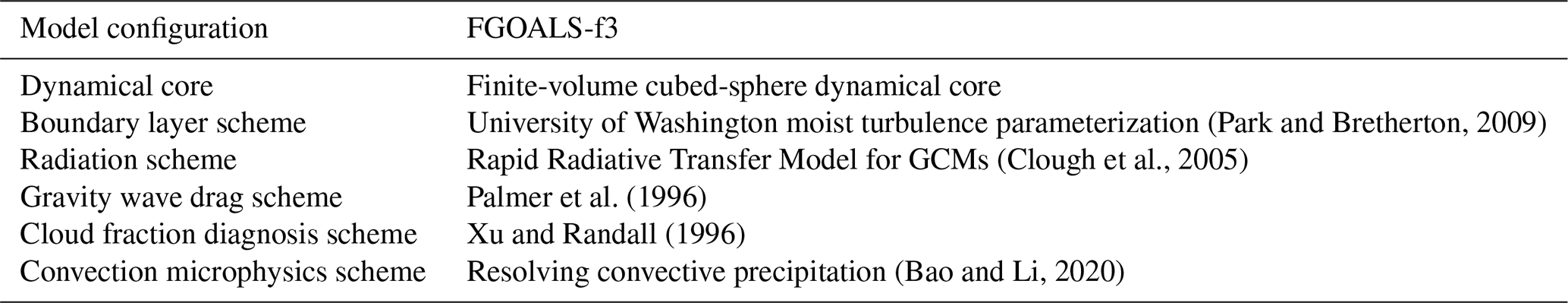
Table 1 shows that the finite-volume cubed-sphere dynamical core (FV3) (Lin, 2004; Putman and Lin, 2007; Voosen, 2017) is used as the dynamical core in FAMIL2.2. The University of Washington moist turbulence parameterization (Park and Bretherton, 2009) is also used in FGOALS-f3. This is a non-local, high-order closure scheme and uses the diagnosed turbulent kinetic energy to determine the eddy diffusivity in turbulence. The resolving convective precipitation (RCP) parameterization (Bao and Li, 2020) is used, which involves calculating the microphysical processes in the cumulus scheme for both deep and shallow convection; six species are considered, similar to the Geophysical Fluid Dynamics Laboratory (GFDL) cloud microphysics scheme (Zhou et al., 2019). The gravity wave drag scheme (Palmer et al., 1986), the cloud fraction diagnosis scheme (Xu and Randall, 1996) and the radiative transmission scheme (Clough et al., 2005) are also considered.

Table 1 Dynamical core and physics parameterization schemes used in FGOALS-f3.

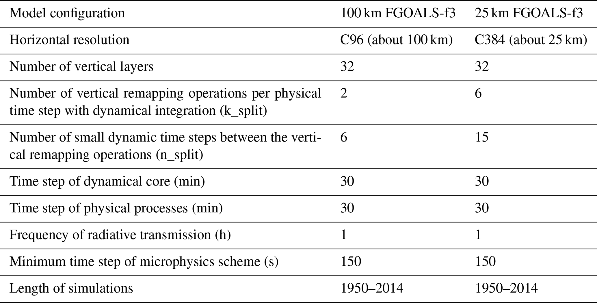
The vertical layers of FGOALS-f3-L and FGOALS-f3-H are both set to 32, whereas the horizontal resolutions of FGOALS-f3-L and FGOALS-f3-H are C96 (about 100 km) and C384 (about 25 km), respectively (Table 2). To maintain the stability of the integration for the dynamical core, the two parameters (k_split and n_split) included in FV3 are different in FGOALS-f3-L and FGOALS-f3-H. k_split is the number of vertical remapping operations per physical time step in the dynamical integration and n_split is the number of small dynamic (acoustic) time steps between the vertical remapping operations, which will affect the stability of the integration when the horizontal resolution of the model is changed. Considering that FGOALS-f3-H requires more frequent vertical remapping, k_split and n_split are set to 6 and 15, respectively (they are 2 and 6, respectively, in FGOALS-f3-L). The time steps of the physical processes are both set to 30 min, but the update frequency of radiative transmission and the minimum time step of the microphysics scheme in both FGOALS-f3-L and FGOALS-f3-H are 1 h and 150 s, respectively. Li et al. (2017) tested the computing performance between FGOALS-f3-L and FGOALS-f3-H using the Tianhe-2 supercomputer and the results indicated a high computing speed-up and low computing costs when the number of parallel processes was increased.

Table 2 Comparison of resolutions, time steps and length of simulations in FGOALS-f3 for HighResMIP Tier 1.

2.2 Datasets

FGOALS-f3 participated in CMIP6 DECK (Eyring et al., 2016), the Global Monsoons Model Intercomparison Project (GMMIP; Zhou et al., 2016; He et al., 2019) and HighResMIP (Haarsma et al., 2016). The datasets from CMOR for the CMIP6 HighResMIP are in a standard format. The experimental design satisfies the requirement for HighResMIP Tier 1. Two resolutions of FGOALS-f3 are used to compare the simulation of tropical cyclone activities at different resolutions. To identify the impact of resolution, there was no tuning of the parameterization of the physical processes between FGOALS-f3-L and FGOALS-f3-H. The time period 1991–2014 is extracted to avoid the uncertainties in the pre-satellite era in the observations.

The International Best Track Archive for Climate Stewardship v03r10 (IBTrACS; Knapp et al., 2010) is used as the observational dataset. IBTrACS is a multisource dataset and includes the RSMC Tokyo, Chinese Meteorological Administration–Shanghai Typhoon Institute (Ying et al., 2014) and the National Hurricane Center data sources. To provide a fair comparison, transformation from the 10 min-averaged maximum sustained wind to the 1 min-averaged maximum sustained wind is needed and the relevant coefficient is set to 0.88 (Manganello et al., 2012; Knapp et al., 2010; Li et al., 2019). The European Centre for Medium-Range Weather Forecasts ERA-Interim reanalysis dataset (Dee et al., 2011) (resolution 0.75^∘), the National Centers for Environmental Prediction Global Forecast System (GFS) reanalysis dataset (resolution 0.25^∘) and the Global Precipitation Measurement (GPM) dataset (resolution 0.25^∘) (Hou et al., 2014) for the time period 1991–2014 are used as the observations to quantitatively evaluate the tropical cyclones simulated in FGOALS-f3.

2.3 Tracking algorithms

An objective feature-tracking approach is used to detect the model-generated tropical cyclones based on the 6 h outputs of FGOALS-f3-L and FGOALS-f3-H. According to the tracking scheme (Table 3), the sea-level pressure, warm core (the temperature anomaly averaged between 300 and 500 hPa), 10 m wind and the 850 hPa absolute vorticity are used to diagnose the tropical cyclone activity, which is similar to the method used in the climate system model of the GFDL (Zhao et al., 2009; Chen and Lin, 2013; Xiang et al., 2015). Li et al. (2019) used this scheme to evaluate the simulated performance of tropical cyclones in FAMIL2 and showed a consistent performance. The wind speed thresholds between FGOALS-f3-L and FGOALS-f3-H are consistent with the relationship between the horizontal resolution of the models and the tropical cyclone detection algorithms (Walsh et al., 2007).

Table 3 Comparison of tropical cyclone identification criterion between FGOALS-f3-L and FGOALS-f3-H.

^* The criteria for the surface wind speed were corrected between FGOALS-f3-L and FGOALS-f3-H (Walsh et al., 2007).

3 Results

3.1 Global climatology of tropical cyclone track density

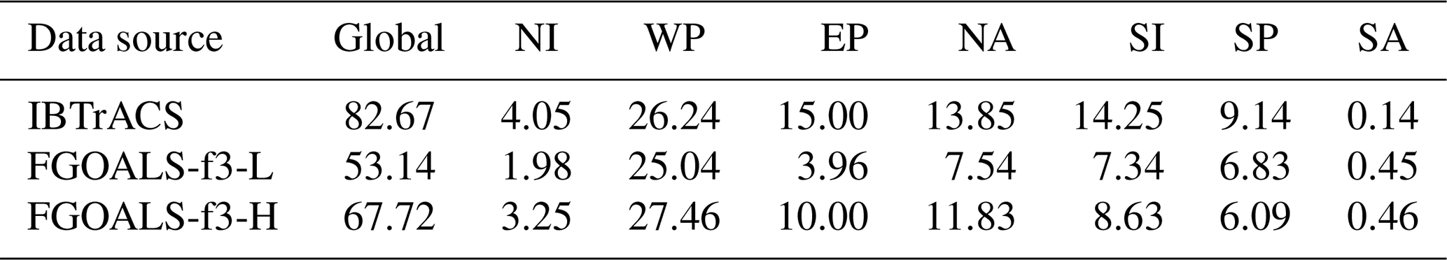
The climatology of simulated tropical cyclones is the first step in testing the performance of the model. Zhao et al. (2009) used a GFDL GCM with a 50 km horizontal resolution to simulate global tropical cyclone activity and obtained a negative bias in the number of tropical cyclones in the eastern Pacific, northern Atlantic and southern Indian oceans. These biases also appeared in the low-resolution models participating in the US Climate Variability and Predictability (CLIVAR) Working Group on Hurricanes (Walsh et al., 2015). Figure 1a and b show the tracks and intensities of global tropical cyclones in the FGOALS-f3-L and FGOALS-f3-H simulations, respectively. The definition of the intensity follows the Saffir–Simpson intensity scale (Simpson and Saffir, 1974). The negative biases of the tracks of tropical cyclones in FGOALS-f3-L (Fig. 1a) improve when the horizontal resolution increases from 100 to 25 km (Fig. 1b) relative to IBTrACS. Table 4 shows the observed and simulated average number of tropical cyclones, both globally and by ocean basin. The results in Table 4 indicate that the value-added effect of tropical cyclone counts from the increased horizontal resolution is seen globally.

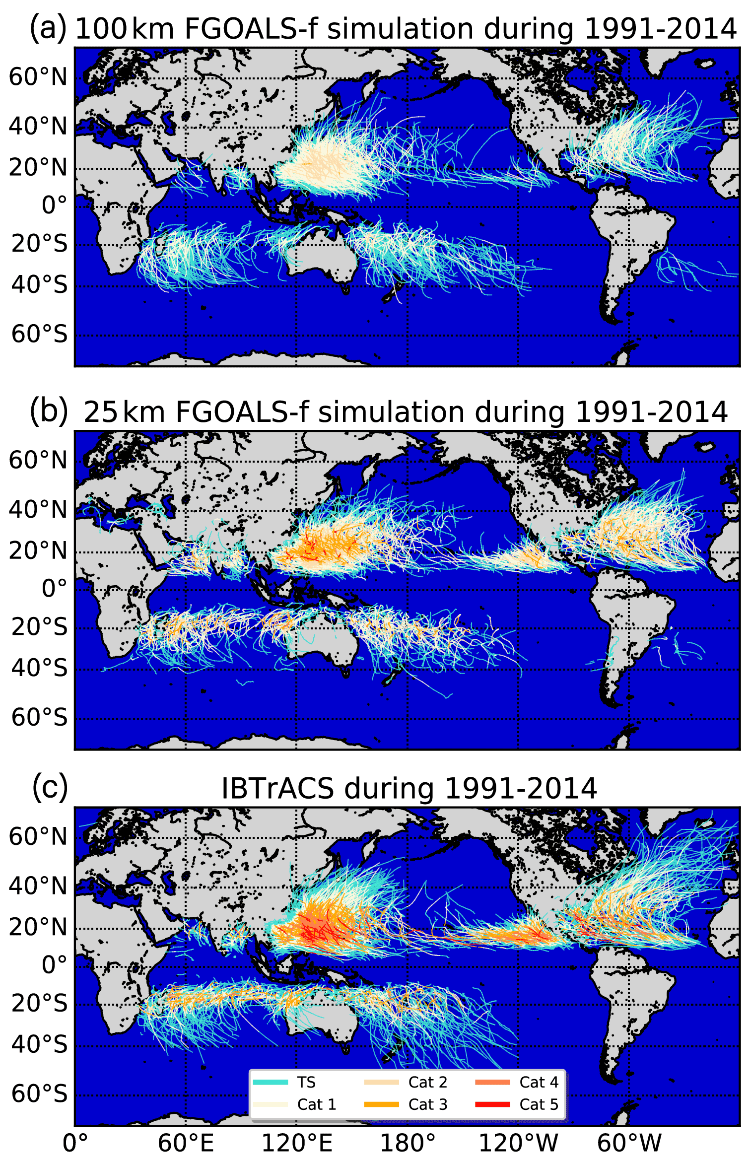
Figure 1 Global tropical cyclone tracks (lines) and intensities (colors) during the time period 1991–2014 between (a) FGOALS-f3-L, (b) FGOALS-f3-H and (c) IBTrACS. The tropical cyclones simulated by FGOALS-f3-L/H are picked out using an objective feature-tracking approach, and only those tropical cyclones with a lifetime >3 d are shown. The definition of intensity threshold is consistent with the Saffir–Simpson scale: TS, tropical storm; Cat 1–5, category 1–5.

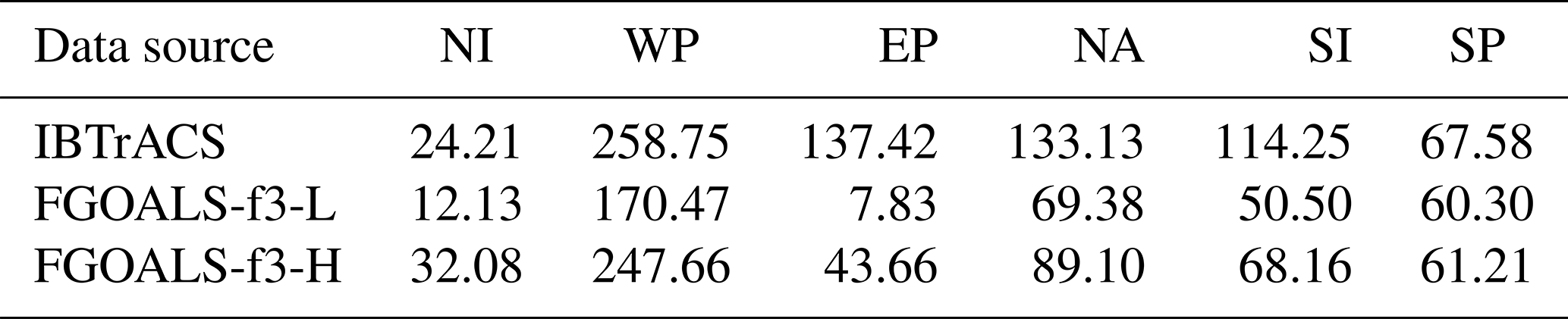
Table 4 Observed and simulated average tropical cyclone number, both globally and by ocean basin, in the northern Indian (NI), western Pacific (WP), eastern Pacific (EP), northern Atlantic (NA), southern Indian Ocean (SI), southern Pacific (SP) and southern Atlantic (SA) oceans.

The improvement is also clearly shown in Fig. 2, and the differences in track densities between FGOALS-f3-H and FGOALS-f3-L reflect a positive distribution in the global basin (Fig. 2c). The biases in the track densities between the simulation and IBTrACS are improved when the horizontal resolution is increased from 100 km (Fig. 2a) to 25 km (Fig. 2b), especially in the low-latitude basins where tropical cyclones form. Negative biases between FGOALS-f3-L and IBTrACS appear in the midlatitudes of the western Pacific and northern Atlantic oceans, but positive biases between the FGOALS-f3-H and IBTrACS also appear in these areas, which means that there are more tropical cyclone events at higher latitudes in FGOALS-f3-H than in IBTrACS and the simulation in FGOALS-f3-L. This phenomenon also exists in the high-resolution GCMs that participated in the European Union Horizon 2020 project PRIMAVERA (Roberts et al., 2020). The biases in the large-scale factors (e.g., strong steering flow) related to the tropical cyclones in GCMs may lead to the simulated biases of tropical cyclone activities in the western Pacific and northern Atlantic oceans.

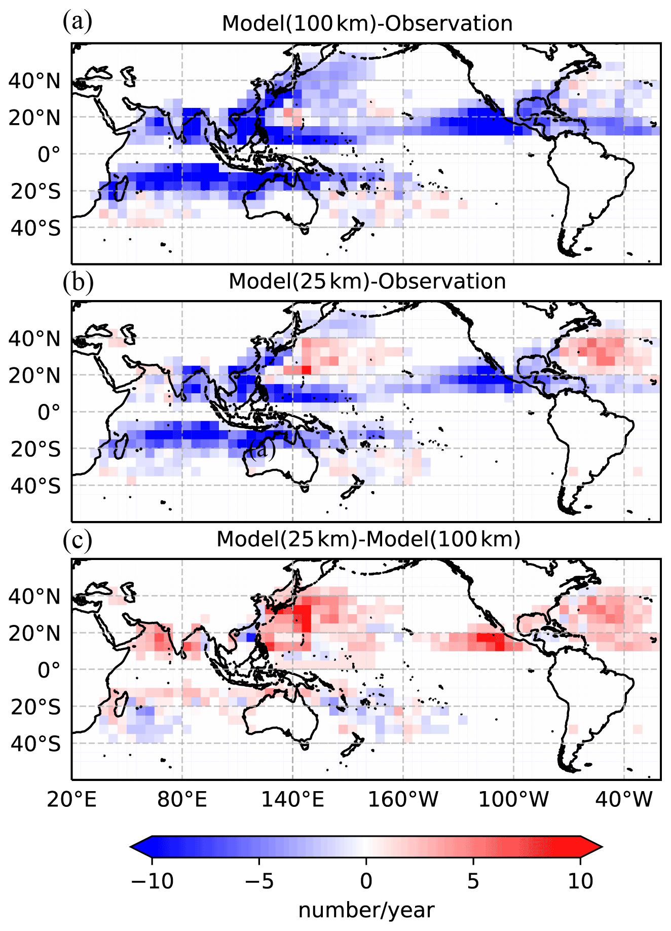
Figure 2 Global track density anomalies of tropical cyclones. The track density is analyzed in (5^∘ × 5^∘) equidistant grid boxes at 6 h intervals and the unit of the color map is the number of cyclones per year from 1991 to 2014. (a) Track density anomaly between FGOALS-f3-L and IBTrACS; (b) track density anomaly between FGOALS-f3-H and IBTrACS; and (c) track density anomaly between FGOALS-f3-H and FGOALS-f3-L.

The negative biases in the intensities of tropical cyclones are also improved when the horizontal resolution is increased from 100 km (Fig. 1a) to 25 km (Fig. 1b), especially in the western Pacific and northern Atlantic oceans. The difference in wind speed densities between FGOALS-f3-L and FGOALS-f3-H (Fig. 3c) shows a significant increase in the wind speed densities in the northern Atlantic, eastern Pacific and northern Indian oceans and the midlatitude region of the western Pacific Ocean when the horizontal resolution is increased from 100 to 25 km. Similar to the pattern of track density anomalies (Fig. 2), the biases in the wind speed densities between FGOALS-f3 and IBTrACS are improved when the horizontal resolution is increased from 100 to 25 km, but the positive biases are intensified in the midlatitudes of the western Pacific and northern Atlantic oceans.

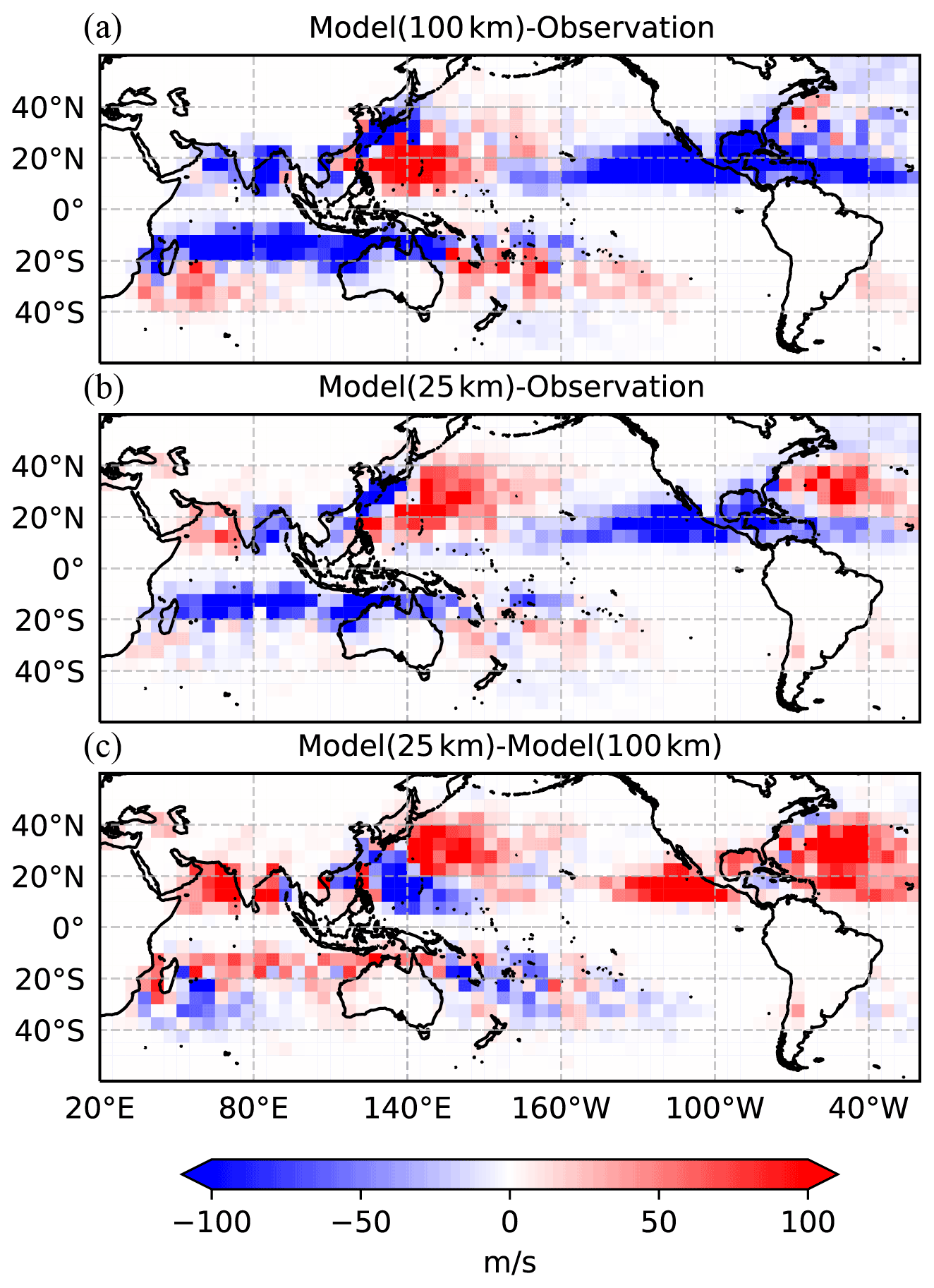
Figure 3 Global maximum sustained wind anomalies of the tropical cyclones (units: m s⁻¹). The track density is analyzed in (5^∘ × 5^∘) equidistant grid boxes at 6 h intervals. (a) Maximum sustained wind anomalies between FGOALS-f3-L and IBTrACS; (b) maximum sustained wind anomalies between FGOALS-f3-H and IBTrACS; and (c) maximum sustained wind anomalies between FGOALS-f3-H and FGOALS-f3-L.

Figure 4 shows the pressure–wind pairs for each 6-hourly measurement of tropical cyclones between FGOALS-f3 and IBTrACS. The results indicate that the simulated intensity of tropical cyclones is increased globally. These results also indicate that the spread of pressure–wind pairs in FGOALS-f3-L is narrow and there is a severe underestimation of intense tropical cyclone events at lower surface pressures and higher wind speeds in the western Pacific and northern Atlantic oceans, although this bias has been dramatically improved (Fig. 4b, d).

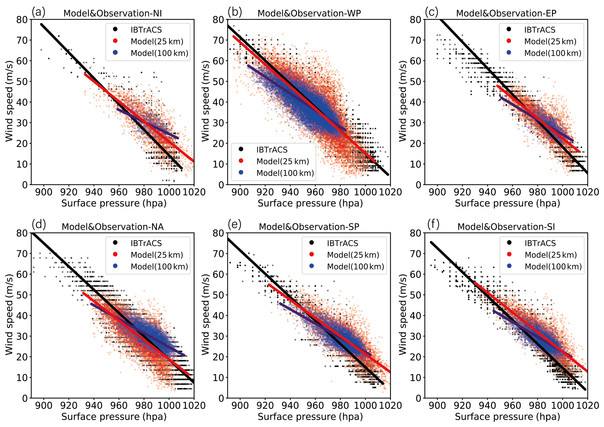
Figure 4 Pressure–wind pairs for each 6-hourly tropical cyclone measurement for FGOALS-f3-L (blue dots) and FGOALS-f3-H (red dots) and IBTrACS (black dots) in the (a) northern Indian Ocean, (b) western Pacific, (c) eastern Pacific, (d) northern Atlantic, (e) southern Pacific and (f) southern Indian oceans. A linear regression (blue/red line for FGOALS-f3-L/H; black line for IBTrACS) is fitted to each distribution of pressure–wind pairs.

The increased intensity of tropical cyclones in FGOALS-f3-H favors the apparent negative bias of the lifetime of tropical cyclones in FGOALS-f3-L when the horizontal resolution is increased. Figure 5 shows the average lifetime of tropical cyclones from 1991 to 2014. The average lifetime of tropical cyclones in the observations is about 8.5, 7.5, 7.5, 4, 6.1 and 7.5 d in the western Pacific, northern Atlantic, eastern Pacific, northern Indian, southern Indian and southern Pacific oceans, respectively, and the simulation of the average lifetime of tropical cyclones is increased in these six basins when the horizontal resolution is increased from 100 to 25 km. For example, the simulated average lifetime of tropical cyclones increases from 6 to 7.4 d when the horizontal resolution is increased in the western Pacific Ocean.

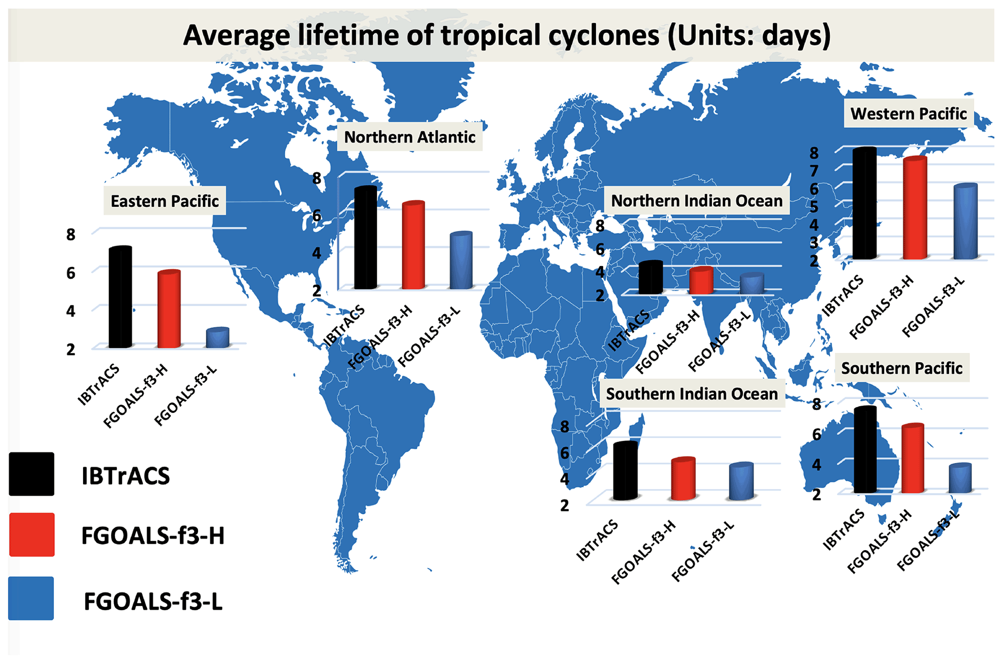
Figure 5 Climatological lifetime of tropical cyclones in the western Pacific, southern Pacific, northern Indian, northern Atlantic, eastern Pacific oceans and southern Indian oceans (units: d) during the time period 1991–2014.

3.2 Seasonal cycles, interannual variability and accumulated cyclone energy of tropical cyclones

Evaluating the seasonal cycle and interannual variability of tropical cyclones in GCMs is an efficient way to verify the coordination between tropical cyclone activity and large-scale circulation patterns (Manganello et al., 2012; Camargo and Wing, 2016; Knutson et al., 2019, 2020). Roberts et al. (2020) found no uniform improvement in the seasonal cycle and interannual variability of tropical cyclones at increased horizontal resolutions, which means that there is a difference in coordination between tropical cyclone activity and large-scale circulation patterns in high-resolution GCMs. Figure 6 shows the seasonal cycle of tropical cyclones between IBTrACS, FGOALS-f3-L and FGOALS-f3-H and shows that FGOALS-f3-L gives a consistent underestimation of the seasonal cycle of tropical cyclones in the northern Atlantic, eastern Pacific, northern Indian, southern Indian and southern Pacific oceans. Neither the single peak in the number of tropical cyclones in the northern Atlantic (peak month September), eastern Pacific (peak month August) and southern Pacific (peak month February) oceans nor the double peak in the northern Indian Ocean (peak months May and November) could be reproduced in FGOALS-f3-L. There are two increases in the simulated number of tropical cyclones in the peak months of the northern Atlantic and eastern Pacific oceans, and the characteristics of the seasonal cycle of simulated tropical cyclones are improved in the northern Indian, western Pacific and southern Pacific oceans as the horizontal resolution is increased from 100 to 25 km. Although FGOALS-f3-H can produce more tropical cyclone counts in the peak month in each basin, both FGOALS-f3-L and FGOALS-f3-H appeared to replicate the timing of the seasonal cycle when we normalized the results of the tropical cyclone seasonal cycle (Fig. A1). Figure 7 shows the interannual correlation of the number of tropical cyclones between FGOALS-f3 and IBTrACS. The results show that the correlation coefficient is improved in each basin, which reflects the fact that the interannual variability between tropical cyclone activity and large-scale circulation patterns is harmonious.

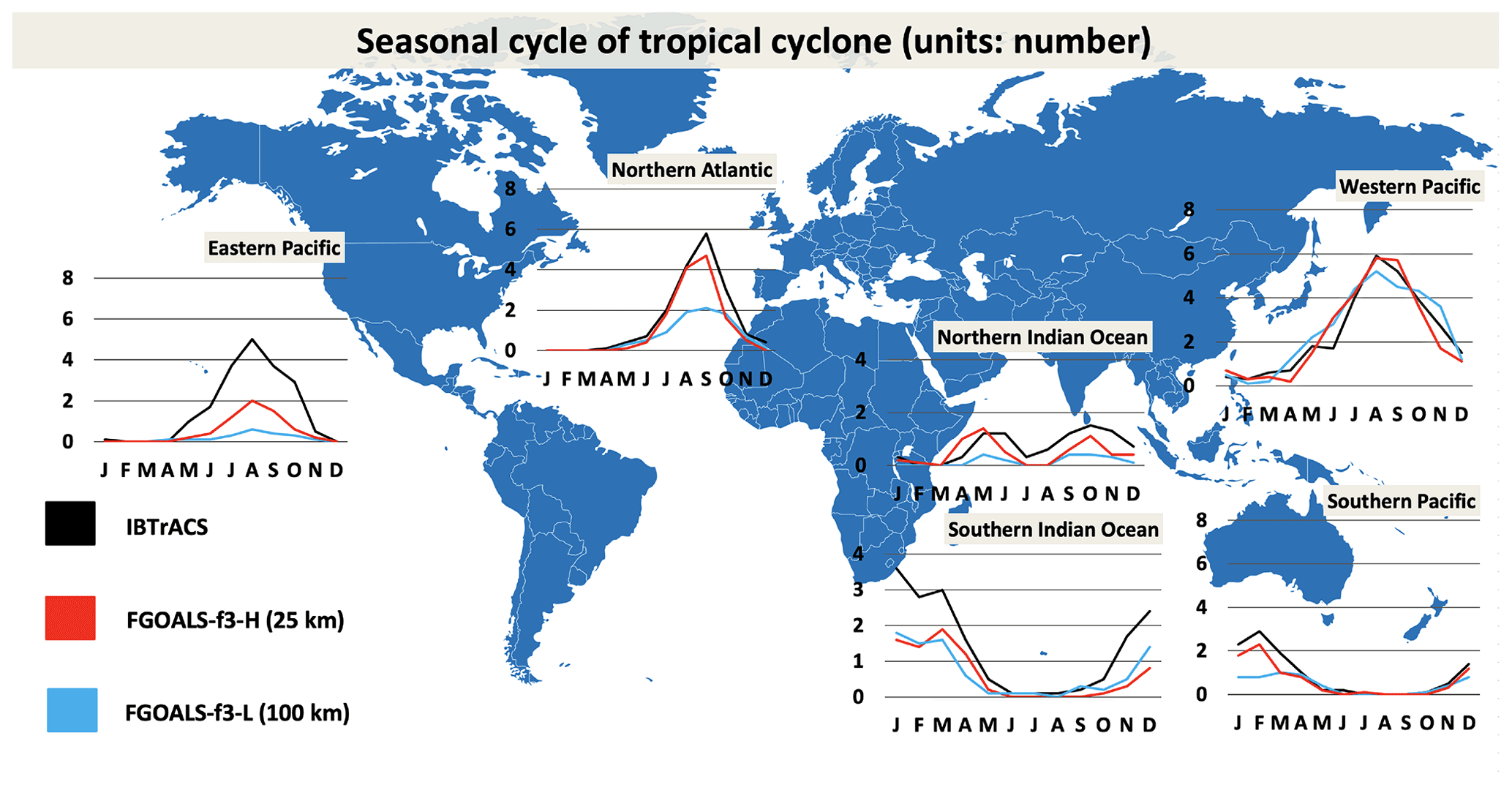
Figure 6 Seasonal cycle of tropical cyclones in the western Pacific, southern Pacific, northern Indian, northern Atlantic, eastern Pacific and southern Indian oceans (units: number of cyclones) during the time period 1991–2014.

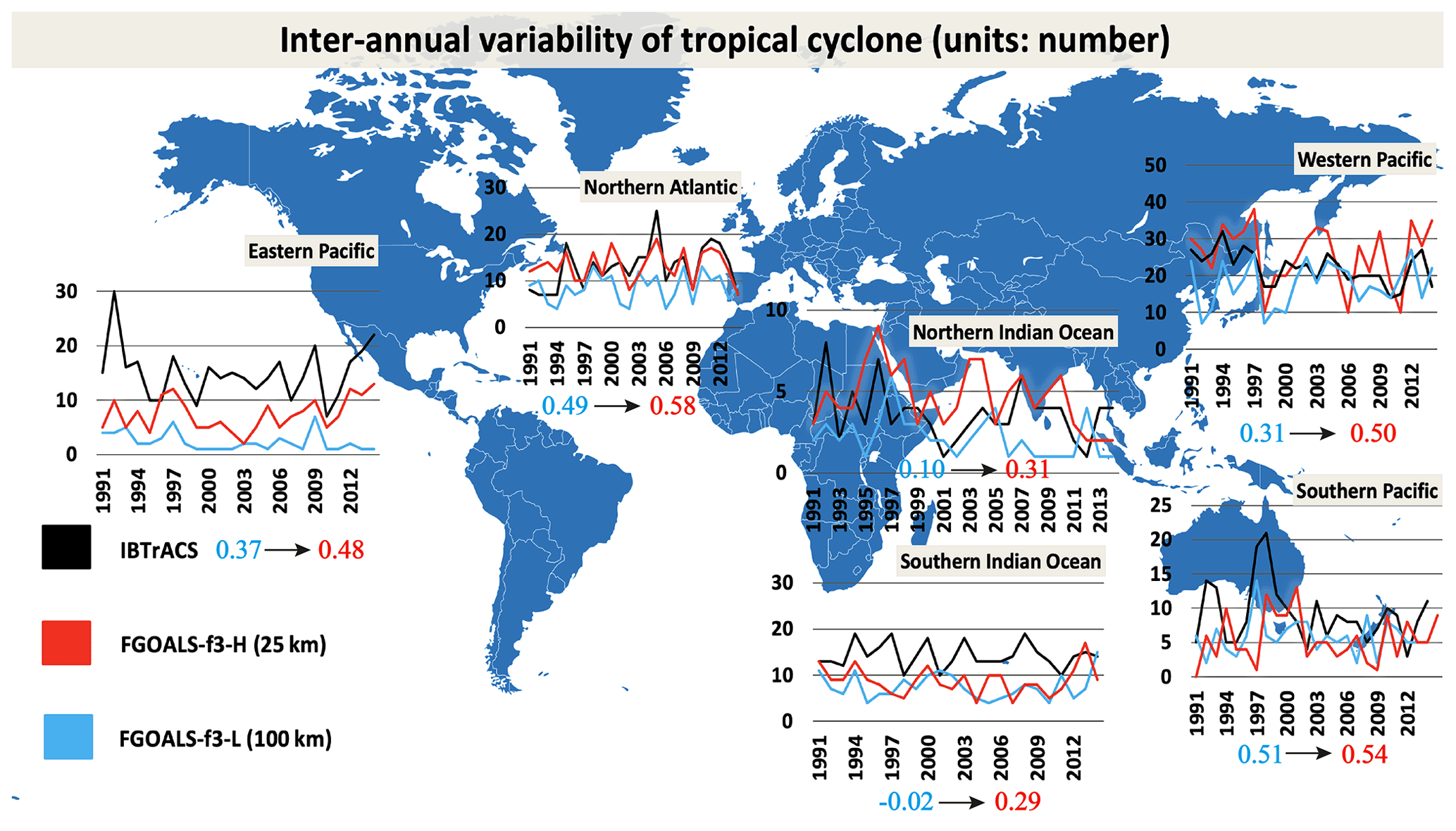
Figure 7 Interannual variability of tropical cyclones in the western Pacific, southern Pacific, northern Indian, northern Atlantic, eastern Pacific and southern Indian oceans (units: number of cyclones) during the time period 1991–2014. The numbers under the line charts are the correlation coefficients between IBTrACS and FGOALS-f3.

Table 5 shows the observed and simulated averaged accumulated cyclone energy (ACE; Bell and Chelliah, 2000). ACE is a measure used by the National Oceanic and Atmospheric Administration in which the energy over the lifetime of a tropical cyclone is calculated for every 6 h period​​​​​​​:

$$\begin{array}{}\text{(1)}& \mathrm{ACE}={\mathrm{10}}^{-\mathrm{4}}\sum V_{\mathrm{m}}^{\mathrm{2}},\end{array}$$

where V_m is the estimated sustained wind speed in knots.

Table 5 Observed and simulated averaged ACE (units: 10⁴ kt) in the northern Indian (NI), western Pacific (WP), eastern Pacific (EP), northern Atlantic (NA), southern Indian (SI) and southern Pacific (SP) oceans.

Our results indicate that the negative biases of the ACE in FGOALS-f3-L are improved globally when the horizontal resolution is increased to 25 km. Figure 8 shows the interannual correlation of the ACE between FGOALS-f3 and IBTrACS. The results show that the correlation coefficient of the ACE between IBTrACS and the simulation is improved in each basin when the horizontal resolution is increased from 100 to 25 km. The increase in the number, lifetime and intensity of simulated tropical cyclones contributes to the increased correlation coefficient of the ACE (Camargo and Sobel, 2005).

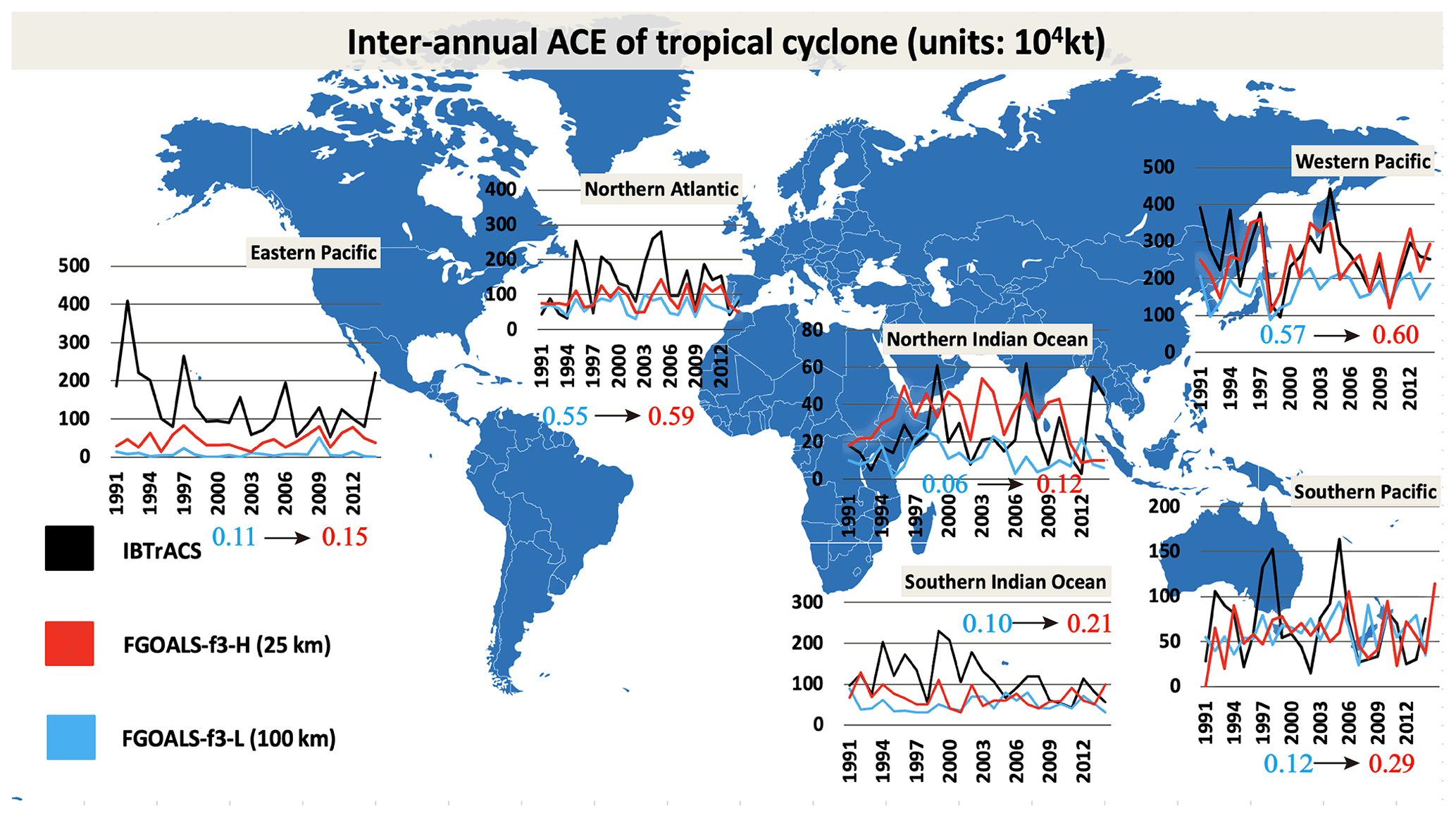
Figure 8 ACE of tropical cyclones (units: 10⁴ kt) in the western Pacific, southern Pacific, northern Indian, northern Atlantic, eastern Pacific, and southern Indian oceans (units: number of cyclones) during the time period 1991–2014.

3.3 Horizontal structure of tropical cyclones

Previous studies have shown that the horizontal resolution influences the horizontal structure of simulated tropical cyclones (Strachan et al., 2013; Murakami et al., 2012, 2013; Roberts et al., 2020). Manganello et al. (2012) compared the horizontal structure of the moisture content of tropical cyclones in GCMs between low (T511) and high (T2047) resolutions and found that the refined structure of the liquid component of tropical cyclones was simulated when the horizontal resolution was increased. Following the method of Manganello et al. (2012), the surface 10 m wind and daily precipitation rate for the 30 most intense tropical cyclones in FGOALS-f3-L (Fig. 9a) and FGOALS-f3-H (Fig. 9b) were combined. The results of the GFS (Fig. 9c) and the GFS and GPM (Fig. 9d) simulations are also shown for comparison. The results indicate that there is no prominent precipitation structure of tropical cyclones in FGOALS-f3-L, but there is a considerable improvement in the results with a horizontal resolution of 25 km. The eyewall and organized precipitation of tropical cyclones are apparent in the FGOALS-f3-H simulation. The main uncertainty is the position of extreme precipitation. The position of extreme precipitation appears 100 km east of the eyewall in the FGOALS-f3-H simulation (Fig. 9b) but is 100 km south of the eyewall in the GFS and GPM datasets (Fig. 9c). There is an apparent error in the angle compared with the radial distance for the simulated horizontal structure of tropical cyclones. Chen et al. (2006) found that the vertical wind shear and storm motion are the two most important factors contributing to rainfall asymmetries in tropical cyclones. The biases in the vertical wind shear and storm motion in FGOALS-f3 may affect the angle of the horizontal structure of tropical cyclones. The non-hydrostatic dynamical core used in FGOALS-f3 and the limited air–sea coupling processes (Emanuel and Sobel, 2013; Kim et al., 2018) (AMIP) also contribute to the error.

Figure 9 Surface 10 m winds (units: m s⁻¹) and daily precipitation rate (mm d⁻¹) for the horizontal composite of the 30 most intense tropical cyclones in (a) FGOALS-f3-L and (b) FGOALS-f3-H. (c) Results of the surface 10 m wind in GFS and the daily precipitation rate in GPM. Radius is 4^∘.

4 Possible reasons for the simulated performance of tropical cyclones in FGOALS-f3

4.1 Modulation of tropical cyclone activity by the ENSO

There is a lot of evidence to suggest that the ENSO modulates the activity of tropical cyclones. Gray (1984) found that tropical cyclone counts in the Atlantic Ocean are modulated by the ENSO. El Niño (La Niña) events enhanced (suppressed) westerly winds and led to stronger (weaker) vertical wind shear in the Atlantic basin, leading to an increase (decrease) in tropical cyclone counts. Camargo and Sobel (2005) found that the ACE in the western Pacific is positively correlated with ENSO indices. There are more intense and longer-lived tropical cyclones in El Niño years than in La Niña years. Kim et al. (2011) found that the ENSO modulates tropical cyclone activity in the eastern Pacific Ocean. The track densities and genesis of tropical cyclones tend to be enhanced (suppressed) in eastern Pacific warming (cooling) years by strong (weak) westerly wind shear.

Figure 10 shows the average number of tropical cyclones and the ACE from El Niño, neutral and La Niña years. In the western Pacific basin (Fig. 10a), there is no clear change in tropical cyclone counts compared with the variation of the ACE between El Niño and La Niña years. FGOALS-f3-H can capture these features in the observations; in particular, the simulation of the ACE is better than in FGOALS-f3-L. In the eastern Pacific basin (Fig. 10b), FGOALS-f3 can capture the variation in tropical cyclone activities from El Niño to La Niña years, but the decreasing trend of tropical cyclone counts and the ACE in FGOALS-f3-L/H is weaker than in the observations. In the observations for the northern Atlantic basin (Fig. 10c), there are more intense tropical cyclone events in La Niña years. FGOALS-f3 can reproduce the impact of the ENSO on tropical cyclone activity in the northern Atlantic Ocean and the simulated performance of tropical cyclones in FGOALS-f3-H is better than that in FGOALS-f3-L.

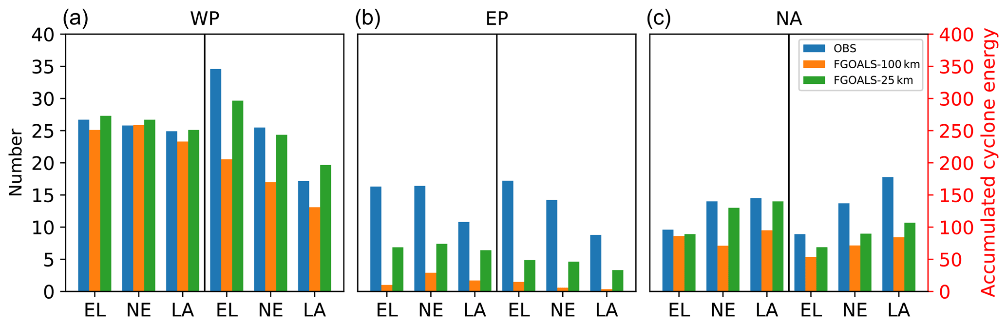
Figure 10 Bar chart showing the average number of tropical cyclones (left-hand panels) and ACE (right-hand panels) from El Niño (EL), neutral (NE) and La Niña (LA) years in the (a) western Pacific (WP), (b) eastern Pacific (EP) and (c) northern Atlantic (NA) oceans.

4.2 Large-scale environmental factors

The genesis potential index (GPI; Emanuel et al., 2004) is applied to detect the connection between the genesis of tropical cyclones and large-scale circulation patterns. Camargo et al. (2007) and Walsh et al. (2013) found that the correlation between the GPI and the variation of tropical cyclones in GCMs mainly depends on the horizontal resolution and the similarity between the GPI. The variation in tropical cyclones is increased when the horizontal resolution is increased. The GPI used in this work is defined as

$$\begin{array}{}\text{(2)}& \mathrm{GPI}={\left|{\mathrm{10}}^{\mathrm{5}}\mathrm{vort}\mathrm{850}\right|}^{\mathrm{3}/\mathrm{2}}\left({\displaystyle \frac{\mathrm{RH}}{\mathrm{50}}}\right)\left({\displaystyle \frac{V_{\mathrm{m}}}{\mathrm{70}}}\right){\left(\mathrm{1}+\mathrm{0.1}{V}_{\mathrm{shear}}\right)}^{-\mathrm{2}},\end{array}$$

where vort850 is the 850 hPa absolute vorticity (s⁻¹), RH is the 600 hPa relative humidity (%), V_m is the maximum potential intensity (Emanuel, 1995), and V_shear is the magnitude of the wind shear between 850 and 200 hPa (m s⁻¹). V_m (the maximum potential intensity) is defined here as

$$\begin{array}{}\text{(3)}& V_{\mathrm{m}}={\displaystyle \frac{C_{\mathrm{k}}{T}_{\mathrm{s}}}{C_{\mathrm{d}}{T}_{\mathrm{0}}}}\left({\mathrm{CAPE}}^{*}-{\mathrm{CAPE}}^{\mathrm{b}}\right),\end{array}$$

where C_k is the exchange coefficient of the enthalpy, C_d is the drag coefficient, T_s is the sea surface temperature, and T₀ is the mean outflow temperature. CAPE^* is the convective available potential energy of the air lifted from saturation at sea level and CAPE^b is the convective available potential energy of the boundary layer air.

Figure 11 shows the biases of the large-scale environmental factors related to tropical cyclone activity between FGOALS-f3 and the observations. The results indicate that the biases in the large-scale environmental factors are decreased in FGOALS-f3 when horizontal resolution is increased from 100 to 25 km, which is related to the biases in the simulated tropical cyclones. For example, the environmental vertical wind shear (VWS) is known to be one of the major factors in the generation and intensity of tropical cyclones (Gray, 1968; Wong and Chan, 2004). An excessive VWS in the eastern Pacific and northern Atlantic oceans can lead to the suppression of the generation and intensity of simulated tropical cyclones in these basins (Fig. 11e), which is consistent with the results for the simulation of tropical cyclones in FGOALS-f3-L (Fig. 3). The results in Fig. 12 show the pattern correlation of each individual part of the GPI. P1 represents the equation ${\left|{\mathrm{10}}^{\mathrm{5}}\mathrm{vort}\mathrm{850}\right|}^{\mathrm{3}/\mathrm{2}}$, P2 represents the equation $\frac{\mathrm{RH}}{\mathrm{50}}$, P3 represents the equation $\frac{V_{\mathrm{m}}}{\mathrm{70}}$ and P4 represents the equation ${\left(\mathrm{1}+\mathrm{0.1}{V}_{\mathrm{shear}}\right)}^{-\mathrm{2}}$. The results indicate that the pattern correlation coefficients are increased in the northern Indian (Fig. 12a), western Pacific (Fig. 12b), eastern Pacific (Fig. 12c) and northern Atlantic (Fig. 12d) oceans, which is favored by the reduction in the bias of the large-scale circulation patterns.

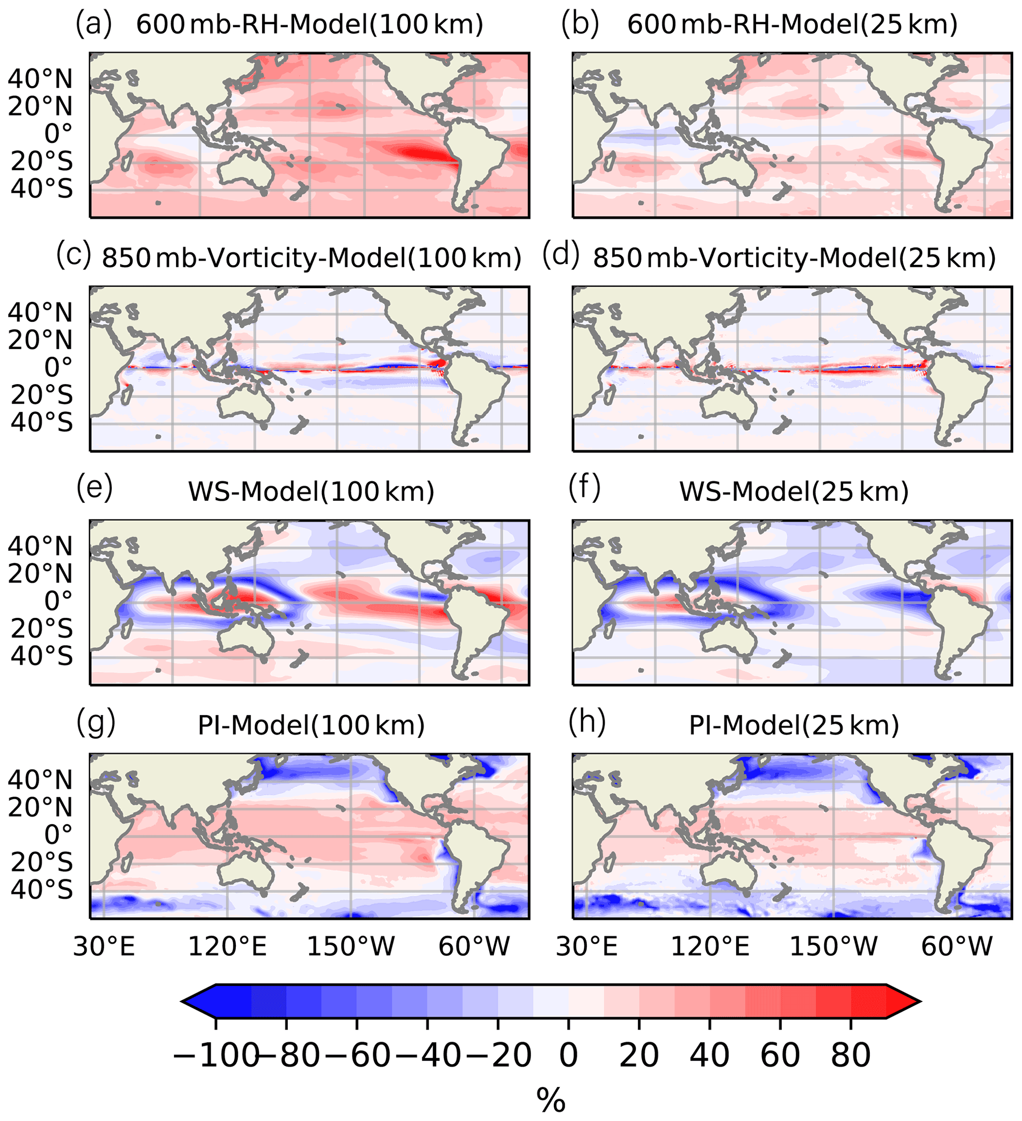
Figure 11 Biases in the large-scale environmental factors related to tropical cyclone activity between FGOALS-f3 and the observations. (a, b) Relative humidity biases at 600 hPa; (c, d) absolute vorticity biases at 850 hPa; (e, f) wind shear biases between 200 and 850 hPa; and (g, h) potential intensity biases.

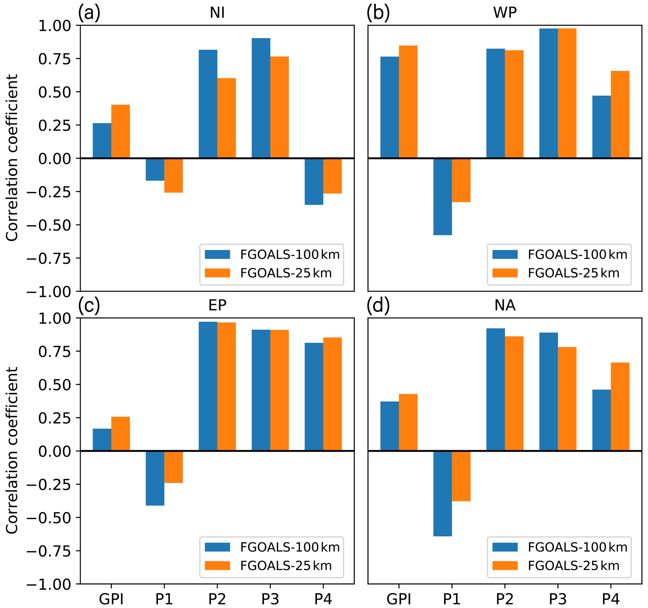
Figure 12 Pattern correlation of annual tropical cyclone GPI between the ERA-Interim dataset and the simulation of FGOALS-f3 at low (blue bars) and high (orange bars) horizontal resolutions in the (a) northern Indian, (b) western Pacific, (c) eastern Pacific and (d) northern Atlantic oceans. P1–P4 represent parts 1–4 of Eq. (2). P1 represents the equation $|{\mathrm{10}}^{\mathrm{5}}\mathrm{vort}\mathrm{850}{|}^{\mathrm{3}/\mathrm{2}}$, P2 represents the equation $\frac{\mathrm{RH}}{\mathrm{50}}$, P3 represents the equation $\frac{V_{\mathrm{m}}}{\mathrm{70}}$, and P4 represents the equation ${\left(\mathrm{1}+\mathrm{0.1}{V}_{\mathrm{shear}}\right)}^{-\mathrm{2}}$.

5 Discussion

5.1 Impact of physical parameterization and air–sea coupling on tropical cyclones simulated in GCMs

An RCP scheme has been used in both the high- and low-resolution versions of FGOALS-f3 (Bao and Li, 2020; He et al., 2019; Li et al., 2019). The RCP scheme calculates convective and stratiform precipitation at the grid scale, which has the advantage of both scale awareness and high computational efficiency. The parameterizations of physical processes in traditional GCMs are very sensitive to changes in resolution. In particular, convection and cloud processes are considered to be effectively resolved, which means that the assumptions and equations in low-resolution simulations are not suitable for high-resolution GCMs. As a result, the model convergence will be degraded as the resolution increases (Sakradzija et al., 2016). Simulated tropical cyclones are very sensitive to convection and cloud processes in GCMs (Zhao et al., 2012). The effective tuning of convection (Lim et al., 2015; Murakami et al., 2012), boundary condition (Zhang et al., 2017) and microphysics (Chutia et al., 2019) parameterizations contributes to improvements in the intensity, number, track and structure of simulated tropical cyclone. Although a fixed parameterization scheme combined with a fine grid will clearly improve the simulation of tropical cyclone activity, the effect of resolution will be amplified. According to this study, GCMs with scale-aware parameterizations still slightly underestimate the intensity of tropical cyclones at 0.25^∘ resolution (Fig. 1). In addition, air–sea exchange and non-hydrostatic processes are both important in enhancing the intensity of tropical cyclones (Ma et al., 2017). Emanuel and Sobel (2013) found that the absence of air–sea coupling can lead to potentially large imbalances in the surface energy budget, which is not conducive to the development of tropical cyclones.

5.2 Large-scale environmental factors from HighResMIP models

Our results (Fig. 11) show a clear improvement in the large-scale factors related to the generation and development of tropical cyclones when the horizontal resolution is increased from 100 to 25 km in FGOALS-f3. It is worth exploring whether these improved large-scale factors are common to all the GCMs participating in HighResMIP. The eight models participating in HighResMIP Tier 1 were selected (Table 6) to calculate the GPI. The results indicate that the GPI patterns in high-resolution models (Fig. 13b) are closer to the observations (Fig. 13a) than those in the standard-resolution models (Fig. 13c), which means that the large-scale factors related to tropical cyclones are improved when the horizontal resolution of the models is increased. However, the differences between the tracking algorithms – such as TRACK (Hodges et al., 2017), TSTORM (Zhao et al., 2009) and TempestExtremes (Ullrich and Zarzycki, 2017; Ullrich et al., 2021) – are also an important factor in the uncertainties in tropical cyclone simulations. Cross validation of the performance of tropical cyclone simulations with multiple tracking algorithms is necessary in future research (Roberts et al., 2020).

Table 6 Information about the GCMs participating in HighResMIP.

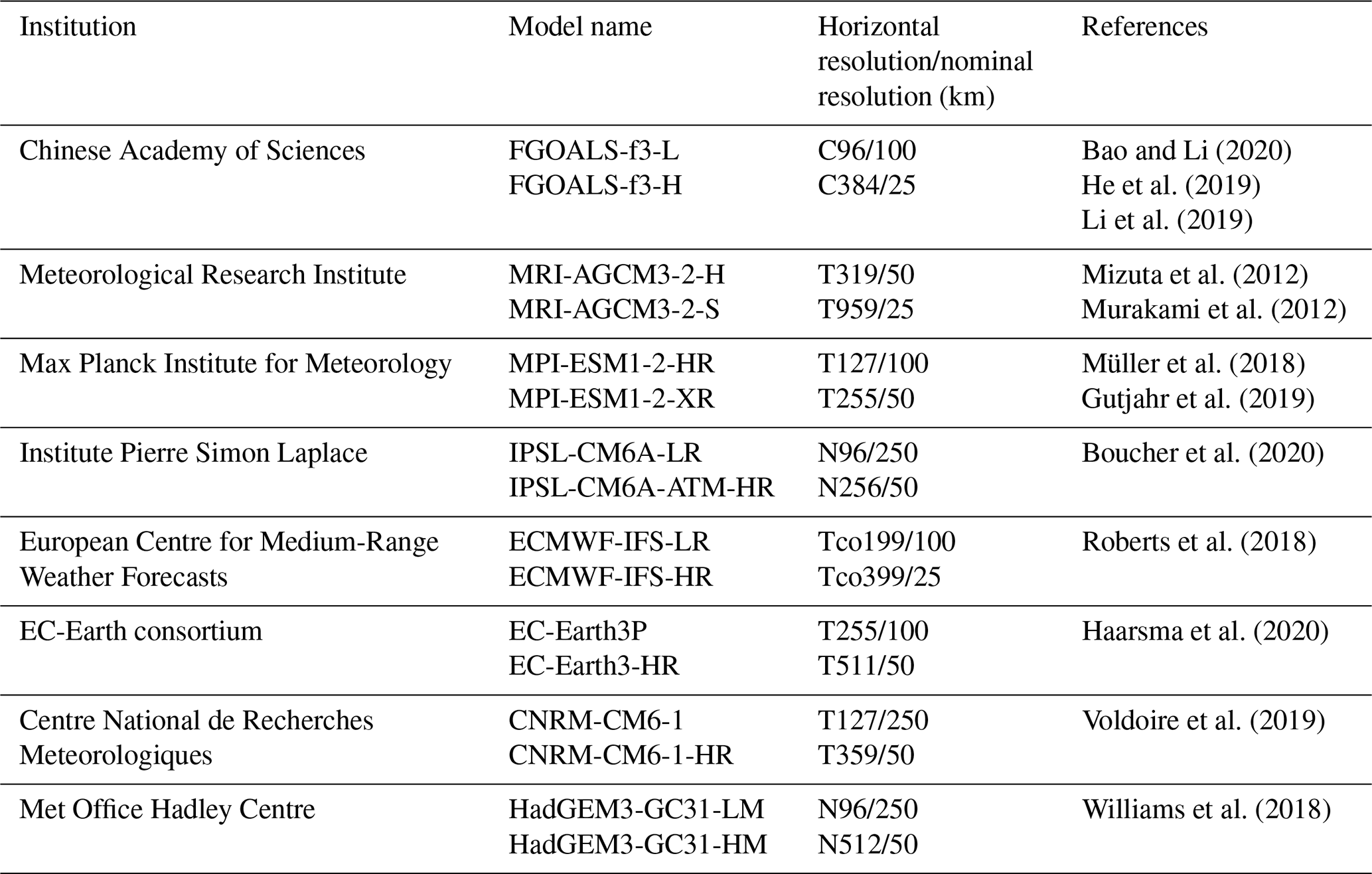
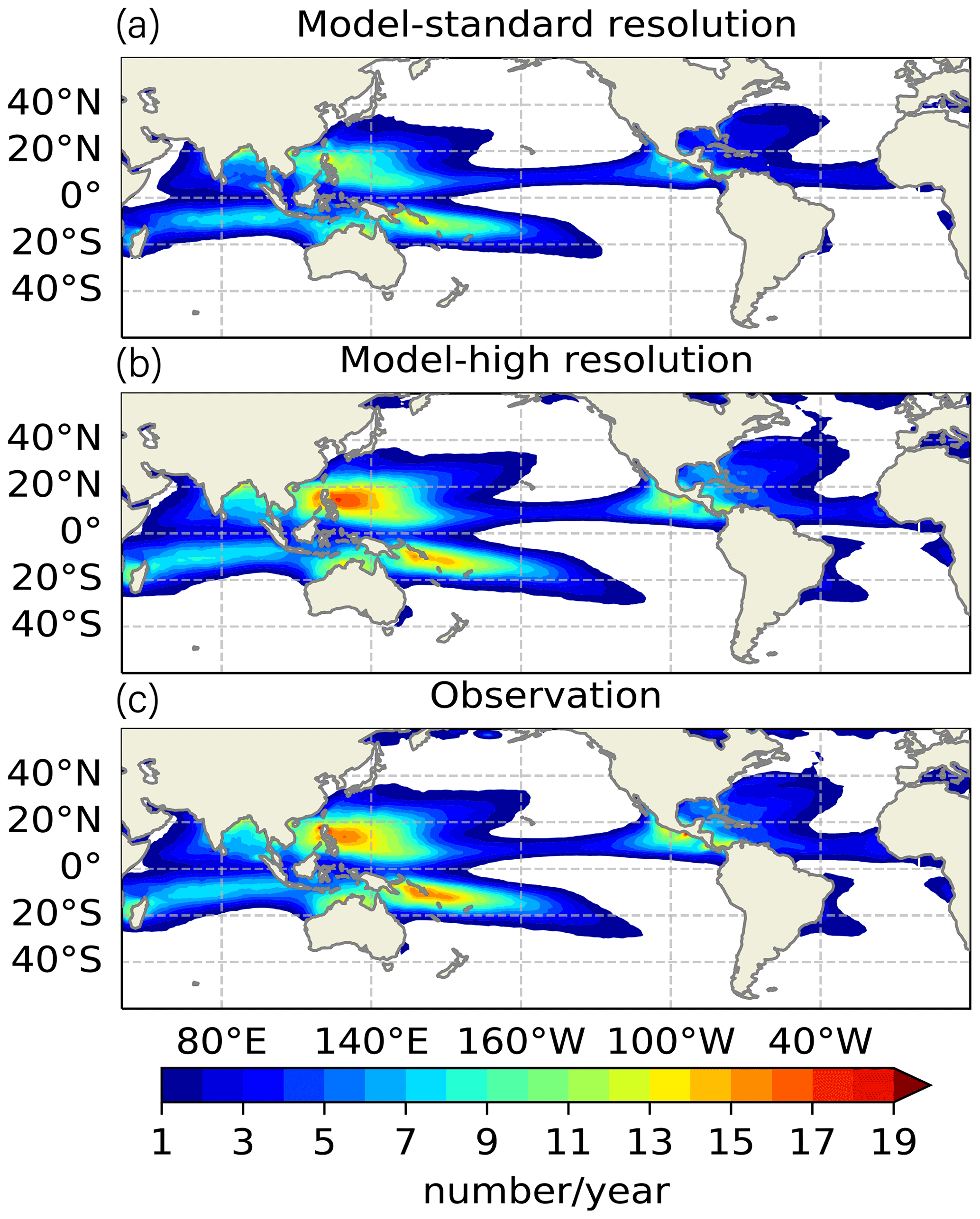
Figure 13 Global GPI pattern based on the multi-model mean of the (a) standard-resolution GCMs and (b) high-resolution GCMs and (c) ERA-Interim dataset.

6 Summary and conclusions

The impacts of horizontal resolution on the simulation of tropical cyclones were studied with the latest version of FGOALS-f3, which participated in the CMIP6 HighResMIP (Haarsma et al., 2016). Li et al. (2019) evaluated the simulation performance of tropical cyclone activity in FAMIL2 (resolution about 100 km), which is the atmospheric component of FGOALS-f3 (He et al., 2019) and put forward the idea that the simulated performance of tropical cyclones is improved with the increased horizontal resolution in FAMIL2. We examined these hypotheses and our main findings and conclusions are as follows.

1. There are improvements in the track and intensity of global tropical cyclones in the FGOALS-f3 simulations when the horizontal resolution is increased from 100 (FGOALS-f3-L) to 25 km (FGOALS-f3-H) and the negative biases in tropical cyclone genesis are improved in the eastern Pacific and northern Atlantic oceans. Quantitative comparisons between the track density of tropical cyclones between FGOALS-f3-L, FGOALS-f3-H and IBTrACS show that the negative biases in the tropical cyclone track densities at low latitudes are alleviated. The surface wind speed of tropical cyclones is increased when the horizontal resolution is increased and this change in FGOALS-f3-H is closer to the observations. The improvement in the intensity of tropical cyclones in FGOALS-f3-H is easier to detect in the pressure–wind pairs of tropical cyclones. A wide spread of pressure–wind pairs is simulated in FGOALS-f3-H and the biases in the pressure–wind pairs are improved relative to the observations.

2. The global lifetimes of tropical cyclones in FGOALS-f3-H are increased compared with the FGOALS-f3-L simulation, especially in the western Pacific, northern Atlantic, eastern Pacific and southern Pacific oceans. The increase in the intensity of tropical cyclones in FGOALS-f3-H contributes to the improvement in the lifetime of tropical cyclones. In the seasonal cycle of tropical cyclones, only 50 % of tropical cyclones are simulated in the peak month, but this bias is improved in FGOALS-f3-H compared with the observations. Both FGOALS-f3-L and FGOALS-f3-H appear to replicate the timing of the seasonal cycle. The average ACE and number of tropical cyclones in FGOALS-f3-H are close to the observations. The correlation of the annual number of tropical cyclones and the annual ACE of tropical cyclones are both improved in the western Pacific, northern Atlantic, eastern Pacific, southern Pacific and northern Indian oceans when the horizontal resolution is increased.

3. There is a significant improvement in the horizontal structure of tropical cyclones in FGOALS-f3 when the horizontal resolution is increased. The eyewall and the organized precipitation of tropical cyclones are apparent in the FGOALS-f3-H simulation and the main uncertainty is the position of extreme precipitation.

4. The possible reasons for the improvement in the simulated tropical cyclones are explained by the ENSO and large-scale environmental factors. FGOALS-f3 can reproduce the response between the ENSO and tropical cyclone activities, and the biases in the number of tropical cyclones and the ACE in FGOALS-f3-H are decreased. The large-scale factors and GPI biases between FGOALS-f3-L and FGOALS-f3-H are consistent with the biases in the simulated tropical cyclones, which means that the improvement in the large-scale environmental factors in FGOALS-f3 contributes to the simulation of tropical cyclones. This study shows that it is worth establishing a high-resolution coupled dynamic prediction system based on FGOALS-f3-H to improve the prediction skill of tropical cyclones on subseasonal to seasonal scales (Camp et al., 2019; Murakami et al., 2016). This dataset will be uploaded to the subseasonal to seasonal prediction project (Vitart and Robertson, 2018; Vitart et al., 2017).

Appendix A

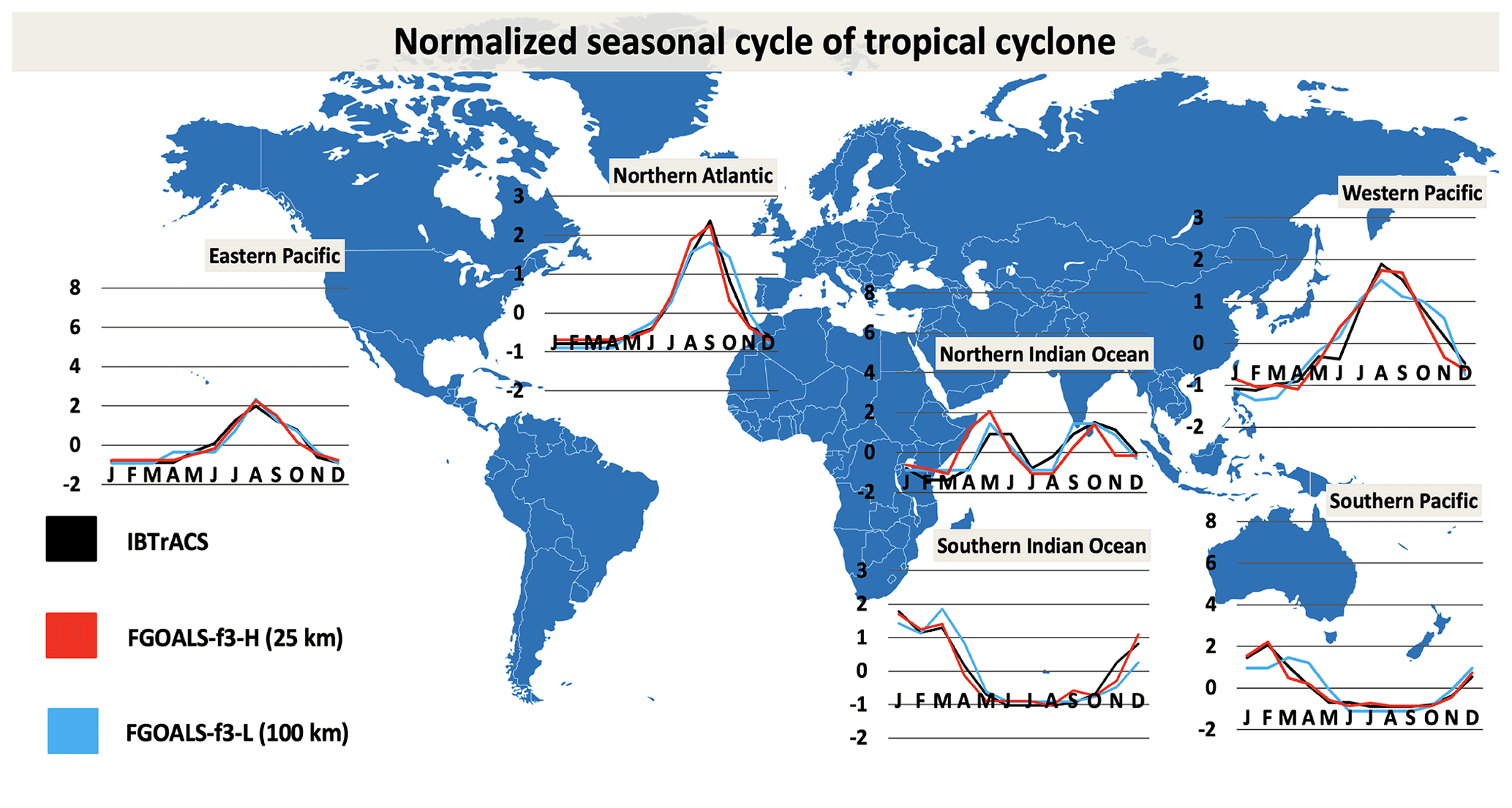
Figure A1 Seasonal cycle of tropical cyclones with zero-mean normalization in the western Pacific, southern Pacific, northern Indian, northern Atlantic, southern Indian and eastern Pacific oceans (units: number of cyclones) during the time period 1991–2014.