Incorporation of volcanic SO₂ emissions in the Hemispheric CMAQ (H-CMAQ) version 5.2 modeling system and assessing their impacts on sulfate aerosol over the Northern Hemisphere

The state-of-the-science Community Multiscale Air Quality (CMAQ) Modeling System has recently been extended for hemispheric-scale modeling applications (referred to as H-CMAQ). In this study, satellite-constrained estimation of the degassing SO₂ emissions from 50 volcanoes over the Northern Hemisphere is incorporated into H-CMAQ, and their impact on tropospheric sulfate aerosol (${\mathrm{SO}}_{\mathrm{4}}^{\mathrm{2}-}$) levels is assessed for 2010. The volcanic degassing improves predictions of observations from the Acid Deposition Monitoring Network in East Asia (EANET), the United States Clean Air Status and Trends Network (CASTNET), and the United States Integrated Monitoring of Protected Visual Environments (IMPROVE). Over Asia, the increased ${\mathrm{SO}}_{\mathrm{4}}^{\mathrm{2}-}$ concentrations were seen to correspond to the locations of volcanoes, especially over Japan and Indonesia. Over the USA, the largest impacts that occurred over the central Pacific were caused by including the Hawaiian Kilauea volcano, while the impacts on the continental USA were limited to the western portion during summertime. The emissions of the Soufrière Hills volcano located on the island of Montserrat in the Caribbean Sea affected the southeastern USA during the winter season. The analysis at specific sites in Hawaii and Florida also confirmed improvements in regional performance for modeled ${\mathrm{SO}}_{\mathrm{4}}^{\mathrm{2}-}$ by including volcanoes SO₂ emissions. At the edge of the western USA, monthly averaged ${\mathrm{SO}}_{\mathrm{4}}^{\mathrm{2}-}$ enhancements greater than 0.1 µg m⁻³ were noted within the boundary layer (defined as surface to 750 hPa) during June–September. Investigating the change on ${\mathrm{SO}}_{\mathrm{4}}^{\mathrm{2}-}$ concentration throughout the free troposphere revealed that although the considered volcanic SO₂ emissions occurred at or below the middle of free troposphere (500 hPa), compared to the simulation without the volcanic source, ${\mathrm{SO}}_{\mathrm{4}}^{\mathrm{2}-}$ enhancements of more than 10 % were detected up to the top of the free troposphere (250 hPa). Our model simulations and comparisons with measurements across the Northern Hemisphere indicate that the degassing volcanic SO₂ emissions are an important source and should be considered in air quality model simulations assessing background ${\mathrm{SO}}_{\mathrm{4}}^{\mathrm{2}-}$ levels and their source attribution.

1 Introduction

Airborne sulfate (${\mathrm{SO}}_{\mathrm{4}}^{\mathrm{2}-}$) is one of the major components of tropospheric particulate matter worldwide (Zhang et al., 2007) and plays important roles in modulating the earth–atmosphere energy budget, atmospheric circulation, cloud properties, and precipitation (Seinfeld and Pandis, 2016). ${\mathrm{SO}}_{\mathrm{4}}^{\mathrm{2}-}$ is produced via the aqueous- and gas-phase oxidation of sulfur dioxide (SO₂), and these processes are well understood (Seinfeld and Pandis, 2016). The dominant sources of SO₂ emissions are attributed to anthropogenic activity (Warneck and Williams, 2012). The global anthropogenic SO₂ emissions peaked in the early 1970s with around 130 Tg yr⁻¹ and then decreased; however, this emission trend has contrasting characteristics over the USA and Asia (e.g., Smith et al., 2011; Xing et al., 2015a). Anthropogenic SO₂ emissions from the USA showed a peak in the early 1970s with 30 Tg yr⁻¹ and subsequently decreased (Smith et al., 2011). Publicly available observational records have begun from the late 1980s over the USA, and it has been confirmed that ${\mathrm{SO}}_{\mathrm{4}}^{\mathrm{2}-}$ concentration in the USA decreased during the early 1990s through 2010 in response to these reductions in SO₂ emissions as evidenced in analyses of observational aerosol composition (e.g., Hand et al., 2012; Gan et al., 2015). On the other hand, anthropogenic SO₂ emissions across Asia, especially China, have shown a continuous increase since 1970 (Smith et al., 2011) up to 2006 and then decreased (Li et al., 2017) in response to control measures. These multi-decadal changes in SO₂ emissions have resulted in not only contrasting changes in tropospheric ${\mathrm{SO}}_{\mathrm{4}}^{\mathrm{2}-}$ levels but also in aerosol radiative effects (e.g., Wild et al., 2009; Xing et al., 2015b), their feedback on atmospheric dynamics and air quality (e.g., Xing et al., 2016), and acid deposition (e.g., Zhang et al., 2018; Mathur et al., 2020).

As SO₂ emission control is reducing regional airborne ${\mathrm{SO}}_{\mathrm{4}}^{\mathrm{2}-}$, quantifying the relative contribution of long-range transported ${\mathrm{SO}}_{\mathrm{4}}^{\mathrm{2}-}$ and the portion attributable to natural sources is becoming increasingly important. For instance, regional haze assessments require quantification of visibility impairment that are associated with anthropogenic enhancements over natural visibility levels, which in turn necessitates accurate quantification of the contribution of natural sources. Next to the anthropogenic emissions, volcanic emissions have an important contribution to SO₂ emissions (Warneck and Williams, 2012). A time-averaged inventory of volcanic emissions was estimated as 13 Tg SO₂ yr⁻¹ during the early 1970s to 1997, and these volcanoes are mostly located in the Pacific Rim region (Andres and Kasgnoc, 1998). Volcanic emission fluxes can be measured in several ways such as a correlation spectrometer (COSPEC), but observable volcanic eruptions are limited in time and location. Satellite observations are now proving to be a useful approach to monitor the volcanic emissions and have provided a global volcanic SO₂ emission inventory since 1978 (Carn et al., 2016). Accurate representation of volcanic emissions requires quantification of emissions emitted from both persistent degassing and sporadic eruptions. Recently, a decadal-scale global volcanic SO₂ emissions inventory for the 2005–2015 period, constrained by the Ozone Monitoring Instrument (OMI), has been established (Carn et al., 2017). The enhanced methodology with greater sensitivity allows the detection of emissions as low as approximately 6 Gg SO₂ yr⁻¹ for low-altitude volcanoes and covers a total of 91 persistently degassing volcanic SO₂ sources. The volcanic SO₂ emissions from degassing are relatively stable at 23.0±2.3 Tg SO₂ yr⁻¹ during 2005–2015, and the highest amount was approximately 26 Tg SO₂ yr⁻¹ in 2010. In terms of the volcanic activity, sporadic eruptions inject into the atmosphere comparatively large amounts of SO₂ emissions. For example, one of the largest eruptions in the 1990s was that of Mt. Pinatubo in June 1991, which was estimated to have injected 18 Tg of SO₂ emissions into the atmosphere (Smithsonian Institution, 2020). The injection heights of that eruption reached to more than 30 km and caused the largest perturbations ever observed in the chemical state of the stratosphere and the earth–atmosphere radiation budget (McCormick, et al., 1995). However, such eruptive emissions are temporary. According to the comparison between the degassing and eruptive emissions, Carn et al. (2017) estimated that during 2005–2015, volcanic activity contributed about 23 Tg yr⁻¹ of SO₂ due from degassing while eruptive SO₂ emissions ranged from 0.2 to 10 Tg yr⁻¹ of SO₂. Therefore, understanding the behavior of the degassing SO₂ emissions and its contributions to airborne ${\mathrm{SO}}_{\mathrm{4}}^{\mathrm{2}-}$ levels is important. For example, it was reported that although volcanic SO₂ emissions contributed 15 % to the total sulfur emissions, it attributed 27 % of the tropospheric sulfur budget (Lamotte et al., 2021).

Numerical modeling is a useful tool to characterize source–receptor relationships. Regional modeling studies have already indicated that volcanic SO₂ emissions are one of the main sources of ${\mathrm{SO}}_{\mathrm{4}}^{\mathrm{2}-}$ over Japan (Itahashi et al., 2017a, b, 2019; Itahashi, 2018). SO₂ emissions from volcanoes in the Pacific Rim region not only regulate tropospheric ${\mathrm{SO}}_{\mathrm{4}}^{\mathrm{2}-}$ levels in surrounding countries but through long-range transport can also potentially impact ${\mathrm{SO}}_{\mathrm{4}}^{\mathrm{2}-}$ distributions over the Pacific and background levels in the western USA. Liu et al. (2008) for instance suggest that west to east across the North Pacific, sulfate originating from East Asia sources contributed approximately 80 %–20 % of sulfate at the surface, but at least 50 % at 500 hPa. Taking into consideration that volcanoes are mainly over the Pacific Rim area and the seasonally prevalent cross-Pacific transport patterns, volcanic SO₂ emissions could also affect ${\mathrm{SO}}_{\mathrm{4}}^{\mathrm{2}-}$ concentrations over North America. While previous studies have attempted to quantify global tropospheric ${\mathrm{SO}}_{\mathrm{4}}^{\mathrm{2}-}$ budgets (e.g., Chin et al., 1996; Chin and Jacob, 1996), the assessments are representative of conditions in the late 1980s to early 1990s. Since anthropogenic SO₂ emissions have changed significantly over the past several decades, and since recent studies provide improved constraints of volcanic SO₂ emissions, the work summarized in this article attempts to assess the contributions of volcanic SO₂ emissions on tropospheric ${\mathrm{SO}}_{\mathrm{4}}^{\mathrm{2}-}$ distributions across the Northern Hemisphere and North America. We specifically focus on assessing the impacts of the persistent degassing volcanic SO₂ emissions.

This article is organized as follows. In Sect. 2, the modeling system and simulation setup are described along with the ground-based observations used to evaluate the model performance. In Sect. 3, the model results and comparisons with observations are presented, and the impact of including volcanic SO₂ emissions is discussed. Finally, Sect. 4 summarizes the key results and limitations of this work and discusses future perspectives.

2 Methodology

2.1 Hemispheric CMAQ modeling system and its setup

The Community Multiscale Air Quality (CMAQ) modeling system version 5.2 extended for hemispheric applications (H-CMAQ) (Sarwar et al., 2015; Xing et al., 2015a; Mathur et al., 2017; Itahashi et al., 2020a, b) is used to incorporate and assess the impacts from volcanic SO₂ emissions. H-CMAQ is configured to cover the entire Northern Hemisphere, utilizing a polar stereographic horizontal discretization of 187×187 grid points with a grid spacing of 108 km and a terrain-following vertical coordinate system with 44 layers of variable thickness from the surface up to 50 hPa. The emission datasets for the base case H-CMAQ simulation are based on the Hemispheric Transport of Air Pollution version 2 (HTAP2) experiments. The details were described in previous studies (Janssens-Maenhout et al., 2015; Pouliot et al., 2015; Galmarini et al., 2017; Hogrefe et al., 2018). Over the modeling domain, a total of 105.8 Tg yr⁻¹ of SO₂ emissions is emitted. The spatial distribution of SO₂ emissions is shown in Fig. 1a with high SO₂ emissions from fossil fuel combustion activities in North America, Europe including western Russia, and Asia, with relatively higher amounts across regions in China and India as described in Janssens-Maenhout et al. (2015). The CMAQ configuration employed the CB05 gas-phase chemical mechanism and the aero6 module with nonvolatile primary organic aerosol (POA) (Appel et al., 2017; Simon and Bhave, 2012). CMAQ treats one gas-phase oxidation and five aqueous-phase oxidations for converting S(IV) (i.e., sulfur compounds with oxidation state 4) into S(VI) (i.e., sulfur compounds with oxidation state 6). The gas-phase oxidation involves reaction with hydroxyl (OH) radical, and five aqueous-phase reactions involve oxidation by hydrogen peroxide (H₂O₂), ozone (O₃), oxygen (O₂) via Fe and Mn catalysis, methyl hydrogen peroxide (MHP), and peroxyacetic acid (PAA). The meteorological fields to drive H-CMAQ are derived from simulations with the Weather Research and Forecasting (WRF) model version 3.6.1. The WRF model is configured to use the rapid radiative transfer model for global climate models (RRTMG) radiation scheme for both longwave and shortwave (Iacono et al., 2008), Morrison double-moment scheme (Morrison et al., 2009) and the Kain–Fritsch (KF) cumulus parameterization (Kain, 2004) for microphysics and cumulus parameterization, and Mellor–Yamada–Janjic scheme for planetary boundary layer (Janjic et al., 1994). In this study, the entire year of 2010 was simulated to analyze the volcanic emission impacts over the Northern Hemisphere, as the SO₂ emissions from degassing during the 2005–2015 period were highest in 2010. Also note that emission estimates presented in Carn et al. (2017) suggest that degassing dominate over eruptive SO₂ emissions during the same time period. The WRF simulations used nudging for wind, temperature, and water vapor fields towards NCEP final analysis (FNL) of 1^∘ spatial and 6 h temporal resolution (NCEP, 2020) over the entire vertical model extent. WRF simulation started from 1 January 2009 to set one year spinup time prior to the analysis period the year of 2010 as recommended by Mathur et al. (2017). The CMAQ simulation was initialized on 1 December 2009 with three-dimensional chemical fields from prior model simulations for 2010 by Hogrefe et al. (2018).

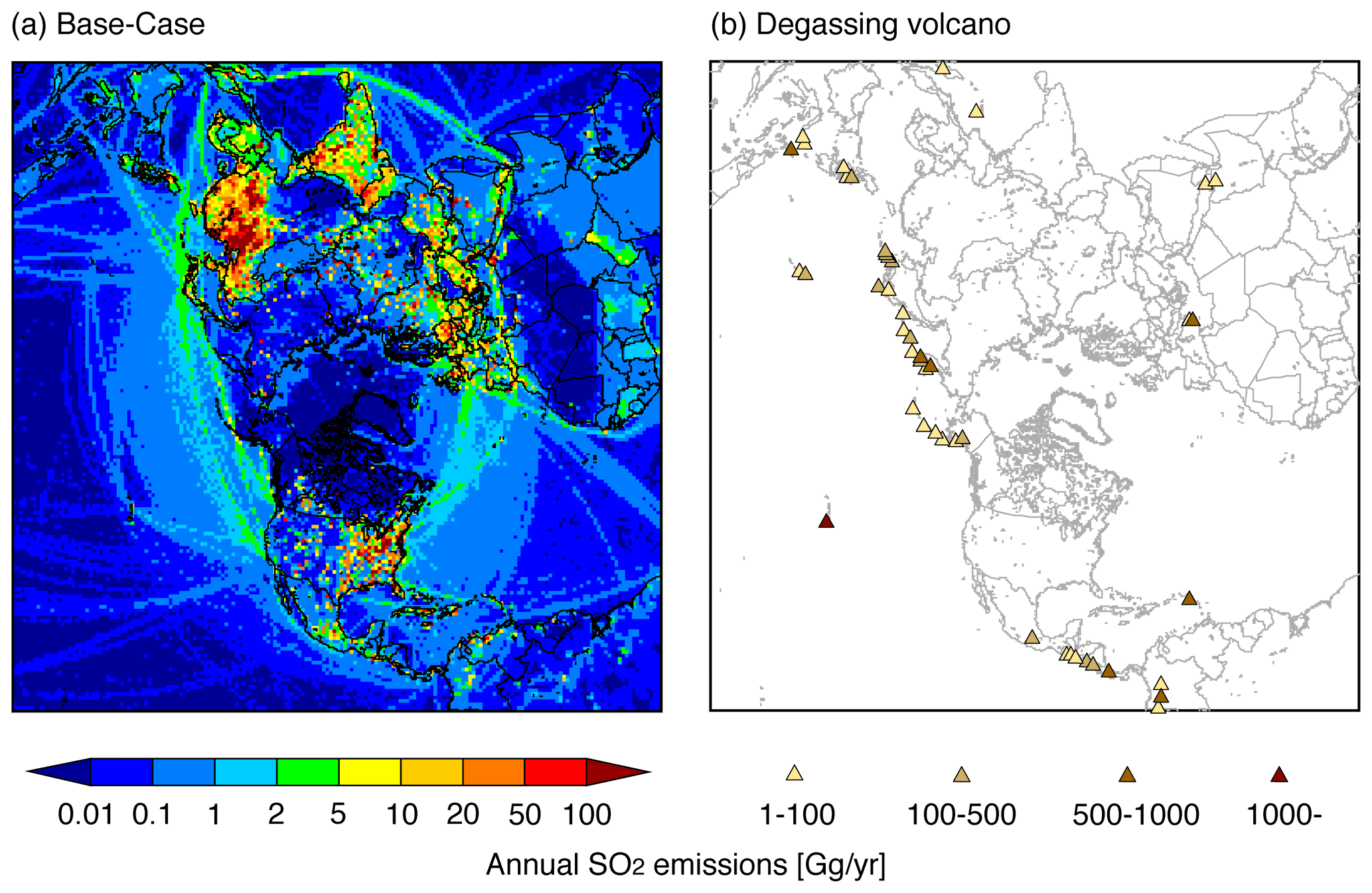
Figure 1 Geographical mapping of the (a) original SO₂ emissions used in H-CMAQ and (b) degassing volcanic annual SO₂ emissions incorporated in this study during 2010.

Earlier development and applications with the H-CMAQ modeling system have not considered volcanic SO₂ emissions. In this study, degassing volcanic SO₂ emissions as annual amount estimated by Carn et al. (2017) are incorporated into H-CMAQ. The estimated emission of SO₂ from the 50 volcanoes within our Northern Hemisphere modeling domain (Fig. 1b) is 12.7 Tg yr⁻¹. Considering the characteristics of degassing process from volcanoes and the lack of any other information to accurately specify its temporal variations, we use a constant SO₂ emission rate in H-CMAQ based on the annual SO₂ emission estimates by Carn et al. (2017). Table 1 provides detailed information on these 50 volcanoes including name, location (longitude and latitude), altitude (as above sea level (a.s.l.)), and SO₂ emission rate. Kilauea located in Hawaii is estimated to have the highest amount of degassing SO₂ emissions. Taking into account the characteristics of the degassing process, volcanic degassing SO₂ emissions were allocated into the model vertical layer corresponding to the volcano's altitude. This approach was also taken in another global model analysis (Chin et al., 1996; Ge et al., 2016). Even though in principle volcanic degassing emissions could be assigned to the first model layer because CMAQ uses a terrain-following vertical coordinate system, the 108 km grid spacing used in CMAQ does not allow the model to adequately resolve localized terrain peaks such as volcanoes, and assigning their emissions to the first model layer would not account for the fact that in reality these emissions typically occur above the mixed layer. Therefore, the vertical layer to which volcanic degassing emissions were assigned was determined by first calculating the difference between the altitude of a given volcano (Table 1) and the CMAQ terrain height for the cell in which it is located and then determining the vertical CMAQ layer corresponding to this difference. A schematic of the resultant assigned vertical layer is illustrated in Fig. 2. Most of volcanoes are located between altitudes of 500–5000 m a.s.l. (Table 1), and these correspond to layers 11–26 in the current model configuration.

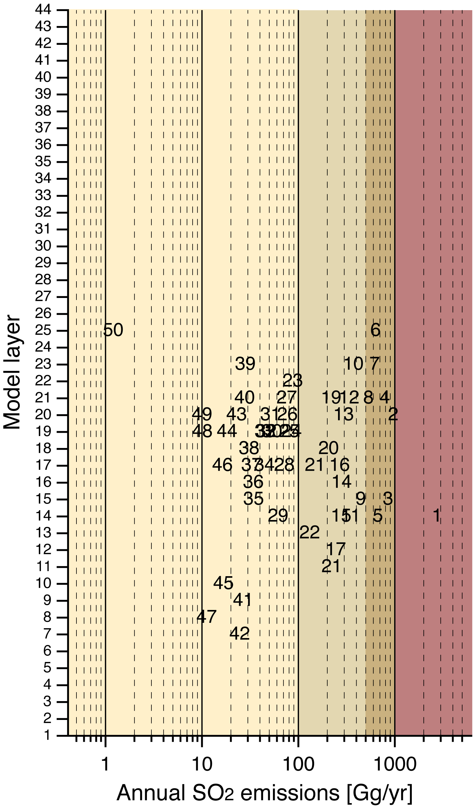
Figure 2 The model layers to which the SO₂ emissions from the 50 volcanoes considered in this study were assigned. See Table 1 for a listing of the volcanoes represented by each number in this figure. In Table 1, volcanoes are listed in decreasing order of their annual SO₂ emission amount.

Table 1 Information of volcanoes incorporated in this study.

2.2 Ground-based observations

As seen from Fig. 1b, the majority of the degassing volcanoes are located in the Pacific Rim region and their impacts on ${\mathrm{SO}}_{\mathrm{4}}^{\mathrm{2}-}$ levels in Japan have previously been studied (Itahashi et al., 2017a, b, 2019; Itahashi, 2018). To assess model performance in the Asian region, ground-based surface ${\mathrm{SO}}_{\mathrm{4}}^{\mathrm{2}-}$ observations were obtained from the Acid Deposition Monitoring Network in East Asia (EANET) program (EANET, 2020). During 2010, filter-pack measurements of ${\mathrm{SO}}_{\mathrm{4}}^{\mathrm{2}-}$ are available at 35 EANET sites with the following geographic distribution: 1 site in China, 3 sites in the South Korea, 12 sites in Japan, 2 sites in Mongolia, 4 sites in Russia, 5 sites in Thailand, 2 sites in Vietnam, 2 sites in the Philippines, 3 sites in Malaysia, and 1 site in Indonesia. Because the four-stage filter pack method in EANET measured total suspended particle, non-sea-salt (nss)-${\mathrm{SO}}_{\mathrm{4}}^{\mathrm{2}-}$ was calculated as $\text{nss-}{\mathrm{SO}}_{\mathrm{4}}^{\mathrm{2}-}={\mathrm{SO}}_{\mathrm{4}}^{\mathrm{2}-}-\mathrm{0.251}\times {\mathrm{Na}}^{+}$ in order to exclude the coarse-mode ${\mathrm{SO}}_{\mathrm{4}}^{\mathrm{2}-}$ produced with sea salt. For the simplicity, nss-${\mathrm{SO}}_{\mathrm{4}}^{\mathrm{2}-}$ for EANET observation is written as ${\mathrm{SO}}_{\mathrm{4}}^{\mathrm{2}-}$ throughout this article. Most of sites report two-week measurements, but some sites provide weekly or daily measurements. All available observation data were used in this study. As we have discussed in previous work (Itahashi et al., 2020a), Asian air pollution can impact on air quality over the USA; however, the magnitude of volcanic emissions on tropospheric ${\mathrm{SO}}_{\mathrm{4}}^{\mathrm{2}-}$ levels over North America has not been well studied. To evaluate the impact of volcanic SO₂ emissions located in the Northern Hemisphere on model performance, surface observations over the USA were obtained from the Clean Air Status and Trends Network (CASTNET), which covered remote and rural sites mostly over eastern USA (CASTNET, 2020), and the Integrated Monitoring of Protected Visual Environments (IMPROVE), which covered remote sites mostly over western USA (IMPROVE, 2020). Sampling frequency is weekly and daily (1 in every 3 days) for CASTNET and IMPROVE, respectively. A total of 84 CASTNET sites and 170 IMPROVE sites were available in 2010. Because of the coarse resolution of H-CMAQ simulations, measurements at urban sites were not considered in this study. To further examine the model's ability to represent the tropospheric sulfur distributions and budget, ambient SO₂ concentration at CASTNET sites and vertically integrated SO₂ column concentration measured by the OMI sensor were also analyzed. The OMI-measured SO₂ column was taken from the level-3 daily global sulfur dioxide product (OMSO2e) gridded into 0.25^∘ (Li et al., 2020). These gridded data were mapped to the H-CMAQ modeling domain and grid structure. This product contains the total column of SO₂ in the planetary boundary layer (PBL) with its center of mass altitude (CMA) at 0.9 km and lacked in the vertical sensitivity. Our previous study indicated that 1 km depth for CMA in the modeled SO₂ column yielded best comparisons with satellite-measured SO₂ column over East Asia (Itahashi et al., 2017b). The observed deficit grids by satellite were also considered in the analysis of modeled SO₂ column. The same approach to compare and evaluate SO₂ column was used in this study. Furthermore, ${\mathrm{SO}}_{\mathrm{4}}^{\mathrm{2}-}$ concentration in precipitation, precipitation amount, and ${\mathrm{SO}}_{\mathrm{4}}^{\mathrm{2}-}$ wet deposition were also evaluated relative to observations at EANET sites over Asia and the National Atmospheric Deposition Program's National Trends Network (NADP/NTN) over the USA (NADP, 2021). Measurements by wet-only sampler are available at 49 EANET sites with daily interval at most sites and weekly or 10 d interval at others sites (EANET, 2020). Observation of volume-weighted concentration in precipitation and total weekly wet deposition are available at 240 NADP sites.

To evaluate model performance with ground-based observations, the Pearson's correlation coefficient (R) with Student's t test is used for assessing the statistical significance level. The normalized mean bias (NMB) and the normalized mean error (NME) are also calculated as follows (e.g., Zhang et al., 2006; Itahashi et al., 2020b).

$$\begin{array}{}\text{(1)}& {\displaystyle }& {\displaystyle }R={\displaystyle \frac{{\sum }_{\mathrm{1}}^N\left(O_i-\stackrel{\mathrm{‾}}{O}\right)\left(M_i-\stackrel{\mathrm{‾}}{M}\right)}{\sqrt{{\sum }_{\mathrm{1}}^N{\left(O_i-\stackrel{\mathrm{‾}}{O}\right)}^{\mathrm{2}}}\sqrt{{\sum }_{\mathrm{1}}^N{\left(M_i-\stackrel{\mathrm{‾}}{M}\right)}^{\mathrm{2}}}}}\text{(2)}& {\displaystyle }& {\displaystyle }\text{NMB}={\displaystyle \frac{{\sum }_{\mathrm{1}}^N\left(M_i-O_i\right)}{{\sum }_{\mathrm{1}}^N{O}_i}}\text{(3)}& {\displaystyle }& {\displaystyle }\text{NME}={\displaystyle \frac{{\sum }_{\mathrm{1}}^N\left|M_i-O_i\right|}{{\sum }_{\mathrm{1}}^N{O}_i}},\end{array}$$

where N is the total observation number, O_i and M_i represent each individual observation and model result respectively, and $\stackrel{\mathrm{‾}}{O}$ and $\stackrel{\mathrm{‾}}{M}$ represent the arithmetical mean of observations and model results respectively. Based on a review of model performance over North America simulated by regional-scale air quality models, Emery et al. (2017) suggested threshold values of R>0.70, $\text{NMB}<\pm \mathrm{10}$ %, and NME<35 % as performance goal, and threshold values of R>0.40, $\pm \mathrm{10}\mathit{\%}<\text{NMB}<\pm \mathrm{30}$ %, and $\mathrm{35}\mathit{\%}<\text{NME}<\mathrm{50}$ % as performance criteria for daily ${\mathrm{SO}}_{\mathrm{4}}^{\mathrm{2}-}$.

3 Simulation results and discussion

3.1 Model evaluation

To provide an overview of the modeling results, we first present the annual-average ${\mathrm{SO}}_{\mathrm{4}}^{\mathrm{2}-}$ simulated by the base H-CMAQ configuration in Fig. 3a. High concentrations of ${\mathrm{SO}}_{\mathrm{4}}^{\mathrm{2}-}$ (greater than 5 µg m⁻³; red color in Fig. 3) are noted over East Asia, some parts of India, and the Arabian Peninsula corresponding to the intense SO₂ emissions shown in Fig. 1. The concentrations of ${\mathrm{SO}}_{\mathrm{4}}^{\mathrm{2}-}$ over Europe and USA were mostly 0.5–2.5 µg m⁻³ (blue color to green color in Fig. 3). The performance of this base case H-CMAQ simulation was evaluated over Asia and the USA through comparison with ${\mathrm{SO}}_{\mathrm{4}}^{\mathrm{2}-}$ measurements by EANET, CASTNET, and IMPROVE. The results of statistical analysis using R, NMB, and NME are listed in Table 2. Detailed maps of model results over Asia and the USA with overlaid distribution of surface observations are shown in Fig. 4. Figure 4 also contains a scatterplot between base H-CMAQ and surface observations; data for each month are shown using a different color. Significant scatter is noted in the correlation between the modeled and observed concentrations with an R of 0.43 over Asia (Table 2). Recent analysis of 12 regional models participating in the MICS-Asia model intercomparison study (Chen et al., 2019) however also revealed moderate correlations (0.46–0.79) with EANET observation. In terms of NMB and NME, NMB was −37.6 % and NME was 67.0 % in this study (Table 2). MICS-Asia showed NMB of −19.1 % as model ensemble mean but ranged from −67.0 % to +69.3 % for individual regional models (Chen et al., 2019). The H-CMAQ base case performance statistics were comparable or slightly worse compared to the previous regional-scale modeling studies (e.g., Itahashi, 2018; Itahashi et al., 2018; Yamaji et al., 2020; Chatani et al., 2020). This in part results from the inability of the coarse model grid resolution to resolve localized high-pollution episodes as seen in the scatterplot in Fig. 4. Over the USA, the spatial distribution patterns with low ${\mathrm{SO}}_{\mathrm{4}}^{\mathrm{2}-}$ in the western USA and comparatively higher values in the eastern USA are well captured in the base H-CMAQ simulation, though the model tended to underestimate across sites in the eastern USA. The observed annual averaged values by CASTNET were ranged between 2.5 and 3.4 µg m⁻³ over eastern USA. The scatterplot also verified the reasonable correspondence between model and observations. A winter minimum and summer maximum is noted both in the modeled and observed ${\mathrm{SO}}_{\mathrm{4}}^{\mathrm{2}-}$ values across the USA driven by expected variations in intensity of oxidant chemistry and conversion of S(IV) to S(VI). The statistical scores of R, NMB, and NME were within or close to the performance criteria proposed by Emery et al. (2017) over the USA and were also comparable to previous regional-scale modeling studies (e.g., Zhang et al., 2009, 2013). Overall, despite the use of coarse horizontal grid resolution of 108 km in H-CMAQ, model performance statistics were generally within the model performance statistics noted for other the regional modeling applications. One possible contributor to the noted ${\mathrm{SO}}_{\mathrm{4}}^{\mathrm{2}-}$ underestimation over Asian region in the base H-CMAQ could be from the missing of volcanic SO₂ emissions, especially in the Pacific Rim. Comparisons of model estimated SO₂ column distributions with satellite derived values are presented in Fig. S1 in the Supplement. The R value of 0.48 indicated the general agreement for the spatial distribution pattern of SO₂ column over the Northern Hemisphere with higher concentrations in regions with high anthropogenic SO₂ emissions (illustrated in Fig. 1); however, high SO₂ column over Hawaii evident in the satellite retrieval was not captured in the base H-CMAQ simulation due to the lack of volcanic SO₂ emissions. The impact of introducing the degassing volcanic SO₂ emissions is further discussed in the following sections.

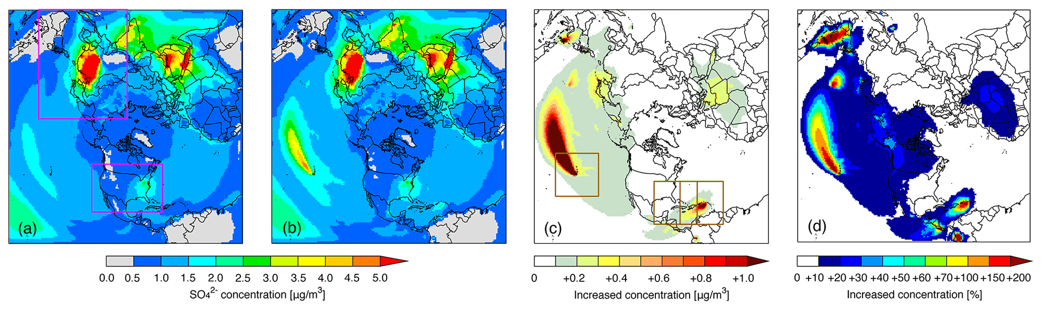
Figure 3 Simulated annual averaged ${\mathrm{SO}}_{\mathrm{4}}^{\mathrm{2}-}$ concentration in 2010 by (a) original H-CMAQ and (b) H-CMAQ with incorporation of volcanic SO₂ emissions, (c) increased concentration by the incorporation of volcanic SO₂ emissions, and (d) same as (c) but shown as relative percentages at the surface. The rectangular regions colored in pink in (a) indicate the Asia (top left) and USA (bottom right) subdomains used for detailed analysis. The rectangular regions colored in brown in (c) indicate areas for the analysis on specific site analysis that were largely impacted by degassing SO₂ volcanoes.

Table 2 Statistical analysis of modeled ${\mathrm{SO}}_{\mathrm{4}}^{\mathrm{2}-}$ concentration with observations.

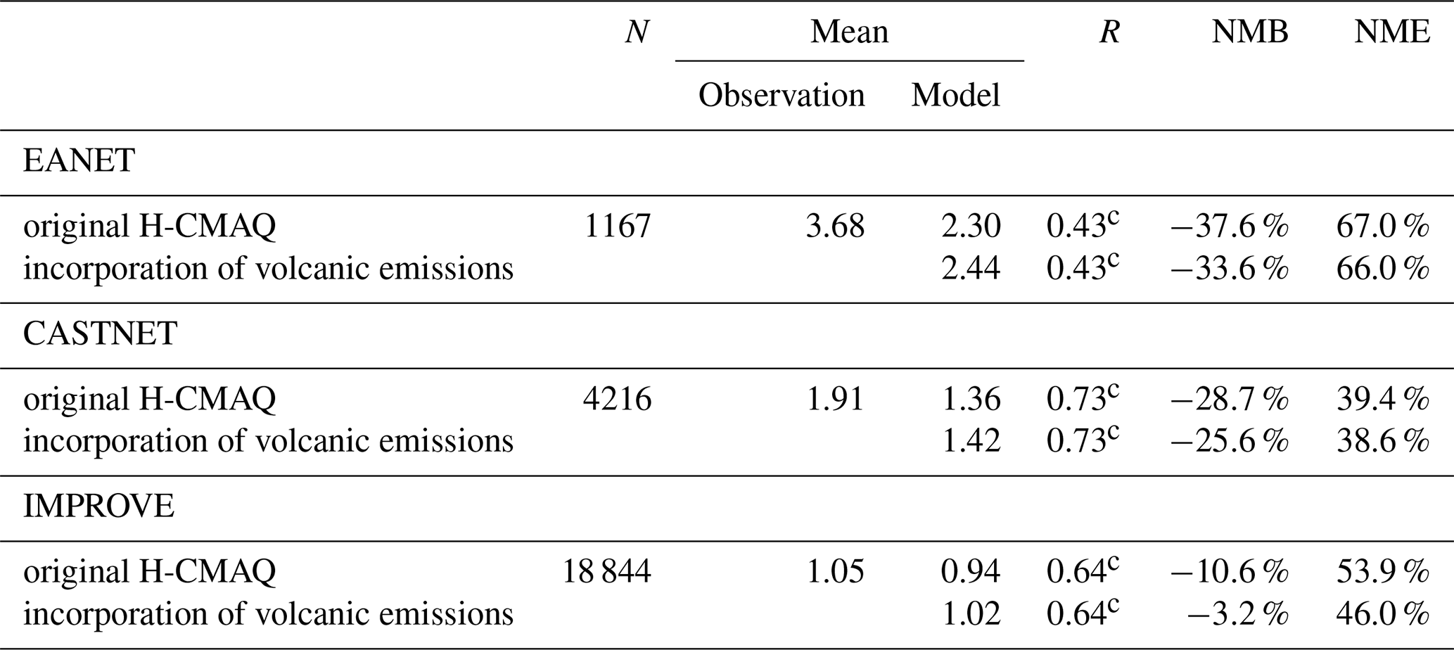
Note: The unit of mean for observations and simulations is µg m⁻³. Suggested threshold values of R>0.70, $\text{NMB}<\pm \mathrm{10}$ %, and NME<35 % as performance goal, and threshold values of R>0.40, $\pm \mathrm{10}\mathit{\%}<\text{NMB}<\pm \mathrm{30}$ %, and $\mathrm{35}\mathit{\%}<\text{NME}<\mathrm{50}$ % as performance criteria for daily ${\mathrm{SO}}_{\mathrm{4}}^{\mathrm{2}-}$ by the regional-scale modeling reviewed by Emery et al. (2017). Significance levels by Student's t test for correlation coefficients between observations and simulations are remarked as ^a p<0.05, ^b p<0.01, and ^c p<0.001, and lack of a mark indicates no significance.

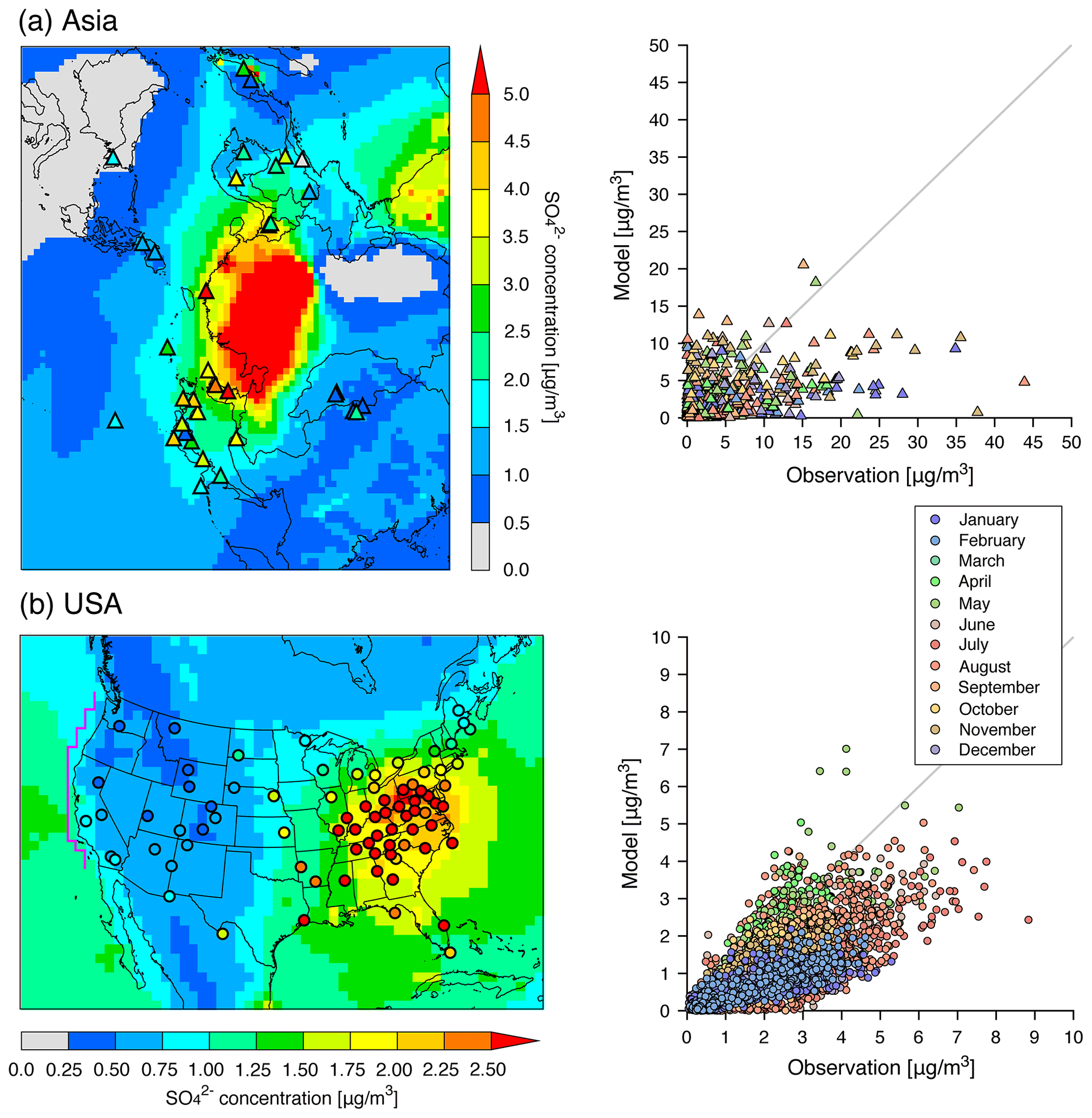
Figure 4 Simulated annual averaged ${\mathrm{SO}}_{\mathrm{4}}^{\mathrm{2}-}$ concentration in 2010 by original H-CMAQ over (a) Asia and (b) USA with overlaid EANET and CASTNET surface observations. Scatterplots between surface observation (EANET over Asia, and CASTNET over USA) and original H-CMAQ with identification colors for each month are also shown. Note that the color scale is different for Asia and USA. The pink line over the western USA in (b) is the defined as the western edge to analyze the vertical profile of ${\mathrm{SO}}_{\mathrm{4}}^{\mathrm{2}-}$ concentrations (see Fig. 7).

3.2 Impact of incorporating volcanic SO₂ emissions

The annual averaged ${\mathrm{SO}}_{\mathrm{4}}^{\mathrm{2}-}$ simulated after incorporating degassing volcanic SO₂ emission in H-CMAQ is shown in Fig. 3b, and the increase in concentrations relative to the base H-CMAQ is shown in Fig. 3c as absolute value and in Fig. 3d as the percentage change from the original H-CMAQ simulation. Impacts of including volcanic SO₂ emissions on tropospheric ${\mathrm{SO}}_{\mathrm{4}}^{\mathrm{2}-}$ are noted across the Pacific and up to the western coastline of the USA. It should be noted that even though the degassing volcanic emissions are allocated to upper model layers (see Fig. 2 and Table 1), they get transported through much of the troposphere with non-trivial impacts detected at the surface level. Increases of at least 0.1 µg m⁻³ in ${\mathrm{SO}}_{\mathrm{4}}^{\mathrm{2}-}$ concentration were simulated except over central Asia, equatorial and high-latitude regions, and the Atlantic Ocean, and most of the USA. The maximum increase of greater than 1.0 µg m⁻³ on an annual average basis was seen over the central Pacific (Fig. 3c). This increase is primarily attributed to SO₂ emission from Kilauea in Hawaii, which is estimated to have the highest degassing emissions (see Table 1). In addition, a moderate increase of up to 1.0 µg m⁻³ on an annual average basis was found over the Antilles islands in the Caribbean Sea. This was related to the volcanic activity of Soufrière Hills volcano located in Montserrat (no. 5 in strength; Table 1). Compared to the broad impacts found over Pacific Rim region, the impact of incorporating degassing volcanic SO₂ emission was limited over Europe and Africa. Increased concentrations ranging between 0.1–0.3 µg m⁻³ simulated over southern Europe and northern Africa region were caused by volcanoes in Italy (nos. 8 and 29 in Table 1), Ethiopia (no. 45 in Table 1), and Yemen (no. 47 in Table 1). Because only four degassing volcanoes in this region are considered in this study (see Fig. 1b), the impact itself was lower compared to other regions. In the terms of the percentage changes relative to the original H-CMAQ (depicted in Fig. 3d), increased concentration greater than 1.0 µg m⁻³ seen in Fig. 3c corresponded to +200 % change, and that of 0.1 µg m⁻³ corresponded to about a +10 % change. Over North America and the polar region, the increased absolute concentration was less than 0.1 µg m⁻³, whereas the percentage increase change was 10 %–30 %. For the annual average, it was found that the degassing volcanic SO₂ emissions increased ${\mathrm{SO}}_{\mathrm{4}}^{\mathrm{2}-}$ concentrations less than 0.1 µg m⁻³ over the entire USA, but this still represented a 10 %–20 % increase over the western USA.

The impacts on modeling performance by including volcanic SO₂ emissions are discussed based on the statistical analysis scores. In terms of the statistical analysis listed in Table 2, NMB and NME over Asia compared to EANET observation were improved, though the R values were not impacted significantly. This result was consistent with our previous findings that suggested volcanoes are an important source of tropospheric sulfur in East Asia (Itahashi et al., 2017a, b; Itahashi, 2018; Chatani et al., 2021). Over the USA, the base H-CMAQ had better modeling performance compared to Asia, and NMB and NME were improved when volcanic degassing emissions were included but R did not change. The improvements were noticeable in the comparison with observations at IMPROVE sites located in the western USA; NMB showed close agreement between H-CMAQ and IMPROVE observation. Both simulations of original H-CMAQ and H-CMAQ incorporating degassing SO₂ emissions showed model overestimation for ambient SO₂ concentration when compared to CASTNET observation as listed in Table S1 in the Supplement. The model performance statistics were comparable for the case incorporating degassing volcanic SO₂ emissions, indicating that additional SO₂ emissions from volcano were fully oxidized to ${\mathrm{SO}}_{\mathrm{4}}^{\mathrm{2}-}$ and thus have greater impact on changes in model performance for ${\mathrm{SO}}_{\mathrm{4}}^{\mathrm{2}-}$. The overestimation of SO₂ could be attributed to the insufficient oxidation process from SO₂ to ${\mathrm{SO}}_{\mathrm{4}}^{\mathrm{2}-}$ in the modeling system, because ${\mathrm{SO}}_{\mathrm{4}}^{\mathrm{2}-}$ values were still underestimated by incorporating volcanic SO₂ emissions. Coarse grid resolution leading to artificial dilution of SO₂ emissions could also contribute to overestimation of predicted ambient SO₂ levels relative to measurements at remote locations. The detailed discussion using conversion rate is further presented in next Sect. 3.3. The comparison of SO₂ column with satellite observation showed the improvement of R value from 0.48 to 0.56 due to improvements in representation of the spatial variability in tropospheric SO₂ distributions resulting from capturing the high SO₂ column in the vicinity of active volcanoes such as Kilauea as illustrated in Fig. S1. The evaluation for removal processes such as wet deposition is tabulated in Table S2 in the Supplement. The base H-CMAQ simulation tended to underestimate both ${\mathrm{SO}}_{\mathrm{4}}^{\mathrm{2}-}$ concentration in precipitation and wet deposition. The inclusion of volcanic SO₂ emission sources led to slight improvements in the NMB and R, but the NME was largely unaltered. From these evaluations, it is concluded that the incorporation of degassing volcanic SO₂ emissions helps to improve performance of simulated ${\mathrm{SO}}_{\mathrm{4}}^{\mathrm{2}-}$ in H-CMAQ by a small margin.

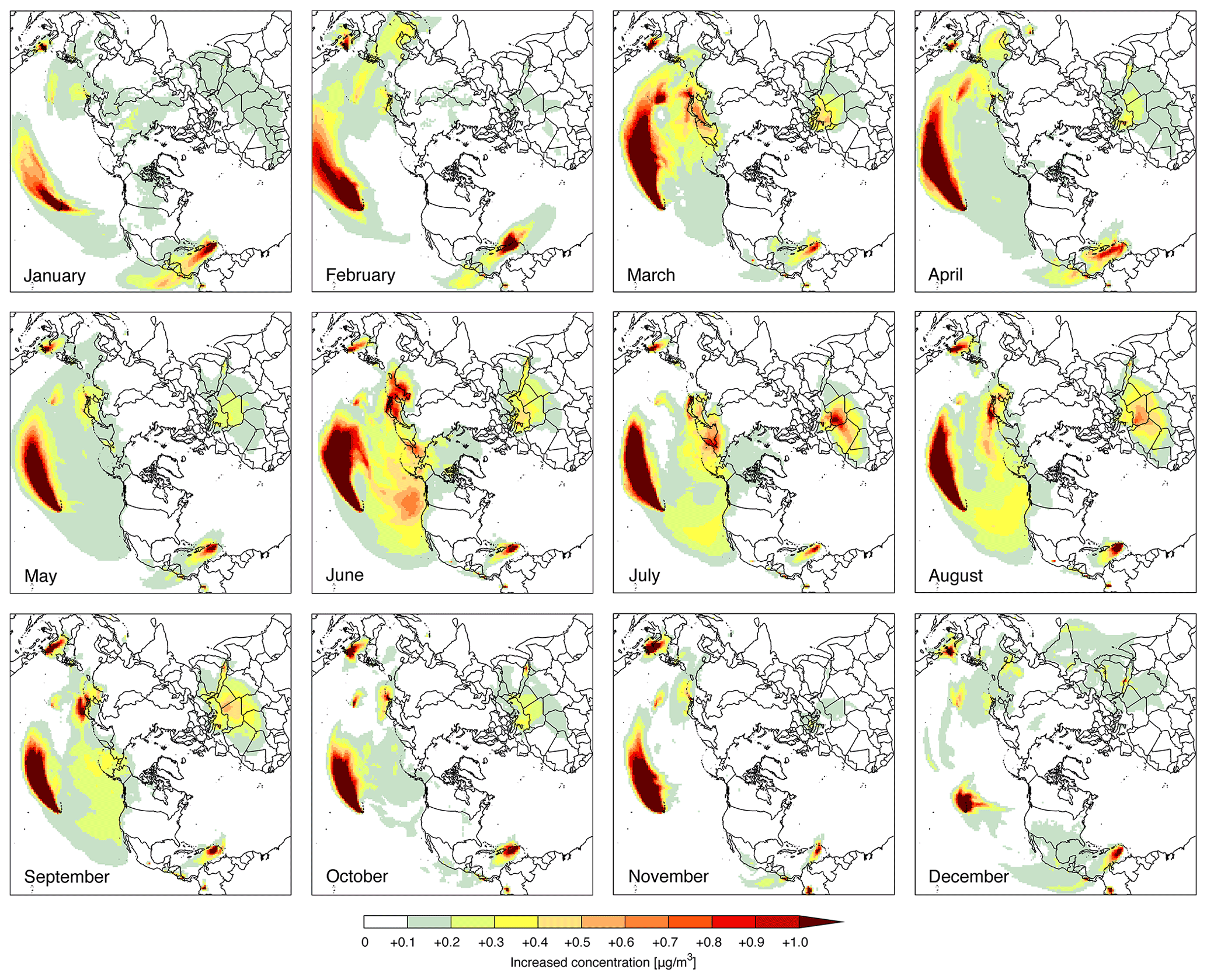
Figure 5 Simulated increased surface ${\mathrm{SO}}_{\mathrm{4}}^{\mathrm{2}-}$ concentration by the incorporation of volcanic SO₂ emissions over each month in 2010 at surface.

The impacts of degassing volcanic SO₂ emissions on seasonal ${\mathrm{SO}}_{\mathrm{4}}^{\mathrm{2}-}$ distributions and long-range transport were further analyzed by examining monthly mean contributions as illustrated in Fig. 5. Similar to the annual mean distributions shown in Fig. 3c, the maximum impact was seen over the central Pacific associated with emissions from the Kilauea volcano throughout the year. Regarding its monthly variation, the increased concentrations at the surface level during spring to summer season (from April to September) were higher than those during winter (especially, December and January). The higher impacts during summer result both from higher rates of SO₂ to ${\mathrm{SO}}_{\mathrm{4}}^{\mathrm{2}-}$ conversion as well as enhanced convective mixing. In contrast during winter lower conversion rates and a more stably stratified atmosphere result in reduced ${\mathrm{SO}}_{\mathrm{4}}^{\mathrm{2}-}$ from volcanic emissions at the surface. The enhanced ${\mathrm{SO}}_{\mathrm{4}}^{\mathrm{2}-}$ associated with emissions from the Kilauea volcano (with highest emission rate as indicted in Table 1) stretches across the central Pacific to the western shores of the USA, with enhancements in surface-level ${\mathrm{SO}}_{\mathrm{4}}^{\mathrm{2}-}$ on a monthly-mean basis greater than 0.1 µg m⁻³ across portions of the western USA. The contributions of volcanoes located on the Kamchatka Peninsula (nos. 2, 6, 12, 14, 16, 19, and others in Table 1) are estimated to be comparatively lower on an annual average basis but may be higher episodically under conducive transport condition. During the winter season, the impacts from Kilauea did not reach the western USA; however, the impacts from Soufrière Hills located in Montserrat (no. 5 in Table 1) reached the southern USA. Further analysis focused on specific sites is discussed in next section.

3.3 Impacts of volcanic SO₂ emissions at specific sites

Detailed analysis at an observation site located in Hawaii was further conducted to evaluate model performance. According to the observation summary (WRAP, 2020), a large fraction of the measured ${\mathrm{SO}}_{\mathrm{4}}^{\mathrm{2}-}$ at this location is attributed to SO₂ emissions associated with volcanic activity from Kilauea. A total of three IMPROVE sites are located in the state of Hawaii. One of the sites is located in the Hawaii Volcanoes National Park and is in the vicinity of the Kilauea volcano (site name is HAVO1). Comparison of model and observed temporal variation in ${\mathrm{SO}}_{\mathrm{4}}^{\mathrm{2}-}$ at this site is displayed in Fig. 6a. The observation showed higher concentration during the winter season, and the average concentration through 2010 was 2.37 µg m⁻³. The base H-CMAQ simulation showed largely invariant concentrations throughout the year with an annual average value of 0.87 µg m⁻³ and a negative correlation against observation. The statistical scores of NMB showed high negative bias because the base H-CMAQ did not capture the higher concentration observed during winter. By including the degassing volcano emissions, the model showed spikes for higher concentration days. Though the observed maximum peak of 30 µg m⁻³ on 3 January was not fully captured, the simulated values of around 10 µg m⁻³ by incorporating the volcano emissions were significantly enhanced relative to the base model. The result showed that the averaged concentration was 2.87 µg m⁻³, and NMB showed +21.2 % with moderate correlation by R of 0.36. The inclusion of degassing volcanoes led to better performance at this specific site; however, the deterioration in the value of NME should be considered. While the H-CMAQ simulations with incorporated volcanoes also showed lower ${\mathrm{SO}}_{\mathrm{4}}^{\mathrm{2}-}$ concentrations during summer season compared to winter, the simulated summertime values were higher than observed and led to a persistent positive bias during this season. A potential reason for this behavior could be the treatment of degassing volcanoes SO₂ emissions as a constant flux in this study. For example, a case study targeted to quantify the air quality impacts of the Kilauea eruption in 2018 showed the importance of temporal variation of emissions and plume rise calculation (Tang et al., 2020). Our results indicate general improvements of model performance by including degassing volcano emissions represented by a constant temporal and vertical profile, but refining the treatment of these aspects should be studied in future work. In terms of SO₂ concentration, IMPROVE sites do not measure it. Based on an intensive observational study at Kilauea during January and February 2013, SO₂ concentrations showed large variations from below 1 ppbv under conditions of no influence of the volcanic plume to over 3000 ppbv when air masses influenced by the volcanic plume were sampled (Kroll et al., 2015). In the base H-CMAQ calculation, the daily averaged SO₂ mixing ratios for the grid cell with the Kilauea volcano ranged from below 0.01 to 0.14 ppbv, while the annual mean value was 0.03 ppbv. In contrast, when volcanic emissions were incorporated in H-CMAQ, simulated SO₂ mixing ratios ranged from below 0.03 to 1088.20 ppbv with an annual mean value of 221.08 ppbv, which better matches the dynamic range inferred from the SO₂ measurements in the vicinity of the Kilauea volcano reported in Kroll et al. (2015).

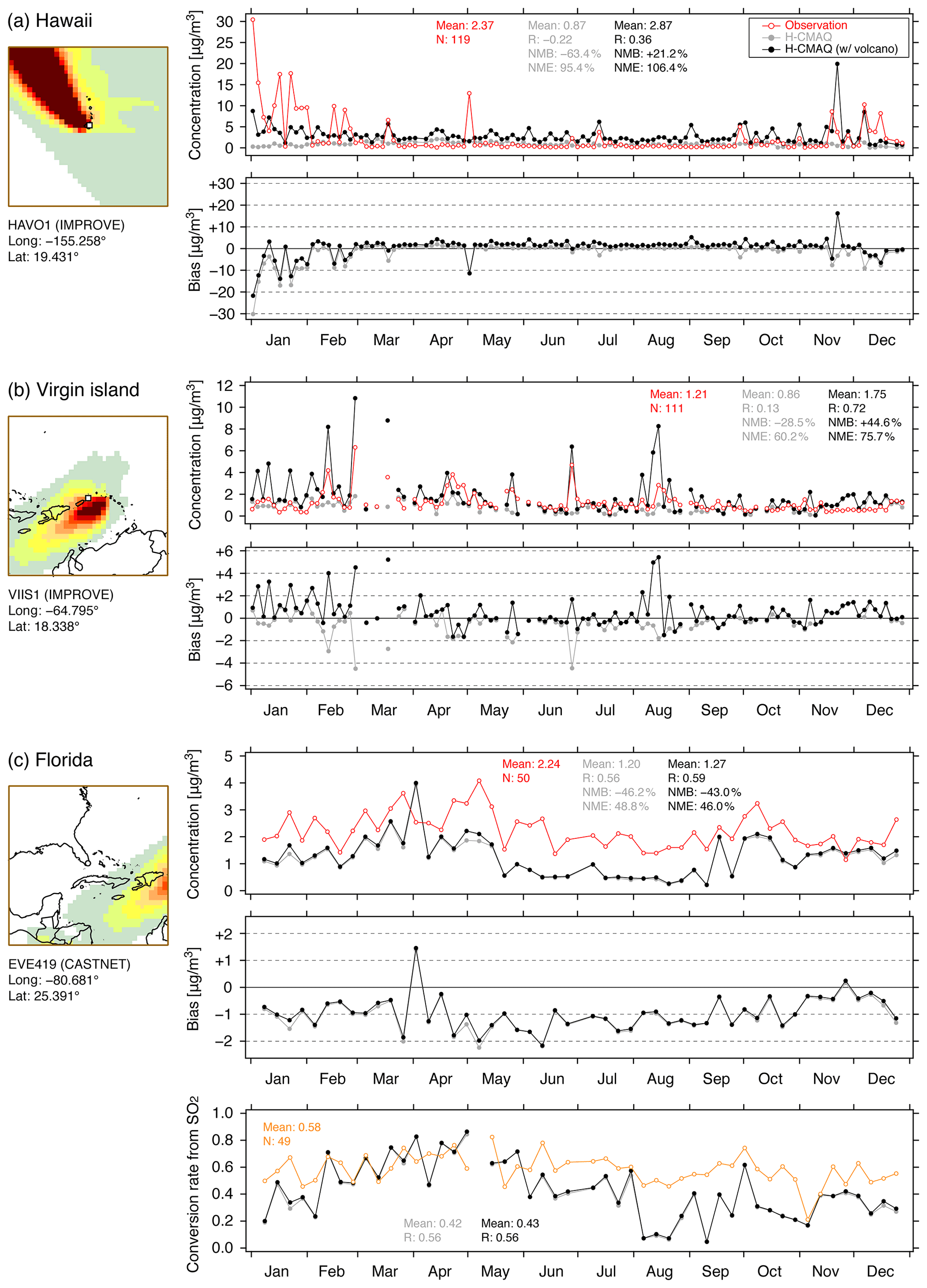
Figure 6 Temporal variation of observed and simulated ${\mathrm{SO}}_{\mathrm{4}}^{\mathrm{2}-}$ concentrations and simulation biases at (a) Hawaii IMPROVE site (HAVO1), (b) Virgin Islands IMPROVE site (VIIS1), and (c) Florida CASTNET site (EVE419) in 2010. Red open circle denotes observations, and gray and black closed circles denote original H-CMAQ and H-CMAQ incorporating volcanoes, respectively. Statistical scores are indicated in the inset. The comparison of conversion rate from SO₂ to ${\mathrm{SO}}_{\mathrm{4}}^{\mathrm{2}-}$ is also shown in (c).

A second location-specific analysis was conducted at a site located in the Virgin Islands and in the state of Florida. As seen in the monthly-average spatial distribution patterns (Fig. 5), the influence of volcanic activity of Soufrière Hills located in Montserrat is more prominent during winter. The nearest observation site from Soufrière Hills is the IMPROVE site VIIS1, and the southernmost measurement location in Florida (see Fig. 4) is the CASTNET site EVE419 and comparison of modeled values with observations at these locations is shown in Fig. 6b and c. At VIIS1 (Fig. 6b), the base H-CMAQ simulation showed invariant concentrations throughout the year with an annual average value of 0.86 µg m⁻³. The statistical scores of R showed scattered correspondence between model and observation; NMB showed negative bias because the base H-CMAQ did not capture the episodical peak concentration. By including the degassing volcanic SO₂ emissions, the model caught episodical peak events. The statistical scores showed that the averaged concentration was 1.75 µg m⁻³, and NMB showed +44.6 %, and R was dramatically improved to 0.72. The deterioration in the value of NME was found because of the continuous model overestimation. As also suggested for the case in Hawaii, further refinement on emission treatments is required. At EVE419 (Fig. 6c), the seasonal pattern with summer minima was captured by H-CMAQ but underestimated throughout the year. Increased concentrations through the incorporation of volcanic emissions are noted during January, late April to early May, and December. The increase during late April to early May was not seen from the monthly averaged spatial distribution (Fig. 5); hence these could be the episodic long-range transport by southeasterly winds. Because of these increased concentrations, all statistical scores of R, NMB and NME showed improvement compared to the base H-CMAQ. CASTNET also provides measurements of weekly-average SO₂ mixing ratios, which are used to evaluate the model's performance for SO₂ prediction, as shown in Table S1. In addition to domain-mean evaluation, we evaluated SO₂ at the EVE419 site in Florida. At this site, the observed annual mean was 0.61 ppbv, whereas base H-CMAQ and H-CMAQ with volcanic SO₂ emissions both showed 0.77 ppbv. Additionally, the results suggest that the SO₂ from volcanic sources was fully oxidized to ${\mathrm{SO}}_{\mathrm{4}}^{\mathrm{2}-}$ during long-range transport, and there was no direct transport of SO₂ itself at this site. At this CASTNET site of EVE419 at Florida, the conversion rate from SO₂ to ${\mathrm{SO}}_{\mathrm{4}}^{\mathrm{2}-}$ was further examined. This conversion rate is defined as ${\mathrm{SO}}_{\mathrm{4}}^{\mathrm{2}-}/({\mathrm{SO}}_{\mathrm{4}}^{\mathrm{2}-}+{\mathrm{SO}}_{\mathrm{2}})$, and a higher value indicates the oxidation from SO₂ to ${\mathrm{SO}}_{\mathrm{4}}^{\mathrm{2}-}$. The temporal variation of conversion rate is also plotted in Fig. 6b. The conversion rate was lower in the cold season and higher in the warm season, and this general feature was captured by model. The mean of conversion rate throughout the year was 0.58 in the observation, whereas original H-CMAQ was 0.42. By incorporating degassing volcanic SO₂ emissions, the mean of conversion rate increased in 0.43 but still underestimated the observed value. Since data from routine measurement networks are not designed to specifically characterize impacts of volcanic emissions on atmospheric sulfur budgets, these observations are unable to unambiguously quantify any modulation in S(IV) to S(VI) conversion rates due to the presence of volcanic emissions as also evidenced by the small change in the estimated conversion rate between the simulations with and without volcanic degassing emissions. Collectively, these results and those summarized in Table 2 and Fig. 4 suggest that inclusion of degassing volcanic emissions moderately improves model performance statistics for simulated ${\mathrm{SO}}_{\mathrm{4}}^{\mathrm{2}-}$ spatial distributions and temporal variations. Note that the incorporation of volcanic degassing emissions does not necessarily improve model performance in all instances due to the presence of uncertainties and potentially compensating errors in other parts of the modeling system (i.e., model input fields like other emissions and meteorology, model representation of processes such as chemical reactions and deposition) and suitability of the measurement network (e.g., proximity) in characterizing the variability in tropospheric composition due to volcanic degassing emissions. Nonetheless, incorporating the degassing volcanic SO₂ emissions which clearly occur in nature is an important aspect for enhancing the completeness of the modeling system itself. Quantifying the space and time variations of persistent volcanic degassing emissions on tropospheric composition is important, especially in the context of using models to characterize background pollution levels and anthropogenic enhancements of tropospheric pollutants and associated health and visibility impacts.

3.4 Impact on upper troposphere

Finally, the impacts caused by including the degassing volcanoes were investigated throughout the troposphere. In a subsequent analysis, the boundary layer is defined from the surface to 750 hPa, and the free troposphere is defined from 750 to 250 hPa, and pressure levels of 750, 500, and 250 hPa are used to refer to the bottom, middle, and top of the free troposphere similar to our previous study (Itahashi et al., 2020a). The vertical profile of simulated ${\mathrm{SO}}_{\mathrm{4}}^{\mathrm{2}-}$ concentration averaged along the edge of western USA (defined in Fig. 4b) was analyzed. The vertical profile of the base H-CMAQ and the increased concentration due to incorporating the degassing volcanic SO₂ emission are plotted in Fig. 7. Modeled ${\mathrm{SO}}_{\mathrm{4}}^{\mathrm{2}-}$ concentrations decreased from the surface to upper layers, and concentration levels were greater in summer than those during winter (e.g., Fig. 4 for surface results). Incorporation of volcanic SO₂ emissions increased monthly mean ${\mathrm{SO}}_{\mathrm{4}}^{\mathrm{2}-}$ within the boundary layer by up to 0.4 µg m⁻³ during June to September. This increase is consistent with the spatial distribution at surface depicted in Fig. 5, but it also occurs through the depth of the boundary layer. During other months, the simulated concentration increases were less than 0.1 µg m⁻³ throughout the free troposphere.

Figure 7 Vertical profile of simulated ${\mathrm{SO}}_{\mathrm{4}}^{\mathrm{2}-}$ concentration of each month in 2010 at the edge of western USA (see Fig. 4): (a) original H-CMAQ and (b) increased concentration by the incorporation of volcanic SO₂ emissions.

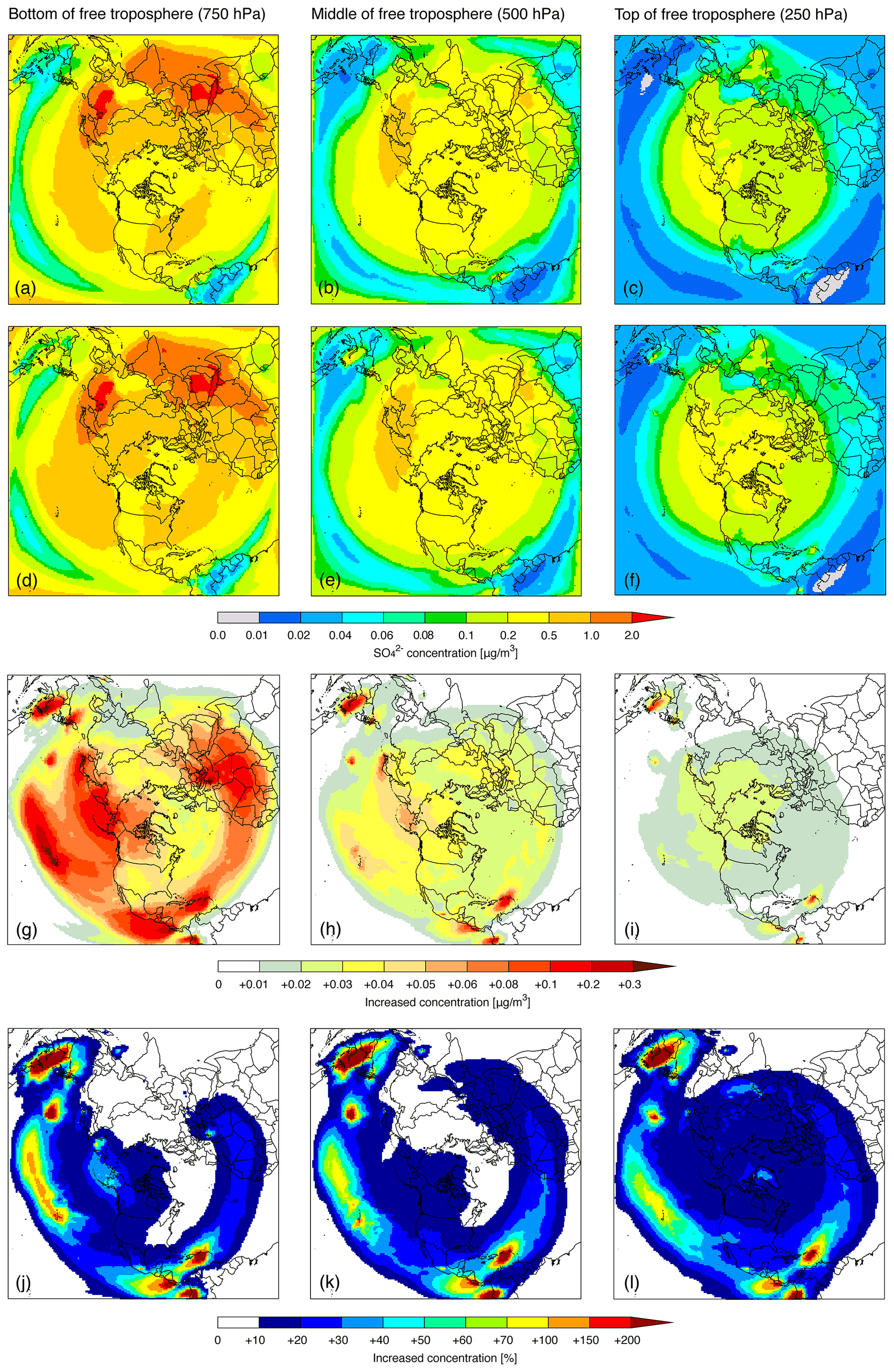
Figure 8 Simulated annual averaged ${\mathrm{SO}}_{\mathrm{4}}^{\mathrm{2}-}$ concentration in 2010 by (a–c) original H-CMAQ and (d–f) H-CMAQ with incorporation of volcanic SO₂ emissions, (g–i) increased concentration by the incorporation of volcanic SO₂ emissions, and (j–l) same as (g–i) but shown as relative percentage at the bottom of the free troposphere (750 hPa; a, d, g, j), middle of the free troposphere (500 hPa; b, e, h, k), and top of the free troposphere (250 hPa; c, f, i, l).

Simulated annual average ${\mathrm{SO}}_{\mathrm{4}}^{\mathrm{2}-}$ concentration distributions at the bottom, middle, and top of the free troposphere from the two model simulations and the estimated increase due to incorporation of degassing volcanic emissions are shown in Fig. 8. The simulated spatial distribution of ${\mathrm{SO}}_{\mathrm{4}}^{\mathrm{2}-}$ exhibited similar patterns at the bottom of the free troposphere (Fig. 8a and d) with higher concentration over Asian region. However, significant differences in the magnitude and spatial distributions of simulated ${\mathrm{SO}}_{\mathrm{4}}^{\mathrm{2}-}$ between the two simulations are noted at the middle and top of the free troposphere as seen from higher concentration in the North Pacific region close to the North Pole (Fig. 8b, c, e, and f). The maximum concentrations at the top of the free troposphere (Fig. 8c and f) decreased by a factor of 10 compared to those at the surface (Fig. 3a and b). The increased concentration by including degassing volcanoes showed the increment corresponded to the location of volcanoes. In contrast to the increased concentrations over the Pacific Rim region found at the surface level (Fig. 3c), increased ${\mathrm{SO}}_{\mathrm{4}}^{\mathrm{2}-}$ over the Bering Sea was noticeable at the bottom of the free troposphere (Fig. 8g). Over this area, increased ${\mathrm{SO}}_{\mathrm{4}}^{\mathrm{2}-}$ values ranging from +0.08 to +0.2 at the bottom of free troposphere were found. This is mainly caused by the Mutnovsky, Gorely, Kliuchevskoi (Klyuchevskoi), and Bezymianny volcanoes (nos. 5 and 6 in Table 1), other volcanoes located on the Kamchatka Peninsula (nos. 12, 14, 16, 19, 24, 35, 36, and 48), and volcanoes over the Alaska Peninsula (nos. 37–40, and 46) in the surrounding Bering Sea. These volcanoes were characterized by the relatively higher altitude (no. 6 was allocated into the highest altitude) considered in this study (Table 1 and Fig. 2). The increased concentrations at the middle and top of the free troposphere were widely distributed with centering on the North Pole. These increased concentrations indicated that while volcanic emissions were assumed to be injected into the lower and middle free troposphere (Fig. 2), their impacts on secondary ${\mathrm{SO}}_{\mathrm{4}}^{\mathrm{2}-}$ production were detected throughout the free troposphere. Based on the percentage change relative to the original H-CMAQ simulation, Fig. 8 further shows that the spatial extent of the impact of including degassing volcanic SO₂ emissions on ${\mathrm{SO}}_{\mathrm{4}}^{\mathrm{2}-}$ increased with height, with most of the Northern Hemisphere showing increases exceeding 10 % at 250 hPa.

4 Conclusions

Previous work on the development and evaluation of the H-CMAQ model has historically not considered volcanic SO₂ emissions. In this study, satellite-constrained SO₂ emissions from 50 degassing volcanoes over the Northern Hemisphere are incorporated into H-CMAQ, and their impacts on tropospheric ${\mathrm{SO}}_{\mathrm{4}}^{\mathrm{2}-}$ are evaluated for model simulations of the calendar year 2010. Model performance was evaluated using network observations of EANET over Asia and CASTNET and IMPROVE over the USA. The base H-CMAQ underestimated ${\mathrm{SO}}_{\mathrm{4}}^{\mathrm{2}-}$, and this was partially rectified by incorporating volcanic SO₂ emissions as indicated through improvements in the statistical scores of R, NMB, and NME. Over Asia, the largest increases in ${\mathrm{SO}}_{\mathrm{4}}^{\mathrm{2}-}$ were simulated in the vicinity of the volcanoes, especially over Japan and Indonesia. Over the USA, the largest impact over the central Pacific was caused by including the Kilauea volcano, and its impacts on the continental USA were limited to the western USA during the summer. The emissions from the Soufriére Hills volcano located in Montserrat affected the southern USA during the winter season. Analysis of temporal variations at measurement sites located in Hawaii, the Virgin Islands, and Florida showed improvements in modeling performance as a result of the inclusion of volcanic SO₂ emissions. The changes in simulated aloft ${\mathrm{SO}}_{\mathrm{4}}^{\mathrm{2}-}$ concentration were investigated, and it was revealed that the impacts were detected up to the top of the free troposphere, although the considered SO₂ emissions were injected in the lower and middle of the free troposphere.

The results suggest that emission of SO₂ resulting from volcanic degassing is one of the important sources that should be considered in the modeling system as it regulates tropospheric ${\mathrm{SO}}_{\mathrm{4}}^{\mathrm{2}-}$ levels not only in the vicinity of the volcano but also through long-range transport that modulates background levels at downwind continents. In addition to inclusion of persistent degassing emissions, eruptive volcanic emissions can also play an important role in episodically modulating tropospheric sulfur budgets and radiative forcing (Schmidt et al., 2012, 2018). As seen from the analysis of model and measured values at the Kilauea volcanic site in this study, the approach to treat the degassing volcanic SO₂ emissions as assigned in one model vertical layer without any temporal variation sometimes leads to the unexpected positive bias on cleaner days. A more realistic treatment of temporal variation of degassing gases and the related meteorological parameters (e.g., local wind speed) would be useful to further refine the modeling performance of ${\mathrm{SO}}_{\mathrm{4}}^{\mathrm{2}-}$ produced via volcanic SO₂ emission.