EC-Earth3-AerChem: a global climate model with interactive aerosols and atmospheric chemistry participating in CMIP6

This paper documents the global climate model EC-Earth3-AerChem, one of the members of the EC-Earth3 family of models participating in the Coupled Model Intercomparison Project Phase 6 (CMIP6). EC-Earth3-AerChem has interactive aerosols and atmospheric chemistry and contributes to the Aerosols and Chemistry Model Intercomparison Project (AerChemMIP). In this paper, we give an overview of the model, describe in detail how it differs from the other EC-Earth3 configurations, and outline the new features compared with the previously documented version of the model (EC-Earth 2.4). We explain how the model was tuned and spun up under preindustrial conditions and characterize the model's general performance on the basis of a selection of coupled simulations conducted for CMIP6. The net energy imbalance at the top of the atmosphere in the preindustrial control simulation is on average −0.09 W m⁻² with a standard deviation due to interannual variability of 0.25 W m⁻², showing no significant drift. The global surface air temperature in the simulation is on average 14.08 ^∘C with an interannual standard deviation of 0.17 ^∘C, exhibiting a small drift of 0.015 ± 0.005 ^∘C per century. The model's effective equilibrium climate sensitivity is estimated at 3.9 ^∘C, and its transient climate response is estimated at 2.1 ^∘C. The CMIP6 historical simulation displays spurious interdecadal variability in Northern Hemisphere temperatures, resulting in a large spread across ensemble members and a tendency to underestimate observed annual surface temperature anomalies from the early 20th century onwards. The observed warming of the Southern Hemisphere is well reproduced by the model. Compared with the ECMWF (European Centre for Medium-Range Weather Forecasts) Reanalysis version 5 (ERA5), the surface air temperature climatology for 1995–2014 has an average bias of −0.86 ± 0.05 ^∘C with a standard deviation across ensemble members of 0.35 ^∘C in the Northern Hemisphere and 1.29 ± 0.02 ^∘C with a corresponding standard deviation of 0.05 ^∘C in the Southern Hemisphere. The Southern Hemisphere warm bias is largely caused by errors in shortwave cloud radiative effects over the Southern Ocean, a deficiency of many climate models. Changes in the emissions of near-term climate forcers (NTCFs) have significant effects on the global climate from the second half of the 20th century onwards. For the SSP3-7.0 Shared Socioeconomic Pathway, the model gives a global warming at the end of the 21st century (2091–2100) of 4.9 ^∘C above the preindustrial mean. A 0.5 ^∘C stronger warming is obtained for the AerChemMIP scenario with reduced emissions of NTCFs. With concurrent reductions of future methane concentrations, the warming is projected to be reduced by 0.5 ^∘C.

1 Introduction

EC-Earth is a global climate and Earth system model developed by a European consortium of meteorological services, research institutes, and high-performance computing centers (Hazeleger et al., 2010, 2012). Activities in recent years have been dedicated to the development of the third generation of the model and participation in the Coupled Model Intercomparison Project Phase 6 (CMIP6; Eyring et al., 2016). The basic CMIP6 configuration of the model (EC-Earth version 3.3.1.1, hereafter referred to as EC-Earth3) consists of an atmospheric general circulation model (GCM) based on cycle 36r4 of the Integrated Forecasting System (IFS) from the European Centre for Medium-Range Weather Forecasts (ECMWF), coupled to the NEMO-LIM3 global ocean–sea-ice model from the Nucleus for European Modelling of the Ocean (NEMO) release 3.6 (Rousset et al., 2015). Other CMIP6 configurations of EC-Earth include additional modules for simulating dynamic vegetation, the carbon cycle, aerosols and atmospheric chemistry, or the Greenland ice sheet. Low- and high-resolution configurations have also been developed. An overview of the different configurations is given by Döscher et al. (2021). Specific model configurations will be documented in separate publications. This paper documents the configuration with interactive aerosols and atmospheric chemistry (EC-Earth-AerChem version 3.3.3, hereafter EC-Earth3-AerChem). It is with this configuration that the EC-Earth consortium participates in the Aerosols and Chemistry Model Intercomparison Project (AerChemMIP; Collins et al., 2017).

The distinguishing feature of EC-Earth3-AerChem, compared with the other EC-Earth configurations applied in CMIP6, is that it simulates tropospheric aerosols and the reactive greenhouse gases methane and ozone. In all other configurations these are prescribed as described by Döscher et al. (2021). Although methane and stratospheric ozone are not fully prescribed in EC-Earth3-AerChem as in the other configurations, they are constrained by the CMIP6 forcing data sets of Meinshausen et al. (2017, 2020) and Checa-Garcia et al. (2018), respectively. As a result, the main differences between EC-Earth3-AerChem and the other CMIP6 configurations of EC-Earth are related to tropospheric aerosols and tropospheric and lower-stratospheric ozone as well as how they interact with the climate system.

In this paper, we describe the model and present the first results from CMIP6 simulations. The remainder of the paper is structured as follows: Sect. 2 provides a description of the model. It gives an outline of the main general model characteristics, and documents the treatment of aerosols and their interactions with radiation and clouds; atmospheric chemistry and chemical boundary conditions; anthropogenic and natural emissions; and, finally, some relevant technical and numerical aspects of the model. The applied tuning and spin-up procedures are outlined in Sect. 3. Results from CMIP6 simulations are presented in Sect. 4. The analysis presented in Sect. 4 focuses on the effective equilibrium climate sensitivity and the transient climate response, the net energy imbalance in the simulations, and the long-term evolution and present-day climatology of surface air temperatures. Finally, we end the paper with a discussion and conclusions in Sect. 5.

2 Model description

2.1 General

EC-Earth3-AerChem is essentially EC-Earth3 (Döscher et al., 2021) extended with an additional component to simulate aerosols and atmospheric chemistry. The atmospheric GCM is based on IFS cycle 36r4, which includes the land surface model H-TESSEL (revised hydrology version of TESSEL, the Tiled ECMWF Scheme for Surface Exchanges over Land; Balsamo et al., 2009). The horizontal resolution of the GCM is T_L255 (triangular truncation at wavenumber 255 in spectral space with a linear N128 reduced Gaussian grid, corresponding to a spacing of about 80 km). The atmospheric grid consists of 91 layers in the vertical direction and has a model top at 0.01 hPa. Following ECMWF recommendations, the model time step for this resolution is set to 45 min.

The McRad radiation package of cycle 36r4 consists of a shortwave (SW) and longwave (LW) radiation scheme based on the Rapid Radiative Transfer Model for General Circulation Models (RRTMG), and it uses the Monte Carlo independent column approximation (McICA) to treat the radiative transfer in clouds (Morcrette et al., 2008). Clouds and large-scale precipitation are described by prognostic equations for cloud liquid water, cloud ice, rain, snow, and a grid box fractional cloud cover.

Compared with the original model from IFS cycle 36r4, several adjustments and updates have been made in EC-Earth (Döscher et al., 2021). These include the application of global mass fixers for dry air and humidity (Diamantakis and Flemming, 2014), a resolution-dependent parameterization of non-orographic gravity wave drag (Davini et al., 2017), and a diagnostic convective closure, which is dependent on the convective available potential energy (Bechtold et al., 2014). Moreover, the Abdul-Razzak and Ghan (2000) aerosol activation scheme describing cloud droplet formation has been introduced, and a dependence of the autoconversion efficiency on the cloud droplet number concentration (CDNC) has been added, following Rotstayn and Penner (2001). Details about the representation of aerosol–cloud interactions in EC-Earth3-AerChem are given in Sect. 2.2.

Moreover, CMIP6 forcings have been introduced. For EC-Earth3-AerChem, the CMIP6 forcings prescribed in the modified IFS model are the solar forcing (Matthes et al., 2017), well-mixed greenhouse gas concentrations (CO₂, N₂O, CFC-12, and CFC-11 equivalents; Meinshausen et al., 2017, 2020), and stratospheric aerosol radiative properties. Vegetation fields consistent with the CMIP6 land use forcing data sets (Hurtt et al., 2020), which have been produced using a model configuration with dynamic vegetation (EC-Earth3-Veg), replace the climatological input fields applied in the standard IFS model. The corresponding surface albedo of the soil and vegetation is calculated as described by Döscher et al. (2021). In the remainder of this paper, we will simply refer to the atmospheric GCM of EC-Earth as “IFS”.

The ocean GCM is based on NEMO-LIM3 release 3.6 (Rousset et al., 2015), which consists of the Océan Parallélisé (OPA) ocean dynamics and thermodynamics model (Madec and the NEMO team, 2015) and the Louvain-la-Neuve sea ice model version 3 (LIM3; Vancoppenolle et al., 2009). Its horizontal grid is the tripolar ORCA1 grid, which has a resolution of approximately 1^∘ with meridional refinement down to $\mathrm{1}/\mathrm{3}$^∘ in the tropics (Madec and Imbard, 1996; Hewitt et al., 2011). The ocean grid consists of 75 layers. The time step applied in NEMO is 45 min. Compared with the reference version from release 3.6, a few modifications have been made in EC-Earth, as described by Döscher et al. (2021): turbulent kinetic energy is not allowed to penetrate below the ocean mixed layer, the strength of the Langmuir cell circulations has been increased, and the thermal conductivity of snow on sea ice has been slightly reduced.

IFS and NEMO are coupled by exchanging fields via OASIS3-MCT version 3.0 (Craig et al., 2017), a new version of the OASIS3 (Ocean Atmosphere Sea Ice Soil version 3) coupler interfaced with the Model Coupling Toolkit (MCT) from the Argonne National Laboratory. The discharge of continental freshwater into the oceans is described using a runoff mapper that instantaneously relocates the runoff from the interior of 66 major global drainage basins to the coast, where it enters the ocean as freshwater. In a similar way, accumulated snow from the interior of the continents is removed and sent to the ocean as ice (“calving”) to prevent the snow from piling up where the temperature is low. The corresponding fields are passed from IFS to NEMO via the runoff mapper, which is coupled to the GCMs through OASIS.

In atmosphere-only simulations, NEMO and the runoff mapper are replaced by an interface (called AMIP reader in EC-Earth) that reads monthly or daily sea-surface temperature and sea-ice concentration fields from a set of input files, applies temporal interpolation if needed, and sends daily fields to IFS via OASIS.

The setup of the couplings between IFS, NEMO, and the runoff mapper, or between IFS and the AMIP reader is the same in EC-Earth3-AerChem as in EC-Earth3. Also, the parameter settings adopted in these components are identical in both configurations, with the exception of three atmospheric parameters that have been slightly retuned (see Sect. 3).

Aerosols and atmospheric chemistry are simulated with the Tracer Model version 5 (TM5), specifically release 3.0 of the massively parallel version of TM5 (TM5-mp 3.0). It runs at a horizontal resolution of $\mathrm{3}{}^{\circ }\times \mathrm{2}{}^{\circ }$ (longitude × latitude) with 34 layers in the vertical direction. By origin, TM5 is a stand-alone atmospheric chemistry and transport model (CTM) that is driven by offline meteorological and surface fields (Krol et al., 2005; Huijnen et al., 2010). It describes the life cycle of chemical tracers in the atmosphere through emission, transport by advection, cumulus convection, vertical diffusion and sedimentation, transformations by chemical and microphysical processes, and removal by wet and dry deposition. About a decade ago, TM5 was integrated as a module coupled to IFS within EC-Earth. A description and evaluation of the TM5–IFS coupled system in the previous generation of EC-Earth (version 2.4) was given by van Noije et al. (2014). Since then, the representation of chemistry and aerosols in TM5 has been revised in many respects, and interactions with radiation and clouds have been introduced. When developing EC-Earth3-AerChem, we have critically assessed various aspects of TM5. As part of this exercise, parameter settings were revised in accordance with recent literature, and a large number of sensitivity simulations were performed to test the outcome against observations, mainly of aerosol optical depth. In the remainder of this section, we will briefly describe how TM5 and relevant aspects in IFS have changed compared with the system documented in van Noije et al. (2014).

2.2 Aerosols and their interactions with radiation and clouds

The aerosol components represented in TM5 include sulfate (SO₄), black carbon (BC), organic aerosols (OA), sea salt, and mineral dust. These are described by the modal aerosol microphysical scheme M7 (Vignati et al., 2004), which consists of four water-soluble modes (nucleation, Aitken, accumulation, and coarse) and three insoluble modes (Aitken, accumulation, and coarse). Particles inside the modes are assumed to be internally mixed. Each mode is described by a lognormal size distribution with a fixed geometric standard deviation. For each mode, M7 describes the evolution of the total particle number and mass of each species. The scheme accounts for new particle formation, water uptake, and aging through coalescence and condensation.

Other aerosol components described by TM5 are ammonium (NH₄), nitrate (NO₃), methane sulfonic acid (MSA), and the diagnostic radioactive tracer lead 210 (²¹⁰Pb). The concentrations of ammonium, nitrate, and water associated with (ammonium) nitrate are determined based on equilibrium gas–particle partitioning calculations using the Equilibrium Simplified Aerosol Model (EQSAM; Metzger et al., 2002). Ammonium nitrate is assumed to be present only in the soluble accumulation mode. MSA is produced by oxidation of dimethyl sulfide (DMS) in the gas phase and is assumed to condense instantaneously onto existing soluble accumulation-mode particles. When calculating the mass, size, and optical properties of the particles in this mode, the model accounts for the presence of ammonium nitrate and its associated water, as well as MSA.

Aerosol water uptake is calculated using a diagnostic estimate of the clear-sky relative humidity. In grid boxes where the relative humidity (RH) is lower than or equal to 90 %, the clear-sky RH is set equal to the all-sky value; in grid boxes where the RH exceeds 90 %, the clear-sky RH is calculated by assuming that the RH is the area-weighted average of the cloudy-sky RH, which is set to 100 %, and the clear-sky RH, and applying a minimum value of 75 %. Water uptake by sulfate and sea salt is calculated as described by Vignati et al. (2004): for internal mixtures containing sea salt, the water uptake is calculated using the ZSR method (Zdanovskii, 1948; Stokes and Robinson, 1966); in the absence of sea salt, the water uptake associated with sulfate is calculated using the parameterization from Zeleznik (1991); black carbon, organic matter, and dust do not influence the water uptake. Additional water uptake in the presence of ammonium nitrate in the soluble accumulation mode is calculated using EQSAM.

The densities of the various aerosol components are given in Table 1. The densities of black carbon and organic aerosols have been reduced from 2.0 g cm⁻³ in EC-Earth 2.4 to 1.8 g cm⁻³ (Bond and Bergstrom, 2006; Bond et al., 2013) and 1.3 g cm⁻³ (Turpin and Lim, 2001; Cross et al., 2007; Schmid et al., 2009; Lee et al., 2010; Kuwata et al., 2012; Nakao et al., 2013), respectively. Particulate organic matter is still assumed to have a constant carbon content. It is expressed by the ratio of the total mass of OA particles to the mass of the carbon that they contain. This ratio is used to convert emissions of primary organic aerosols (POA) expressed as organic carbon (OC) mass to OA mass. A value of 1.6 is adopted for all POA sources (Turpin and Lim, 2001; Reid et al., 2005; Aiken et al., 2008). Previously, this ratio was set to 1.4 (van Noije et al., 2014; Tsigaridis et al., 2014). For the same amount of carbon emitted into the atmosphere and the corresponding particle size distribution, 14 % more OA mass and 76 % more OA particles are emitted in the current model version, as a result of the reduction in the assumed particle density and carbon content of organic aerosols. Similarly, 11 % more BC particles are emitted as a result of the reduction in the assumed particle density of black carbon.

Table 1 Physical properties of the various aerosol components included in the model. For properties that have been updated, the numbers in parentheses indicate the values used in the earlier TM5 and EC-Earth versions documented in van Noije et al. (2014).

The representation of secondary organic aerosols (SOA) has been substantially revised. A scheme has been introduced to simulate the formation of SOA in the atmosphere in a simplified way (Bergman et al., 2021). To separately track the SOA mass in the respective modes, the original M7 framework has been extended by adding an additional transported SOA tracer in the soluble nucleation, accumulation, Aitken, and coarse mode as well as in the insoluble Aitken mode. Consistent with the original M7 model, SOA is not produced in the insoluble accumulation and coarse modes, which consist of mineral dust only. The properties of SOA are currently assumed to be the same as for primary organic aerosols (POA; see Table 1). In the new SOA scheme, isoprene and monoterpenes, emitted by vegetation or produced by biomass burning, are oxidized by reaction with the hydroxyl radical (OH) or ozone (O₃). This produces, with specified yields, either extremely low-volatility organic compounds (ELVOCs) or semi-volatile organic compounds (SVOCs). These groups are each represented by a single non-transported tracer. ELVOCs can take part in new particle formation or condense onto existing particles. SVOCs, on the other hand, are too volatile to contribute to new particle formation but do produce SOA via condensation. It is assumed that all produced ELVOCs and SVOCs are converted into SOA in a single model time step (see Sect. 2.5). Condensation of ELVOCs takes place in the kinetic regime, where the rate of condensation is proportional to the available particle surface area. Thus, the amount of SOA produced by the condensation of ELVOCs is distributed across the relevant modes in proportion to the total surface of the particles they contain. In contrast, consistent with equilibrium partitioning theory, the SOA production from SVOCs is distributed in proportion to the total mass of OA (i.e., POA and SOA) contained in the modes. Condensation of SVOCs on nucleation-mode particles is thereby neglected. Information on the sensitivity of the model to changes in the ELVOC and SVOC yields as well as to the emissions of isoprene and monoterpenes is provided in Sporre et al. (2020).

Also, the representation of new particle formation has been revised (Bergman et al., 2021). The original M7 scheme only accounts for particle formation through binary homogeneous nucleation of water and sulfuric acid (H₂SO₄) from the gas phase. The corresponding rate of nucleation and critical cluster size are calculated using a parameterization from Vehkamäki et al. (2002), which is based on classical nucleation theory. However, existing theories of binary homogeneous nucleation tend to overestimate the sensitivity to sulfuric acid concentrations and are not able to reproduce nucleation events that take place in the planetary boundary layer, suggesting that other trace gases like organics and ammonia are also involved in the early growth process (e.g., Weber et al., 1996; Jung et al., 2008; Sipilä et al., 2010; Kerminen et al., 2010; Paasonen et al., 2010). To enhance the nucleation in the boundary layer, a second nucleation mechanism has been added, which describes new particle formation in the presence of sulfuric acid and low-volatility organic compounds, represented by the ELVOC tracer. Following Riccobono et al. (2014), the corresponding rate of nucleation is expressed as a two-component power law, with a quadratic dependence on the ambient vapor concentration of sulfuric acid and a linear dependence on the ELVOC concentration. The subsequent growth of the freshly formed particles to 5 nm as a result of the condensation of sulfuric acid and ELVOCs is described following Kerminen and Kulmala (2002).

Table 2 Scavenging fractions for convective and stratiform in-cloud scavenging. The numbers in parentheses indicate the values used in the earlier TM5 and EC-Earth versions documented in van Noije et al. (2014). In those versions, the distinction between liquid, mixed, and ice clouds is made based on the cloud liquid and ice water content, and the scavenging fraction for mixed clouds depends on their ratio.

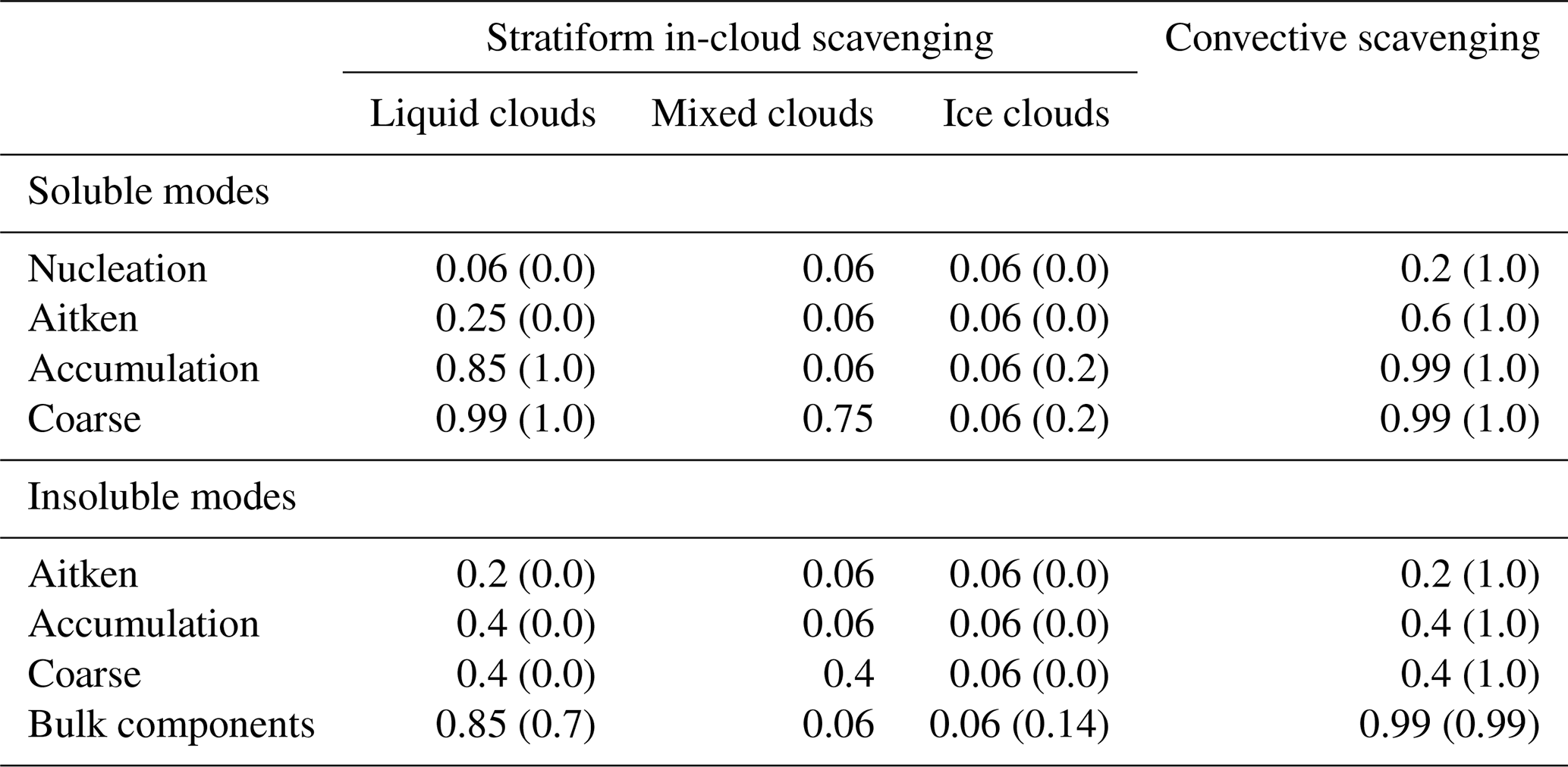
Table 3 Number and mass scavenging coefficients (mm⁻¹) for stratiform below-cloud scavenging. The numbers in parentheses indicate the values used in the TM5 and EC-Earth versions documented in van Noije et al. (2014).

The wet removal of aerosols by clouds and precipitation is described as in the TM5 and EC-Earth versions documented in van Noije et al. (2014) but with updated removal efficiencies, as indicated in Tables 2 and 3. Scavenging of aerosols by precipitation formation in convective and stratiform clouds is described using prescribed mode-dependent scavenging fractions (Croft et al., 2010), which are taken from Stier et al. (2005) for convective clouds and from Bourgeois and Bey (2011) for stratiform clouds (see Table 2). For stratiform clouds, a distinction is made between liquid, mixed, and ice clouds. Here, it is assumed that clouds are liquid at temperatures above 0 ^∘C, ice below −35 ^∘C, and mixed in between. Below-cloud scavenging of aerosols by stratiform precipitation is described using prescribed scavenging coefficients for the particle number and mass in each mode (see Table 3). These coefficients have been estimated from results presented by Croft et al. (2009), obtained for a standard Marshall–Palmer rain droplet size distribution and a precipitation rate of 1 mm h⁻¹. Because different coefficients are applied to particle number and mass, below-cloud scavenging shifts the size distributions of the modes: the nucleation and Aitken modes are shifted to larger sizes, and the accumulation and coarse modes to smaller sizes. All scavenging processes act with the same rate on the bulk aerosol components (ammonium, nitrate, MSA, and lead 210) as on the other components contained in the soluble accumulation mode.

As in earlier versions of the model, the scavenging by precipitation formation in convective and stratiform clouds and the below-cloud scavenging by stratiform precipitation are calculated in TM5 using surface precipitation fields received from IFS. Convective scavenging is included in the convective mass transport operator (see Vignati et al., 2010b). Details on the procedure to calculate the vertical distribution of stratiform precipitation are given in de Bruine et al. (2018). Moreover, in-cloud and below-cloud scavenging by stratiform clouds is reduced by delaying the subgrid-scale mixing between cloudy and cloud-free regions (see Vignati et al., 2010b). The corresponding mixing timescale has been made dependent on the horizontal resolution; at the resolution applied in EC-Earth3-AerChem, it has been increased from 3 to 6 h.

The calculation of the removal of aerosols by sedimentation and surface dry deposition follows the description given by Aan de Brugh et al. (2011). Here, distinct rates are also applied to the particle number and mass in each mode. Compared with the version documented by van Noije et al. (2014), dry deposition and sedimentation of ammonium, nitrate, and MSA have been added. These are now removed at the same rate as the other components contained in the soluble accumulation mode.

The aerosols simulated by TM5 are tropospheric in the sense that they mainly originate from surface emissions and sources in the troposphere. TM5 does not include emissions from explosive volcanoes, which may reach the stratosphere when the eruption is sufficiently strong, or chemical processes that are specifically relevant for particle formation in the stratosphere, such as the production of sulfuric acid by the oxidation of carbonyl sulfide (COS). TM5 does simulate the transport of particles across the tropopause and in the stratosphere, but it cannot be assumed to provide accurate information on stratospheric aerosols. For this reason, IFS does not make use of any aerosol data from TM5 at levels above the model tropopause. Instead, radiative effects of stratospheric aerosols are accounted for in RRTMG_SW and RRTMG_LW using prescribed radiative properties from CMIP6. The treatment of stratospheric aerosols and the calculation of the tropopause level in IFS are identical to the implementation in EC-Earth3 (see Döscher et al., 2021).

The calculation of aerosol optical properties in TM5 is based on Mie theory (van Noije et al., 2014). The extinction, single-scattering albedo, and asymmetry factor are derived for each mode at a number of predefined wavelength values, using a pre-calculated lookup table (Aan de Brugh et al., 2011; Aan de Brugh, 2013). Spectral refractive indices of the various aerosol components are prescribed using input tables from three different sources. For modes consisting of internally mixed particles, effective refractive indices are calculated using volume mixing rules derived from effective-medium theory. Sulfate, organic aerosols, sea salt, ammonium nitrate, MSA, and water are treated as homogeneous mixtures described by the Bruggeman mixing rule. When black carbon, dust, or both are present in the mix, these are treated as inclusions in a homogeneous background medium, using the Maxwell Garnett mixing rule.

The refractive indices of sulfate and sea salt are from the OPAC (Optical Properties of Aerosols and Clouds; Hess et al., 1998) package. The values for sulfate were obtained for a solution consisting of 75 % H₂SO₄ in water. The volume occupied by sulfate is calculated in the optics module of TM5 by assuming that all sulfate is present in the form of sulfuric acid. The refractive indices of MSA and ammonium nitrate are assumed to be the same as for sulfate. For black carbon, the refractive index is prescribed using the corresponding input table from OPAC but with the real and imaginary parts scaled by $\mathrm{1.85}/\mathrm{1.75}$ and $\mathrm{0.71}/\mathrm{0.44}$, respectively. By applying these scale factors, the refractive index at 550 nm is changed from the OPAC value of 1.75 + 0.44i, used in previous versions of the model, to 1.85 + 0.71i, i.e., the mid-range value proposed by Bond and Bergstrom (2006). The refractive indices of organic aerosols and mineral dust are taken from the aerosol–climate model ECHAM-HAM (see Zhang et al., 2012). For OA, the values are based on OPAC; for dust, the imaginary part in the visible part of the spectrum is much lower than in OPAC. The refractive index of water is taken from Segelstein (1981). The corresponding values at 550 nm are given in Table 1.

The resulting aerosol optical properties are input to the photolysis scheme of TM5 (see Sect. 2.3) and the shortwave radiation scheme of IFS (RRTMG_SW). Within each spectral band, the optical properties are calculated at a single wavelength value. For the photolysis scheme, these are the `central' wavelength values defined within the scheme. For RRTMG_SW, they are solar-weighted band averages, with the solar spectral irradiance distribution acting as the weighting function. The corresponding wavelength values are 257, 313, 398, 530, 697, 973, 1269, 1447, 1767, 2040, 2308, 2752, 3407, and 5254 nm. For diagnostic purposes, the optical properties are also determined at a limited number of additional wavelengths (440, 550, and 870 nm). In accordance with the CMIP6 data request, the contributions from the stratosphere are not included in the output optical property fields.

Absorption of longwave radiation by tropospheric aerosols is included in RRTMG_LW using a simplified approach that makes use of precomputed mass attenuation coefficients (MACs) from the prognostic aerosol scheme developed in IFS by Morcrette et al. (2009). The aerosol components represented in this scheme are sulfate, black carbon, organic aerosols, sea salt, and mineral dust. For black carbon and organic aerosols, the hydrophobic and hydrophilic components are treated separately. Sea salt and dust are represented using three size bins. For sea salt, the dry particle diameter ranges are 0.03–0.5, 0.5–5, and 5–20 µm; for dust, the ranges are 0.03–0.55, 0.55–9, and 9–20 µm.

For each of the tracers used in the scheme of Morcrette et al. (2009), wavelength-dependent MACs are specified, which are defined as the extinction cross section per unit dry mass. Thus, the LW absorption in our model is calculated by mapping the modal dry component masses simulated by TM5 onto these tracers. For sea salt and dust, all of the mass contained in the accumulation modes is put into the first bin; of the mass in the coarse modes, 22.2 % is put into the second bin, and the rest is put into the third bin. This percentage is based on the assumption that the third bin contains roughly 3.5 times more mass than the second (Morcrette et al., 2009). The aerosol water simulated by TM5 is not used in this calculation. Instead, water uptake by sulfate, hydrophilic organic aerosols, and sea salt is taken into account via a dependence of their MACs on relative humidity. For BC, the humidity-independent MAC for the hydrophobic component is applied to both the soluble and insoluble modes. The contributions of ammonium nitrate and MSA to the LW absorption are neglected.

Aerosol activation (i.e., the formation of cloud droplets by heterogeneous nucleation on aerosols) is described following the activation scheme from Abdul-Razzak and Ghan (2000), which was specifically developed for modal aerosol schemes like M7. It makes use of Köhler theory to calculate the critical supersaturation and critical particle diameter for each of the relevant water-soluble modes, assuming uniform internal mixing inside the modes. The hygroscopicity parameters adopted in the model for the various aerosol components are given in Table 1. The scheme utilizes an approximate expression to calculate the maximum supersaturation for an air parcel rising adiabatically at a constant vertical velocity. This allows one to estimate the diameter of the smallest activated particle per mode and, consequently, the number of activated particles, as a function of updraft velocity. The cloud droplet number concentration (CDNC) follows as the total in-cloud number concentration of activated aerosols, which is determined by averaging over an appropriate probability distribution of updraft velocities. In EC-Earth3-AerChem and other EC-Earth3 configurations, subgrid-scale vertical velocities are described by a Gaussian distribution with a mean equal to the large-scale vertical velocity (see, e.g., Morales Betancourt and Nenes, 2010). The standard deviation of the distribution is set to 0.8 m s⁻¹. The activation is determined as an average over the range of positive velocities. Currently, this range is sampled using 10 evenly distributed values, varying from 0.2 to 3.8 times the standard deviation. A minimum CDNC value of 30 cm⁻³ is assumed.

For radiation calculations, the effective radius of cloud droplets is determined from the cloud liquid water content provided by the prognostic cloud scheme and the cloud droplet number concentration (CDNC) from the diagnostic activation scheme, following Martin et al. (1994) with the drizzle correction from Wood (2000). The resulting droplet effective radius depends on the simulated aerosol number and mass concentrations, which is an expression of the first aerosol indirect or cloud albedo effect (Twomey, 1977). To prevent unrealistic values, the effective radius is clipped to 4–30 µm.

Autoconversion of cloud droplets into rain is treated using a formulation based on Sundqvist (1978). The rate of precipitation formation by autoconversion in stratiform clouds is calculated as

$$\begin{array}{}\text{(1)}& S=c_{\mathrm{0}}\times q\times \left(\mathrm{1}-\exp \left[-{\left({\displaystyle \frac{q}{q_{\mathrm{c}}}}\right)}^{\mathrm{2}}\right]\right),\end{array}$$

where $c_{\mathrm{0}}^{-\mathrm{1}}$ is a characteristic timescale, q is the cloud liquid water content, and q_c is a critical cloud liquid water content at which the autoconversion starts to be efficient. The calculation of q_c and c₀ in EC-Earth3-AerChem and other EC-Earth3 configurations differs from that in IFS cycle 36r4. Instead of using fixed values of q_c over land and ocean as in the original IFS model, a critical volume-mean cloud droplet radius is specified (see, e.g., Rotstayn and Penner, 2001). As a result, q_c is directly proportional to the CDNC. The value of the critical droplet radius was determined during the tuning of EC-Earth3 and is set to 8.75 µm (see Sect. 3). An additional, weaker dependence on the CDNC is introduced via the rate coefficient c₀ (see Wyser et al., 2020). In accordance with other studies (e.g., Rotstayn and Penner, 2001), c₀ is assumed to vary as $N_d^{-\mathrm{1}/\mathrm{3}}$, where N_d denotes the CDNC. With these modifications, the precipitation formation rate in stratiform clouds is made dependent on the simulated aerosol number and mass concentrations in such a way that the precipitation formation efficiency, $S/q$, is reduced at a larger CDNC. This is an expression of the second aerosol indirect or cloud lifetime effect (Albrecht, 1989).

2.3 Atmospheric chemistry and boundary conditions for chemical tracers

EC-Earth3-AerChem simulates the microphysical and chemical interaction of aerosols and trace gases in the troposphere. The chemistry scheme of TM5 accounts for gas-phase, aqueous-phase, and heterogeneous chemistry (van Noije et al., 2014). The gas-phase reaction scheme is a modified version of the CB05 carbon bond mechanism (Yarwood et al., 2005). A first version of the modified scheme (mCB05) was presented by Williams et al. (2013). The scheme employed in EC-Earth3-AerChem is the extended and updated version described by Williams et al. (2017). Photolysis rates are calculated using the modified band approach from Williams et al. (2006, 2012, 2017).

When calculating photolysis rates, scattering and absorption by aerosols are accounted for based on the online simulated optical properties from within TM5 (see Sect. 2.2), without making use of the stratospheric aerosol forcing data set from CMIP6. As a consequence, the radiative effects of large volcanic eruptions are not explicitly accounted for in the photochemistry of the model. Effects of cloud liquid water and ice particles on photolysis rates are included as described by Williams et al. (2012), but with cloud droplet effective radii calculated following the parameterization of Martin et al. (1994), using fixed values of the CDNC over land and ocean (313.2 and 42.0 cm⁻³, respectively, corresponding to aerosol concentrations of 900 and 40 cm⁻³ for particles with diameters in the range of 0.1–3 µm), with lower and upper limits set to 4 and 16 µm.

Heterogeneous chemistry is limited to the reactive uptake of dinitrogen pentoxide (N₂O₅) at the surface of cloud droplets, ice particles, and aerosols, and the uptake of the hydroperoxyl (HO₂) and nitrate (NO₃) radicals on aerosols. In these reactions one molecule of N₂O₅ produces two molecules of nitric acid (HNO₃), one molecule of NO₃ produces one molecule of HNO₃, and two molecules of HO₂ produce one molecule of H₂O₂. These reactions are described using a first-order rate coefficient, which for a mono-disperse distribution of spherical particles of radius r is given by

$$\begin{array}{}\text{(2)}& \mathrm{d}k\left(r\right)={\left({\displaystyle \frac{r}{D_{\mathrm{g}}}}+{\displaystyle \frac{\mathrm{4}}{v\mathit{\gamma }}}\right)}^{-\mathrm{1}}\mathrm{d}S\left(r\right),\end{array}$$

where D_g is the gas-phase molecular diffusion coefficient of the reacting species in air, v is the mean molecular speed of the species in the gas phase, γ is the probability that a molecule impacting the surface undergoes reaction, and dS(r) is the surface area density of the particles per unit volume of air (see, e.g., Jacob, 2000). The first term in parentheses on the right-hand side of the equation describes the uptake associated with diffusion to the particle surface, and the second term describes the uptake associated with free molecular motion to the particle surface.

Following Huijnen et al. (2014), the uptake of N₂O₅ by heterogeneous reactions in clouds is determined from Eq. (2) by replacing the variable r in the diffusion term with the effective radius r_e of the droplets or ice particles, respectively. Thus, the total rate coefficient is expressed as

$$\begin{array}{}\text{(3)}& k={\left({\displaystyle \frac{r_{\mathrm{e}}}{D_{\mathrm{g}}}}+{\displaystyle \frac{\mathrm{4}}{v\mathit{\gamma }}}\right)}^{-\mathrm{1}}S,\end{array}$$

where S is the total surface area density of the liquid or ice contained in the cloud. The effective radii and surface area densities are calculated as in Williams et al. (2017). In Eq. (3), a temperature-dependent reaction probability γ(T) is used for the uptake of N₂O₅ on liquid water (Ammann et al., 2013), and a fixed γ value of 0.02 is adopted for the uptake on ice particles (Crowley et al., 2010).

For aerosols, the uptake tends to be limited by free molecular motion (Jacob, 2000). Therefore, when performing the integration of Eq. (2) over particle size and composition, we replace $\left(\frac{r}{D_{\mathrm{g}}}+\frac{\mathrm{4}}{v\mathit{\gamma }}\right)$ for all particles in mode i with $\left(\frac{r_{\mathrm{g},i}}{D_{\mathrm{g}}}+\frac{\mathrm{4}}{v{\mathit{\gamma }}_i}\right)$, where r_g,i is the geometric mean (i.e., median) radius of the mode, and γ_i is the reaction probability for that mode. Thus, the total rate coefficient is given by

$$\begin{array}{}\text{(4)}& k={\sum }_i{\left({\displaystyle \frac{r_{\mathrm{g},i}}{D_{\mathrm{g}}}}+{\displaystyle \frac{\mathrm{4}}{v{\mathit{\gamma }}_i}}\right)}^{-\mathrm{1}}{S}_i,\end{array}$$

where S_i is the total surface area density of the particles contained in mode i. For simplicity, the uptake on aerosols is described using constant values of the reaction probability, irrespective of mode or composition. For N₂O₅, a value of 0.02 is assumed, which corresponds to the global mean value from Evans and Jacob (2005); the reaction probabilities for HO₂ and NO₃ are set to 0.06 and 0.001, respectively, based on Abbatt et al. (2012) and Jacob (2000).

The model includes aqueous-phase reactions for the oxidation of total dissolved sulfur dioxide by dissolved hydrogen peroxide (H₂O₂) and ozone, depending on the acidity of the droplets (van Noije et al., 2014). The acidity calculation is done with a spatially homogeneous CO₂ mixing ratio, which is set equal to the annual and global mean surface value provided in the CMIP6 historical or scenario data sets (Meinshausen et al., 2017, 2020).

Other boundary conditions are applied to constrain the mixing ratios of ozone, carbon monoxide, nitric acid, and methane in the stratosphere and that of methane in the lower part of the troposphere (Williams et al., 2017). These boundary conditions are applied through Newtonian relaxation (nudging) towards daily varying zonal mean fields, obtained from monthly input data sets by linear interpolation in time. Compared with the description given by Williams et al. (2017), the boundary conditions applied for ozone and methane have been modified for CMIP6, as described below.

The mixing ratios of ozone in the stratosphere are nudged towards zonal mean fields calculated from the three-dimensional input data sets provided by CMIP6 (Checa-Garcia et al., 2018). For ozone, these consist of a climatology for the preindustrial period and transient data sets for the historical period and the four tier-1 scenarios from the Scenario Model Intercomparison Project (ScenarioMIP; O'Neill et al., 2016). The zonal means from the input files are mapped onto the TM5 grid, using a local mass-conserving regridding scheme in the vertical direction (and linear interpolation in the meridional direction).

The evolution of methane is constrained by the surface mixing ratio data provided by CMIP6 (Meinshausen et al., 2017, 2020). In the lower troposphere, the mixing ratios of methane are nudged towards the zonal means of the CMIP6 fields, using a relaxation time constant of 2.5 ×10⁵ s or 2.9 d (Bândă et al., 2014). The domain where this nudging is applied extends from the surface to the highest model layer with full-level pressure above 550 hPa for a surface pressure of 984 hPa. Area averaging is applied to coarsen the zonal mean input fields from a meridional resolution of 0.5 to 2^∘ in TM5. In the stratosphere, methane is nudged to a climatology derived from measurements made by the HALOE (Halogen Occultation Experiment) satellite instrument (Grooß and Russell, 2005) scaled according to the time series of the annual and global mean surface mixing ratio provided by CMIP6. Following the recommendation of Meinshausen et al. (2017), we assume that there is a delay of 1 year between mixing ratios at the surface and in the stratosphere. Because the HALOE measurements were made from October 1991 to August 2002, we assume that the climatology is representative of the 10-year period from 1992 to 2001, which translates to 1991–2000 at the surface. Thus, the scale factor is defined as the ratio of the global mean mixing ratio in a particular year and the average over the 1991–2000 period.

The ozone and methane mixing ratios from TM5 are input to the SW and LW radiation schemes of IFS. The methane mixing ratios are also used in IFS to determine the production of water vapor by oxidation of methane in the stratosphere. This calculation makes use of the same parameterization as in EC-Earth3 (see Döscher et al., 2021).

2.4 Anthropogenic and natural emissions

This section gives an overview of the emissions of reactive gases and aerosols applied in TM5. The amounts of emissions from anthropogenic activities and open biomass burning are specified using data sets provided by CMIP6 (Feng et al., 2020): historical anthropogenic emissions are taken from the Community Emissions Data System (CEDS; Hoesly et al., 2018), historical fire emissions are taken from the BB4CMIP6 data set (van Marle et al., 2017), and future emissions are taken from the respective scenario data sets (Gidden et al., 2019). Anthropogenic and biomass burning emissions for the historical period are provided as monthly and annually varying fields. An exception is the anthropogenic emissions of methane prior to 1970, for which monthly emissions are only provided at 10-year intervals. Scenario emissions are provided for 2015 and from 2020 onwards, also at 10-year intervals. For these cases, the emissions in intermediate years are calculated by linear interpolation.

Biogenic emissions of non-methane volatile organic compounds (NMVOCs) and carbon monoxide (CO) are prescribed using monthly estimates from the MEGAN-MACC data set (Sindelarova et al., 2014) for the year 2000, which was produced by the Model of Emissions of Gases and Aerosols from Nature (MEGAN) version 2.1 under the Monitoring Atmospheric Composition and Climate (MACC) project. Distinct diurnal cycles are applied to the biogenic emissions of isoprene and monoterpenes (Bergman et al., 2021). Speciated anthropogenic NMVOC emissions are provided for all sources, except for the aircraft sector. Following the recommendations from the CEDS team, the NMVOC emissions from the aircraft sector are split using distinct NMVOC profiles for the contributions from in-flight exhaust and takeoff and landing. Natural methane emissions and the rate coefficients describing the uptake of methane by soils are prescribed using estimates from Spahni et al. (2011) for the year 2000. The sources of mineral dust and sea salt, the oceanic source of DMS, and the production of nitrogen oxides (NO_x) by lightning are calculated online, as described below. All other natural emissions are prescribed as documented in van Noije et al. (2014). These include terrestrial DMS emissions from soils and vegetation, biogenic emissions of NO_x and ammonia (NH₃) from soils, oceanic emissions of CO, NMVOCs and NH₃, and SO₂ fluxes from continuously emitting volcanoes.

The dust source is calculated using the scheme developed by Tegen et al. (2002). It is based on the assumption that a particle can be released from the soil when the surface friction velocity exceeds a certain threshold value, which depends on the size of the particle and the roughness of the surface (Marticorena and Bergametti, 1995). The threshold friction velocity is determined using a monthly climatology of roughness lengths derived from scatterometer observations from the European Remote Sensing (ERS) satellite (Prigent et al., 2005; see also Cheng et al., 2008). In grid cells with a substantial fraction of cultivated land, the dust source is enhanced by reducing the threshold friction velocity by up to 27 %, following a similar approach as in Tegen et al. (2004). Currently, the fractional cropland areas assumed in this calculation are based on a data set for 1992 (Ramankutty and Foley, 1999). The vertical flux of dust particles is subsequently calculated as a function of particle size and the 10 m horizontal wind speed following Tegen et al. (2002). The grassland and shrubland area fractions that enter this calculation are determined from the vegetation fields received from IFS. Snow-covered areas are excluded as dust sources; the snow cover is estimated from the snow depth as in Tegen et al. (2002). Soil moisture effects are presently not accounted for.

The vertical flux is calculated for four size bins with radius boundaries at 0.1, 0.3, 0.9, 2.7, and 8.0 µm (actually 8.0 divided by 3ⁿ with the integer number n running from 4 to 0). The resulting size-resolved flux is subsequently mapped to the accumulation and coarse modes of M7 with the respective mass median radius values set to 0.37 and 1.75 µm and respective geometric standard deviation values of 1.59 and 2.0 (Stier et al., 2005). The weights of the distributions are determined such that the respective mass fluxes in the intervals covered by the first bin and by the second to fourth bins are exactly conserved. The mass and number fluxes associated with these two lognormal distributions are put into the insoluble accumulation and coarse modes, respectively. The global dust emission is tuned by applying a constant correction factor to the threshold friction velocity (Tegen et al., 2004; Cheng et al., 2008). This factor has been set to 0.6 (see Sect. 3).

The source of sea salt is calculated following Gong (2003) with a temperature dependence based on Salter et al. (2015). The flux of the number of sea-spray particles formed over ice-free ocean areas is expressed as a function of the particle radius at 80 % humidity and the 10 m horizontal wind speed, U₁₀, using the parameterization from Gong (2003). In this formulation, the ocean whitecap coverage fraction, W, is related to U₁₀ as $W=\mathrm{3.84}\times {\mathrm{10}}^{-\mathrm{6}}\times U_{\mathrm{10}}^{\mathrm{3.41}}$ (Monahan and Muircheartaigh, 1980). This size-resolved flux is approximated by two lognormal distributions with number median dry radius values of 0.09 and 0.794 µm and geometric standard deviation of the accumulation and coarse modes of M7, respectively (Vignati et al., 2010a). The weights of the distributions are determined by requiring that the mapping conserves the integrated number fluxes of particles with dry radius values in the ranges of 0.05–0.5 and 0.5–5 µm. It is assumed that the emitted sea-spray particles consist of sea salt only. The particle number and sea-salt mass fluxes associated with these two lognormal distributions are put into the soluble accumulation and coarse modes, respectively.

Several studies have indicated that the formation of sea spray depends on the sea water temperature and that this temperature dependence changes the size distribution of the formed particles (e.g., Mårtensson et al., 2003; Jaeglé et al., 2011; Ovadnevaite et al., 2014; Salter et al., 2014). Following the approach of Salter et al. (2015), we describe the temperature effect using distinct multiplication factors for the particle fluxes in the accumulation mode, f_a, and coarse mode, f_c. These factors are given by

$$\begin{array}{ll}{\displaystyle }& {\displaystyle }{f}_{\mathrm{a}}\left(T\right)=-\mathrm{8.75593}\times {\mathrm{10}}^{-\mathrm{5}}\times T^{\mathrm{3}}+\mathrm{5.56771}\times {\mathrm{10}}^{-\mathrm{3}}\\ {\displaystyle }& {\displaystyle }\times T^{\mathrm{2}}-\mathrm{0.11670}\times T+\mathrm{1.79321}\\ \text{(5)}& {\displaystyle }& {\displaystyle }\text{ for }-\mathrm{1}\le T\le \mathrm{15}{}^{\circ }\mathrm{C},\end{array}$$

and

$$\begin{array}{ll}{\displaystyle }& {\displaystyle }{f}_{\mathrm{c}}\left(T\right)=\mathrm{3.75294}\times {\mathrm{10}}^{-\mathrm{2}}\times T+\mathrm{0.43706}\\ \text{(6)}& {\displaystyle }& {\displaystyle }\text{ for }-\mathrm{1}\le T\le \mathrm{30}{}^{\circ }\mathrm{C},\end{array}$$

where T is the sea-surface temperature (SST) in degrees Celsius, and coefficients have been rounded to five decimals. No temperature dependence is assumed outside of the indicated ranges. Equations (5) and (6) are simplified forms of the empirically derived polynomial expressions from Salter et al. (2015) for their modes with number median radii of 0.0475 and 0.75 µm, respectively, which have been scaled to 1.0 at a reference SST value of 15 ^∘C. Figure 1 shows the temperature factors f_a and f_c as functions of the SST.

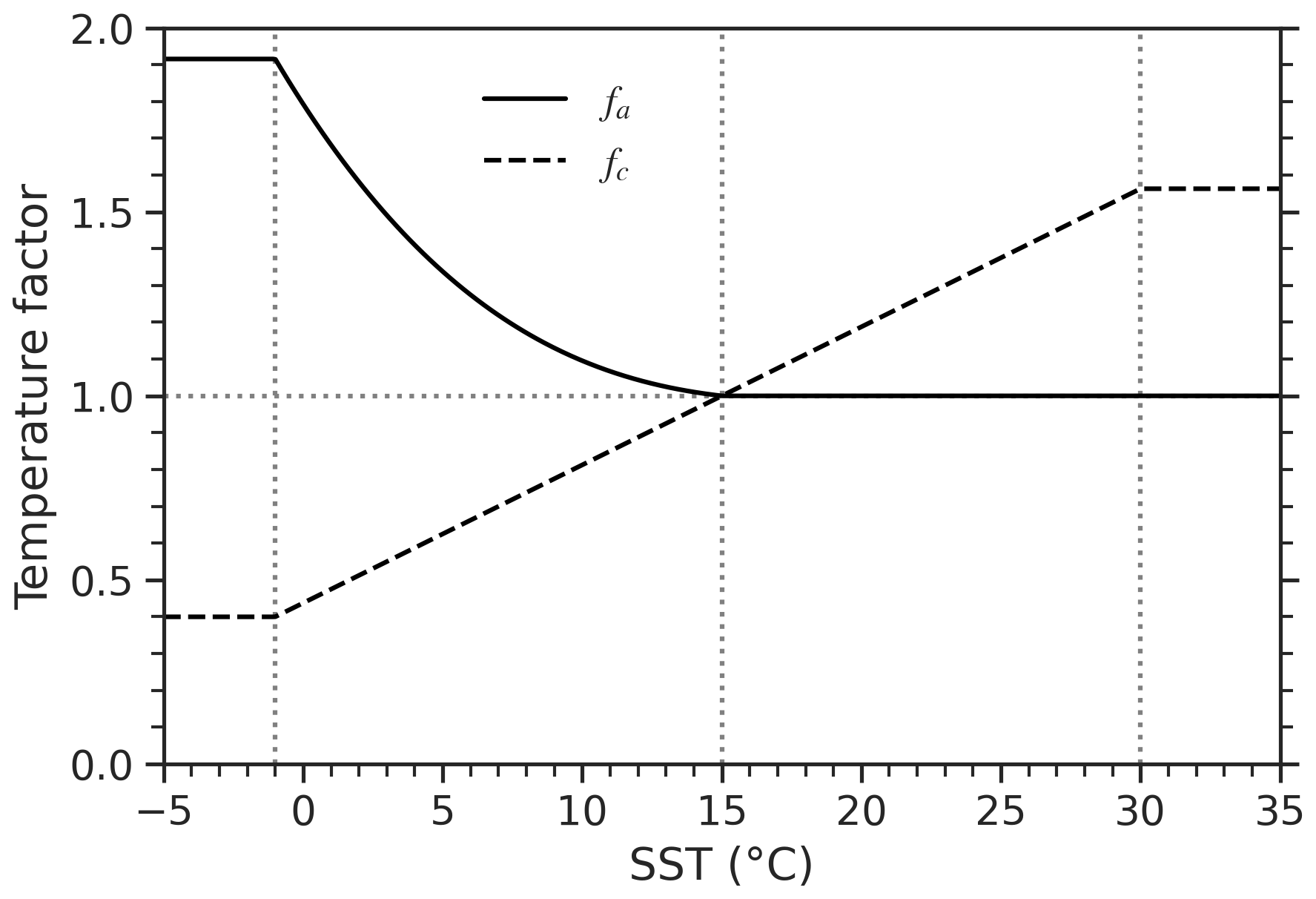
Figure 1 Temperature factors f_a and f_c for the formation of sea-spray particles in the accumulation and coarse modes, respectively.

The DMS flux in ice-free ocean areas can be calculated as the product of the local surface ocean DMS concentration and the gas transfer velocity (e.g., Lana et al., 2011). The ocean concentrations are prescribed according to the monthly climatology from Lana et al. (2011). The gas transfer velocity is parameterized following Wanninkhof (2014). It is proportional to $U_{\mathrm{10}}^{\mathrm{2}}$ and depends on the SST through the Schmidt number. The Schmidt number is expressed as a fourth-order polynomial of the SST.

The amount of NO_x produced in lightning discharges is calculated using an improved version of the parameterization described by Huijnen et al. (2010). Compared with earlier model versions (e.g., Huijnen et al., 2010; van Noije et al., 2014), the distribution between cloud-to-ground (CG) and intra-cloud (IC) discharges has been corrected for clouds for which the thickness of the cold sector is less than 5.5 km. Previously, the percentage of CG discharges was set to 0 % for these clouds; this has now been changed to 100 % (Price and Rind, 1994). As a second revision, it is now assumed that IC flashes are as efficient at producing NO_x as CG flashes (Ridley et al., 2005; Ott et al., 2010). The amount of NO_x produced by each flash is still scaled by a constant factor to ensure that the global total production is around 6 Tg N yr⁻¹ (see Sect. 3).

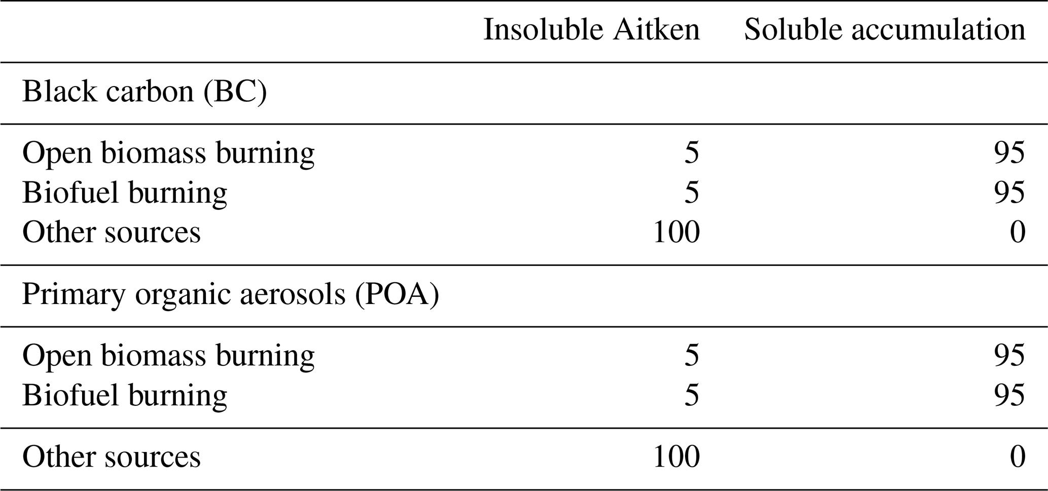
As in earlier versions of the model, the emissions of black carbon, primary organic aerosols, and sulfate are characterized using lognormal size distributions with the same geometric standard deviation as the corresponding modes in M7. Previously, carbonaceous aerosols were emitted in the Aitken modes of M7 using size distributions with a number median radius of 0.040 µm for open biomass burning and 0.015 µm for all other sources (Aan de Brugh et al., 2011). These values were taken from Dentener et al. (2006), without correcting for the fact that the Aitken modes in M7 have a different geometric standard deviation than the distributions recommended in that study. All of the BC emissions were put into the insoluble mode, whereas 65 % of the emitted POA mass was assumed to be water soluble irrespective of the source of the emissions (Stier et al., 2005). In the current model version, the carbonaceous emissions are described using an Aitken-mode distribution for the insoluble particles and an accumulation-mode distribution for the soluble particles (see Table 4). Following Stier et al. (2005), the number median radii of these distributions are set to 0.030 and 0.075 µm, respectively. Carbonaceous emissions from solid biofuel burning and open biomass burning are now assumed to have similar characteristics: for both POA and BC, it is assumed that 95 % of the mass from these sources is emitted in the (soluble) accumulation mode (see Sect. 3). BC and POA emissions from other sources are assumed to be insoluble.

Table 4 Distribution of the carbonaceous aerosol emissions from open biomass burning, biofuel burning, and other sources over the insoluble Aitken and soluble accumulation modes, as mass percentages.

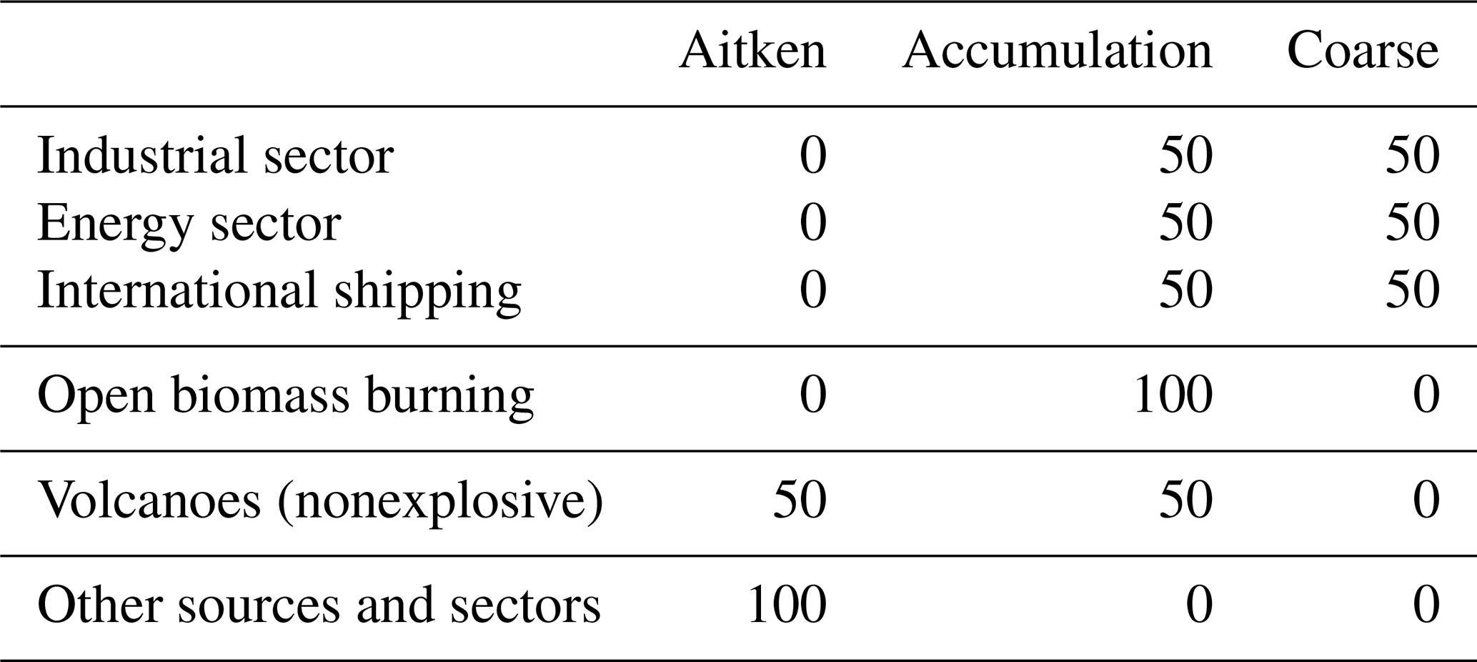
Following the recommendation by Dentener et al. (2006), 2.5 % of the emitted SO_x mass is assumed to be emitted in the form of SO₄ particles. These particulate emissions are distributed over the soluble Aitken, accumulation, and coarse modes, using three lognormal size distributions with number median radii set to 0.030, 0.075, and 0.75 µm, respectively (Stier et al., 2005). The distribution of the emitted SO₄ mass from the various sources and sectors over the three modes has been revised as indicated in Table 5. Previously, all of the emissions from the industrial sector were put into the accumulation mode, while half of the emissions from all other sources and sectors were put into the Aitken mode and the other half were put in the accumulation mode (Aan de Brugh et al., 2011). The new distribution more closely follows the recommendations from Dentener et al. (2006).

Table 5 Distribution of the sulfate emissions from the various sources and sectors over the soluble Aitken, accumulation, and coarse modes, as mass percentages.

All emissions except those from the aircraft sector are provided as two-dimensional fields and are distributed over model layers using the vertical profiles given in Table A1 of van Noije et al. (2014). Here, the emissions from open biomass burning, including those from grassland fires and agricultural waste burning, are distributed according to the profiles defined for forest fires.

2.5 Technical and numerical aspects

The atmospheric grid of TM5 is a regular latitude–longitude grid with a resolution of 3^∘ × 2^∘ (longitude × latitude). The base time step of the model is 1 h, but the time step is dynamically reduced where needed to fulfill the Courant–Friedrichs–Lewy (CFL) stability criterion (Krol et al., 2005; Huijnen et al., 2010). To avoid the need for very short time steps, a reduced grid is applied in the zonal advection routine. In the reduced grid, the number of grid points in the zonal direction gradually decreases when approaching the poles. By merging cells, the number per latitude band is reduced from 120 equatorward of 76^∘ to 40 between 76 and 78^∘, 8 between 78 and 82^∘, 4 between 82 and 88^∘, and 2 between 88 and 90^∘. The TM5 grid consists of 34 hybrid sigma-pressure layers in the vertical direction, which have been constructed by merging layers defined on the IFS grid. Except for the top layer, all layers in TM5 are combinations of two or three adjacent layers in IFS. The top layer corresponds to five layers in IFS and has a full-level pressure of ∼ 0.1 hPa.

Details about the OASIS data exchange between IFS and TM5 are given in van Noije et al. (2014). Their Table 1 gives a list of the atmospheric and surface fields transferred from IFS to TM5. Grid-point atmospheric fields are interpolated from the N128 reduced Gaussian grid to the TM5 3^∘ × 2^∘ grid. To make use of the higher resolution in IFS, surface fields are interpolated to 1^∘ × 1^∘ and applied at this resolution in TM5 to calculate dry deposition velocities and the sources of mineral dust, sea salt, and oceanic DMS. The west–east and south–north components of the 10 m wind are not used by TM5 anymore and have been replaced by the 10 m wind speed; furthermore, the sea-surface temperature, needed in the calculation of the production of sea spray and the oceanic DMS flux, has been added as an instantaneous field.

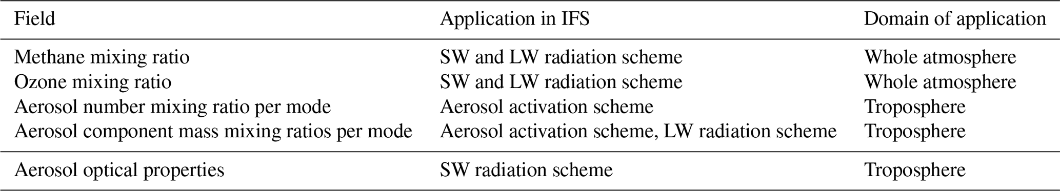
Table 6 lists the fields the IFS receives from TM5 as well as where they are applied. These fields are all three-dimensional and instantaneous. Mass mixing ratios are passed for all M7 components (including OA, but not POA and SOA separately) as well as nitrate and MSA. As nucleation-mode particles play no role in cloud droplet formation and have negligible LW radiative effects, the associated number and mass mixing ratios are not included in the data transfer. The aerosol optical property fields are the extinction, single-scattering albedo, and asymmetry factor at the 14 wavelength bands of the RRTMG SW radiation scheme (see Sect. 2.2). We recall that the model distinguishes between stratospheric and tropospheric aerosols, and that the TM5 aerosol fields are only used by IFS in the troposphere. Therefore, the transfer of aerosol fields and the calculation of the optical fields for RRTMG_SW are limited to the lowest 23 layers (i.e., the domain extending from the surface to 73.4 hPa). The convection calculations in TM5 are limited to the same domain.

Table 6 Fields transferred from TM5 to IFS.

The time interval of the data exchange between IFS and TM5 is 6 h. This is 8 times the time step in IFS and 6 times the base time step in TM5. To put this into perspective, the stand-alone configuration of TM5 has been driven by 6-hourly meteorological fields during many years, and the full radiation computations in IFS (cycle 36r4) are only done every 3 h (Morcrette, 2000). It would be possible to increase the exchange frequency to 3 h, but this would lead to a substantial decline in the computational performance.

Built around the OASIS3-MCT coupler, the synchronization of IFS and TM5 has been overhauled. On the IFS side, it uses the new coupling interface introduced in EC-Earth3 (Döscher et al., 2021). The two models still run concurrently, but TM5 execution is not delayed by a full coupling interval anymore. Indeed, in the previous implementation, TM5 could start simulating the next 6-hourly interval only once IFS had reached the end of it (van Noije et al., 2014). The advantage was that TM5 knew the pressure at the beginning and end of the coupling interval without any lag, and could adjust the horizontal air mass fluxes to close the air mass balance and ensure mass-conserving transport of tracers during that interval (Segers et al., 2002). The new approach removes the 6 h delay, making the execution of TM5 and IFS more synchronous, but it introduces a lag (as defined by OASIS3-MCT) of 45 min for the fields received by TM5 (i.e., one IFS time step). Although only the fields at the beginning of the interval are known now, TM5 still applies a mass-conserving transport operator. This leads to a surface pressure that slightly diverges from its IFS counterpart but is correctly reset at the start of the next coupling interval. The new design has some important advantages. It removes the need to run the models sequentially when the feedback from TM5 to IFS is switched on. Moreover, that feedback occurs with a lag of 1 h (one TM5 time step) instead of 3 h (half a coupling interval) as was previously the case. Equally as important, it greatly facilitates coupling additional components to TM5, like a dynamic global vegetation model and/or an ocean biogeochemistry component. This capability was exploited to develop a carbon-cycle configuration of EC-Earth3 (Döscher et al., 2021).

The large amount of data exchanged with TM5 has always hindered the model performance. Several steps have been taken to alleviate this issue (see Table 7). First, as TM5 runs on a subset of IFS levels, the reduction operation was moved from TM5 to IFS to decrease the amount of multilevel data transferred to TM5, which halved the execution time. An additional 40 % performance increase was obtained by packing several levels together into one OASIS3-MCT entry, taking advantage of the new bundle feature of the coupler (Craig et al., 2017). Finally, the parallelization of TM5 with the Message Passing Interface (MPI) library has been revised. The domain decomposition now consists of a geographical partitioning (Williams et al., 2017). This has strongly improved the scalability of the TM5 model and has also enabled all MPI tasks to communicate with OASIS3-MCT, essentially parallelizing the exchange of grid-point fields. In the model version described by van Noije et al. (2014), only one TM5 core was communicating with OASIS3. Although the transfer of spectral fields cannot be distributed in the same fashion, the multicore coupling of grid-point fields has improved the performance by 35 %. The last improvement stems from limiting the transfer of aerosol fields to 23 out of 34 levels, which corresponds to the domain where convection is applied in TM5 with a top at about 70 hPa.

Table 7 Computational speed in simulated years per day (SYPD) for different implementations of the data exchange between TM5 and IFS. The benchmark tests were primarily conducted on the high-performance computer of the ECMWF. The performance with the final CMIP6 configuration is also reported for additional platforms of the Swedish Meteorological and Hydrological Institute (SMHI); the IT Center for Science, Finland (CSC); the Royal Netherlands Meteorological Institute (KNMI); and the Swedish National Supercomputer Centre (NSC).

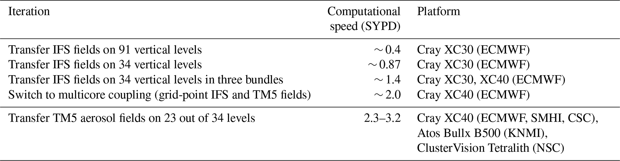
In its latest iteration with load balancing and optimization of bundle sizes, EC-Earth3-AerChem runs at about 3 simulated years per day (SYPD; Balaji et al., 2017) on the most recent platforms. This can be compared to the standard EC-Earth3 model and its high-resolution configuration, which typically reach 15–20 and 2–4 SYPD (Haarsma et al., 2020), respectively. Clearly, performance-wise, the increased complexity from interactive aerosols and atmospheric chemistry costs about as much as increasing the horizontal resolution of the model (by a factor of 2 and 4 for the atmosphere and ocean components, respectively).

3 Tuning and spin-up

As a first step in the tuning process, a small number of parameters in TM5 were optimized in a stand-alone configuration driven by meteorological and surface fields from the ERA-Interim reanalysis (Dee et al., 2011) using the same horizontal resolution and number of vertical levels as in EC-Earth3-AerChem (see van Noije et al., 2014). Specifically, the correction factor for the threshold friction velocity applied in the calculation of the mineral dust source was set to 0.6, resulting in a global emission of 1.12 × 10³ Tg for the year 2010. This is well within the range obtained in other global models (e.g., Huneeus et al., 2011; Gliß et al., 2021) and yields reasonable values of aerosol optical depth in regions affected by dust. Note that for a proper comparison of emitted mass amounts from different models one should account for differences in the representation of the upper end of the size distribution. Moreover, the scale factor applied to the NO_x produced in lightning flashes was determined from the requirement that the total production in 2006 is 6.0 Tg N. The assumptions about the size distribution and solubility of carbonaceous aerosols emitted from biofuel and open biomass burning have also been revised as part of the tuning. Initially, 65 % of the organic matter from open biomass burning was assumed to be water soluble, consistent with observations (Mayol-Bracero et al., 2002; Reid et al., 2005). POA emissions from other sources, including solid biofuel burning, as well as freshly emitted BC were assumed to be 100 % insoluble and, thus, emitted in the Aitken mode. This resulted in overly high particle number concentrations in residential regions with substantial biofuel burning, in particular in Asia but also in Europe during winter. The carbonaceous emissions from solid biofuel burning have, therefore, been separated from the other emissions in the residential sector and are treated as emissions from open biomass burning. In an intermediate version of the model, 50 % of the BC mass emitted by biofuel and biomass burning was assumed to be emitted into the (soluble) accumulation mode (see, e.g., Kodros et al., 2015). In line with measurements of the size distributions of emissions from open biomass burning (Janhäll et al., 2010) and biofuel burning (Li et al., 2009; Winijkul et al., 2015), this percentage was later been increased to 95 % for both POA and BC. This revision has led to modest reductions in the aerosol optical depth in parts of East Asia and, during boreal winter and spring, in western Africa and the tropical Atlantic, improving the comparison with observations in these regions (not shown). An evaluation of aerosol optical properties for the year 2010 simulated with the final parameter settings in TM5 is presented by Gliß et al. (2021). This evaluation includes both the TM5 stand-alone configuration driven by meteorological and surface fields from the ERA-Interim reanalysis (Dee et al., 2011) and the EC-Earth3-AerChem model in atmosphere-only configuration with sea-surface temperatures (SSTs) and sea-ice concentrations prescribed as in the Atmospheric Model Intercomparison Project (AMIP) experiment (Döscher et al., 2021) and atmospheric winds and surface pressures nudged to ERA-Interim fields.

The tuning of the model's climate started from the tuned configuration of EC-Earth3 (Döscher et al., 2021). As explained in Sect. 1, the main differences between the two configurations are due to tropospheric aerosols and tropospheric and lower-stratospheric ozone. In EC-Earth3, tropospheric aerosols are described by the MACv2-SP simple plume representation of anthropogenic aerosol optical properties and cloud effects (Stevens et al., 2017) in combination with a preindustrial climatology produced by TM5.

EC-Earth3 produces an aerosol effective radiative forcing (ERF) of about −0.8 W m⁻² over the CMIP6 historical period (1850–2014), as estimated from a set of 30-year atmosphere-only simulations performed as part of the Radiative Forcing Model Intercomparison Project (RFMIP; Pincus et al., 2016). For comparison, using the same IFS parameter settings as in EC-Earth3, the aerosol ERF in EC-Earth3-AerChem was estimated at −1.1 W m⁻². The final revision of the treatment of carbonaceous emissions from biofuel and biomass burning emissions resulted in a ∼ 0.4 W m⁻² weaker aerosol forcing, bringing the forcing in EC-Earth3-AerChem closer to that in EC-Earth3. This is mainly due to a reduction in the SW cloud radiative forcing, as we have verified using the method proposed by Ghan (2013). (The aerosol ERF estimates for both configurations were obtained from 15-year simulations with AMIP SSTs and sea-ice concentrations for the years 2000–2014, as the difference in the net energy imbalance at the top of the atmosphere between simulations with emissions for 2000–2014 and 1850, respectively. To isolate the effects of tropospheric aerosols, the mixing ratios of methane and ozone in these simulations were prescribed in IFS as in EC-Earth3.)

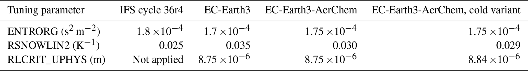
In view of these results, our tuning efforts focused on the preindustrial climate of EC-Earth3-AerChem; no attempt was made to make specific adjustments to improve the model's climate for the present day or the simulated warming over the historical period. When tuning the preindustrial climate of EC-Earth3-AerChem, a small number of atmospheric tuning parameters in IFS were readjusted, leaving ocean and sea-ice parameters in NEMO untouched. The model was initialized from the IFS and NEMO states taken from the EC-Earth3 preindustrial control simulation (member r1i1p1f1, after 500 years), and a TM5 state representative of preindustrial conditions. (After 10 years, a small update of the preindustrial vegetation climatology was introduced. This had only a minor impact on the simulated preindustrial climate.) Without readjusting any tuning parameters in IFS, the model started to drift to a new climate state, characterized by higher temperatures especially in the Northern Hemisphere. The increase in zonal mean surface air temperatures varied from less than a few tenths of a degree in the midlatitudes of the Southern Hemisphere to a few degrees at high latitudes in the Northern Hemisphere. A comparison with the ERA5 reanalysis for the 1980s (Herschbach et al., 2020), corrected for the observed warming since preindustrial times, indicated that the cold biases of EC-Earth3 turned into warm biases over large areas of the Northern Hemisphere. We tried to reduce these warm biases by readjusting a small set of tuning parameters in IFS. Based on experience gained during the tuning of EC-Earth3 (Döscher et al., 2021), three parameters were selected that affect both warm and cold regions: ENTRORG, the fractional entrainment (m⁻¹) for positively buoyant deep convection divided by the gravitational constant; RSNOWLIN2, which governs the temperature dependence of the autoconversion of ice crystals to snow in large-scale precipitation (Lin et al., 1983); and RLCRIT_UPHYS, the critical cloud droplet radius for the autoconversion of droplets into rain in large-scale precipitation (see Sect. 2.2). Using parameter sensitivities derived from EC-Earth3 atmosphere-only simulations, two combinations of settings were defined corresponding to a target global mean surface cooling of 0.5 and 0.75 ^∘C (see Table 8).

Table 8 Parameter settings for the three IFS parameters that have been readjusted for tuning the model's preindustrial climate. The column labeled “EC-Earth3-AerChem” contains the values adopted in the CMIP6 configuration of the model, which correspond to a target reduction in the global mean surface temperature of 0.5 ^∘C compared with the configuration with the standard EC-Earth3 settings. The settings indicated in the column labeled “EC-Earth3-AerChem, cold variant” correspond to a target surface cooling of 0.75 ^∘C.

Initially, the focus was on the cold variant of the model. A sensitivity simulation for this configuration was started by branching off from the reference simulation with standard EC-Earth3 settings (after about 20 years from the start). As expected, the configuration with adjusted settings produced a colder climate. The Northern Hemisphere was more strongly affected than the Southern Hemisphere: at northern high latitudes, the zonal mean surface air temperature was reduced by more than 2 ^∘C. After another ∼ 100 years, a third simulation was started with parameter settings as in the final EC-Earth3-AerChem configuration (see Table 8). This simulation branched off from the reference simulation. After having completed a few decades, the reference simulation was stopped, and the two sensitivity simulations were continued for another ∼ 90 years. At that point, it was discovered that the correction factor for the dust source was set to 0.7, a value obtained for an intermediate version of EC-Earth3-AerChem, resulting in a reduction of the global source to about 550 Tg yr⁻¹ in these simulations. After resetting the factor to the intended value of 0.6, a new set of simulations was launched for the three configurations indicated in Table 8. This increased the dust source to about 1.1 ×10³ Tg yr⁻¹, as verified from the first few years of the simulations. The configuration with a cooling target of 0.5 ^∘C produced satisfactory behavior for the same set of atmosphere and ocean variables considered in the tuning of EC-Earth3 (Döscher et al., 2021) and was spun up for 300 years. Compared with EC-Earth3, this configuration produced higher, more realistic preindustrial temperature levels in the Northern Hemisphere, resulting in reduced long-term variability in the global mean surface temperature. While running the CMIP6 historical simulation with the selected parameter settings, another bug was discovered in the code dealing with the stratospheric aerosols. This bug affected only EC-Earth3-AerChem and led to spurious warming by absorption of SW radiation in the stratosphere. This resulted in a completely incorrect response to large volcanic eruptions. After fixing this bug, the preindustrial spin-up simulation was continued for another 150 years. The impact of the bug fix on preindustrial surface climate turned out to be small. This completed the tuning and spin-up of the model, totaling 770 continuous years for the final configuration (on top of the EC-Earth3 preindustrial control simulation).

4 Results

In this section, we present results from some of the core CMIP6 simulations conducted with EC-Earth3-AerChem. Here, we only include results from simulations with active ocean and sea-ice components. An analysis of the AMIP simulation and AerChemMIP atmosphere-only simulations will be presented elsewhere. The CMIP6 historical simulation is compared against observational data sets, using all four available realizations (see Sect. 4.3). For other experiments, the EC-Earth3-AerChem results presented in this paper are based on a single realization (r1i1p1f1). When reporting statistics, the mean and standard deviation (SD) of a variable will be given as “mean (SD)”, whereas the mean and standard error of the mean (SEM) will be denoted by “mean ± SEM”.

4.1 Preindustrial control simulation

Figure 2 shows time series of annual means from the model's 500-year-long preindustrial control simulation (piControl) for the global surface air temperature, the global net radiative flux at the top of the atmosphere, and the strength of the Atlantic meridional overturning circulation at 26^∘ N. The corresponding time series from an equally long control simulation performed with the standard EC-Earth3 configuration (realization r1i1p1f1) have been included for comparison.

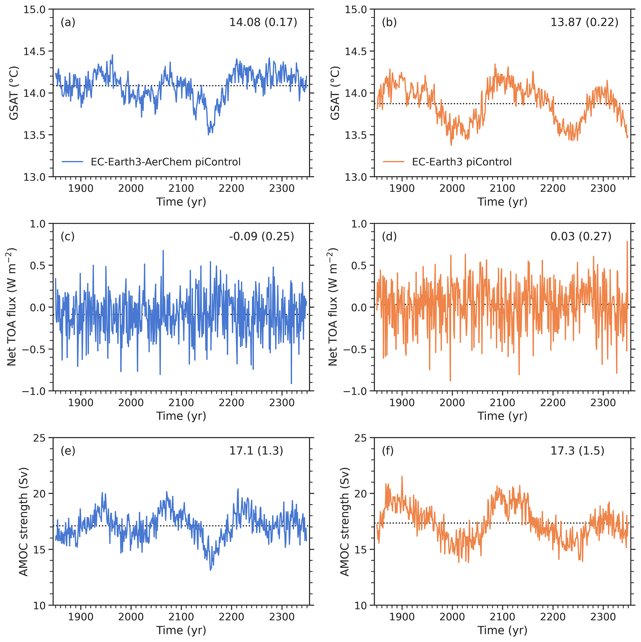
Figure 2 Time series of the global surface air temperature (GSAT), the global net radiative flux at the top of the atmosphere (TOA), and the strength of the Atlantic meridional overturning circulation (AMOC) at 26^∘ N in the preindustrial control simulation (piControl) of EC-Earth3-AerChem and EC-Earth3. All data points are annual means; the numbers given in the top right of each panel are the mean and interannual standard deviation.

The global surface air temperature (GSAT) in the EC-Earth3-AerChem simulation is on average 14.08 ^∘C. The spread in annual values has a standard deviation of 0.17 ^∘C. The linear trend in GSAT is 0.015 ± 0.005 ^∘C per century, which is small but statistically significant. The mean net energy imbalance at the top of the atmosphere (TOA) is −0.09 W m⁻² with an interannual standard deviation of 0.25 W m⁻². The drift in the TOA flux is statistically insignificant at the p=0.05 level (3.5 ± 7.8 mW m⁻² per century).

The mean GSAT in the EC-Earth3 simulation is 13.87 ^∘C with an interannual standard deviation of 0.22 ^∘C. Hence, in agreement with the goals set during the tuning phase, EC-Earth3-AerChem is on average slightly warmer (0.21 ± 0.01 ^∘C) and exhibits lower internal variability than EC-Earth3.

Both configurations display substantial low-frequency variability on centennial timescales. The dominant period in GSAT is ∼ 220 years in EC-Earth3 and ∼ 130 years in EC-Earth3-AerChem. In both configurations, there is a clear correlation between the long-term evolution of GSAT and the strength of the Atlantic meridional overturning circulation (AMOC), with a lag or lead time of at most a few years. The Pearson correlation coefficient between the annual mean GSAT and the concurrent AMOC strength at 26^∘ N is 0.49 for EC-Earth3-AerChem and 0.74 for EC-Earth3. After removing the higher frequencies by applying a 10-year moving average to the time series, the correlation coefficients increase to 0.731 and 0.919, respectively. The cross-correlation function between the smoothed GSAT and AMOC time series peaks at 0.734 for a lag time of 2 years for EC-Earth3-AerChem and at 0.926 for a lag time of −3 years for EC-Earth3, where a positive lag indicates that the AMOC is leading. Thus, in both configurations most of the interdecadal variance in GSAT can be explained by variations in the AMOC strength: ∼ 54 % in EC-Earth3-AerChem versus ∼ 86 % in EC-Earth3.

In both configurations, a weakening of the AMOC is associated with reduced deep-water formation by convective mixing in the Labrador Sea, as diagnosed from the local mixed-layer depth (Griffies et al., 2016; not shown). This supports the idea that the mechanism underlying the long-term variability in EC-Earth3-AerChem is similar to that in other EC-Earth3 configurations displaying spurious interdecadal variability in preindustrial and historical simulations (Döscher et al., 2021; Parsons et al., 2020). As discussed in Sect. 5, we believe this instability is related to the use of the NEMO3.6 ocean model and the relatively coarse ORCA1 grid (Koenigk et al., 2020).

In Fig. 3, we compare the spatial distribution of the mean and interannual variability in surface air temperatures from the two control simulations. EC-Earth3-AerChem is significantly warmer over most of the Northern Hemisphere (NH) and is slightly colder over most of the Southern Hemisphere (SH); over the Southern Ocean, both warmer and colder regions can be observed. The mean surface air temperature (SAT) difference is 0.61 ± 0.02 ^∘C in the NH and −0.18 ± 0.01 ^∘C in the SH. The largest differences in mean temperatures are found over the Barents Sea, the Nordic Seas, and the Labrador Sea. In these regions, the preindustrial mean SAT is several degrees higher in EC-Earth3-AerChem (up to 4.6 ^∘C). The higher temperatures simulated by EC-Earth3-AerChem in the Arctic Ocean and North Atlantic are in better agreement with observational estimates for the late 19th century (not shown). The same is true for the zonal mean temperatures at all latitudes north of ∼ 10^∘ N, except for the band between ∼ 40 and 50^∘ N (see Sect. 4.3 and Fig. 8b).

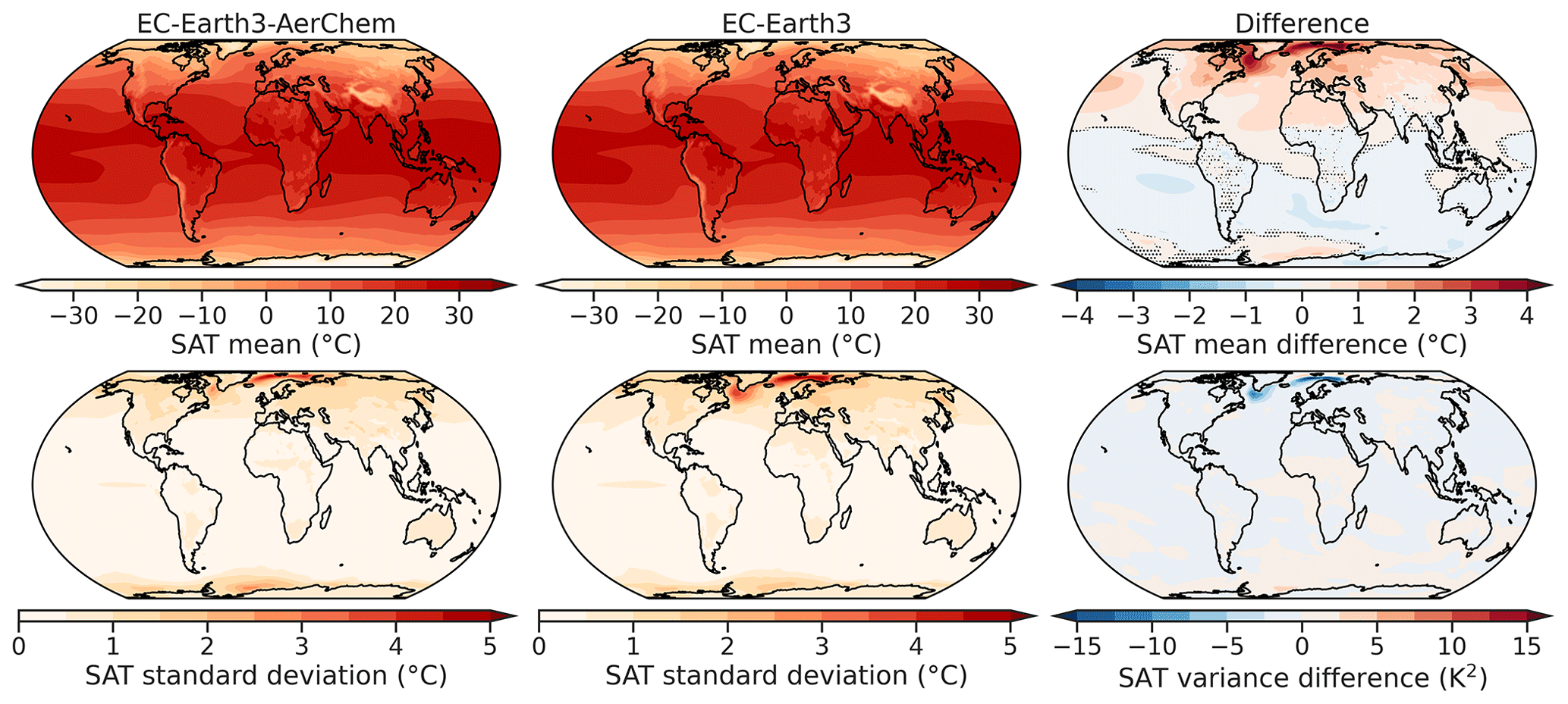
Figure 3 Mean and interannual standard deviation of the surface air temperature (SAT) in the Earth3-AerChem and EC-Earth3 preindustrial control simulation. The panels on the right show the corresponding differences in the mean and interannual variance in EC-Earth3-AerChem compared with EC-Earth3. The stippled areas in the top-right panel indicate the regions where the differences are not significant at the 5 % level, as determined from a two-sided unequal variances independent t test.

The higher mean temperatures over the Barents Sea, the Nordic Seas, and the Labrador Sea are associated with a strong reduction in interannual variability in these regions. In both simulations, there is a strong contribution from low-frequency variability in these areas (not shown). We have verified that a large part of the reduction in interannual variability in EC-Earth3-AerChem compared with EC-Earth3 in these regions is due to a reduction in interdecadal variability. In more northern parts of the Arctic Ocean, the interannual and interdecadal variability is somewhat enhanced in EC-Earth3-AerChem. This is also the case in most of the high-latitude regions of the Southern Ocean.

4.2 Climate sensitivity

In this section, we present estimates of the model's climate sensitivity obtained from the two DECK (Diagnostic, Evaluation and Characterization of Klima) CO₂ perturbation experiments. Figure 4a shows the time series of the annual mean GSAT change in these simulations relative to the unperturbed, preindustrial control simulation. Here, the preindustrial reference values are given by a linear fit through the corresponding 150-year section of piControl. By definition, the transient climate response (TCR) is calculated as the mean GSAT change in the experiment with atmospheric CO₂ concentrations increasing by 1 % yr⁻¹ (1pctCO2) over a 20-year period centered around the time of CO₂ doubling (i.e., simulation years 60–79; e.g., Meehl et al., 2020). This results in a TCR estimate of 2.1 ^∘C, which is slightly lower than the corresponding estimate of 2.3 ^∘C obtained for EC-Earth3 (from 1pctCO2 member r3i1p1f1) and in the middle of the range produced by CMIP6 models. For instance, Meehl et al. (2020) obtained a multi-model mean TCR of 2.0 ^∘C with a standard deviation of 0.4 ^∘C, based on CMIP6 model data available from the Earth System Grid Federation (ESGF) in March 2020.

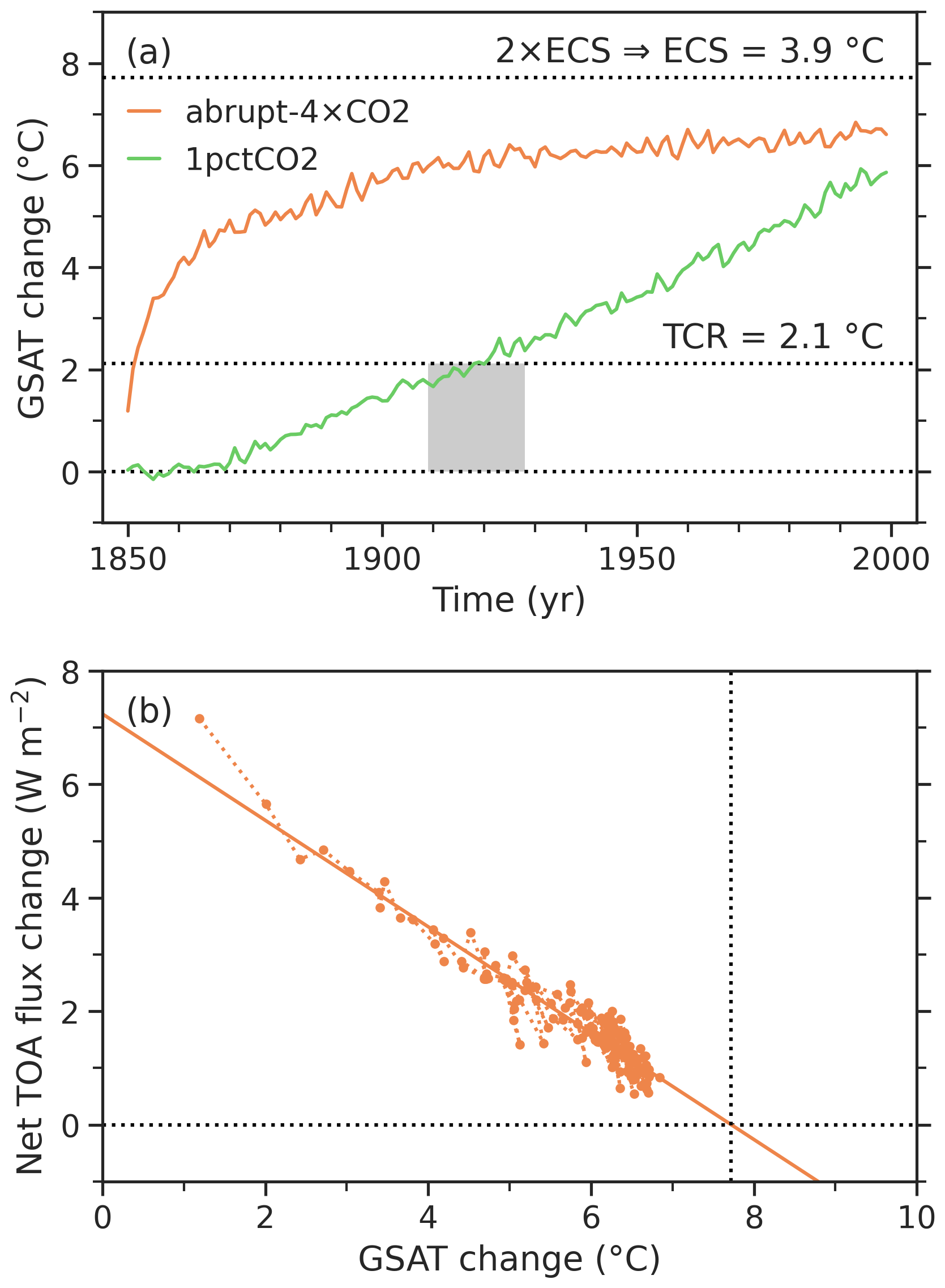
Figure 4 (a) GSAT change in the simulation with abrupt quadrupling of CO₂ concentrations (abrupt-4×CO2) and the simulation with a 1 % CO₂ concentration increase per year (1pctCO2). (b) Global net radiative flux change at the top of the atmosphere versus GSAT change in the abrupt-4×CO2 experiment, along with a linear fit obtained by Theil–Sen regression. The temperature and flux changes shown in this figure are the annual mean deviations from the linear trend lines through the corresponding 150 years of the preindustrial control simulation.

The model's effective climate sensitivity can be obtained from the experiment with quadrupled CO₂ concentrations (abrupt-4×CO2) by linearly regressing the annual mean net TOA flux change versus the annual mean GSAT change (Gregory et al., 2004; Andrews et al., 2012; Meehl et al., 2020; Sherwood et al., 2020), where a consistent definition of change is applied to both variables. Hence, the TOA flux change is corrected for the offset and drift in the corresponding section of the control simulation. Note that neither the TOA flux nor the global temperature shows a statistically significant drift in piControl over this 150-year period. The effective sensitivity is determined from the regression line as the GSAT change at the point where the net TOA flux change reaches zero, divided by 2.0 to convert to double CO₂. We have tested both ordinary least squares (OLS) regression and the Theil–Sen regression method, which is more robust to outliers, and applied these regression methods to the full 150-year period, as well as to restricted periods leaving out the first 5 (Wyser et al., 2020) or 20 years (e.g., Meehl et al., 2020). All methods produce a sensitivity estimate of 3.9 ^∘C. (OLS regression yields 3.86, 3.92, and 3.92 ^∘C for the 150-, 145-, and 130-year periods; the corresponding estimates from the Theil–Sen regression method are 3.86, 3.89, and 3.85 ^∘C.) As an example, Fig. 4b shows the linear fit obtained with Theil–Sen regression applied to the full 150-year period. The value of 3.9 ^∘C is close to the CMIP6 multi-model mean of 3.7 ^∘C from Meehl et al. (2020), but it is at the high end of the likely range estimated from multiple lines of evidence in the recent study by Sherwood et al. (2020). Applying the same regression methods to the EC-Earth3 abrupt-4×CO2 experiment (members r3i1p1f1 and r8i1p1f1) results in a sensitivity estimate of around 4.3 ^∘C. The lower estimate for EC-Earth3-AerChem is consistent with the reduction in TCR and in better agreement with the assessment by Sherwood et al. (2020).

4.3 Evaluation of surface air temperatures in the CMIP6 historical simulation

In this subsection, we present surface air temperatures from the four available realizations of the CMIP6 historical simulation and evaluate the results against observational data sets. The different ensemble members have been initialized from the preindustrial control simulation, using branching times 20 years apart. The first member (r1i1p1f1) was started from the initial state of piControl, and the second (r2i1p1f1), third (r3i1p1f1), and fourth (r4i1p1f1) members were started from the state obtained after 20, 40, and 60 years of piControl, respectively. We quantify the spread in the historical ensemble by the sample standard deviation across the individual members, denoted by σ.

Figure 5 shows the evolution of the annual mean GSAT in the four integrations, along with the corresponding ensemble median and mean values and the 1σ range around the mean. For comparison, the figure also shows the corresponding time series from the first 165 years of the preindustrial control simulation. The evolution of the global temperature during the 20th century differs strongly among the four members. Apart from short-term cooling events after large volcanic eruptions, the first, second, and fourth members remain relatively close to the preindustrial mean until about 1950. In contrast, the third member is in a significantly colder state during most of the 20th century. In this period, the spread among the four members exceeds the range of internal variability displayed by the preindustrial simulation. The ensemble median is higher than the mean for most years in the period from 1920 to 1960. In the earlier and later periods, the differences between the median and mean are small. The mean GSAT in the final 10 years of the historical simulation (2005–2014) is 14.76 ± 0.03 (σ =0.19) ^∘C. This is ∼ 0.7 ^∘C above the preindustrial mean.

Figure 5 Time series of the annual and global mean surface air temperature for the four realizations of the CMIP6 historical simulation (a), and the corresponding ensemble median and mean values (b). In both panels, the gray area indicates the range bounded by 1 standard deviation around the ensemble mean, and the dotted line indicates the preindustrial mean of 14.08 ^∘C. For comparison, panel (a) also shows the corresponding time series for the first 165 years of the preindustrial control simulation.

In Fig. 6, the median, mean, and 1σ range of annual temperature anomalies are compared against the GISS Surface Temperature Analysis (GISTEMP) version 4 (Lenssen et al., 2019; GISTEMP Team, 2020) and version 2.0 of the temperature reconstruction by Cowtan and Way (2014, 2021). Both data sets combine SAT anomalies over land and sea ice with SST anomalies over open sea. Whereas surface air and water temperatures may be very different, their anomalies are very similar over open sea. Therefore, we can directly compare the SAT anomalies simulated by the model with the reconstructed anomalies. A more robust comparison would use a blend of air and water temperatures also from the model (Cowtan et al., 2015), but such an analysis is beyond the scope of this paper. The anomalies shown in the figure are calculated with respect to the 1850–1900 period or, for GISTEMP, the 1880–1900 period. The simulated mean GSAT in this period is 14.15 ± 0.01 (σ =0.08) ^∘C.

Figure 6 The median, mean, and 1 standard deviation range of the annual mean surface air temperature (SAT) anomalies from the four realizations of the CMIP6 historical simulation compared with reconstructed surface temperature anomalies from GISTEMP version 4 and HadCRUT4 infilled by kriging (Cowtan and Way version 2.0). The anomalies are defined with respect to the 1850–1900 period (1880–1900 for GISTEMP). Panels (a), (b), and (c) show the global, Northern Hemisphere, and Southern Hemisphere means, respectively.

Figure 6a shows that the ensemble of four realizations tends to underestimate the observed global temperature anomalies from the end of the 19th century onwards. The upper end of the 1σ range follows the observational time series reasonably well until the middle of the 20th century. In contrast to the observations, the warmer members show a substantial global cooling during the 1950s and 1960s (see Fig. 5), partly caused by the eruption of Mount Agung in 1963. As a result, all members produce negative anomalies from the 1960s to the end of the 1980s, whereas the observed anomalies remain positive during these years. In the final decades of the historical period, the simulations tend to overestimate the observed warming trend. The mean GSAT anomaly for the years 2005–2014 is 0.62 ± 0.04 (σ =0.23) ^∘C. For this period, the GISTEMP and Cowtan and Way time series give a global warming of 0.87 ± 0.02 and 0.89 ± 0.02 ^∘C, respectively. As can be seen in Fig. 6b and c, the spread among ensemble members as well as the discrepancies with the observed time series are almost entirely caused by variability in Northern Hemisphere temperatures. The simulated temperature anomalies for the Southern Hemisphere agree rather well with the observed time series. For the SH, the ensemble mean for the 2005–2014 period is 0.69 ± 0.02 (σ =0.04) ^∘C, compared with 0.65 ± 0.02 ^∘C in GISTEMP and 0.68 ± 0.02 ^∘C in the Cowtan and Way reconstruction.

We have verified that the climate states characterized by anomalously low temperatures in the NH are associated with periods of reduced convective mixing in the Labrador Sea. This suggests that the interdecadal variability in the historical simulation is enhanced by the same instability mechanism that introduces long-term variations in the preindustrial simulation. Other EC-Earth3 configurations also produce spurious interdecadal variability in preindustrial and historical simulations (Döscher et al., 2021; Parsons et al., 2020), and we believe that the underlying mechanism is similar.

Next, we evaluate the ensemble mean SAT climatology for the last 20 years of the historical simulation (1995–2014) using the ERA5 reanalysis from the ECMWF (Hersbach et al., 2020; Copernicus Climate Change Service, 2017) as the observational reference. In Fig. 7, we compare the climatological SAT distributions for all seasons, and for boreal winter (December, January, and February) and summer (June, July, and August) separately. The ensemble mean GSAT bias with respect to ERA5 for this period is 0.22 ± 0.03 (σ =0.18) ^∘C. The mean SAT bias is 1.29 ± 0.02 (σ =0.05) ^∘C in the Southern Hemisphere and −0.86 ± 0.05 (σ =0.35) ^∘C in the Northern Hemisphere.

The strongest biases are observed over the Southern Ocean and Antarctica, where temperatures are overestimated throughout the year. Near the coast of Antarctica, annual biases of up to 12.5 ^∘C are found. Warm biases also exist in the subtropical marine stratocumulus regions in the eastern South Atlantic and the eastern North and South Pacific. These biases are common to many climate models and have been attributed to biases in SW cloud radiative effects (Bodas-Salcedo et al., 2014, 2016; Calisto et al., 2014; Forbes and Ahlgrimm, 2014; Hogan et al., 2017). Temperatures are also overestimated over the Gulf of Alaska and the Bering Sea. Moreover, a warm bias is found in the Kazakhstan region, mostly during winter. The model underestimates the seasonal cycle in northeastern Siberia, resulting in a warm bias during winter and a cold bias during summer. Strong cold biases exist during winter over the Arctic Ocean, the Labrador Sea, and the North Atlantic as well as in the Middle East, northern Africa, and the United States. As the NH is warming faster than observed, most of these cold biases tend to be reduced when moving towards the end of the historical period. For instance, restricting the comparison to the final 10 years of the simulation (2005–2014) reduces the mean bias in the NH to −0.68 ± 0.06 (σ =0.37) ^∘C.

Figure 7 Surface air temperature (SAT) climatology for the years 1995–2014 from the four-member ensemble of the CMIP6 historical simulation and the ERA5 reanalysis (version 2), and the corresponding differences. The top row shows the full multiannual means, and the middle and bottom rows show the means for boreal winter (December, January, February; DJF) and summer (June, July, August; JJA), respectively. The number given in the top right of each panel is the global mean value. The stippled areas in the panels on the right indicate the regions where the differences are not significant at the 5 % level, as determined from a two-sided unequal variances independent t test.

In Fig. 8, we compare the ensemble median, mean, and 1σ range of the zonal annual mean SAT bias as a function of latitude for the years 1995–2014 and 1850–1900, respectively. The observational reference for the 1850–1900 period was estimated from the 1995–2014 mean SAT fields from ERA5 reduced by the warming between the two periods, calculated from the anomaly fields from the Cowtan and Way reconstruction. For the early period, the figure also shows the zonal mean difference between the 500-year means from the EC-Earth3-AerChem and EC-Earth3 preindustrial control simulations, respectively, and the observational estimate. Note that, for EC-Earth3-AerChem, the preindustrial mean almost coincides with the median of the historical ensemble for 1850–1900. Zonal biases are positive at latitudes south of ∼ 20^∘ S. These biases are quantitatively similar in the two periods, indicating that the warming at these latitudes is well reproduced by the model. At latitudes north of ∼ 20^∘ S, the warming is underestimated. Here, the ensemble median and mean zonal bias for 1995–2014 is negative at all latitudes, whereas the zonal bias for 1850–1900 oscillates around zero as a function of latitude.

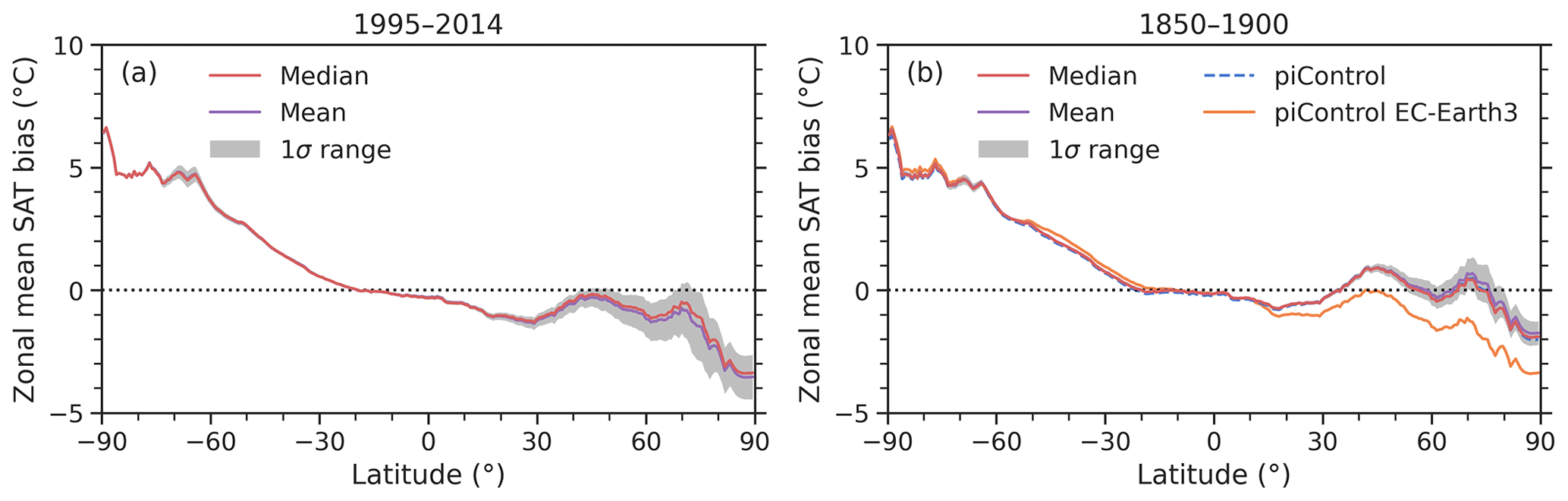
Figure 8 Zonal mean surface air temperature (SAT) bias as a function of latitude for the years 1995–2014 (a) and 1850–1900 (b). In panel (a), the bias is calculated with respect to the ERA5 reanalysis; to calculate the bias for the early historical period displayed in panel (b), the 1995–2014 mean SAT fields from ERA5 have been reduced by the warming between the two periods, estimated from the temperature anomaly fields from HadCRUT4 infilled by kriging (Cowtan and Way version 2.0). Both panels show the median, mean, and 1 standard deviation range of the bias from the four realizations of the CMIP6 historical simulation. For comparison, panel (b) also shows the deviation of the 500-year mean from the preindustrial control simulation from the observational estimate for 1850–1900, for both EC-Earth3-AerChem and EC-Earth3.

4.4 Historical and future perturbation experiments

In this subsection, we present the evolution of the global surface air temperature, the global net TOA flux, and tropospheric aerosol optical depth (AOD) from 1850 to 2100 for various CMIP6 and AerChemMIP experiments. Except for the temperature evolution in the CMIP6 historical simulation, the results are taken from a single realization of these experiments (member r1i1p1f1). Figure 9 shows the annual mean temperature and flux perturbations for the different experiments relative to the preindustrial means given in Sect. 4.1. The corresponding time series of the annual global mean tropospheric aerosol optical depth (AOD) at 550 nm are presented in Fig. 10. For the historical period, the CMIP6 historical simulation is compared with the AerChemMIP hist-piNTCF and hist-piAer experiments. In hist-piNTCF, the emissions of near-term climate forcers (NTCFs) are kept at preindustrial levels. NTCFs include aerosols and precursors of aerosols and ozone. The ozone precursors comprise NO_x, CO, and NMVOCs. Although methane is an ozone precursor, it is not included in the AerChemMIP definition of NTCFs. In hist-piAer, only the emissions of aerosols (BC and OA) and aerosol precursors (SO_x and NH₃) are kept at preindustrial levels.

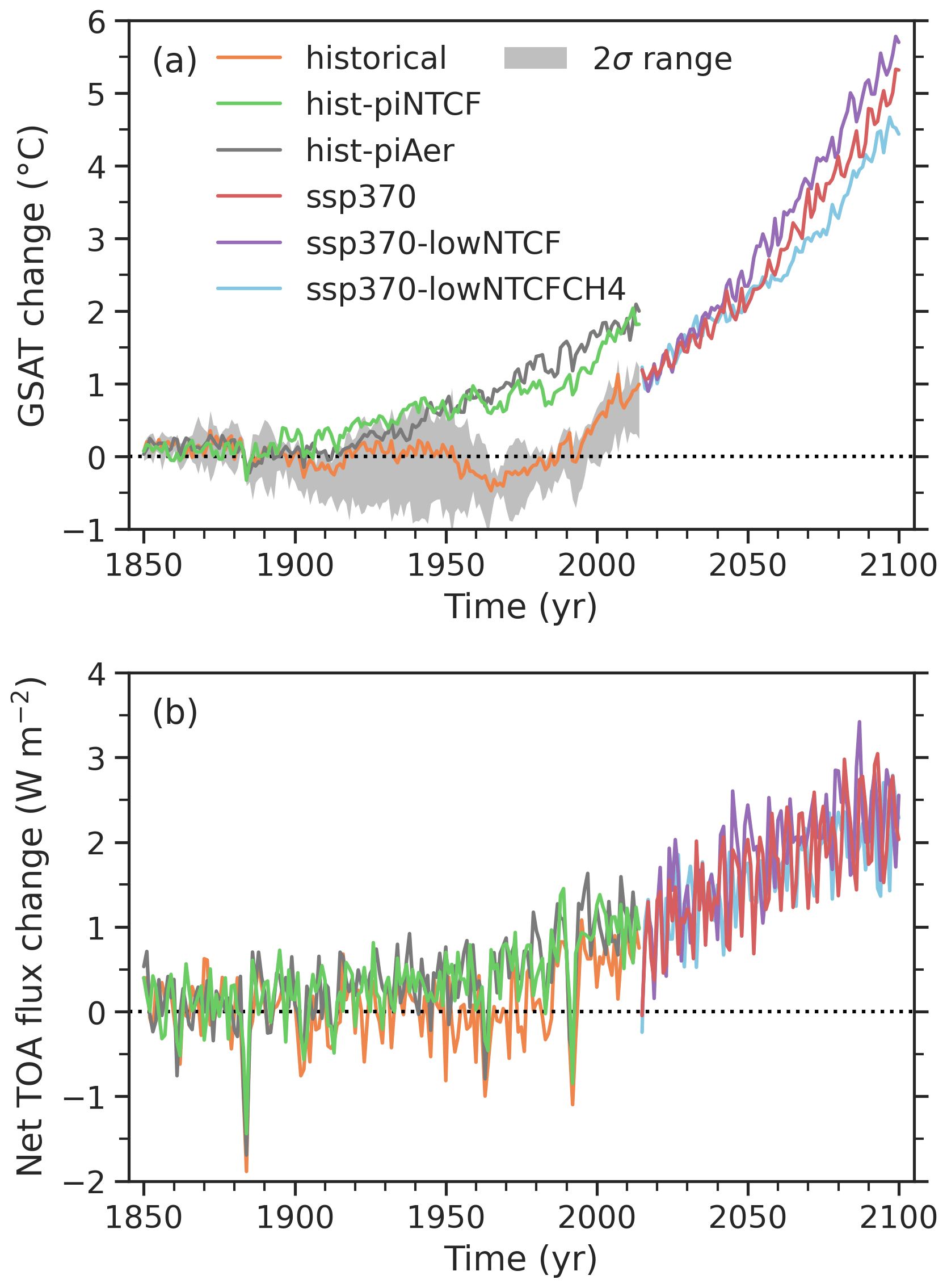
Figure 9 Change in (a) the global surface air temperature (GSAT) and (b) the global net TOA flux in the CMIP6 historical simulation, the AerChemMIP historical perturbation experiments hist-piNTCF and hist-piAer, and future simulations for the standard SSP3-7.0 scenario, a corresponding scenario with low NTCF emissions (SSP3-7.0-lowNTCF), and a corresponding scenario with both low NTCF emissions and low CH₄ concentrations (SSP3-7.0-lowNTCFCH4). The temperature and flux changes shown in this figure are the annual mean deviations from the preindustrial means given in Fig. 2a and c, respectively. Only the first ensemble member (r1i1p1f1) of each experiment is presented; for the GSAT change in the CMIP6 historical simulation, the range bounded by 2 standard deviations around the mean of the four-member ensemble is also shown.

The global mean tropospheric AOD at 550 nm is 0.094 with an interannual standard deviation of 0.003 in the preindustrial control simulation and increases to on average 0.135 ± 0.001 by the end of the historical simulation (2005–2014). The hist-piNTCF and hist-piAer experiments yield higher global temperatures than the corresponding member of the standard historical simulation from the early 20th century onwards. However, the standard historical simulation for this period displays a large spread across ensemble members, and the differences with the perturbation experiments in the first half of the century may not be statistically significant. From around 1950 onwards, global temperatures in the two perturbation experiments are systematically above the 2σ range of the four members of the historical simulation. The maximum 10-year rolling mean difference compared with the historical ensemble is 1.19 ± 0.04 (σ =0.17) ^∘C for hist-piNTCF attained in the years 1972–1981 and 1.49 ± 0.06 (σ =0.15) ^∘C for hist-piAer in 1990–1999. At the end of the historical period (2005–2014) these differences have been reduced to 1.12 ± 0.05 and 1.16 ± 0.06 ^∘C, respectively, with σ=0.19 ^∘C. A more quantitative analysis of the impact of aerosol and ozone precursor emissions in the historical period requires ensemble simulations, which are in production. The time series of the TOA fluxes show large interannual variability with strong downward excursions after major volcanic eruptions, reaching a mean value at the end of the historical period (2005–2014) of 0.62 ± 0.09 W m⁻² in the historical simulation member and 0.91 ± 0.08 and 0.96 ± 0.09 W m⁻² in the hist-piNTCF and hist-piAer experiments, respectively.

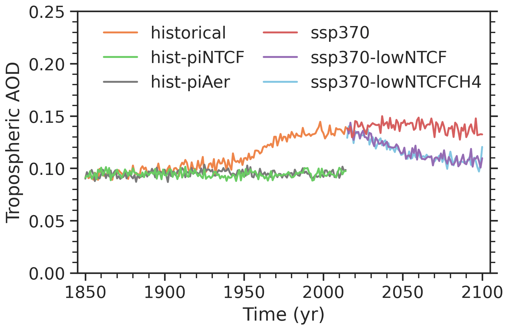
Figure 10 Annual global mean tropospheric aerosols optical depth (AOD) at 550 nm in the simulations presented in Fig. 9.

Projections are given for three scenarios, which only differ with respect to assumptions regarding NTCF emissions and methane concentrations. The first scenario experiment (ssp370) follows the standard SSP3-7.0 from ScenarioMIP (O'Neill et al., 2016), which has relatively high emissions of NTCFs (Gidden et al., 2019). For this scenario, EC-Earth3-AerChem produces a global warming of 4.9 ^∘C towards the end of the century (2091–2100). The second is the AerChemMIP experiment ssp370-lowNTCF, which follows the same Shared Socioeconomic Pathway but with reduced emissions of NTCFs (Gidden et al., 2019). This scenario produces enhanced warming, reaching 5.4 ^∘C in the final decade. Finally, in ssp370-lowNTCFCH4, it is assumed that both NTCF emissions and CH₄ concentrations will be reduced compared to ssp370. This scenario produces a significantly lower warming of 4.4 ^∘C. Thus, for these scenarios, reductions in CH₄ concentrations more than offset the enhanced warming due to reductions in NTCF emissions. A more detailed multi-model analysis for these scenario experiments is presented in Allen et al. (2020).

5 Discussion and conclusions

This paper documents the global climate model EC-Earth3-AerChem. EC-Earth3-AerChem is a configuration of the EC-Earth3 family of models with interactive tropospheric aerosols and atmospheric chemistry. It uses a coupling between an IFS-based atmospheric GCM and the TM5 atmospheric chemistry and transport model to simulate aerosol–radiation and aerosol–cloud interactions as well as chemistry–climate interactions and radiative effects of ozone and methane. We have described the model with a focus on the specific features of EC-Earth3-AerChem compared with the other EC-Earth3 configurations (Döscher et al., 2021), and on the updates and improvements introduced in TM5 and the TM5–IFS coupled system since the publication of EC-Earth 2.4 (van Noije et al., 2014).

The model's preindustrial climate was analyzed from a 500-year-long preindustrial control experiment (piControl). The global surface air temperature (GSAT) in this simulation is on average 14.08 ^∘C with an interannual standard deviation of 0.17 ^∘C, and it exhibits a small linear trend of 0.015 ± 0.005 ^∘C per century. The global net TOA energy imbalance is only −0.09 ± 0.25 W m⁻² and shows no statistically significant drift. The model displays substantial low-frequency variability on interdecadal to centennial timescales, with a clear correlation between the long-term evolution of GSAT and the strength of the Atlantic meridional overturning circulation (AMOC), which is in turn driven by deep-water formation in the Labrador Sea.

Compared with the standard EC-Earth3 configuration (piControl member r1i1p1f1), the preindustrial climate of EC-Earth3-AerChem is characterized by a substantially warmer Northern Hemisphere (0.61 ± 0.02 ^∘C) and a slightly colder Southern Hemisphere (−0.18 ± 0.01 ^∘C), in agreement with observational estimates of 19th century temperatures. Moreover, EC-Earth3-AerChem exhibits lower internal variability and a lower correlation between the global temperature and the strength of the AMOC. The largest temperature differences are found over the Barents Sea, the Nordic Seas, and the Labrador Sea, where substantially higher temperatures in EC-Earth3-AerChem are associated with a strong reduction in interannual and interdecadal variability.

The differences between the preindustrial climates of EC-Earth3-AerChem and EC-Earth3 are due to a combination of the effects of the different representation of aerosols and atmospheric chemistry and a subsequent retuning of the model involving three parameters in the IFS model. As described in Sect. 3, switching to interactive aerosols and chemistry had a substantial impact on the model's climate, especially in the NH high-latitude regions where surface air temperatures increased substantially. This is mostly the result of the interactive nature of the aerosols in EC-Earth3-AerChem. For high-latitude ocean regions, one can imagine that interactions between aerosols, clouds, and sea ice are of particular importance, but we have not analyzed this in detail.

The model's effective equilibrium climate sensitivity (ECS) was robustly estimated at 3.9 ^∘C, using 130 to 150 years of an abrupt-4×CO2 experiment. This is close to the CMIP6 multi-model mean of 3.7 ^∘C presented by Meehl et al. (2020) but at the high end of the likely range estimated in the recent study by Sherwood et al. (2020). Similarly, the model's transient climate response (TCR) was calculated from a 1pctCO2 experiment, resulting in a value of 2.1 ^∘C. Again, this is close to the CMIP6 multi-model mean of 2.0 ^∘C from Meehl et al. (2020).

A four-member ensemble of the CMIP6 historical simulation shows large interdecadal variability in Northern Hemisphere and global temperatures during the 20th century, resulting in a large spread among the different members. The mean GSAT in the last decade of the simulation (2005–2014) is 14.76 ± 0.03 (σ =0.19) ^∘C, which is ∼ 0.7 ^∘C above the preindustrial mean. Here, the standard deviation σ indicates the spread across the ensemble members.

The evolution of annual mean surface air temperature (SAT) anomalies in the historical ensemble has been compared with observational time series from Cowtan and Way (version 2.0) and GISTEMP (version 4). The model underestimates the warming over the historical period. The mean temperature change between the second half of the 19th century (1850–1900) and the 2005–2014 period is 0.62 ± 0.04 (σ =0.23) ^∘C in the simulations compared with 0.87 and 0.89 ± 0.02 ^∘C in the GISTEMP and Cowtan and Way data sets, respectively. The observed warming of the Southern Hemisphere is well reproduced by the model. For the SH, the mean SAT anomaly for the 2005–2014 period is 0.69 ± 0.02 (σ =0.04) ^∘C, compared with 0.65 and 0.68 ± 0.02 ^∘C in the reconstructions.

At least part of the spurious interdecadal variability in our simulations is related to the intermittent nature of the convection in the Labrador Sea, where a reduction or shutdown of the convection during extended periods of time causes a weakening of the AMOC and anomalously low temperatures in the Northern Hemisphere. Other EC-Earth3 configurations also display spurious interdecadal variability in preindustrial and historical simulations (Döscher et al., 2021), and we believe the underlying mechanism is similar and is related to the use of NEMO3.6 and the relatively coarse resolution of the ORCA1 grid. It is known that the resolution of the ocean model is a critical factor for deep-water formation in the Labrador Sea. For instance, in the study by Koenigk et al. (2020), increasing the ocean resolution from ORCA1 to ORCA025 resulted in increased deep convection in the Labrador Sea in four out of the five models that use NEMO3.6 (HadGEM3-GC31, CMCC-CM2, CNRM-CM6-1, and EC-Earth3P). Moreover, Parsons et al. (2020) examined interdecadal GSAT variability in preindustrial control simulations from 39 CMIP6 models. The six models showing the largest variability are EC-Earth3, BCC-CSM2-MR, CNRM-ESM2-1, EC-Earth3-Veg, CNRM-CM6-1, and IPSL-CM6A-LR. Five of these use NEMO3.6 on the ORCA1 grid (EC-Earth3 and EC-Earth3-Veg) or extended ORCA1 (eORCA1) grid (CNRM-ESM2-1, CNRM-CM6-1, and IPSL-CM6A-LR). The mechanism underlying the multicentennial variability in IPSL-CM6A-LR has recently been investigated by Jiang et al. (2021) and has been shown to be associated with freshwater accumulation and release in the Arctic, modulated by the interplay between sea ice and oceanic freshwater export from the Arctic. The EC-Earth consortium has recently started a detailed investigation of the mechanism responsible for the long-term oscillations in the EC-Earth3 model.

We do not want to suggest that the use of NEMO3.6 on the ORCA1 grid will produce similar behavior irrespective of the details of the NEMO configuration or other model components. Studies with EC-Earth3 indicate that phases characterized by a weakening of the AMOC correspond to extended periods with reduced convective activity and high sea-ice coverage in the Labrador Sea (Döscher et al., 2021). As these processes are state dependent, the choice of ocean parameters or atmospheric model can have a strong impact on the simulated convection (Koenigk et al., 2020). For future research, it would be interesting to consider increasing the resolution of the ocean model in EC-Earth3-AerChem.

The model simulates a cooling of the Northern Hemisphere in the 1950s and 1960s. This likely is related to aerosols and suggests that the model overestimates the aerosol forcing in this period. Simulations that provide more information on the role of aerosols and their effective radiative forcing contributions are in production.

The ensemble mean SAT climatology for the years 1995–2014 has been evaluated against the ERA5 reanalysis from the ECMWF. The GSAT bias for this period is 0.22 ± 0.03 (σ =0.18) ^∘C. The mean SAT bias is 1.29 ± 0.02 (σ =0.05) ^∘C in the SH and $-\mathrm{0.86}\pm \mathrm{0.05}$ (σ =0.35) ^∘C in the NH. As the ensemble overestimates the NH warming trends during this period, cold biases in the NH tend to be reduced towards the end of the simulation. For instance, for the last 10 years of the simulation (2005–2014), the mean NH cold bias is reduced to 0.68 ± 0.06 (σ =0.37) ^∘C.

Over the Southern Ocean and Antarctica strong warm biases are found in all seasons. Temperatures are also overestimated in subtropical marine stratocumulus regions. These biases are common to many climate models, including all EC-Earth3 configurations, and have been attributed to biases in SW cloud radiative effects. Modifications in the cloud scheme and the representation of supercooled liquid water made in more recent versions of IFS, including cycle 45r1 (Forbes and Ahlgrimm, 2014; Forbes et al., 2016), along with the introduction of the new ecRad radiation scheme in cycle 43r3 (Hogan et al., 2017) have been shown to substantially reduce these biases.

To illustrate the applicability of the model, time series of the GSAT and net TOA flux change relative to their preindustrial levels have been presented for a number of historical and scenario perturbation experiments from AerChemMIP. For the historical period, two perturbation experiments have been considered: hist-piNTCF, in which emissions of near-term climate forcers (NTCFs) are fixed to preindustrial levels, and hist-piAer, which uses preindustrial emissions only for aerosols and aerosol precursors. Both experiments produce significantly higher temperatures than the standard historical simulation from the second half of the 20th century onwards. For the future period, the standard SSP3-7.0 Shared Socioeconomic Pathway from ScenarioMIP has been compared with a scenario with lower NTCF emissions (SSP3-7.0-lowNTCF) and one with both lower NTCF emissions and lower methane concentrations (SSP3-7.0-lowNTCFCH4). For SSP3-7.0, the model projects a global warming at the end of the century (2091–2100) of about 4.9 ^∘C above the preindustrial level. For the scenario with reduced NTCFs, the warming is increased by about 0.5 ^∘C, whereas for the scenario with both NTCFs and methane reduced, the warming is decreased by about 0.5 ^∘C. Note that these estimates are based on a single realization of each experiment. Ensembles required to reduce the impact of internal variability are in production.

The representation of aerosols and chemistry has been updated in numerous respects compared with the model version presented by van Noije et al. (2014). The overall result of these changes is a much improved description of, in particular, aerosol concentrations and optical properties (Bergman et al., 2021; Gliß et al., 2021; Checa-Garcia et al., 2021). One highlight worth mentioning is that EC-Earth3-AerChem produces substantially higher and more realistic aerosol optical depths (AOD). The global mean tropospheric AOD at 550 nm increases from 0.094 with an interannual standard deviation of 0.003 in the preindustrial control simulation to on average 0.135 ± 0.001 in the last decade of the historical simulation (2005–2014). The study by Gliß et al. (2021) provides numbers for the global annual emissions of primary aerosols and the global burdens and atmospheric lifetimes of various aerosol components in a nudged atmosphere-only simulation for the year 2010. A detailed evaluation of the aerosol simulation by the model is beyond the scope of this paper.

The increased complexity from interactive aerosols and atmospheric chemistry comes at the expense of computational performance. The single-core OASIS transfer of spectral fields from IFS to TM5 has been identified as a major bottleneck limiting the scalability of the model. It is expected that a substantial speedup can be achieved by converting the spectral fields to grid-point fields at the IFS side, enabling domain decomposition and multicore transfer to TM5. This is planned as part of the model's near-term development. A parallel development is the integration of aerosol and chemistry modules into the OpenIFS model, which will be the atmospheric GCM in the next generation of EC-Earth (e.g., Kjellsson et al., 2020).

Meanwhile, a number of developments aiming to improve the representation of aerosol and chemical processes are underway. These include the replacement of EQSAM with ISORROPIA II (Fountoukis and Nenes, 2007) or a light version thereof, which is expected to improve the calculation of aerosol water and acidity, as well as the inclusion of coarse-mode nitrate. The MOGUNTIA gas-phase chemistry mechanism has recently been introduced as a more explicit alternative to the current scheme based on CB05 (Myriokefalitakis et al., 2020). A parameterization of marine organic aerosol emissions is also available. Other developments aim to improve the representation of the mineralogical composition and size distribution of dust (Perlwitz et al., 2015a, b; Pérez García-Pando et al., 2016; Adebiyi and Kok, 2020) along with the associated effects upon radiation and clouds. Furthermore, it is envisaged that the aerosol activation scheme from Abdul-Razzak and Ghan (2000) will be replaced by the more accurate parameterization developed by Morales Betancourt and Nenes (2014), using a more sophisticated turbulence-dependent calculation of the updraft velocity.