the Creative Commons Attribution 4.0 License.
the Creative Commons Attribution 4.0 License.
 | 13 Sep 2021
Combining ensemble Kalman filter and reservoir computing to predict spatiotemporal chaotic systems from imperfect observations and models
Futo Tomizawa
Yohei Sawada
Prediction of spatiotemporal chaotic systems is important in various fields, such as numerical weather prediction (NWP). While data assimilation methods have been applied in NWP, machine learning techniques, such as reservoir computing (RC), have recently been recognized as promising tools to predict spatiotemporal chaotic systems. However, the sensitivity of the skill of the machine-learning-based prediction to the imperfectness of observations is unclear. In this study, we evaluate the skill of RC with noisy and sparsely distributed observations. We intensively compare the performances of RC and local ensemble transform Kalman filter (LETKF) by applying them to the prediction of the Lorenz 96 system. In order to increase the scalability to larger systems, we applied a parallelized RC framework. Although RC can successfully predict the Lorenz 96 system if the system is perfectly observed, we find that RC is vulnerable to observation sparsity compared with LETKF. To overcome this limitation of RC, we propose to combine LETKF and RC. In our proposed method, the system is predicted by RC that learned the analysis time series estimated by LETKF. Our proposed method can successfully predict the Lorenz 96 system using noisy and sparsely distributed observations. Most importantly, our method can predict better than LETKF when the process-based model is imperfect.
- Article
(2564 KB) - Full-text XML
- BibTeX
- EndNote


In numerical weather prediction (NWP), it is required to obtain the optimal estimation of atmospheric state variables using observations and process-based models, which are both imperfect. Observations of atmospheric states are sparse and noisy, and numerical models inevitably include biases. In addition, models used in NWP are known to be chaotic, which makes the prediction substantially difficult. To accurately predict the future atmospheric state, it is important to develop methods to predict spatiotemporal chaotic dynamical systems from imperfect observations and models.
Traditionally, data assimilation methods have been widely used in geosciences and NWP systems. Data assimilation is a generic term for approaches to estimate the state from observations and model outputs based on their errors. The state estimated by data assimilation is used as the initial value, and the future state is predicted by models alone. Data assimilation is currently adopted in operational NWP systems. Many data assimilation frameworks have been proposed, e.g., 4D variational methods (4D-Var; Bannister, 2017), ensemble Kalman filter (EnKF; Houtekamer and Zhang, 2016), or their derivatives, and they have been applied to many kinds of weather prediction tasks, such as the prediction of short-term rainfall events (e.g., Sawada et al., 2019; Yokota et al., 2018) and severe storms (e.g., Zhang et al., 2016). Although data assimilation can efficiently estimate the unobservable state variables from noisy observations, the prediction skill is degraded if the model has large biases. On the other hand, model-free prediction methods based on machine learning have received much attention recently. In the context of dynamical system theory, previous works have developed methods to reproduce the dynamics by inferring it purely from observation data (Rajendra and Brahmajirao, 2020), or by combining a data-driven approach and physical knowledge on the systems (Karniadakis et al., 2021). In the NWP context, many previous studies have successfully applied machine learning to predict chaotic dynamics. Vlachas et al. (2018) successfully applied long short-term memory (LSTM; Hochreiter and Schmidhuber, 1997) to predict the dynamics of the Lorenz96 model, Kuramoto–Sivashinski Equation, and the barotropic climate model which is a simple atmospheric circulation model. Asanjan et al. (2018) showed that LSTM can accurately predict the future precipitation by learning satellite observation data. Nguyen and Bae (2020) successfully applied LSTM to generate area-averaged precipitation prediction for hydrological forecasting.
In addition to LSTM, reservoir computing (RC), which was first introduced by Jaeger and Haas (2004), has been found to be suitable to predict spatiotemporal chaotic systems. Pathak et al. (2017) successfully applied RC to predict the dynamics of Lorenz equation and Kuramoto–Sivashinski equation. Lu et al. (2017) showed that RC can be used to estimate state variables from sparse observations if the whole system was perfectly observed as training data. Pathak et al. (2018b) succeeded in using a parallelized RC to predict each segment of the state space locally, which enhanced the scalability of RC to much higher dimensional systems. Chattopadhyay et al. (2020) revealed that RC can predict the dynamics of the Lorenz 96 model more accurately than LSTM and artificial neural networks (ANNs). In addition to the accuracy, RC also has an advantage in computational costs. RC can learn the dynamics only by training a single matrix as a linear minimization problem just once, while other neural networks have to train numerous parameters and need many iterations (Lu et al., 2017). Thanks to this feature, the computational costs needed to train RC are lower than those of LSTM and ANN.
However, Vlachas et al. (2020) revealed that the prediction accuracy of RC is degraded when all of the state variables cannot be observed. It can be a serious problem since the observation sparsity is often the case in geosciences and the NWP systems. Brajard et al. (2020) pointed out this issue and successfully trained the convolutional neural network (CNN) with sparse observations, by combining it with EnKF. However, their method needs to iterate the data assimilation and training until the prediction accuracy of the trained model converges. Although one can stop the iteration after a few time steps, training can be computationally expensive if one waits for convergence. Bocquet et al. (2020) proposed a method to combine EnKF and machine learning methods to obtain both the state estimation and the surrogate model online. They showed successful results without using the process-based model at all. Dueben and Bauer (2018) mentioned that the spatiotemporal heterogeneity of observation data made it difficult to train machine learning models, and they suggested using the model or reanalysis as training data. Weyn et al. (2019) successfully trained machine learning models using the atmospheric reanalysis data.
We aim to propose the novel methodology to predict spatiotemporal chaotic systems from imperfect observations and models. First, we reveal the limitation of the standalone use of RC under realistic situations (i.e., imperfect observations and models). Then, we propose a new method to maximize the potential of RC to predict chaotic systems from imperfect models and observations, which is even computationally feasible. As Dueben and Bauer (2018) proposed, we make RC learn the analysis data series generated by a data assimilation method. Our new method can accurately predict from imperfect observations. Most importantly, we found that our proposed method is more robust to model biases than the standalone use of data assimilation methods.
2.1 Lorenz 96 model and OSSE
We used a low-dimensional spatiotemporal chaotic model, the Lorenz 96 model (L96), to perform experiments with various parameter settings. L96 is a model introduced by Lorenz and Emanuel (1998) and has been commonly used in data assimilation studies (e.g., Kotsuki et al., 2017; Miyoshi, 2005; Penny, 2014; Raboudi et al., 2018). L96 is recognized as a good test bed for the operational NWP problems (Penny, 2014).
In this model, we consider a ring-structured and m-dimensional discrete state space (that is, xm is adjacent to x1) and define the system dynamics as follows:
where F stands for the force parameter, and we define , x0=xm, and . Each term of this equation corresponds to advection, damping, and forcing respectively. It is known that the model with m=40 and F=8 shows chaotic dynamics with 13 positive Lyapunov exponents (Lorenz and Emanuel, 1998), and this setting is commonly used in the previous studies (e.g., Kotsuki et al., 2017; Miyoshi, 2005; Penny, 2014; Raboudi et al., 2018). The time width Δt=0.2 corresponds to one day in real atmospheric motion from the view of dissipative decay time (Lorenz and Emanuel, 1998).
As we use this conceptual model, we cannot obtain any observational data or “true” phenomena that correspond to the model. Instead, we adopted an observing system simulation experiment (OSSE). We first prepared a time series by integrating Eq. (1) and regarded it as the “true” dynamics (called Nature Run). Observation data can be calculated from this time series by adding some perturbation:
where yo∈ℝh is the observation value, H is the m×h observation matrix, and ϵ∈ℝh is the observational error whose each element is independent and identically distributed from a Gaussian distribution N(0,e) for observation error e.
In each experiment, the form of L96 used to generate Nature Run is unknown, and the model used to make predictions can be different from that for Nature Run. The difference between the model used for Nature Run and that used for prediction corresponds to the model's bias in the context of NWP.
2.2 Local ensemble transform Kalman filter
We used the local ensemble transform Kalman filter (LETKF, Hunt et al., 2007) as the data assimilation method in this study. LETKF is one of the ensemble-based data assimilation methods, which is considered to be applicable to the NWP problems in many previous studies (Sawada et al., 2019; Yokota et al., 2018). LETKF is also used for the operational NWP in some countries (e.g., Germany; Schraff et al., 2016).
LETKF and the family of ensemble Kalman filters have two steps: forecast and analysis. The analysis step makes the state estimation based on the forecast variables and observations. The forecast step makes the prediction from the current analysis variables to the time for the next analysis using the model. The interval for each analysis is called the “assimilation window”.
Considering the stochastic error in the model, system dynamics can be represented as follows (hereafter the subscript k stands for the variable at time k, and the time width between k and k+1 corresponds to the assimilation window):
where denotes the forecast variables, denotes the analysis variables, is the model dynamics operator, η∈ℝm is the stochastic error, and N(0,Q) means the multivariate Gaussian distribution with mean 0 and n×n covariance matrix Q. Since the error in the model is assumed to follow the Gaussian distribution, forecasted state xf can also be considered as a random variable from the Gaussian distribution. When the assimilation window is short, the Gaussian nature of the forecast variables is preserved even if the model dynamics is nonlinear. In this situation, the probability distribution of xf (and also xa) can be parametrized by mean and covariance matrix Pf ().
Using the computed state vector , observation variables can be estimated as follows:
where yf∈ℝh is the estimated observation value, is the observation operator, and ϵ∈ℝh is the observation error sampled from N(0,R). Although ℋ can be either linear or nonlinear, we assume it to be linear in this study and expressed as a h×m matrix H (the treatment of the nonlinear case is discussed in Hunt et al., 2007).
LETKF uses an ensemble of state variables to estimate the evolution of and . The time evolution of each ensemble members is as follows:
where is the ith ensemble member of forecast value at time k. Then the mean and covariance of state variables can be expressed as follows:
where Ne is the number of ensemble members and is the matrix whose ith column is the deviation of the ith ensemble member from the ensemble mean.
In the analysis step, LETKF assimilates only the observations close to each grid point. Therefore, the assimilated observations are different at different grid points and the analysis variables of each grid point are computed separately.
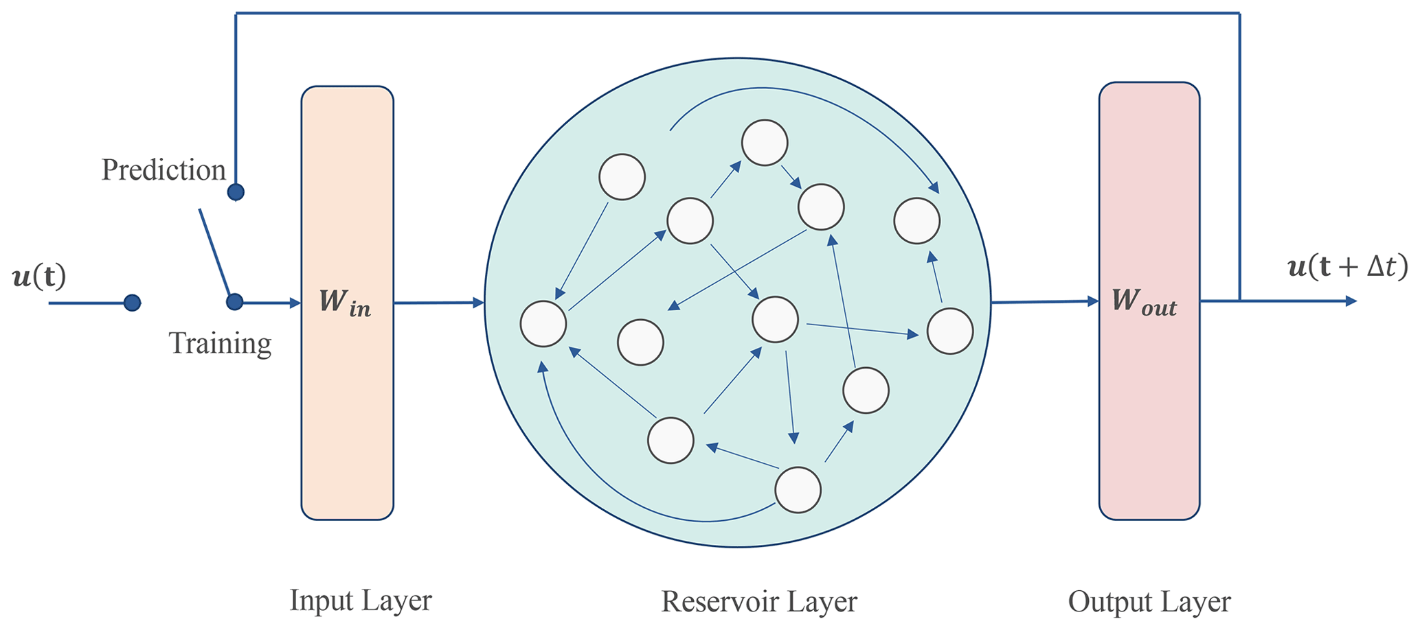
Figure 1The conceptual diagram of reservoir computing architecture. The network consists of an input layer, a hidden layer called reservoir, and an output layer.
For each grid point, observations to be assimilated are chosen. The rows or elements of yo, H, and R corresponding to non-assimilated observations should be removed as the localization procedure. “Smooth localization” can also be performed by multiplying some factors to each row of R based on the distance between target grid point and observation points (Hunt et al., 2007).
From the forecast ensemble, the mean and the covariance of the analysis ensemble can be calculated in the ensemble subspace as follows:
where stands for the mean and covariance of the analysis ensemble calculated in the ensemble subspace. They can be transformed into model space as follows:
On the other hand, as Eq. (6), we can consider the analysis covariance as the product of the analysis ensemble matrix:
where is the matrix whose ith column is the variation of the ith ensemble member from the mean for the analysis ensemble. Therefore, decomposing of Eq. (7) into the square root, we can get each analysis ensemble member at time k without explicitly computing the covariance matrix in the state space:
where is the ith column of in the first equation. A covariance inflation parameter is multiplied to take measures for the tendency of data assimilation to underestimate the uncertainty of state estimates by empirically accounting for model noise (see Eq. 3). See Hunt et al. (2007) for a more detailed derivation. Now, we can return to Eq. (5) and iterate forecast and analysis step.
As in the real application, we consider the situation that the observations are not available in the prediction period. Predictions are made by the model alone, using the latest analysis state variables as the initial condition:
where denotes the prediction variables at time k, is the prediction model (an imperfect L96 model), and is the mean of the analysis ensemble at the initial time of the prediction. This way of making prediction is called an “extended forecast”, and we call this prediction “LETKF-Ext” in this study, to distinguish it from the forecast–analysis iteration of LETKF.
2.3 Reservoir computing
2.3.1 Description of reservoir computing architecture
We use reservoir computing (RC) as the machine learning framework. RC is a type of recurrent neural network, which has a single hidden layer called reservoir. Figure 1 shows its architecture. As mentioned in Sect. 1, previous works have shown that RC can predict the dynamics of spatiotemporal chaotic systems.
The state of the reservoir layer at time step k is represented as a vector , which evolves given the input vector uk∈ℝm as follows:
where Win is the Dr×m input matrix which maps the input vector to the reservoir space, and A is the Dr×Dr adjacency matrix of the reservoir which determines the reservoir dynamics. Win should be determined to have only one nonzero component in each row, and each nonzero component is sampled from a uniform distribution of for some parameter a. A has a proportion of d nonzero components with random values from uniform distribution, and it is normalized to have the maximum eigenvalue ρ. The reservoir size Dr should be determined based on the size of the state space. From the reservoir state, we can compute the output vector v as follows:
where Wout is the m×Dr output matrix which maps the reservoir state to the state space, and is an operator of nonlinear transformation. The nonlinear transformation is essential for the accurate prediction (Chattopadhyay et al., 2020). It is important that A and Win are fixed and only Wout will be trained by just solving a linear problem. Therefore, the computational cost required to train RC is small and it is an outstanding advantage of RC compared to the other neural network frameworks.
In the training phase, we set the switch in Fig. 1 to the training configuration. Given a training data series , we can generate the reservoir state series using Eq. (12). By using the training data and reservoir state series, we can determine the Wout matrix by ridge regression. We minimize the following square error function with respect to Wout:
where ∥x∥=xTx and β is the ridge regression parameter (normally a small positive number). Since the objective function (Eq. 14) is quadratic, it is differentiable. The optimal value can be obtained by just solving a linear equation as follows:
where I is the Dr×Dr identity matrix and R,U are the matrices whose kth column is the vector f(rk),uk, respectively.
Then, we can shift to the predicting phase. Before we predict with the network, we first need to “spin up” the reservoir state. The spin-up process was done by giving the time series before the initial value to the network and calculating the reservoir state right before the beginning of the prediction via Eq. (12). After that, the output layer is connected to the input layer, and the network becomes recursive. In this configuration, the output value vk of Eq. (13) is used as the next input value uk of Eq. (12). Once we give the initial value u0, the network will iterate Eqs. (12) and (13) spontaneously, and the prediction will be yielded. At this point, RC can now be used as the surrogate model that mimics the state dynamics:
where denotes the prediction variables at time k, is the dynamics of RC (Eqs. 12 and 13) and is the time series of training data.
Considering the real application, it is natural to assume that the observation data can only be used as the training data and the initial value for the RC prediction. In this paper we call this type of prediction “RC-Obs”. Prediction time series here can be expressed using Eq. (16) as follows:
where is the observation time series and is the observation at the initial time of the prediction. As in Eq. (14), input and output of RC must be in the same space. Therefore, in this case, prediction variables have the same dimensionality as , and the non-observable grid points are not predicted by this prediction scheme.
2.3.2 Parallelized reservoir computing
In general, the required reservoir size Dr for accurate prediction increases as the dimension of the state space m increases. Since the RC framework needs to keep adjacency matrix A on the memory, and to perform inverse matrix calculation of Dr×Dr matrix (Eq. 15), an overly large reservoir size leads to unfeasible computational cost. Pathak et al. (2018b) proposed a solution to this issue, which is called the parallelized reservoir approach.
In this approach, the state space is divided into g groups, all of which contain state variables:
where is the ith group at time k, and uk,j is the jth state variable at time k. Each group is predicted by a different reservoir placed in parallel. The ith reservoir accepts the state variables of the ith group as well as adjacent l grids, which can be expressed as follows:
where is the input vector for the ith reservoir at time k. The dynamics of each reservoir can be expressed as follows according to Eq. (12):
where , A(i), , and are the reservoir state vector, adjacency matrix, input matrix, and output matrix for the ith reservoir. Each reservoir is trained independently using Eq. (13) so that
where is the output matrix in the ith reservoir. The prediction scheme of parallelized RC is summarized in Fig. 2. The strategy of parallelization is similar to the localization of data assimilation. As LETKF ignores correlations between distant grid points, parallelized reservoir computing assumes that the state variable of a grid point at the next time step depends only on the state variables of neighboring points. In contrast, ordinary RC assumes that the time evolution at one grid point is affected by all points in the state space, which may be inefficient in many applications in geoscience such as NWP.
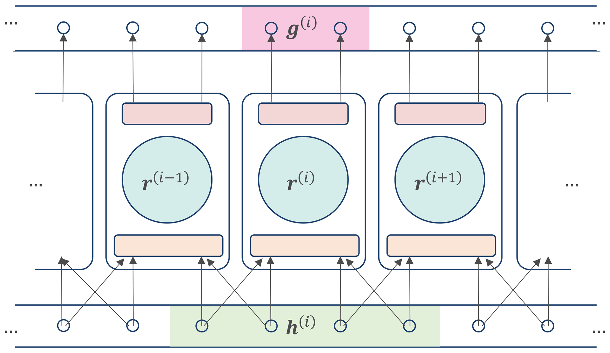
Figure 2The conceptual diagram of parallelized reservoir computing architecture. The state space is separated into some groups and the same number of reservoirs are shown parallel. Each reservoir group accepts the inputs from the corresponding group and some adjacent grids and predict the dynamics of the corresponding group.
2.4 Combination of RC and LETKF
As discussed so far and we will quantitatively discuss in the Sect. 4, LETKF-Ext and RC-Obs have contrasting advantages and disadvantages. LETKF-Ext can accurately predict even if the observation is noisy and/or sparsely distributed, while RC-Obs is vulnerable to the imperfectness in observation. On the other hand, LETKF-Ext can be strongly affected by the model biases since the prediction of LETKF-Ext depends only on the model after obtaining the initial condition, while RC-Obs has no dependence on the accuracy of the model as it only uses the observation data for training and prediction.
Therefore, the combination of LETKF and RC has the potential to push the limit of these two individual prediction methods and realize accurate and robust prediction. The weakness of RC-Obs is that we can only use the observational data directly, which is inevitably sparse in the real application, although RC is vulnerable to this imperfectness. In our proposed method, we make RC learn the analysis time series generated by LETKF instead of directly learning observation data.
Suppose we have sparse and noisy observations for the training data. If we take observations as inputs and analysis variables as outputs, LETKF can be considered as an operator to estimate the full state variables from the sparse observations:
where denotes the full-state variables (time series of the LETKF analysis ensemble mean), is the observation, and represents the state estimation operator, which is realized by LETKF in this study. Then, RC is trained by using as the training data set. In this way, RC can mimic the dynamics of analysis time series computed by the forecast–analysis cycle of LETKF. Prediction can be generated by using the analysis variables at the current time step () as the initial value. Since RC is trained with LETKF analysis variables, we call this method “RC-Anl”. By using the notation of Eq. (16), the prediction of RC-Anl can be expressed as follows:
where is the time series of the LETKF analysis variables. The schematics of the LETKF-Ext, RC-Obs, and RC-Anl are shown in Fig. 3. Initial values and model dynamics used in each method are compared in Table 1.
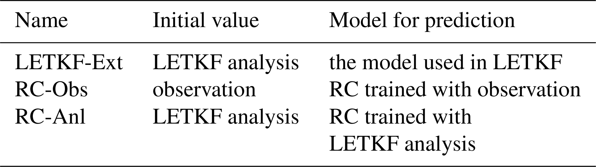

Figure 3The algorithm flow of LETKF-Ext, RC-Anl, and RC-Obs. Solid and dotted lines show the flow of variables and models (either process-based or data-driven surrogate), respectively.
Our proposed combination method is expected to predict more accurately than RC-Obs since the training data always exist in all the grid points, even if the observation is sparse. Also, especially if the model is substantially biased, the analysis time series generated by LETKF is more accurate than the model output itself. It means that RC-Anl is expected to be able to predict more accurately than LETKF-Ext.
To generate Nature Run, L96 with m=40 and F=8 was used, and it was numerically integrated by fourth-order Runge–Kutta method by time width Δt=0.005. Before calculating Nature Run, the L96 equation was integrated for 1 440 000 time steps for spin-up. In the following experiment, the F term in the model was changed to represent the model bias.
Here, we assume that the source of the model bias is unknown. When the source of bias is only the uncertainty in model parameters, and uncertain parameters which significantly induce the model bias are completely identified, optimization methods can estimate the value of the uncertain parameters to minimize the gaps between simulation and observation. This problem can also be solved by data assimilation methods (e.g., Bocquet and Sakov, 2013). However, it is difficult to calibrate the model when the source of uncertainty is unknown. Our proposed method does not need to identify the source of model bias so that it may be useful especially when the source of model bias is unknown. This is often the case in the large and complex models such as NWP systems.
The setting for LETKF was based on Miyoshi and Yamane (2007). As the localization process, the observation points within 10 indices are chosen to be assimilated for every grid point. The “smooth localization” is also performed on observation covariance R. Since we assume that each observation error is independent and thus R is diagonal, the localization procedure can be done just by dividing each diagonal element of observation covariance R by the value w calculated as follows:
where r is the distance between each observation point and each analyzed point. For every grid point, the observation points with w(r)≥0.0001 are chosen to be assimilated. In Eq. (10), a “covariance inflation factor”, which was set to 1.05 in our study, was multiplied to in each iteration to maintain the sufficiently large background error covariance by empirically accounting for model noise (see Eq. 3). Ensemble size Ne was set to 20.
The parameter values of parallelized RC used in this study are similar to Vlachas et al. (2020) but were slightly modified. Parameter settings used in the RC experiments are shown in Table 1. Jiang and Lai (2019) revealed that the performance of RC is sensitive to ρ and it needs to be tuned. We identified the proper value of ρ by sensitivity studies. Other parameters do not substantially affect the prediction accuracy, and we selected them based on the settings in previous works such as Vlachas et al. (2020). The nonlinear transformation function for the output layer in Eq. (13) is the same as Chattopadhyay et al. (2020), which is represented as follows:
where ri is the ith element of r. Note that the form of the transformation function can be flexible; one can use a different form of the function to predict Lorenz 96 (Chattopadhyay et al., 2020), or the same function can be used to predict other systems (Pathak et al., 2017). In the prediction phase, we used the data for 100 time steps before the prediction initial time for the reservoir spin-up.
We implement numerical experiments to investigate the performance of RC-Obs, LETKF-Ext, and RC-Anl to predict L96 dynamics. First, we evaluate the performance of RC-Obs under perfect observations (all the grid points are observed with no error) and quantify the effect of the observation imperfectness (i.e., observation error and spatiotemporal sparsity), to investigate the prediction skill of the standalone use of RC and LETKF. Second, we evaluate the performance of RC-Anl. We investigate the performance of RC-Anl and LETKF-Ext as the functions of the observation density and model biases.
In each experiment, we prepare 200 000 time steps of Nature Run. The first 100 000 time steps are used for the training of RC or for the spinning up of LETKF, and the rest of them are used for the evaluation of each method. Every prediction is repeated 100 times to avoid the effect of the heterogeneity of data. For the LETKF-Ext prediction, the analysis time series of all the evaluation data is first generated. Then, the analysis variables for one every 1000 time step are taken as the initial conditions and in total 100 prediction runs are performed. For the RC-Obs prediction, evaluation data are equally divided into 100 sets and the prediction is identically done for each set. For the RC-Anl prediction, the analysis time series of training data are used for training, and the prediction is performed using the same initial condition as LETKF-Ext. Each prediction set of LETKF-Ext, RC-Obs, and RC-Anl corresponds to the same time range.
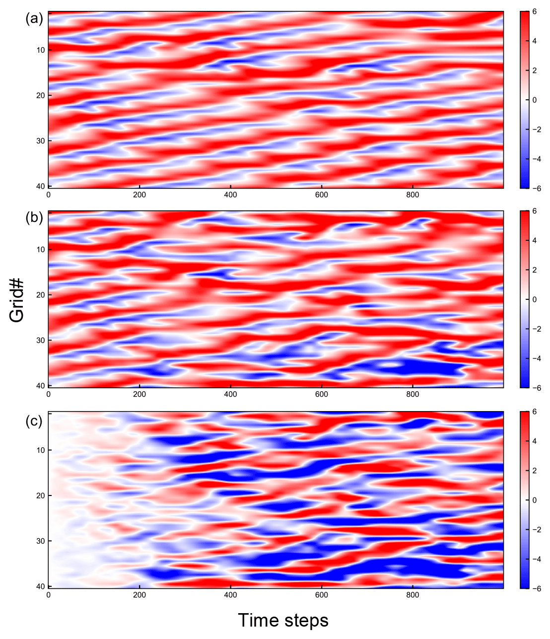
Figure 4The Hovmöller diagram of (a) Nature Run, (b) a prediction of RC-Obs, and (c) difference between (a) and (b). Horizontal axis shows the time steps and vertical axis shows the nodal number. Value at each time step and node is represented by the color.
The prediction accuracy of each method is evaluated by taking the average of RMSE of 100 sets for each time step. We call this metric mean RMSE (mRMSE), and it can be represented as follows:
where t is the number of the steps elapsed from the prediction initial time, is the jth nodal value of the ith prediction set at time t, and is the corresponding value of Nature Run. Using this metric, we can see how the prediction accuracy is degraded as time elapses from initial time (so-called “forecast lead time”).
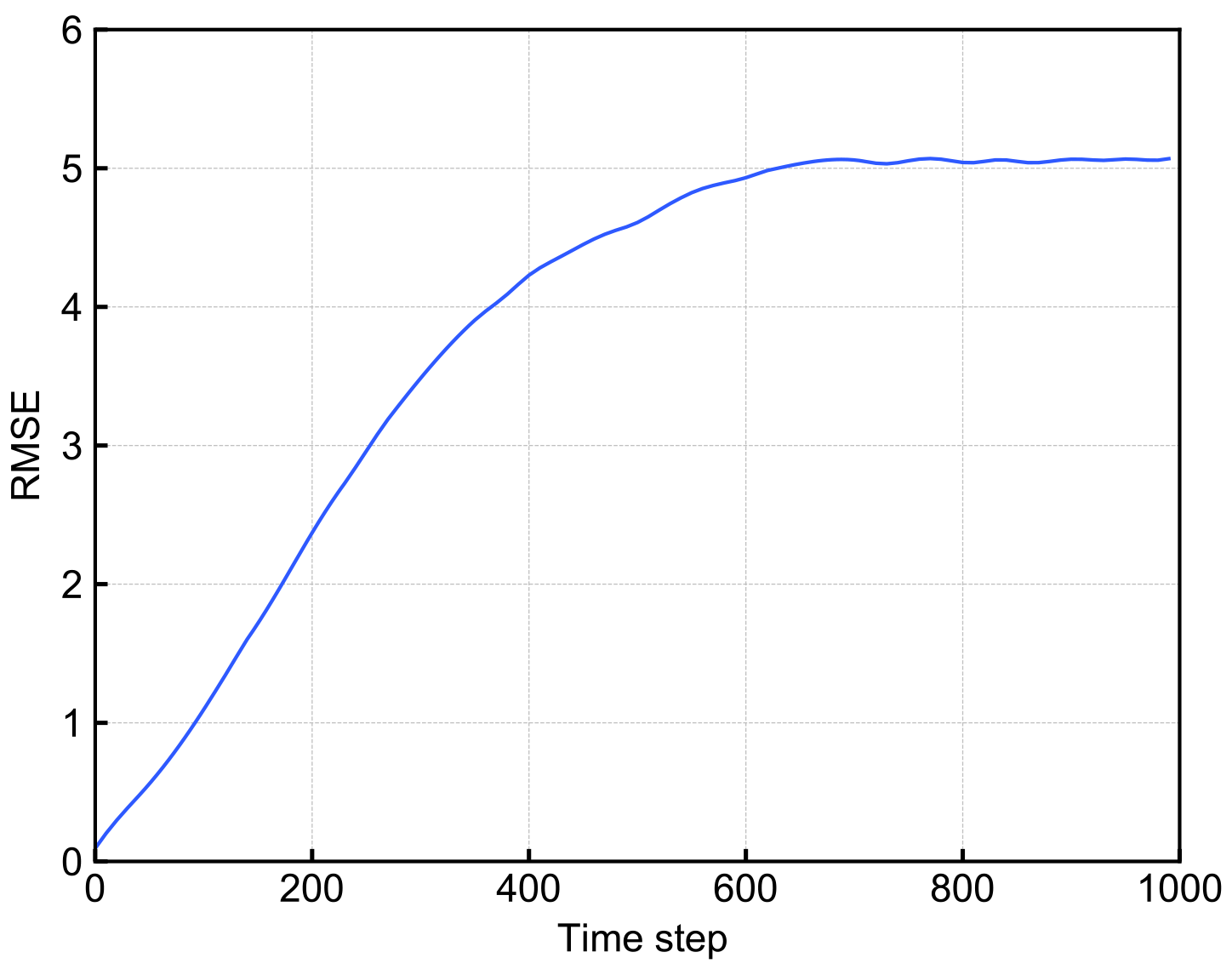
Figure 5The mRMSE time series of the predictions of RC-Obs with perfect observation. Horizontal axis shows the time step and vertical axis shows the value of mRMSE.
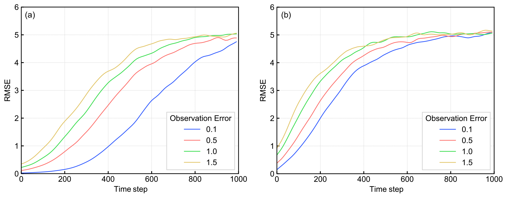
Figure 6The mRMSE time series of the predictions of (a) LETKF-Ext and (b) RC-Obs with noisy observation. Each color corresponds to the observation error indicated by the legend.

Figure 7The mRMSE time series of the predictions of (a) LETKF-Ext and (b) RC-Obs with spatially sparse observation. Each color corresponds to the number of the observation points.
Figure 4 shows the Hovmöller diagram of a prediction of RC-Obs and Nature Run. Figure 4 also shows the difference between prediction and Nature Run, as well as the actual prediction results so that we can see how long we can keep the prediction accurate. RC is trained with perfect observation (e=0 at all grid points). Figure 4 shows that RC-Obs predicts accurately within approximately 200 time steps.
Figure 5 shows the time variation of the mRMSE (see Eq. 26) of RC-Obs with perfect observation. It also shows that RC-Obs can predict with good accuracy for approximately 200 time steps. It should be noted that LETKF (as well as other data assimilation methods) just replaces the model's forecast with the initial conditions identical to Nature Run when all state variables can be perfectly observed, and thus the prediction accuracy of LETKF-Ext will be perfect if we have no model bias. LETKF-Ext is much superior to RC-Obs under this regime (not shown).
Next, we evaluated the sensitivity of the prediction skill of both LETKF-Ext and RC-Obs to the imperfectness of the observations. Figure 6a and b show the effect of the observation error on the prediction skill. The value of observation error e is changed from 0.1 to 1.5 and the mRMSE time series is drawn. We can see that LETKF-Ext is more sensitive to the increase in observation error than RC-Obs, although LETKF-Ext is superior in accuracy to RC-Obs within this range of observation error.
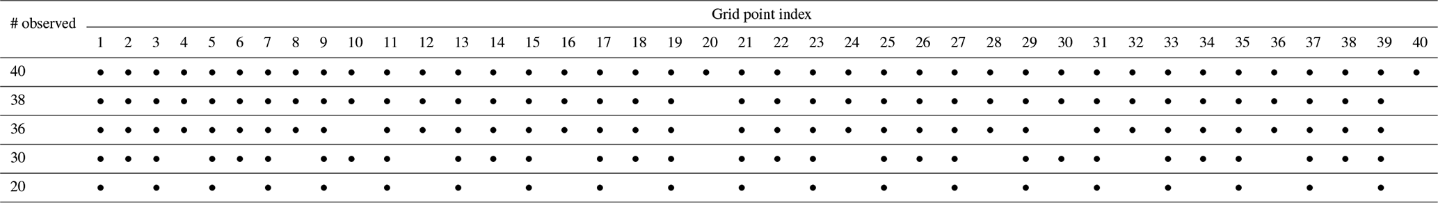
However, RC-Obs showed a greater sensitivity to the density of observation points than LETKF-Ext. Figure 7a and b show the sensitivity of the prediction accuracy of LETKF-Ext and RC-Obs, respectively, to the number of observed grid points. Observation is reduced as uniformly as possible. The observation network in each experiment is shown in Table 3. Even though we can observe a small part of the system, the accuracy of LETKF-Ext changed only slightly. On the other hand, the accuracy of RC-Obs gets worse when we remove a few observations. As assumed in the Sect. 2.4, we verified that RC-Obs is more sensitive to the observation sparsity than LETKF-Ext.
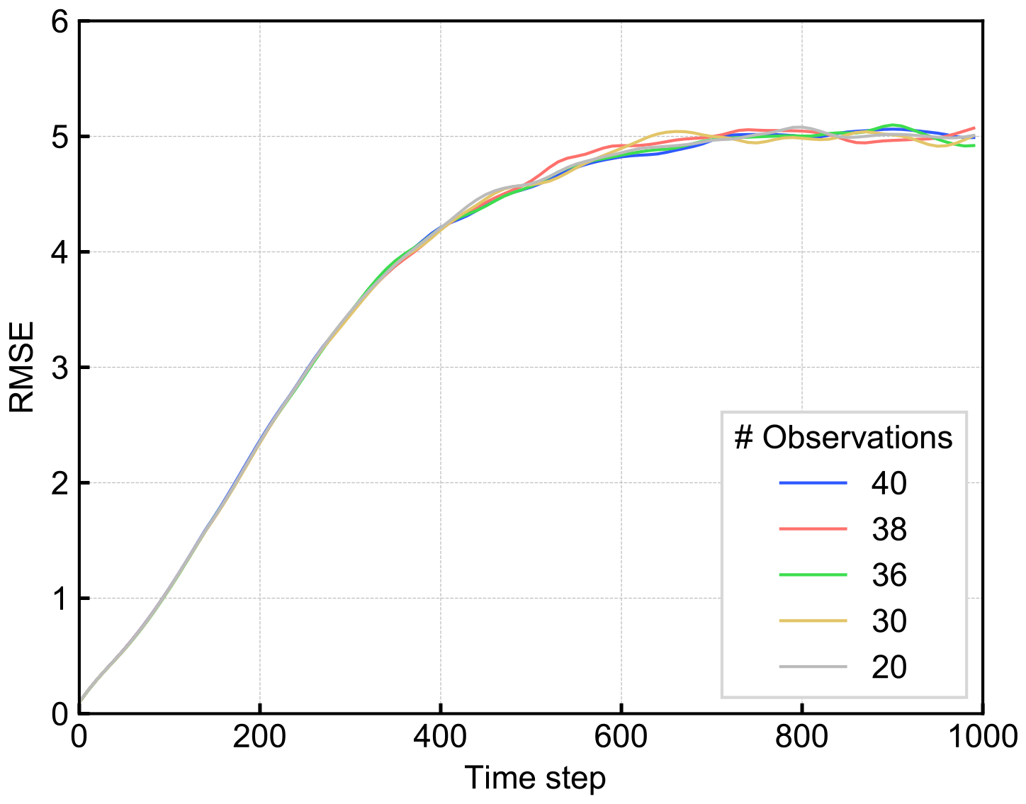

We tested the prediction skill of our newly proposed method, RC-Anl, under perfect models and sparse observations. Here, we used the observation error e=1.0. Figure 8 shows the change of the mRMSE time series of RC-Anl with the different number of observed grid points. It indicates that the vulnerability of the prediction accuracy to the change of the number of observed grid points, which is found in RC-Obs, no longer exists in RC-Anl. Although the prediction accuracy is lower than LETKF-Ext (Fig. 7a), our new method indicates a robustness to the observation sparsity and overcomes the limitation of the standalone RC.
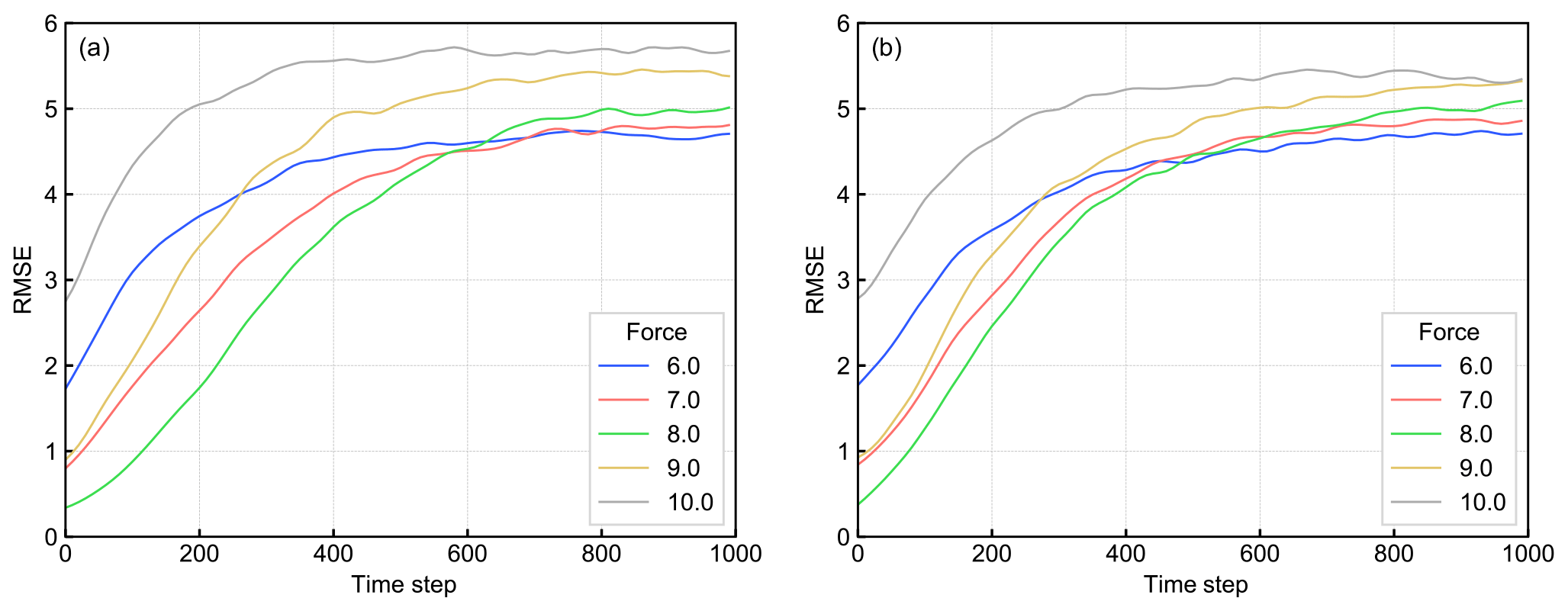
Figure 9The mRMSE time series of the predictions of (a) LETKF-Ext and (b) RC-Anl with a biased model. Each color corresponds to each value of the F term.
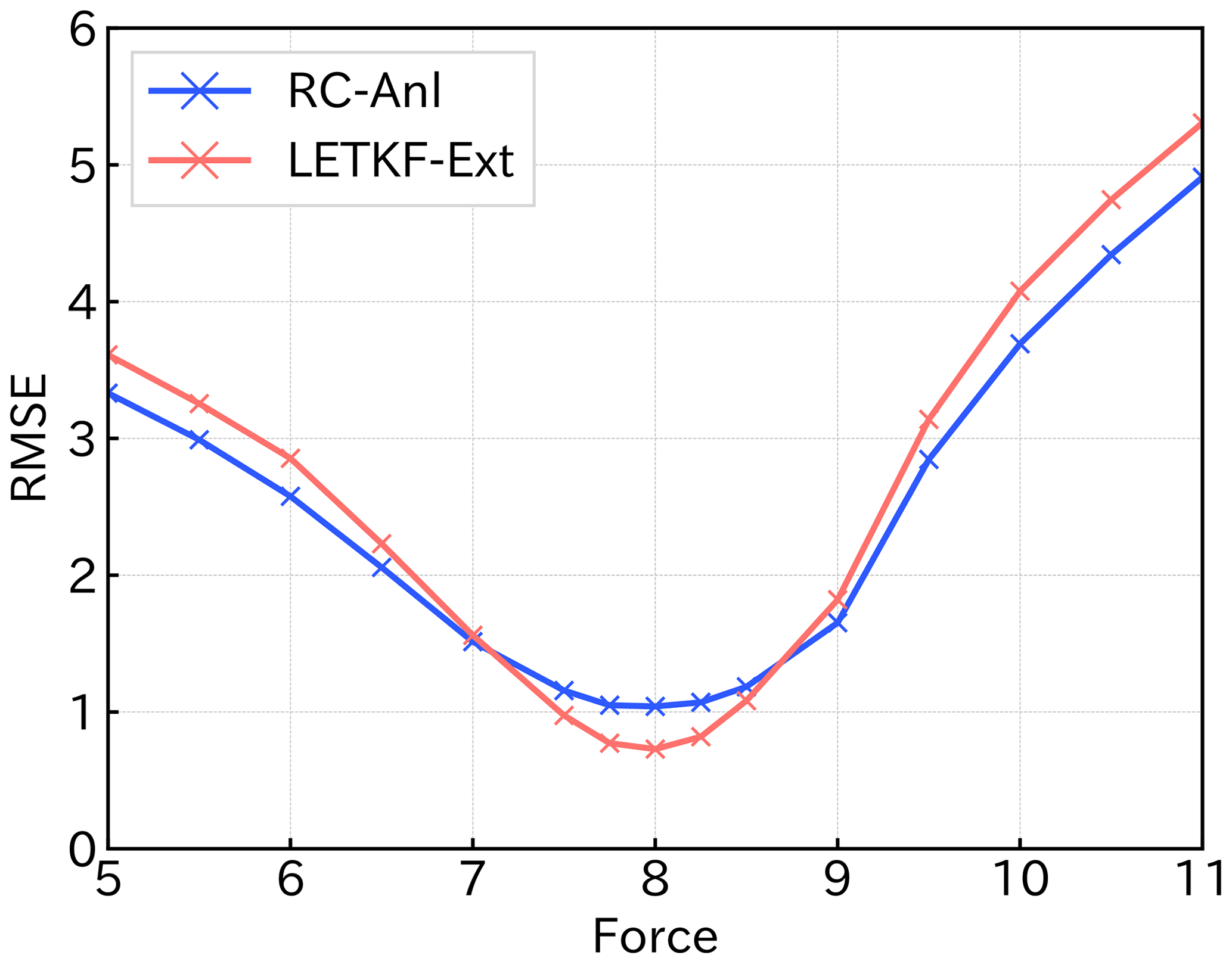
Figure 10The mRMSE(80) of the predictions of LETKF-Ext(red) and RC-Anl(blue) for each model bias. Horizontal axis shows the value of the force parameter of Eq. (1) (8 is the true value) and vertical axis shows the value of mRMSE.
Moreover, when the model used in LETKF is biased, RC-Anl outperforms LETKF-Ext. Figure 9a and b show the change of the mRMSE time series when changing the model biases. The number of the observed points was set to 20. The F term in Eq. (1) was changed from the true value 8 (the F value of the model for Nature Run) to values in [5.0,11.0] as the model bias, and the accuracy of LETKF-Ext and RC-Anl is plotted. The accuracy of LETKF-Ext was slightly better than that of RC-Anl when the model was not biased (F=8; green line). However, when the bias is large (e.g., F=10; gray line), RC-Anl showed the better prediction accuracy.
We confirmed this result by comparing the mRMSE value of RC-Anl and LETKF-Ext at the specific forecast lead time. Figure 10 shows the value of mRMSE(80) (see Eq. 26) as the function of the value of the F term. Both lines that show the skill of RC-Anl (blue) and LETKF-Ext (red) are convex downward and have a minimum at F=8, meaning that the accuracy of both prediction methods is the best when the model is not biased. In addition, as long as the F value is in the interval [7.5,8.5], LETKF-Ext has better accuracy than RC-Anl. However, if the model bias becomes larger than that, RC-Anl becomes more accurate than LETKF-Ext. As the bias increases, the difference between the mRMSE(80) of two methods becomes larger, and the superiority of RC-Anl becomes more obvious. We found that RC-Anl can predict more accurately than LETKF-Ext when the model is biased.
We also checked the robustness for the training data size. Figure 11 shows the change of the accuracy of RC-Anl by changing the size of training data from 100 000 to 10 000 time steps. We confirmed that the prediction accuracy did not change until the size was reduced to 25 000 time steps. Although we have used a large amount of training data (100 000 time steps; 68 model years) so far, the results are robust to the reduction of the size of the training data.
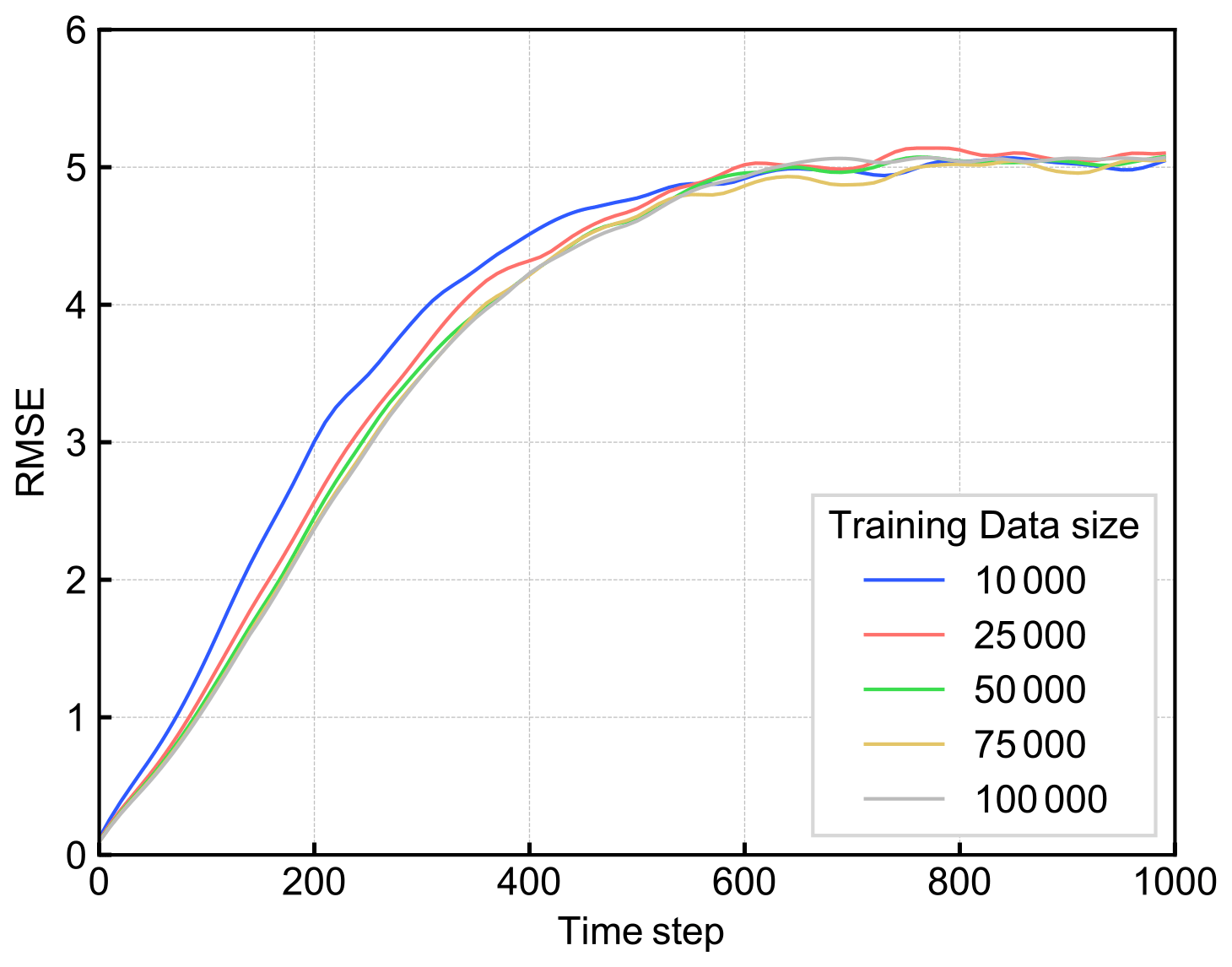
Figure 11The mRMSE time series of the predictions of RC-Anl with various lengths of training data, with perfect observations and a perfect model. Each color corresponds to the value of the size of training data.
By comparing the prediction skill of RC-Obs and LETKF-Ext, we confirmed that RC-Obs can predict with accuracy comparable to LETKF-Ext, if we have perfect observations. This result is consistent with Chattopadhyay et al. (2020), Pathak et al. (2017), and Vlachas et al. (2020), and we can expect that RC has the potential to predict various kinds of spatiotemporal chaotic systems.
However, Vlachas et al. (2020) revealed that the prediction accuracy of RC is substantially degraded when the observed grid points are reduced, compared to other machine learning techniques such as LSTM. Our result is consistent with their study. In contrast, Chattopadhyay et al. (2020) showed that RC can predict the multi-scale chaotic system correctly even though only the largest-scale dynamics is observed. Comparing these results, we can suggest that the states in the scale of dominant dynamics should be observed almost perfectly to accurately predict the future state by RC. Therefore, when we use RC to predict spatiotemporal chaotic systems with sparse observation data, we need to interpolate them to generate the appropriate training data. However, the interpolated data inevitably include errors even if the observation data itself have no error, so it should be verified that RC can predict accurately by training data with some errors. Previous works such as Chattopadhyay et al. (2020), Pathak et al. (2017), or Vlachas et al. (2020) have not considered the impact of error in the training data. We found that the prediction accuracy of RC degrades as the error in training data grows, but the degradation rate is not so large (if all the training data of all the grid points are obtained). We can expect from this result that RC trained with the interpolated observation data can predict accurately to some extent, but the interpolated data should be as accurate as possible.
In this study, LETKF was used to prepare the training data for RC, since LETKF can interpolate the observations and reduce their error at the same time. We showed that our proposed approach works correctly. Brajard et al. (2020) also made a CNN learn the dynamics from sparse observation data and successfully predict the dynamics of the L96 model. However, as mentioned in the introduction section, Brajard et al. (2020) iterated the learning and data assimilation until they converge, because it replaced the model used in data assimilation with CNN. Although their model-free method has an advantage that it was not affected by the process-based model's reproducibility of the phenomena, it can be computationally expensive since the number of iterations can be relatively large. By contrast, we need to train RC just one time, because we use the process-based model (i.e., data assimilation method) to prepare the training data. We overcome the problem of computational feasibility.
Note also that the computational cost of training RC is much lower than the other neural networks. Since the framework of our method does not depend on a specific machine learning framework, we believe that we can flexibly choose other machine learning methods such as RNN, LSTM, ANN, etc. Previous studies such as Chattopadhyay et al. (2020) or Vlachas et al. (2020) revealed that these methods show competitive performances compared to RC in predicting spatiotemporal chaos. Using them instead of RC in our method would probably give similar results. However, the advantage of RC is its cheap training procedure. RC does not need to perform an expensive back-propagation method for training, unlike other neural networks (Chattopadhyay et al., 2020; Lu et al., 2017). Therefore, RC is considered as a promising tool for predicting spatiotemporal chaos. Although our method has flexibility in the choice of machine learning methods, we consider that the good performance with RC is important in this research context.
The good performance of our proposed method supports the suggestion of Dueben and Bauer (2018), in which machine learning should be applied to the analysis data generated by data assimilation methods as the first step of the application of machine learning to weather prediction. As Weyn et al. (2019) did, we successfully trained the machine learning model with the analysis data.
Most importantly, we also found that the prediction by RC-Anl is more robust to the model biases than the extended forecast by LETKF (i.e., LETKF-Ext). This result suggests that our method can be beneficial in various real problems, as the model in real applications inevitably contains some biases. Pathak et al. (2018a) developed the hybrid prediction system of RC and a biased model. Although Pathak et al. (2018a) successfully predicted the spatiotemporal chaotic systems using the biased models, they needed perfect observations to train their RC. The advantage of our proposed method compared to these RC studies is that we allow both models and observation networks to be imperfect. As in the review by Karniadakis et al. (2021), methodologies to train the dynamics from noisy observational data by integrating data and physical knowledge are attracting attention. In the NWP context, some studies proposed methods to combine data assimilation and machine learning to emulate the system dynamics from imperfect models and observations (e.g., Bocquet et al., 2019, 2020; Brajard et al., 2020; Dueben and Bauer, 2018), and these approaches are getting popular. Our study significantly contributes to this emerging research field.
Although we tested our method only on the 40-dimensional Lorenz 96 system, Pathak et al. (2018b) indicated that parallelized RC can be extended to predict the dynamics of substantially high dimensional chaos such as a 200-dimensional Kuramoto–Sivashinski equation with small computational costs. Moreover, the applicability to the realistic NWP problems has also been discussed in their sequel study (Wikner et al., 2020). These studies imply that the findings of this study can also be applied to higher-dimensional systems.
In NWP problems, it is often the case that homogenous observation data of high resolution are not available over a wide range of time and space, which can be an obstacle to applying machine learning to NWP tasks (Dueben and Bauer, 2018). We revealed that RC is robust for the temporal sparsity of observations, and RC can be trained with relatively small training data sets.
However, since the Lorenz 96 model (and other conceptual models such as the Kuramoto–Sivashinski equation) is ergodic, it is unclear whether our method can be applied to real NWP problems directly, which are possibly non-ergodic. Although our proposed method has the potential to extend to larger and more complex problems, further studies are needed.
The prediction skills of the extended forecast with LETKF (LETKF-Ext), RC that learned the observation data (RC-Obs), and RC that learned the LETKF analysis data (RC-Anl) were evaluated under imperfect models and observations, using the Lorenz 96 model. We found that the prediction by RC-Obs is substantially vulnerable to the sparsity of the observation network. Our proposed method, RC-Anl, can overcome this vulnerability. In addition, RC-Anl could predict more accurately than LETKF-Ext when the process-based model is biased. Our new method is robust to the imperfectness of both models and observations and we might obtain similar results in higher-dimensional and more complex systems. Further studies on more complicated models or operational atmospheric models are expected.
The source code for RC and Lorenz96 model is available at https://doi.org/10.5281/zenodo.3907291 and for LETKF at https://github.com/takemasa-miyoshi/letkf (Miyoshi, 2016).
All the data used in this study can be calculated using the model source code.
The conception and design of this work and the data interpretation were done by FT and YS. FT was responsible for the development of the model source codes, the execution of all model runs, and the paper preparation. YS provided critical comments on the paper.
The authors declare that they have no conflict of interest.
Publisher’s note: Copernicus Publications remains neutral with regard to jurisdictional claims in published maps and institutional affiliations.
This research has been supported by the Japan Society for the Promotion of Science (grant nos. JP17K18352 and JP18H03800), the JAXA (grant no. ER2GWF102), the JST AIP (grant no. JPMJCR19U2), and the JST FOREST program (grant no. JPMJFR205Q).
This paper was edited by Adrian Sandu and reviewed by four anonymous referees.
Asanjan, A., Yang, T., Hsu, K., Sorooshian, S., Lin, J., and Peng, Q.: Short-Term Precipitation Forecast Based on the PERSIANN System and LSTM Recurrent Neural Networks, J. Geophys. Res.-Atmos., 123, 12543–12563, https://doi.org/10.1029/2018JD028375, 2018.
Bannister, R. N.: A review of operational methods of variational and ensemble-variational data assimilation, Q. J. Roy. Meteor. Soc., 143, 607–633, https://doi.org/10.1002/qj.2982, 2017.
Bocquet, M. and Sakov, P.: Joint state and parameter estimation with an iterative ensemble Kalman smoother, Nonlin. Processes Geophys., 20, 803–818, https://doi.org/10.5194/npg-20-803-2013, 2013.
Bocquet, M., Brajard, J., Carrassi, A., and Bertino, L.: Data assimilation as a learning tool to infer ordinary differential equation representations of dynamical models, Nonlin. Processes Geophys., 26, 143–162, https://doi.org/10.5194/npg-26-143-2019, 2019.
Bocquet, M., Farchi, A., and Malartic, Q.: Online learning of both state and dynamics using ensemble Kalman filters, Found. Data Sci., https://doi.org/10.3934/fods.2020015, 2020.
Brajard, J., Carrassi, A., Bocquet, M., and Bertino, L.: Combining data assimilation and machine learning to emulate a dynamical model from sparse and noisy observations: a case study with the Lorenz 96 model, J. Comput. Sci., 44, 101171, https://doi.org/10.1016/j.jocs.2020.101171, 2020.
Chattopadhyay, A., Hassanzadeh, P., and Subramanian, D.: Data-driven predictions of a multiscale Lorenz 96 chaotic system using machine-learning methods: reservoir computing, artificial neural network, and long short-term memory network, Nonlin. Processes Geophys., 27, 373–389, https://doi.org/10.5194/npg-27-373-2020, 2020.
Dueben, P. D. and Bauer, P.: Challenges and design choices for global weather and climate models based on machine learning, Geosci. Model Dev., 11, 3999–4009, https://doi.org/10.5194/gmd-11-3999-2018, 2018.
Hochreiter, S. and Schmidhuber, J.: Long Short-Term Memory, Neural Comput., 9, 1735–1780, https://doi.org/10.1162/neco.1997.9.8.1735, 1997.
Houtekamer, P. L. and Zhang, F.: Review of the ensemble Kalman filter for atmospheric data assimilation, Mon. Weather Rev., 144, 4489–4532, https://doi.org/10.1175/MWR-D-15-0440.1, 2016.
Hunt, B. R., Kostelich, E. J., and Szunyogh, I.: Efficient data assimilation for spatiotemporal chaos: A local ensemble transform Kalman filter, Phys. D Nonlinear Phenom., 230, 112–126, https://doi.org/10.1016/j.physd.2006.11.008, 2007.
Jaeger, H. and Haas, H.: Harnessing Nonlinearity: Predicting Chaotic Systems and Saving Energy in Wireless Communication, Science, 304, 78–80, 2004.
Jiang, J. and Lai, Y.-C.: Model-free prediction of spatiotemporal dynamical systems with recurrent neural networks: Role of network spectral radius, Phys. Rev. Res., 1, 33056, https://doi.org/10.1103/physrevresearch.1.033056, 2019.
Karniadakis, G. E., Kevrekidis, I. G., Lu, L., Perdikaris, P., Wang, S., and Yang, L.: Physics-?informed machine learning, Nat. Rev. Phys., 3, 422–440, https://doi.org/10.1038/s42254-021-00314-5, 2021.
Kotsuki, S., Greybush, S. J., and Miyoshi, T.: Can we optimize the assimilation order in the serial ensemble Kalman filter? A study with the Lorenz-96 model, Mon. Weather Rev., 145, 4977–4995, https://doi.org/10.1175/MWR-D-17-0094.1, 2017.
Lorenz, E. N. and Emanuel, K. A.: Optimal sites for supplementary weather observations: Simulation with a small model, J. Atmos. Sci., 55, 399–414, https://doi.org/10.1175/1520-0469(1998)055<0399:OSFSWO>2.0.CO;2, 1998.
Lu, Z., Pathak, J., Hunt, B., Girvan, M., Brockett, R., and Ott, E.: Reservoir observers: Model-free inference of unmeasured variables in chaotic systems, Chaos, 27, 041102, https://doi.org/10.1063/1.4979665, 2017.
Miyoshi, T.: Ensemble kalman filter experiments with a primitive-equation global model, PhD Diss. Univ. Maryland, Coll. Park, 197 pp., 2005.
Miyoshi, T.: Source code for Local Ensemble Transform Kalman Filter, github [code], available at: https://github.com/takemasa-miyoshi/letkf, last access: 2016.
Miyoshi, T. and Yamane, S.: Local ensemble transform Kalman filtering with an AGCM at a T159/L48 resolution, Mon. Weather Rev., 135, 3841–3861, https://doi.org/10.1175/2007MWR1873.1, 2007.
Nguyen, D. H. and Bae, D. H.: Correcting mean areal precipitation forecasts to improve urban flooding predictions by using long short-term memory network, J. Hydrol., 584, 124710, https://doi.org/10.1016/j.jhydrol.2020.124710, 2020.
Pathak, J., Lu, Z., Hunt, B. R., Girvan, M., and Ott, E.: Using machine learning to replicate chaotic attractors and calculate Lyapunov exponents from data, Chaos, 27, 121102, https://doi.org/10.1063/1.5010300, 2017.
Pathak, J., Wikner, A., Fussell, R., Chandra, S., Hunt, B. R., Girvan, M. and Ott, E.: Hybrid forecasting of chaotic processes: Using machine learning in conjunction with a knowledge-based model, Chaos, 28, 041101, https://doi.org/10.1063/1.5028373, 2018a.
Pathak, J., Hunt, B., Girvan, M., Lu, Z., and Ott, E.: Model-Free Prediction of Large Spatiotemporally Chaotic Systems from Data: A Reservoir Computing Approach, Phys. Rev. Lett., 120, 024102, https://doi.org/10.1103/PhysRevLett.120.024102, 2018b.
Penny, S. G.: The hybrid local ensemble transform Kalman filter, Mon. Weather Rev., 142, 2139–2149, https://doi.org/10.1175/MWR-D-13-00131.1, 2014.
Raboudi, N. F., Ait-El-Fquih, B., and Hoteit, I.: Ensemble Kalman filtering with one-step-ahead smoothing, Mon. Weather Rev., 146, 561–581, https://doi.org/10.1175/MWR-D-17-0175.1, 2018.
Rajendra, P. and Brahmajirao, V.: Modeling of dynamical systems through deep learning, Biophys. Rev., 12, 1311–1320, https://doi.org/10.1007/s12551-020-00776-4, 2020.
Sawada, Y., Okamoto, K., Kunii, M., and Miyoshi, T.: Assimilating Every-10-minute Himawari-8 Infrared Radiances to Improve Convective Predictability, J. Geophys. Res.-Atmos., 124, 2546–2561, https://doi.org/10.1029/2018JD029643, 2019.
Schraff, C., Reich, H., Rhodin, A., Schomburg, A., Stephan, K., Periáñez, A., and Potthast, R.: Kilometre-scale ensemble data assimilation for the COSMO model (KENDA), Q. J. Roy. Meteor. Soc., 142, 1453–1472, https://doi.org/10.1002/qj.2748, 2016.
Tomizawa, F.: f-tomizawa/RC_Analysis_Loren96 v1.0 (v1.0), Zenodo, https://doi.org/10.5281/zenodo.3907291, 2020.
Vlachas, P. R., Byeon, W., Wan, Z. Y., Sapsis, T. P., and Koumoutsakos, P.: Data-driven forecasting of high-dimensional chaotic systems with long short-Term memory networks, Proc. R. Soc. A Math. Phys. Eng. Sci., 474, 20170844, https://doi.org/10.1098/rspa.2017.0844, 2018.
Vlachas, P. R., Pathak, J., Hunt, B. R., Sapsis, T. P., Girvan, M., Ott, E., and Koumoutsakos, P.: Backpropagation algorithms and Reservoir Computing in Recurrent Neural Networks for the forecasting of complex spatiotemporal dynamics, Neural Networks, 126, 191–217, https://doi.org/10.1016/j.neunet.2020.02.016, 2020.
Weyn, J. A., Durran, D. R., and Caruana, R.: Can Machines Learn to Predict Weather? Using Deep Learning to Predict Gridded 500-hPa Geopotential Height From Historical Weather Data, J. Adv. Model. Earth Syst., 11, 2680–2693, https://doi.org/10.1029/2019MS001705, 2019.
Wikner, A., Pathak, J., Hunt, B., Girvan, M., Arcomano, T., Szunyogh, I., Pomerance, A., and Ott, E.: Combining machine learning with knowledge-based modeling for scalable forecasting and subgrid-scale closure of large, complex, spatiotemporal systems, Chaos, 30, 053111, https://doi.org/10.1063/5.0005541, 2020.
Yokota, S., Seko, H., Kunii, M., Yamauchi, H., and Sato, E.: Improving Short-Term Rainfall Forecasts by Assimilating Weather Radar Reflectivity Using Additive Ensemble Perturbations, J. Geophys. Res.-Atmos., 123, 9047–9062, https://doi.org/10.1029/2018JD028723, 2018.
Zhang, F., Minamide, M., and Clothiaux, E. E.: Potential impacts of assimilating all-sky infrared satellite radiances from GOES-R on convection-permitting analysis and prediction of tropical cyclones, Geophys. Res. Lett., 43, 2954–2963, https://doi.org/10.1002/2016GL068468, 2016.