the Creative Commons Attribution 4.0 License.
the Creative Commons Attribution 4.0 License.
 | 09 Sep 2021
Australian tidal currents – assessment of a barotropic model (COMPAS v1.3.0 rev6631) with an unstructured grid
Mike Herzfeld
Mark Hemer
Darren Engwirda
While the variations of tidal range are large and fairly well known across Australia (less than 1 m near Perth but more than 14 m in King Sound), the properties of the tidal currents are not. We describe a new regional model of Australian tides and assess it against a validation dataset comprising tidal height and velocity constituents at 615 tide gauge sites and 95 current meter sites. The model is a barotropic implementation of COMPAS, an unstructured-grid primitive-equation model that is forced at the open boundaries by TPXO9v1. The mean absolute error (MAE) of the modelled M2 height amplitude is 8.8 cm, or 12 % of the 73 cm mean observed amplitude. The MAE of phase (10∘), however, is significant, so the M2 mean magnitude of vector error (MMVE, 18.2 cm) is significantly greater. The root sum square over the eight major constituents is 26 % of the observed amplitude. We conclude that while the model has skill at height in all regions, there is definitely room for improvement (especially at some specific locations). For the M2 major axis velocity amplitude, the MAE across the 95 current meter sites, where the observed amplitude ranges from 0.1 to 156 cm s−1, is 6.9 cm s−1, or 22 % of the 31.7 cm s−1 observed mean. This nationwide average result is encouraging, but it conceals a very large regional variation. Relative errors of the tidal current amplitudes on the narrow shelves of New South Wales (NSW) and Western Australia exceed 100 %, but tidal currents are weak and negligible there compared to non-tidal currents, so the tidal errors are of little practical significance. Looking nationwide, we show that the model has predictive value for much of the 79 % of Australia's shelf seas where tides are a major component of the total velocity variability. In descending order this includes the Bass Strait, the Kimberley to Arnhem Land, and southern Great Barrier Reef regions. There is limited observational evidence to confirm that the model is also valuable for currents in other regions across northern Australia. We plan to commence publishing “unofficial” tidal current predictions for chosen regions in the near future based on both our COMPAS model and the validation dataset we have assembled.
- Article
(32969 KB) - Full-text XML
- BibTeX
- EndNote


Tidal currents are a major component of the velocity variability for most of the Australian continental shelf, yet tidal current predictions are only listed in the Australian National Tide Tables for seven sites, five of which are in Torres Strait. As part of a project to map Australia's tidal energy resource and as a step towards an operational, model-based tidal current forecasting ability, we have compiled a tidal current harmonic constituent validation dataset at 95 sites based on observations acquired by a number of agencies. This is a significant number of sites, but it is still small compared to the 683 sites for which the Bureau of Meteorology Tidal Unit has estimates of tidal height harmonic constituents. We use these validation datasets for currents and heights to assess the errors of a newly configured barotropic implementation of an unstructured-grid tidal model for the Australian continental shelf. This tells us how well the tidal component of the total variability can be predicted. Taking non-tidal currents into account as well, we identify the regions of Australia where model-based tidal current predictions are not only accurate, but also a large part of the total variability.
As mentioned above, the work reported here was done for two reasons: (1) to identify regions where tidal currents are prospective from a renewable energy point of view and (2) to lay the foundations of a more general-purpose national model of the tidal currents of Australia. The model we used is called COMPAS (Coastal Ocean Marine Prediction Across Scales). It is a fully non-linear 3D model that has been described in full by Herzfeld et al. (2020a). In this paper, we assess the ability of this model to simulate barotropic tides (both currents and sea level) as a first step towards a baroclinic model of the tides and then a baroclinic model with non-tidal flows as well.
COMPAS was chosen over structured model counterparts due to its capacity for superior resolution placement and transition, allowing high resolution to be placed in areas of interest and low resolution elsewhere. This significantly reduces the number of cells required to model such a large domain, resulting in an acceptable computational cost. COMPAS is a coastal ocean model designed to be used at scales ranging from estuaries to regional ocean domains. It is a three-dimensional (3D) finite-volume hydrodynamic model based on the 3D equations of momentum, continuity, and conservation of heat and salt, employing the hydrostatic and Boussinesq approximations. The equations of motion are discretised on arbitrary polygonal meshes according to the TRiSK numerics (Thuburn et al., 2009; Ringler et al., 2010), which is a generalisation of the standard Arakawa C-grid scheme to unstructured meshes. The horizontal terms in the governing equations (momentum advection, horizontal mixing, and Coriolis) are discretised using the TRiSK numerics, whereas the pressure gradient and vertical mixing are discretised using the finite-difference approach outlined by Herzfeld (2006). While COMPAS uses the same TRiSK C-grid discretisation as MPAS, it is a different model and code optimised for coastal applications, and in these regions it does not share certain limitations specific to MPAS-O. However, like MPAS, the horizontal mesh must be an orthogonal, centroidal, and well-centred “primal-dual” tessellation, typically consisting of collections of Voronoi cells and their dual Delaunay triangles. The 3D model may operate using z or s vertical coordinates; however, in the present application a depth-averaged configuration is used, as mentioned above. The bottom topography is represented using partial cells. COMPAS has a non-linear free surface and uses mode splitting to separate the two-dimensional (2D) mode from the 3D mode. The model uses explicit time stepping throughout, except for the vertical diffusion scheme, which is implicit.
COMPAS uses the unstructured meshing library JIGSAW (Engwirda, 2017) to generate the underlying unstructured mesh. JIGSAW produces high-quality meshes that support the requirements of the TRiSK numerics. The mesh of the model discussed here was generated using dual weighting functions dependent on bottom depth (in the form of shallow-water wave speed), distance to coast, and a preliminary estimate of the tidal current speed such that regions with shallow water and high tidal velocities receive high resolution and vice versa. An initial configuration with resolution depending on tidal height amplitude gave poor results because some straits with strong flows but only moderate height amplitude received only moderate resolution. The mesh has 183 810 2D cells with an indicative cell size ranging from 332 m to 63 km (Fig. 1). A total of 80 % of cells have sizes between 1900 and 7100 m. The mean length of edges in the mesh is 3680 m and mean distance between centres is 2100 m. Note that a regular structured grid covering the same spatial domain at the same mean resolution would require ∼1.5 million 2D cells. Although certain regions of the model are likely under-resolved, we considered the continental-scale resolution of this first attempt at a new national tidal model a good balance between accurately capturing the tidal circulation patterns and model cost.
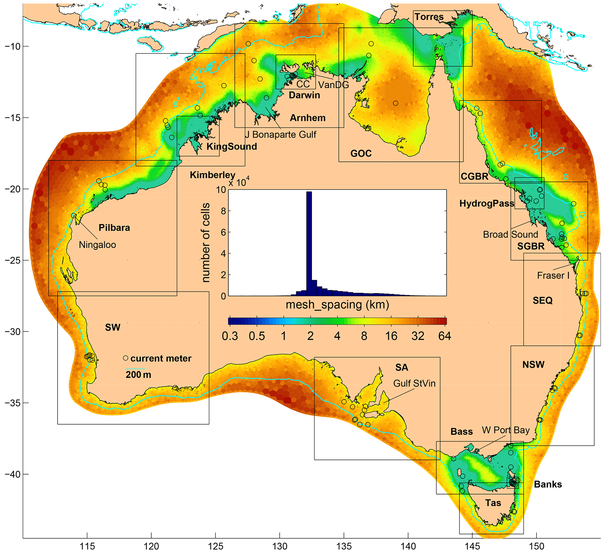
Figure 1Model mesh spacing (km, log scale). Abbreviated names are as follows. CC: Clarence Channel, VanDG: Van Diemen Gulf, GOC: Gulf of Carpentaria, CGBR: central Great Barrier Reef, SGBR: southern GBR, SEQ: southeastern Queensland, NSW: New South Wales, Bass: Bass Strait, Tas: Tasmania, Banks: Banks Strait, SA: South Australia, SW: the South West. The colour bar tick labels also apply to the bar graph above.
The model topography (Fig. 2) uses high-resolution datasets in the Great Barrier Reef (Beaman, 2010) and northern Australia (https://ecat.ga.gov.au/geonetwork/srv/eng/catalog.search#/metadata/121620, last access: 6 November 2020), supplemented with bathymetry from the Geosciences Australia (2002) database and the global database dbdb2 (Naval Research Laboratory Digital Bathymetry Data Base, https://www7320.nrlssc.navy.mil/DBDB2_WWW/, last access: 6 November 2020). Depth was median-filtered to remove sharp gradients. On-site depth measurements at the locations (Fig. 2) of the tidal current validation data discussed below were not used for estimating the model topography, thus providing a limited but independent validation dataset.
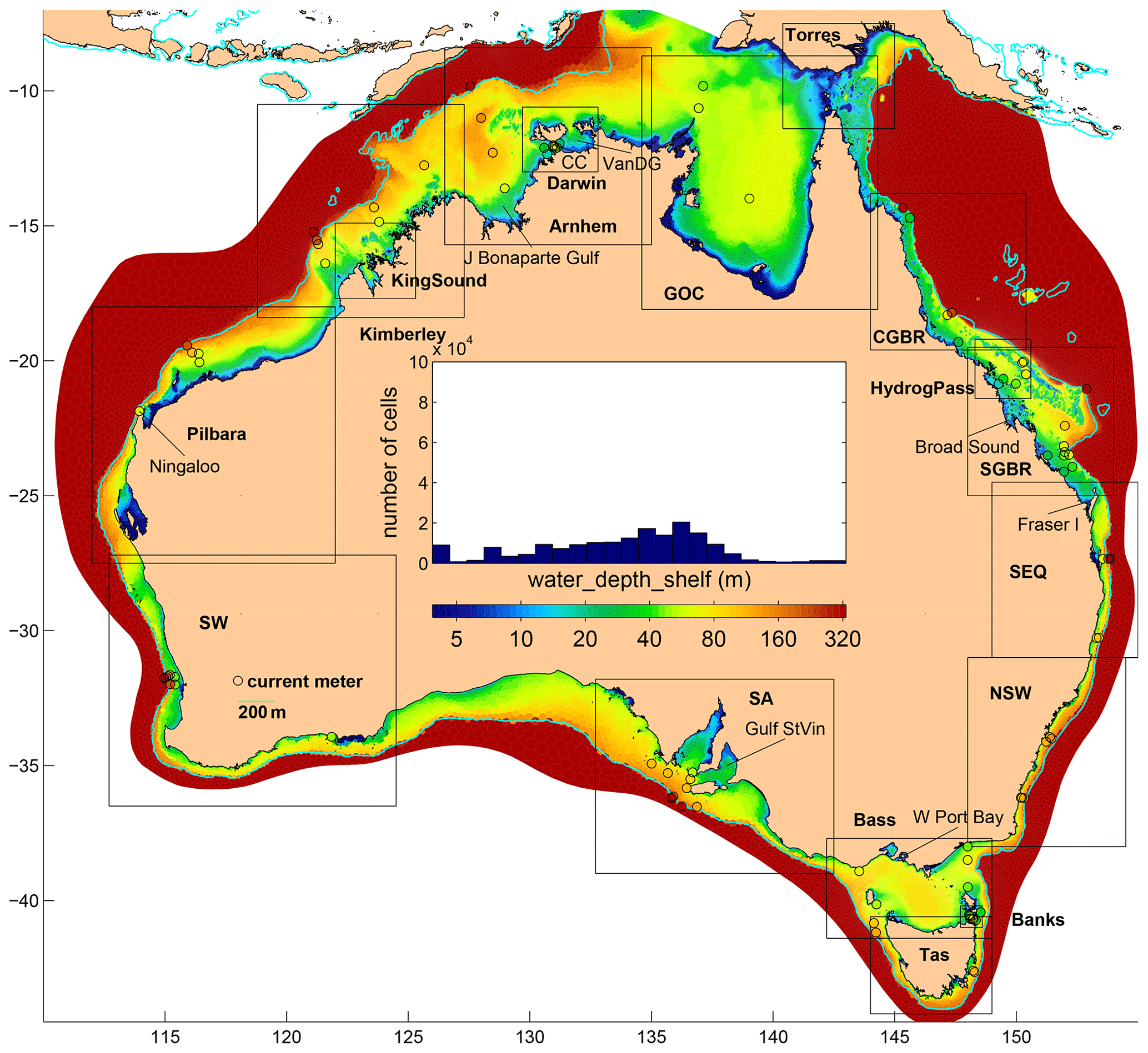
Figure 2Model depth (m, log scale, spanning just a restricted range); otherwise like Fig. 1.
COMPAS can be run with wetting and drying activated, not only for entire water columns, but also for individual layers (in a 3D application) as sea level falls or rises. For the present (2D) application, wetting and drying were not activated other than in preliminary test runs. The main problem with having wetting and drying activated was that it made comparison with tide gauges difficult. At many tide gauge sites, the model cells near the gauge dried at low tide but the observations showed that drying at the exact location of the tide gauge did not occur – presumably because the gauge is sited within a harbour or shipping channel unresolved by the model mesh. We chose to deal with this problem by preventing drying by setting the minimum depth (at zero tide) to 8 m at the coast in regions where the tides are large (impacting cells totalling 0.6 % of the total model area, mostly in the southern GBR and the region around Darwin) and 4 m elsewhere (impacting cells totalling 1.4 % of the model area, mostly in the Gulf of Carpentaria). The impact of this workaround solution on the nature of the tides, outside the impacted cells, was evidently negligible. A channel of 12 m was manually included in King Sound (in the NW) to correct an obvious error there, greatly improving the accuracy of the model in this location where Australia's greatest tides are to be found. A similar manual bathymetry correction was also made in Western Port (near Melbourne). We anticipate that further local improvements will follow from the use of an even finer mesh and a more complete set of observations of the real topography.
The tide is introduced through eight tidal constituents (M2, S2, N2, K2, K1, O1, P1, Q1) from the TPXO9v1 global model (Egbert and Erofeeva, 2002; https://www.tpxo.net/, last access: 6 November 2020) and applied at the open boundary using the condition described by Herzfeld et al. (2020a). The Herzfeld et al. (2020a) scheme includes a normal and tangential velocity Dirichlet condition with provision for a local flux adjustment on normal velocity to maintain domain-wide volume continuity. Thus, the surface height is not directly constrained at the boundary but is instead computed via volume flux divergence as it is in the model interior. For the present application, we found that flux adjustments to constrain the sea surface height were not required; prescribing the transports at the boundary was sufficient to achieve the target height. This situation is quite unusual and suggests that the TPXO values at the boundary are largely in tune with the interior dynamics of the model (even though TPXO and COMPAS have their differences), obviating the need for strategies to make the boundary transmissive to outgoing signals. One necessary step to achieve this was to use the TPXO components of transport on their native (Arakawa C) grid and use the depths in COMPAS to convert the transports to depth-averaged, cell-edge normal velocity, thus compensating for bathymetry differences between our model and the TPXO model. The model was run in 2D mode only using a time step of 1 s, achieving a runtime of on 12 processors. A spatially constant bottom drag coefficient of 0.003 was used to compute bottom stress. Tidal potential forcing as well as tidal self-attraction and loading (using the method of Sakamoto et al., 2013) are optionally applied in the model, but we found that it made very little difference (except the runtime) compared with other parameters such as friction, so we have omitted it for the long (1-year) run of the model described here.
For many test runs of the model, it was started from rest and run for either 7 or 30 d from 24 February 2017 including a 1 d ramp period. These trial model runs were too short for accurate decomposition into constituents, so we assessed them against height and velocity observations by harmonically synthesising (using T-Tide v1.3b; Pawlowicz et al., 2002) time series at all sites for which tidal constituents (up to 13) are available (see below). There are many more such sites than the number of observed time series available for any particular month, thus providing a more comprehensive assessment than would be possible by using only actual observed time series.
The model parameters adjusted during the series of test runs included (1) the bottom drag coefficient, (2) spatial variations of bottom drag, (3) bottom drag scheme, (4) coastal depth, (5) horizontal viscosity, (6) turbulence closure scheme, (7) bathymetry smoothing, (8) flux adjustment timescale, (9) tidal potential forcing on/off (left off finally), (10) bathymetry data source, and (11) interior relaxation to TPXO on/off (left off finally). These experiments proceeded in an ad hoc search for closer agreement with the observations. Apart from this “model tuning”, no data assimilation was used with these model runs.
For the model configuration described here, it was run for 365 d from 24 February 2017 and then tidally analysed for 13 constituents (M2, S2, N2, K2, K1, O1, P1, Q1, M4, MS4, M6, 2MS6, and 2N2) so that (1) its performance can be described for all those individual constituents and (2) predictions can be made for any time or place within the domain without having to run the model. The COMPAS model code, the output time series, and tidal constituents at all points of the mesh are freely available, as described in Sects. 9 and 10.
Acoustic Doppler current profilers (ADCPs) of various types have been deployed more than 1097 times as part of Australia's Integrated Marine Observing System (IMOS) at 55 sites over the continental shelf around Australia since 2007. The ADCPs are almost all moored within a few metres of the seabed and sense the water velocity over the lower 80 %–85 % of the water column. We have taken the depth average of these observations, concatenated all records from individual instrument deployments at the same nominal position, and determined the tidal constituents using the UTide software of Codiga (2011). A total of 13 constituents (M2, S2, N2, K2, K1, O1, P1, Q1, M4, MS4, M6, 2MS6, and 2N2) were analysed at the 64 sites having records exceeding 180 d. The records at other sites were all long enough to resolve 11 constituents (the full list minus K2 and P1). Apart from the deployments off the NW of the continent, these 55 IMOS sites tend to be at locations where tidal currents are not particularly strong. As a means of quantifying the relative magnitude of tidal and sub-tidal depth-averaged velocity, we determined the principal axis of the sub-tidal variability (using singular value decomposition) and computed the root mean square (rms) of the major and minor axis components. Details of the IMOS ADCP deployments are at http://oceancurrent.imos.org.au/timeseries/ (last access: 6 November 2020) along with regional graphics comparing the tidal and sub-tidal ellipse parameters (as well as the mean velocity for each deployment).
Penesis et al. (2020) give details of ADCP deployments that deliberately sought to observe tidal currents for two of Australia's most prospective tidal energy development regions. These include seven locations in the Clarence Channel near Darwin and seven locations in Banks Strait at the NE tip of Tasmania. We determined tidal velocity constituents, the mean, and sub-tidal ellipse parameters from these data as above.
We have included data from 10 of the sites where Middleton et al. (1984) and Griffin et al. (1987) deployed current meters on the southern Great Barrier Reef (SGBR, see Fig. 2) in order to study both the anomalous tides and the sub-tidal variability. These observations were made by single mechanical RCM4 Aanderaa current meters with several drawbacks compared to ADCPs. Due to limited storage capacity, the flow direction was only sampled instantaneously once an hour, so short-period changes of direction were not averaged. To minimise noise due to waves (i.e. rectified orbital velocities spinning the rotor even when the current velocity is zero – Griffin, 1988), the instruments were moored fairly low in the water column (typically 7 m off the seabed), thereby probably underestimating the depth-averaged velocity. Some had to be deployed close to islands, with the result that they recorded effects (such as asymmetric ebb and flood directions) that the model is unlikely to be able to reproduce at specific locations due to its imperfect representation of topography. Nevertheless, we have included these records in our validation dataset, processed as above, despite the quality questions because (1) the tides in this region are important for navigation (e.g. through Hydrographers Passage) and (2) in the hope that future models with finer meshes and better topography may be able to better distinguish observation error from model error.
Lastly, we also extracted 13 current meter records from the CSIRO archives (https://www.cmar.csiro.au/data/trawler/, last access: 6 November 2020), choosing sites in Bass Strait, the NW shelf, and the Gulf of Carpentaria where tidal currents are significant. These were mostly point measurements, either by acoustic or mechanical (Aanderaa) current meters. Where two instruments were deployed on a mooring, we simply averaged the data for the period when both were operating.
In support of this paper and future studies of the tides of Australia, we have published this validation dataset as a NetCDF file containing up to 13 tidal constituents and the sub-tidal statistics for each of the 95 locations discussed above (see Sect. 10).
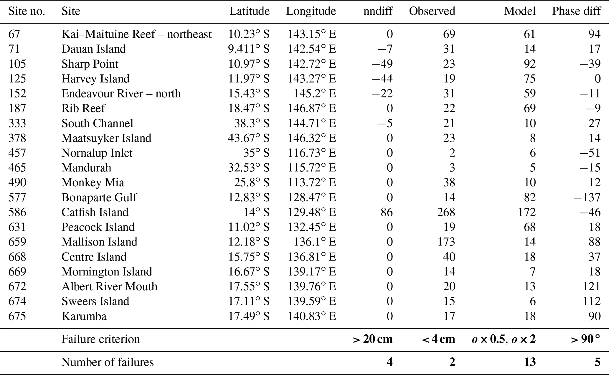
Table 1Blacklisted tide gauges. Tests are on the nearest-neighbour difference (cm), the observed M2 amplitude (cm), and the model M2 amplitude (cm) and phase relative to the observed values. Failure criteria for these tests and the number of sites failing the tests are given at the bottom of the table.
The National Operations Centre (NOC) Tidal Unit of the Bureau of Meteorology (http://www.bom.gov.au/oceanography/projects/ntc/ntc.shtml, last access: 6 November 2020) kindly provided eight tidal height constituents (M2, S2, N2, K2, K1, O1, P1, Q1) for 683 sites, 626 of which are within the COMPAS domain. To this we have added nine sites from the UNSW SGBR dataset, bringing the total to 635 before applying quality control.
The model–data comparisons presented in this paper are based on the tidal constituents (M2, S2, N2, K2, K1, O1, P1, Q1) determined from the model and observational time series (rather than the time series approach used during model tuning) for all the usual reasons, some of which are (1) the nature of model (and observation) errors is likely to differ significantly depending on the constituent frequency and amplitude, (2) errors of the ellipse orientation are then easily distinguished from errors of the phase and major axis length, all of which differently impact various users, and (3) it is the most succinct way of describing the dataset. We focus on results for M2, or sums over the eight major constituents. Availability of the full set of model–data comparisons for 13 constituents, 18 regions, and 5 variables is covered in Sect. 10.
5.1 Tide gauges
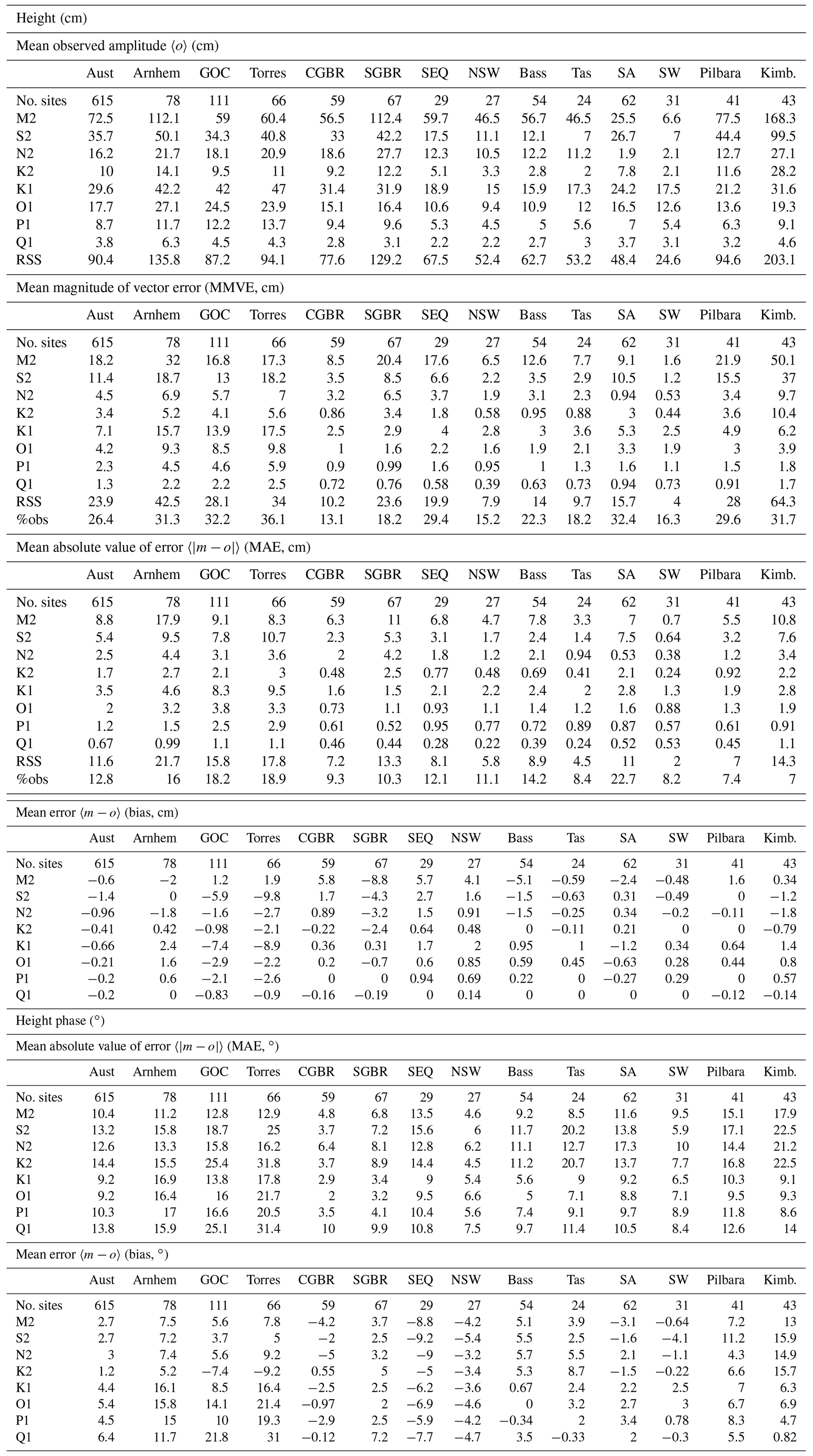
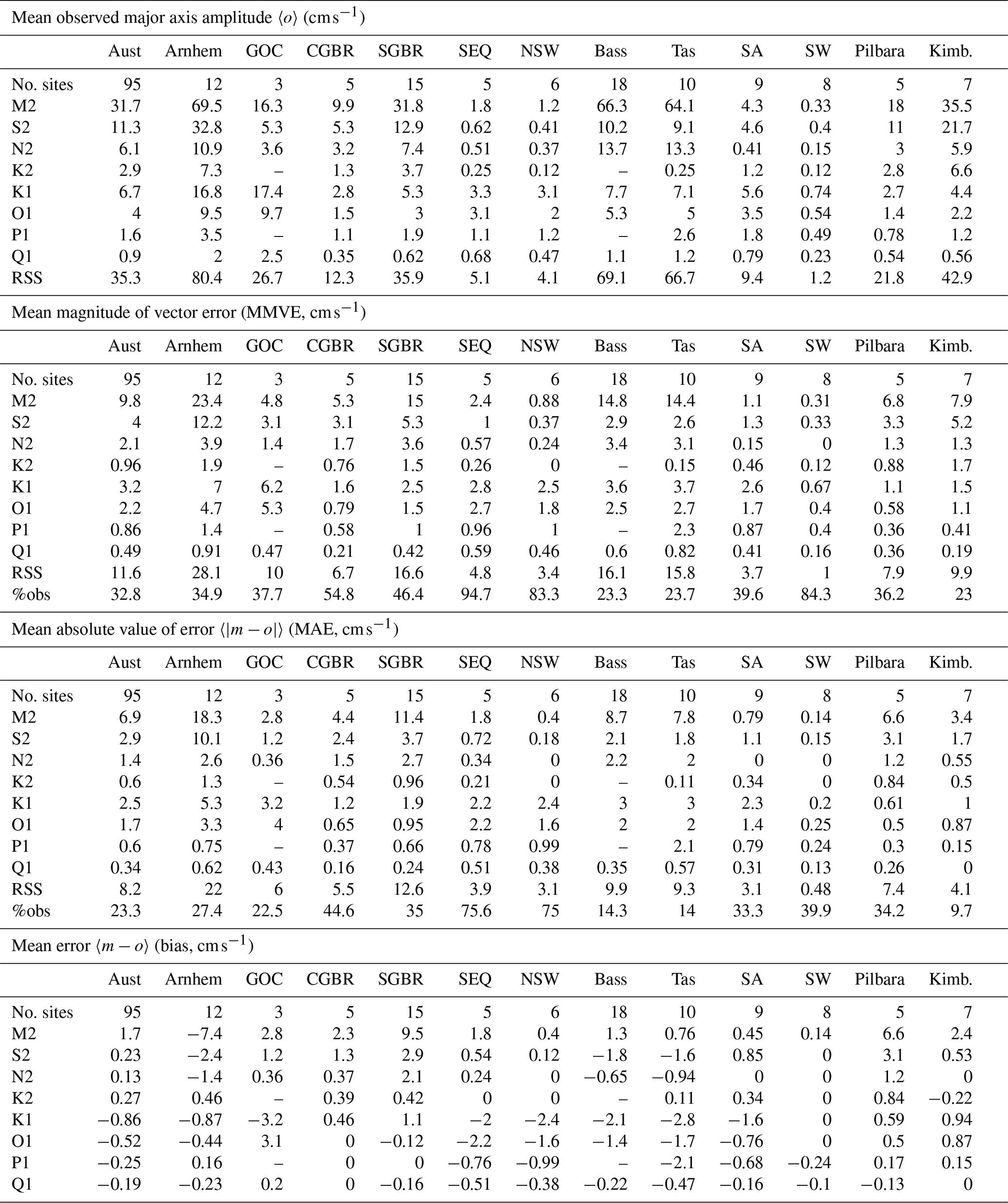
When comparing the model with tide gauges, we select the closest model grid point if one exists within 11 km. We calculate the model error (model minus observation) for amplitude and phase individually as well as the vector error (taking both phase and amplitude into account) for each tidal constituent. Summing over a number of sites within a certain geographic region, we then compute the mean of the absolute value of the amplitude error (MAE), the mean magnitude of vector error (MMVE), the mean of the amplitude error, and the mean of the observed amplitude (for expressing the MAE or MMVE as a relative error or RE). We use MAE and MMVE in preference to root mean squared errors because the MAE and MMVE are less affected by outliers. Outliers are a significant issue, as we will discuss below with reference to Table 1, which lists the sites we have chosen to exclude from the tidal height dataset. We combine analyses across constituents by computing the root sum of squared (RSS) MAEs and MMVEs. In order to estimate the total regional-mean tidal relative error, we also compute the RSS of the area-mean observed amplitudes. These statistics are computed for a number of regions (bounding boxes are shown in Fig. 1) around Australia as well as for the entire country and listed in Table 2. We have not attempted to account for the uneven distribution of the data points around Australia, other than to compute regional means and nationwide means. Nor have we attempted to estimate errors of the observational tidal constituents based on factors such as record length or instrument type, these being unknown in many cases.
Table 2Tidal height and phase regionally averaged statistics for eight constituents (and their root sum of squares – RSS). The %obs row expresses the RSS values in the line above as a percentage of the observed RSS.
5.2 Current meters
When comparing with current meters, we select the grid point for which a penalty function is minimised, where D is the distance (km) to the model grid point, C is the characteristic size (km) of the cell (see Fig. 1), Hm is the model depth, and Ho is the on-site depth at the observation point. This is an attempt to mitigate the effect of the model's imperfect topography by finding the nearest depth-matching (if possible) model counterpart of the observation. We then proceed as for tide gauges, but with the amplitude and phase of the major axis velocity taking the place of height. Errors of the major axis inclination and minor axis amplitude are shown graphically and are listed in Table 3 but are not otherwise included. Three sorts of site-specific relative error are listed in Table 3: (1) the M2 major axis velocity amplitude error relative to the observed amplitude , (2) the M2 major axis velocity vector error relative to the observed amplitude , and (3) , which takes the observed sub-tidal (“low-frequency”) rms major axis velocity subo into account. The first two measures characterise the model's ability to do what it is designed for, which is just to simulate tides. The first of these is for users who need to know tidal range but not at any particular time. The second is for applications for which timing is also important. The third acknowledges that tides are not the dominant component of velocity variability everywhere. Using a tidal model alone (i.e. without a model of other processes) to predict the total current (characterised by majo+subo) will result in an error determined by subo if the tidal error is zero. Where tidal variability and sub-tidal variability are equal, the upper limit of reLF is 50 %.
Table 3Model errors at current meter sites – M2 constituent. The columns are current meter site name and location, then three measures of the observed, depth-averaged, non-tidal velocity: |mean|, dir, and subo, which are the magnitude and (compass) direction of the mean and the magnitude of the root mean square of the sub-tidal low-pass-filtered velocity. Next are the observed (_o) and model (_m) values of depth h, M2 major axis inclination (inc), and minor and major axis amplitudes (min and maj). Next are the errors majm−majo and gm−go (m−o for short) of the major axis amplitude and Greenwich phase g, then the magnitude of the vector (amplitude and phase) error . Next are three types of M2 percentage relative errors: reM2 , re, and sub subo). Sites are listed by ascending reLF. The means (over successive thirds of the dataset (e.g. after row 32), and then for all of it) of the absolute value of some quantities are given. Note that observed inclination angles are chosen to be −90 to 90∘ T. Listed model inclinations and Greenwich phases are both flipped 180∘ in a few sensible instances.

Table 3 lists sites by ascending reLF and includes averages of the sites with the lowest, middle, and greatest reLF for most columns. For the m−o column the average is mathematically an MAE, but with a non-geographic sample of sites. Table 4 is like Table 2, with major axis velocity amplitude and phase taking the place of height amplitude and phase, for the same eight constituents.
Table 4Tidal major axis velocity and phase regionally averaged statistics for eight constituents (and their root sum of squares).
6.1 Tidal height
Since we have no reliable, objective (model-independent) way of knowing which tide gauge observations (or more precisely, the analysed tidal constituents) are more accurate than others, we have cautiously employed a largely model-based quality control procedure. This procedure excludes sites if
-
the absolute value of M2 error exceeds 20 cm and an observed M2 amplitude within 10 km is less by more than 20 cm (excludes four sites),
-
the observed amplitude is less than 4 cm (two sites),
-
the observed amplitude exceeds 10 cm and is less than half or more than twice the model amplitude (14 sites), and/or
-
the observed and modelled phases differ by more than 90∘ (six sites).
With the 20 sites listed in Table 1 excluded, the M2 MAE across 615 sites is 8.8 cm (Table 2), or 12 % of the mean observed amplitude, which is 72.5 cm. The resulting scatter plot (Fig. 3, note the log–log axes) of model vs. observed height amplitude still has points that could be considered outliers; at 5 % of sites the negative errors are ∼3 to 10 times the MAE. But we have not excluded these along with the other 20 for lack of clear evidence that they are due to observation error rather than model error.
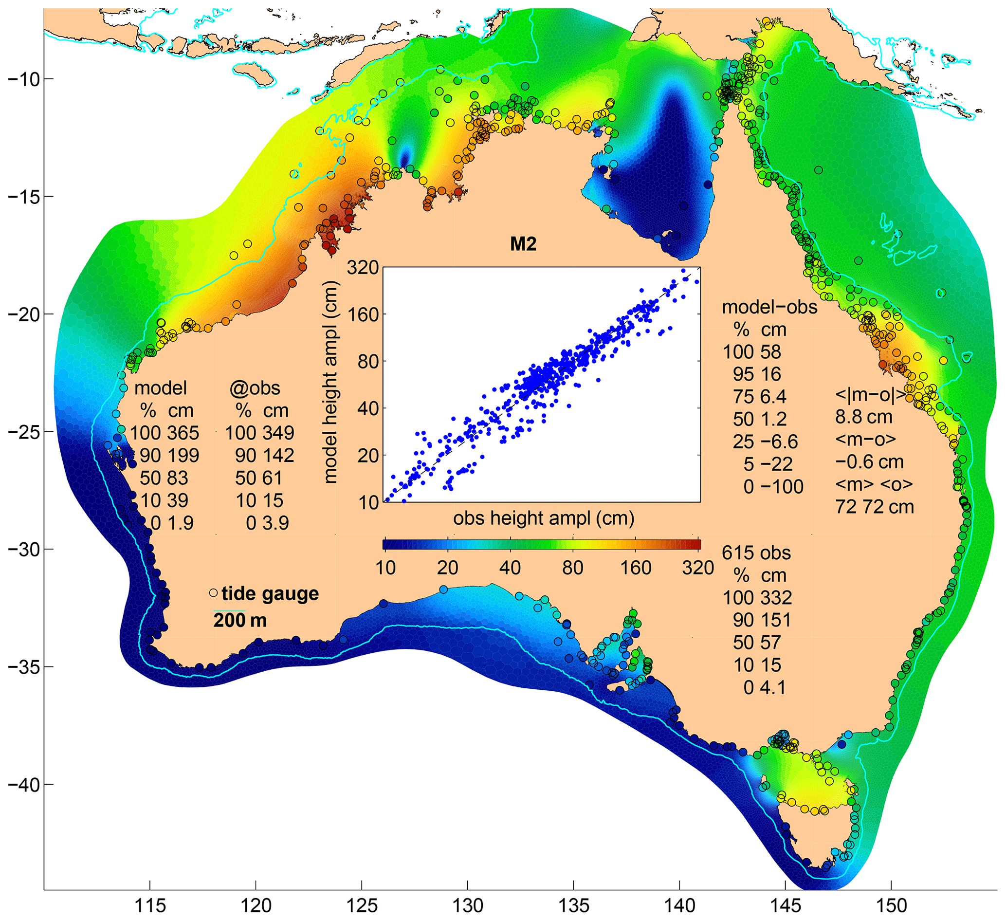
Figure 3M2 height amplitude as a colour-fill map (the model) and points (observations); inset as a quantity–quantity plot. Statistics listed are percentiles (% columns) of (1) the model height field at all grid points (“model” column at left), (2) the model at observation sites, hereafter m (“@ obs” column), (3) model error (“model-obs” column), and (4) the observed values o of which there are 615 within the area shown (“615 obs” column). At far right the following are listed: , the mean of the absolute value of m−o; 〈m−o〉, the mean error, or bias; and 〈m〉 and 〈o〉, the mean modelled and observed amplitudes. A log scale is used, starting at 10 cm, so not all points can be shown.
The nationwide bias is small (−0.6 cm, see Table 2), but some regional biases are not. The region with the biggest M2 bias (−8.8 cm) is clearly (see Table 2) the southern Great Barrier Reef, where the model underpredicts the large tides within about 100 km of the head of Broad Sound
The region with the biggest M2 amplitude MAE (at 17.9 cm) is the one we abbreviate here as “Arnhem” (rather than Joseph Bonaparte Gulf and Arnhem Land), but across this region there is a mix of underprediction and overprediction. The modelled M2 height amplitude is too small in Van Diemen Gulf and the head of Joseph Bonaparte Gulf but too great at many of the offshore sites where the observed amplitude is small.
There are large M2 phase errors (Fig. 4) at many sites. While some are possibly due to observation error, the predominance of positive phase errors at locations of strong tides points to a problem in the model. The region with the biggest M2 phase MAE is the Kimberley (18∘) (Table 2), which is nearly twice the all-site average of 10.4∘. The significant phase errors are why the Australia-wide M2 MMVE (18.2 cm) is so much greater than the M2 MAE (8.8 cm).
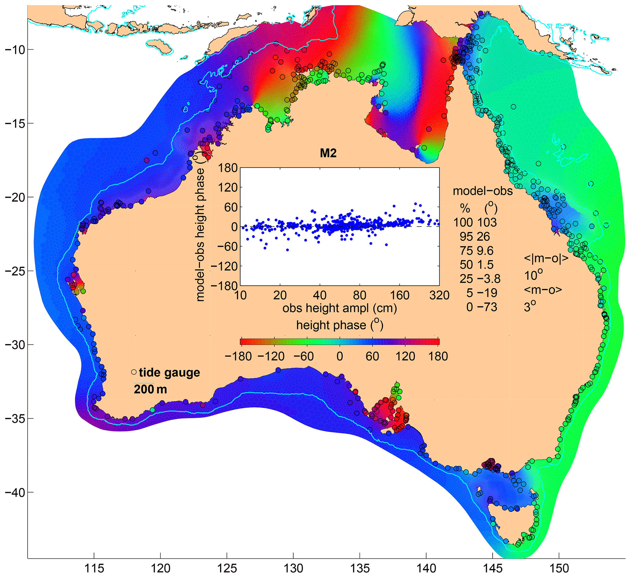
Figure 4M2 height phase (otherwise like Fig. 3, except the y axis of the inset is the phase error rather than phase).
The next most energetic constituent after M2 (72.5 cm averaged across all sites) is S2 (35.7 cm). S2 has the next-greatest MMVE (11.4 cm, because of large phase errors in the Kimberley).
Summing over eight constituents and taking both phase and amplitude errors into account, the RSS MMVE across all sites is 23.9 cm, or 26.4 % of the mean observed amplitude. The three regions with the lowest relative error (13 %, 15 %, and 16 %) are the central Great Barrier Reef, New South Wales, and the South West, while the regions with the highest (31 %–36 %) are South Australia, the wide shallow seas in the tropics (Torres Strait, Joseph Bonaparte Gulf, and Arnhem Land), the Kimberley, and the Gulf of Carpentaria. Thus, the greatest regionally averaged relative errors of modelled height are about twice the size of the least. Both are small enough to conclude that the model has skill but large enough to conclude that there is still room for improvement.
6.2 Tidal currents
Perhaps the most striking difference between maps of the M2 major axis amplitude (Fig. 5) and the M2 height amplitude (Fig. 3) is that the currents have more small-scale variability, clearly associated with the local topography, as well as regional variability that broadly reflects the regional variations of tidal range. Characterising and analysing the distribution of the errors as well as the signal are not straightforward but are what we will attempt to do after looking at some of the site-specific results listed in Table 3.
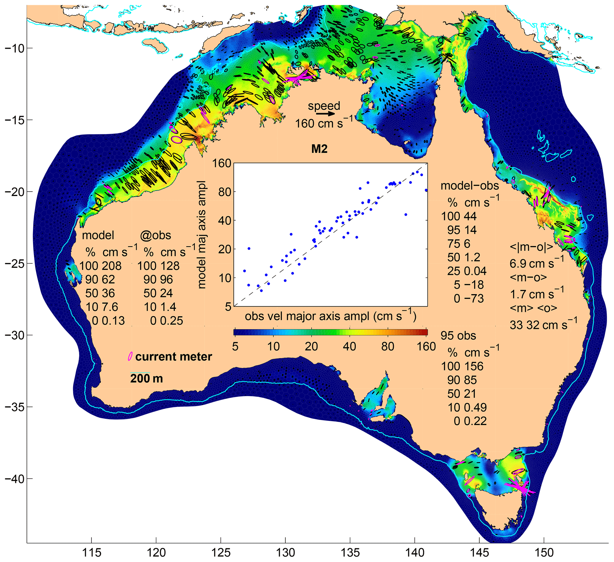
Figure 5Amplitude of the M2 major axis velocity; otherwise like Fig. 3. Black (model, at a random subset of grid points) and magenta (observed) velocity ellipses use the scale shown.
The first line of Table 3 is for the IMOS site north of Heron Island in the southern Great Barrier Reef. It is the first line because it has the lowest reLF, which in turn is because the errors of the M2 major axis velocity phase and amplitude are both small (−1∘ and −3 cm s−1), while the amplitude of the observed M2 tidal currents is large (50 cm s−1) compared to the rms sub-tidal velocity (8 cm s−1). Site CW3 (line 3) sampled by Penesis et al. (2020) in Banks Strait is a more energetic site, but the errors of the major axis velocity phase and amplitude are both relatively small (9∘ and 1 cm s−1) nevertheless. It is also a tidally dominated site (98 cm s−1 for M2 compared to the sub-tidal velocity of just 7 cm s−1). As it happens, the error of the minor axis is also very small (both are essentially zero) here, but the error of the inclination is not (−28∘ T observed but −52∘ T modelled). Site CW1 (line 6) is about 3 km away (just one grid cell) and has a greater amplitude error (14 cm s−1) but less inclination error (2∘). Looking down the table we see that 8 of the 18 lowest-error sites are in Banks Strait. This is clearly a region where the model in its present form is capable of producing current velocity predictions with low relative error, so it is the first to be discussed in the next section.
At the other extreme (at the bottom of Table 3) is GBRLSL, a site off the Great Barrier Reef in 330 m of water where the observed M2 major axis velocity is essentially zero, but the model estimate is 7 cm s−1. Second-bottom is NRSNIN, an IMOS ADCP at the Ningaloo Reef National Reference Site in Western Australia, where the observed M2 major axis amplitude is just 7 cm s−1, while the model estimate is 20 cm s−1. From the prediction point of view, the errors at these two sites are compounded by there being fairly strong (12 and 18 cm s−1) sub-tidal currents but small mean current (4 cm s−1). One thing these two sites have in common is that they are over steep topography where sharp gradients are common, so part of the poor agreement is bound to be due to representation error (the error that occurs when you compare a point measurement with an area average). But even so, these are probably not sites where tidal predictions will be of much practical use.
Table 3 includes statistics that characterise model error averaged over sites grouped according to whether reLF is in the lowest, middle, or highest third. The MAE over this first third is 7 cm s−1 (an 11 % average relative error), while the MMVE is 14 cm s−1, a 21 % average relative error or 29 % if sub-tidal currents are taken into account as well. For the locations that these sites are representative of, you could argue that the tidal model is not only useful, but is also enough by itself; i.e. a short-term forecast of sub-tidal current velocity would not often make a significant contribution (since its mean rms value is around 6 cm s−1, just 10 % of the mean M2 amplitude). For the middle group the average M2 tidal current amplitude (27 cm s−1) alone still exceeds the sub-tidal variability (10 cm s−1), but the dominance is less than for the first third, and the errors (MMVE = 12 cm s−1) of the tidal model are not insignificant. The average reLF for this group is 59 %, which could be argued as being acceptable but with much room for reduction, either by improvements to the tidal model or addition in near-real time of a skilful forecast of sub-tidal variability. For the final third, the observed tidal currents are mostly insignificant (3 cm s−1 compared to 22 cm s−1), so it does not really matter what the predicted tidal velocity is, as long as it is weak. This last group includes all 11 sites in the New South Wales and southeastern Queensland regions, 5 of the deeper (∼100 m or more) sites in South Australia, and all 8 of the sites in southwest Western Australia. We will now look more closely at the regions where tidal currents are a large fraction of the variability.
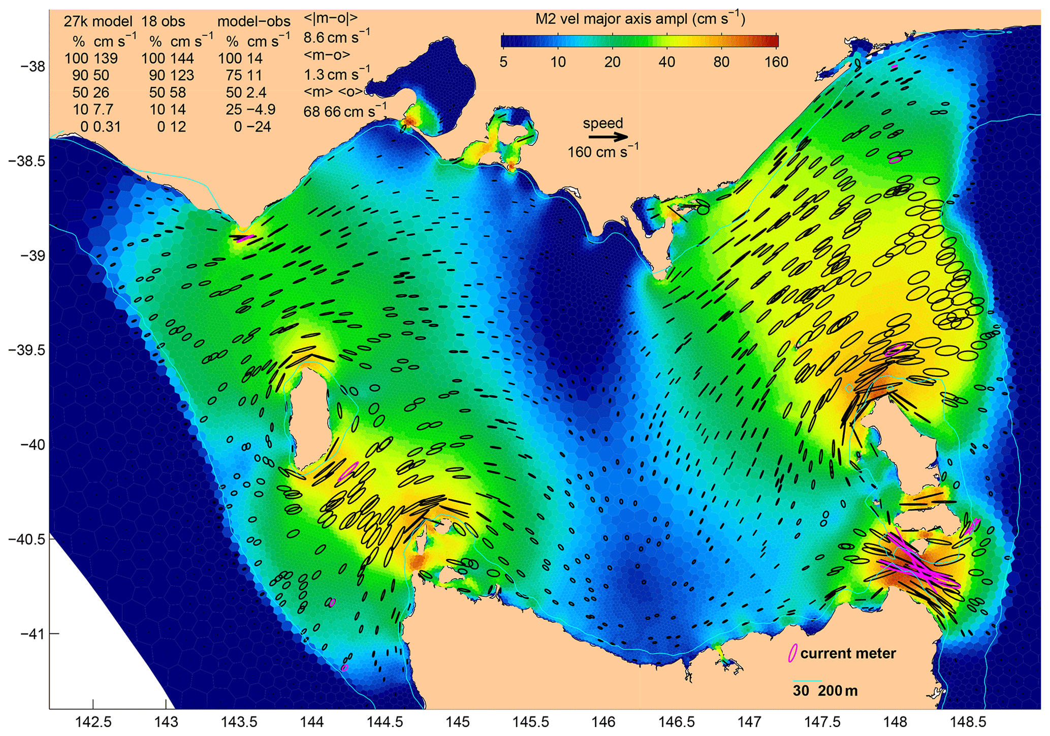
Figure 6Amplitude of the M2 major axis velocity for Bass Strait; otherwise like Fig. 5, except that percentiles of the model at the locations of the observations are not listed.
6.2.1 Bass Strait (including Banks Strait)
The tide comes into Bass Strait from both the east and west, with the strongest flows (Fig. 6) either side of the central basin (see Fig. 2) where the tidal range (Fig. 3) is maximum. The highest tidal ranges are near Burnie on the northern Tasmanian coast. Recalling that tidal potential forcing is not activated in this run of the model, the agreement of our model with the observations is in contrast with the conclusion by Wijeratne et al. (2012) that tidal potential forcing is required for a nested model of Bass Strait to be accurate. We offer no explanation for this inconsistency. The greatest observed M2 major axis amplitude is 144 cm s−1 (at C1A3 in Banks Strait – see Fig. 7 – one of the Penesis et al., 2020, ADCPs), while the model estimate is 120 cm s−1 (line 16 of Table 3). This is also the biggest error in Bass Strait, but it is still quite a small (−17 %) relative error of amplitude. Taking the phase error also into account takes this to 26 %. Table 4 lists the M2 MAE across the 18 validation sites in Bass Strait as 8.7 cm s−1. The RSS across eight constituents is 9.9 cm s−1, or 14.3 % of the 69 cm s−1 mean observed RSS of amplitudes – a much better than average (23 % across Australia) relative error. Figure 6 and Table 3 show that, across Bass Strait, the modelled M2 current ellipse eccentricities and orientations are mostly in good agreement with observations. The phase errors range from −9 to 12∘. Summing over eight constituents and taking the phase errors into account (Table 4), the RSS MMVE is 16.1 cm s−1, or 23.3 % of the mean observed RSS amplitude, making Bass Strait one of the two regions with the lowest (with the Kimberley) relative error of RSS MMVE. See below for a discussion of the M4 constituent.
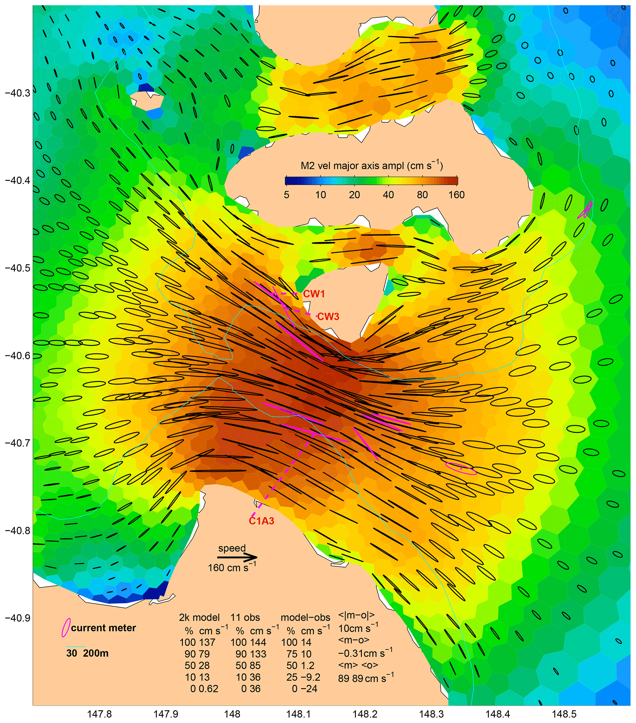
Figure 7Amplitude of the M2 major axis velocity for Banks Strait; otherwise like Fig. 5.
6.2.2 Kimberley
The Kimberley region of Australia includes King Sound, where the greatest tidal range in Australia occurs. The entrance to King Sound has such strong tidal currents that tourists go out to see them in speedboats, helicopters, and other vessels. There are not, however, any available instrumental records of the flows in the most energetic regions, so the percentiles of the model (across ∼30 000 cells; see Fig. 8) are very different to the percentiles of the observations. Figure 8 shows that the model agrees quite well with the seven available records, including the change from nearly circular M2 ellipses at KIM050 to the shore-normal rectilinear flows at CAM050 and CAM100, and then the weak shore-parallel ellipses at TIMORS88. The M2 amplitude errors at KIM100 and KIM200 are just 3 % and −1 % of the observed amplitude. It is only with the phase taken into account that the M2 relative errors are significant (11 % and 1 %). The RSS MMVE is 9.9 cm s−1, or 23 % of the observed RSS amplitude, like the Bass Strait figure.
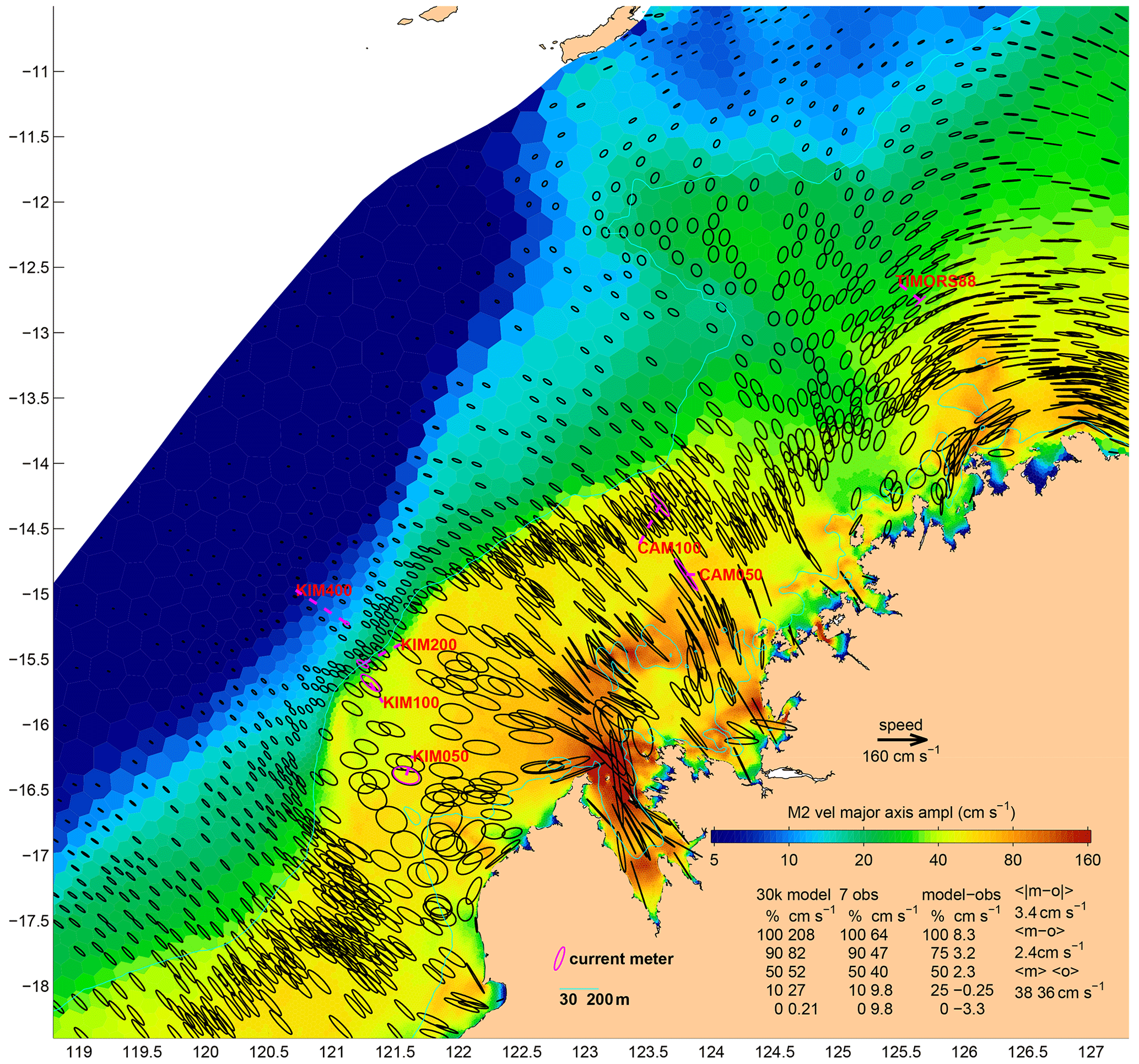
Figure 8Amplitude of the M2 major axis velocity for the Kimberley; otherwise like Fig. 5.
6.2.3 Darwin
Figure 9 shows that M2 velocity errors are relatively low at six of the eight sites in the Darwin–Clarence Channel region. Table 3 (lines 42 and 50) identifies the two noticeable exceptions as being the Darwin C1 and CW1 sites, where the M2 major axis amplitude errors are −73 and −63 cm s−1. At C1 the problem is clearly the topography; model depth is only 30 m, but the in situ depth is 52 m. It is less clear why the error at CW1 is large, but we will not be surprised if rebuilding the mesh using recently acquired topography data does not reduce these errors. At present, however, the velocity major axis RSS MMVE for Arnhem remains listed as 28.1 cm s−1, or 34.9 % of the observed RSS amplitude. The modelled tidal height amplitude in Van Diemen Gulf (Fig. 10) is significantly weaker than the observations for reasons that we have yet to determine.
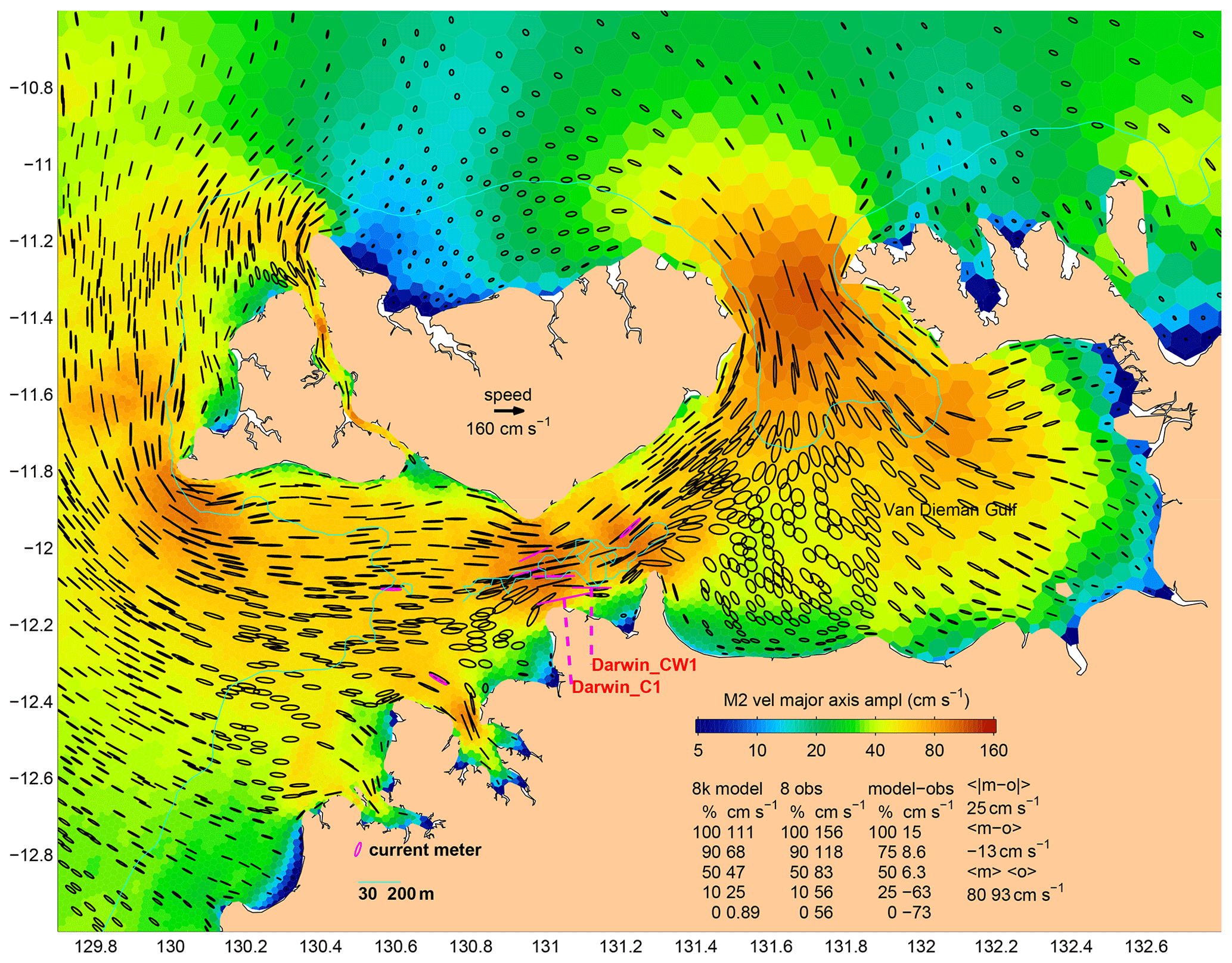
Figure 9Amplitude of the M2 major axis velocity for the Darwin region; otherwise like Fig. 5.
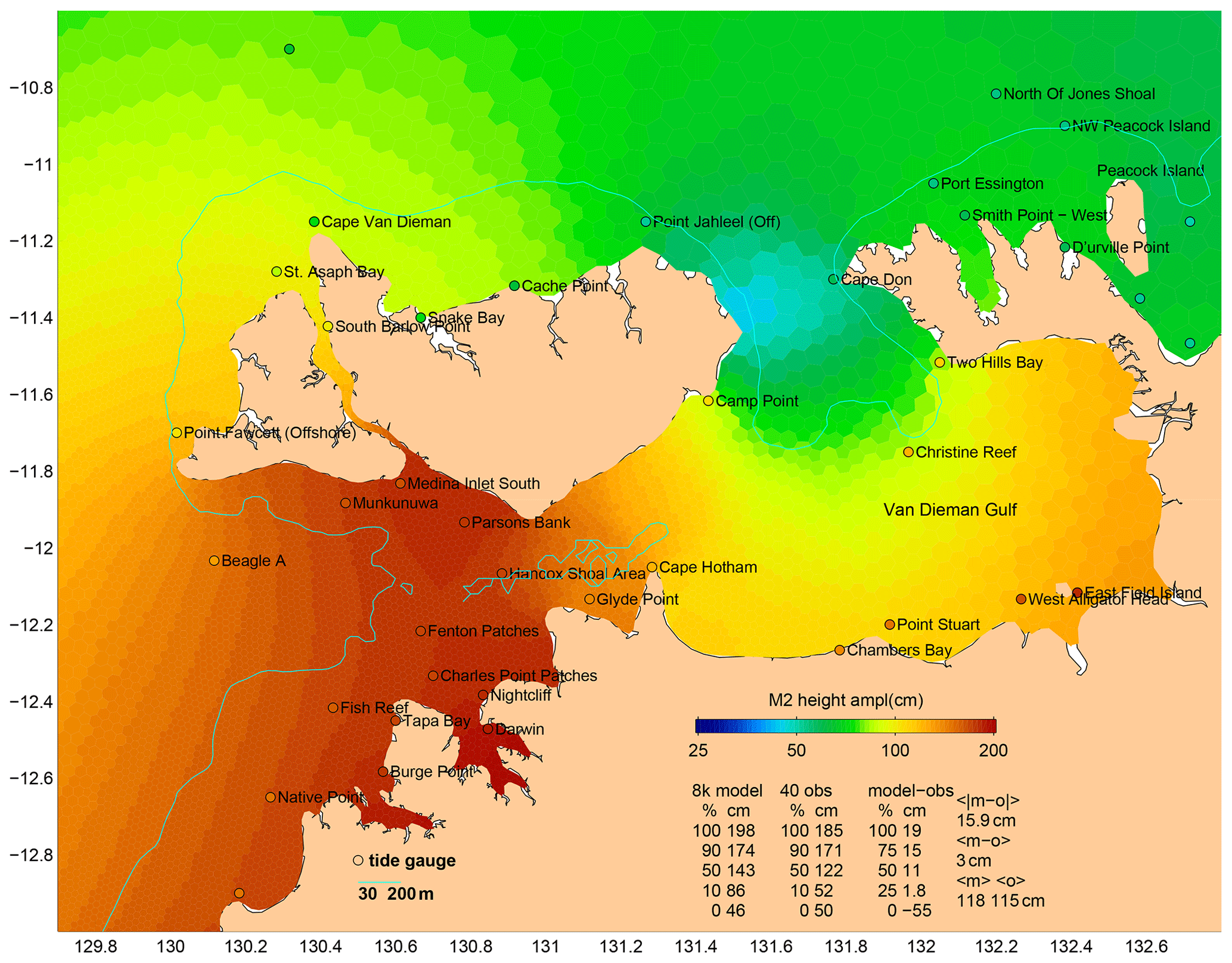
Figure 10Amplitude of the M2 height for the Darwin region; otherwise like Fig. 3.
6.2.4 Southern Great Barrier Reef
The Barrier Reef is dense off Broad Sound, causing tides to enter the reef lagoon from both the NW and SE. These waves meet in the lagoon outside Broad Sound, and then further amplification of the wave entering the sound occurs due to the geometry of the sound (Middleton, Buchwald, and Huthnance, 1984). Our model simulates the first process satisfactorily in a qualitative sense (see Fig. 11), and the modelled and observed tidal currents are in very good agreement at many locations. But Table 4 also lists some large discrepancies at several sites. These are where the observations were made by mechanical current meters, some in topographically complex locations (two near Bugatti Reef, one near Lady Musgrave Island), so the listed RSS MMVE of 16.6 cm s−1 (or 46.4 % of the observed amplitude) possibly overstates the true error. The tide gauge (at McEwin Islet) near the head of the sound (Fig. 12) suggests that the second amplification process is also quite well modelled, since the modelled M2 amplitude there is nearly (within about 10 %) as great as the observed value.

Figure 11Amplitude of the M2 major axis velocity for the southern Great Barrier Reef region; otherwise like Fig. 5.
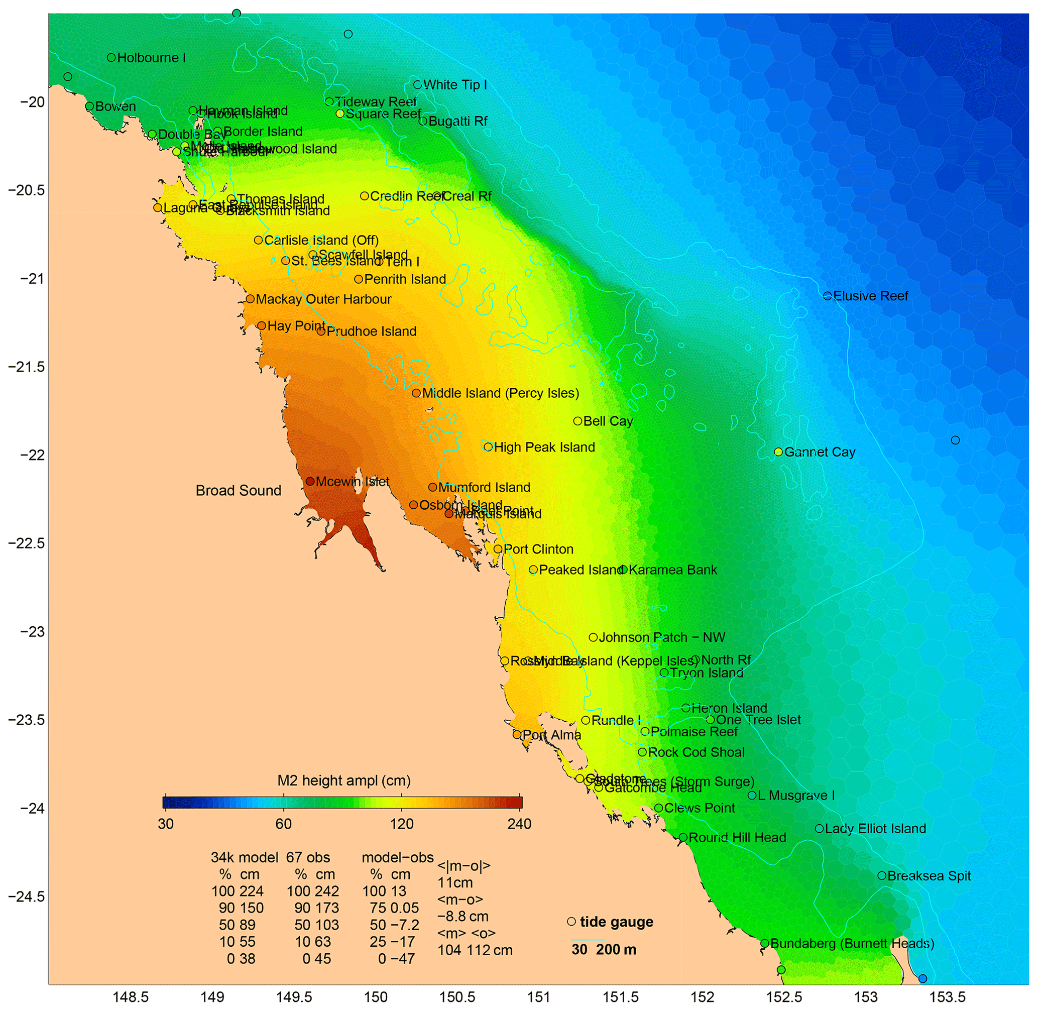
Figure 12Amplitude of the M2 height for the southern Great Barrier Reef region; otherwise like Fig. 3.
6.2.5 South Australia
A distinctive feature of the tides of South Australia is that the amplitudes of S2 and M2 are nearly the same, leading to a very strong spring–neap cycle. The vanishing semidiurnal tide on days when M2 and S2 are out of phase is locally known as the dodge tide. Table 2 lists the SA-average observed M2 and S2 height and major axis amplitudes as 25.5 and 26.7 cm and as 4.3 and 4.6 cm s−1. The model M2 and S2 height and major axis amplitudes (not listed) are also nearly equal at 23 and 27 cm and at 4.7 and 5.4 cm s−1 so dodge tides will also occur (imperfectly) in model-generated predictions. The maximum modelled M2 major axis amplitude is 41 cm s−1 in the South Australian region (Fig. 13), but we have no observations to validate the model at that location. The maximum observed M2 major axis amplitude is 9 cm s−1 at both SAM6IS and SAM8SG (rows 41 and 55 of Table 3) where the model is in very close and good agreement, respectively. The RSS MMVE for SA is 3.7 cm s−1, or 39.6 % of the observed amplitude.
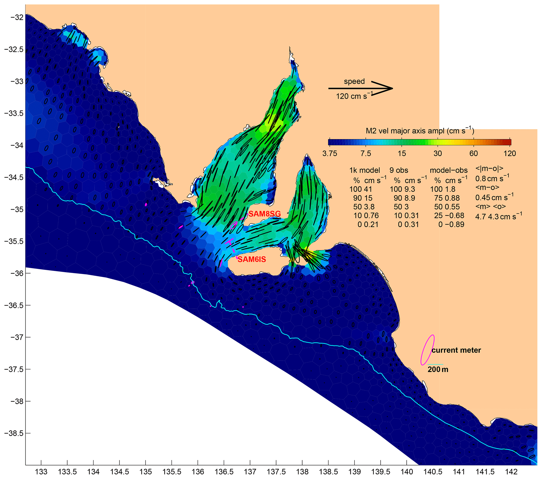
Figure 13Amplitude of the M2 major axis velocity for the South Australia region; otherwise like Fig. 5.
6.2.6 Pilbara
Table 3 lists results for just five sites in the Pilbara region (one being the Ningaloo site mentioned earlier as having the greatest error). Unfortunately, these are all we have in our validation dataset despite the economic importance of marine traffic in this region. Results for the three IMOS ADCPs near 20∘ S (PIL050, 100 and 200) include M2 vector errors of 15 % to 26 % of the observed amplitude. But this region is well known for strong internal tides (Book et al., 2016), to which our analysis method is essentially blind. Internal tides aside, the RSS MMVE for this region is 7.9 cm s−1, or 36.2 % of the observed amplitude.
6.2.7 Gulf of Carpentaria, Torres Strait, central Great Barrier Reef
The GOC and CGBR regions have intermediate (37.7 % and 54.8 %) relative errors of the RSS MMVE, but being based on just three and five sites, these statistics are uncertain. Nevertheless, we see value in publishing tidal current predictions for these two regions with appropriate warnings, partly because the sub-tidal currents are weak in these two regions. As mentioned earlier, Torres Strait is one of the few places where official tidal current predictions are already published. We have not yet compared those predictions or observation-based constituents with our model.
6.2.8 Southeastern Queensland, New South Wales, and the South West
The relative error of the RSS MMVE for the SEQ, NSW, and SW regions are 95 %, 83 %, and 84 %, respectively, suggesting that the model is not simulating the tidal currents in these regions very well, even though it is simulating the heights (recall that NSW is one of the regions with the lowest relative error of height). It appears that this problem is largely inherited from the boundary conditions. These narrow-shelf regions are also where the sub-tidal currents (Table 3) far exceed the tidal currents, so predictions of tidal currents would be of limited practical value even if they were accurate. For both these reasons, we will not be publishing tidal current predictions from the COMPAS model for these regions.
6.2.9 High-frequency constituents
As mentioned in Sects. 2 and 3, we have analysed both the model and the velocity validation dataset for 13 tidal constituents. Table 4 does not include results for M4, MS4, M6, 2MS6, or 2N2 because the amplitudes are mostly insignificant. An exception is the M4 constituent in Banks Strait, where amplitudes up to 5.9 cm s−1 were observed (Fig. 14). Model amplitudes are comparable (up to 4.3 cm s−1), but there is not much correspondence with the observations. Given the complexity of both the observed and the modelled currents, as well as the relatively small contribution to the total, we cannot be confident that the modelled M4 velocities are accurate enough to warrant inclusion of these constituents when making predictions.
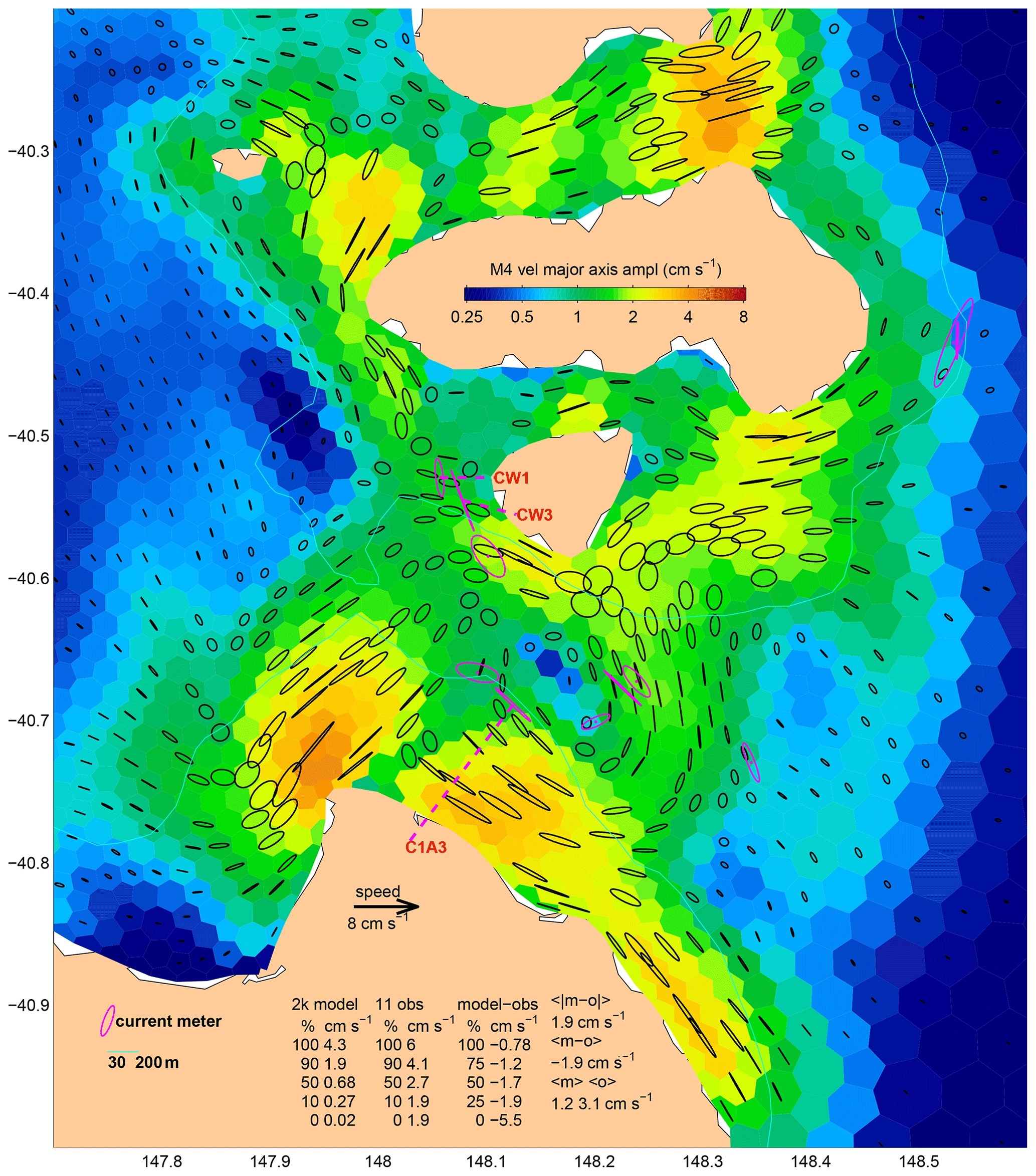
Figure 14Amplitude of the M4 major axis velocity for the Banks Strait region; otherwise like Fig. 5.
We have evaluated the tidal heights in our COMPAS model against a large number (615) of sites around Australia, giving a much more detailed picture than was given, for example, by Haigh et al. (2014) or Seifi et al. (2019), while being broadly consistent. But modelling tidal heights is not the principal motivation of this study. Our focus is on tidal currents (depth-averaged at this point), about which much less has been written (Stammer et al., 2014; Timko et al., 2013). Lyard et al. (2020) compare FES2014 with the IMOS component of the validation data we have used (just graphically). They conclude that for shelf currents, there is still a need for nested regional models (such as ours) with finer grids than global models have.
We have shown that our COMPAS model of the barotropic tide is in very good agreement with observed tidal currents at many, but certainly not all, of the 95 sites at which we have in situ validation data. A large number of the sites with high relative errors are where the tides are very weak, so it could be argued that those errors are of little practical interest. Over the continental shelf, this is the case for the southern half of the continent from Ningaloo Reef in the west to Fraser Island in the east, except Bass Strait and the South Australian gulfs. This leaves 79 % by area of Australia's shelf waters as being where tidal currents are both predictable and contribute a significant proportion of the total variance. Bass Strait and the Kimberley region are where our model performs best, with the root sum (across eight constituents) squared regionally averaged vector error of the major axis velocity being 23 % of the observed signal. This measure of the relative error of the model's tidal predictions is between 35 % and 55 % in the other regions for which we think the predictions should be made available to the public.
We hope to expand our tidal current validation dataset, especially at locations (mainly in the NW) where observations have been made by offshore industries, in order to guide development of the next version of our model. Incomplete as it is, we are publishing it now because we are sure it will have enduring value, for example, to developers of global models such as Lyard et al. (2020), who used a preliminary version of the validation dataset as noted above.
It is well established (e.g. by Ray et al., 2011) that accurate topography is an essential component of a good tidal model, and our results and those of Sahuc et al. (2020) bear this out. Some of the largest model errors are where there is a big discrepancy between the depth in the model and the depth that was recorded on site during mooring deployment. Improving the topography in our model is certainly a priority for future model development. This will likely comprise a combination of inverse tuning, whereby local bathymetry alterations are made to optimally correlate model predictions with observations, and capitalising on the results of the ausSeabed initiative (http://www.ausseabed.gov.au/about, last access: 6 November 2020).
Boundary conditions are also, of course, an essential input for a regional tidal model. We have only tested our model using open boundary forcing from one of the several available global models (TPXO9v1). On advice from the model developers, we nested within the model rather than the “atlas” (composite) product. The question naturally arises of whether our model outperforms the atlas product. At the time of writing, the latest version of this is v4. Using the validation dataset discussed here (605 of the 615 tide gauge sites, but all 95 current meter sites, to be precise), we have compared the atlas height and velocity errors (for all 8 height constituents and 13 velocity constituents) with the errors of our model. In summary, we find that the atlas errors for height are significantly less than ours (e.g. 10 cm vs. 18 cm for M2 MMVE) but much more for velocity (20 cm s−1 vs. 10 cm s−1 for M2 MMVE). We assume that the lower height errors of TPXO are because (1) many of the tide gauge data are assimilated, and (2) TPXO includes tidal body forcing, which may be important in some places. Conversely, the greater velocity errors of TPXO may have several causes, such as (1) the simpler grid, (2) bathymetry errors, and (3) spurious height gradients resulting from the assimilation of data that are not perfectly dynamically consistent with the model grid.
We have shown that for many regions around Australia's continental shelf, our model can predict depth-averaged tidal currents with enough accuracy to arguably be operationally useful for mariners and maritime industries. Regions where tidal currents are most predictable and in excess of non-tidal currents include Bass Strait, the Kimberley, Joseph Bonaparte Gulf to Arnhem Land, and the southern Great Barrier Reef. Consequently, these are the regions for which we intend to commence publishing “unofficial” predictions of tidal currents (both model-based and observation-based). They are also the regions of greatest interest to the renewable energy sector, for whom we have published maps based on the model discussed here. We intend also to publish tidal current predictions for the South Australian gulfs, the Pilbara, Gulf of Carpentaria, Torres Strait, and the central and northern Great Barrier Reef regions but with a warning that there may be greater errors in these regions. For the rest of Australia (comprising the narrow-shelf regions of the southern half of the continent) we see no need to publish tidal current predictions, largely because the non-tidal currents are dominant. We conclude by reminding readers that the work reported here is just an initial step towards a more complete description of Australia's tides, which will potentially include (1) the variation in the vertical dimension of the tidal currents, (2) finer horizontal resolution, (3) more accurate sea-floor topography, (4) more accurate offshore boundary conditions, and (5) within-domain tidal potential forcing and self-attraction.
COMPAS is supported by CSIRO, Australia, and available open-source (see CSIRO, 2021, https://doi.org/10.25919/a34v-3d81). The model runs reported here were generated using the EMS Release v1.4.0 v1 CSIRO software collection. We appreciate the encouragement of the MPAS developers in pursuing this work.
Model output, several derived quantities, the validation dataset and additional graphics products are available, as follows:
-
Three project datasets have been published by Herzfeld et al. (2020b, https://doi.org/10.25919/q8dw-c732):
- 1.
the first 59 of the 365 d of COMPAS output hourly time series, at all cell centres, for all state variables;
- 2.
13 harmonic constituents of the COMPAS velocity and height fields, derived from the 365 d model run;
- 3.
13 (11 in places) harmonic constituents of the current validation dataset, along with sub-tidal ellipse parameters for 95 locations.
- 1.
-
COMPAS-based estimates of Australia's tidal energy resource are also available at https://www.nationalmap.gov.au/renewables/ (last access: 6 November 2020, Geoscience Australia et al., 2020).
-
Current meter validation dataset time series are available at https://portal.aodn.org.au/search?uuid=ae86e2f5-eaaf-459e-a405-e654d85adb9c (last access: 6 November 2020, IMOS, 2020).
-
Graphics similar to the figures in this paper showing results for all 13 constituents, other regions, other variables, and statistical properties of the tidal heights and energy fluxes, among others, are also available (http://www.marine.csiro.au/~griffin/ARENA_tides/tides/, last access: 3 September 2021, Griffin, 2020).
DAG assembled the validation dataset, performed the model–data comparisons, and prepared the paper, with contributions from coauthors. DE prepared the model grid. MH developed and ran the COMPAS model. MH led the main (ARENA) project that this study is part of, contributed to the analyses, and maintained linkages with collaborators.
The authors declare that they have no conflict of interest.
The data products of this research are not for navigation. The work is only a step towards an operational product.
Publisher's note: Copernicus Publications remains neutral with regard to jurisdictional claims in published maps and institutional affiliations.
This work was performed as part of three projects: (1) the Australian Tidal Energy (AUSTEn) project funded by the Australian Renewable Energy Agency (ARENA) Advancing Renewables Program under agreement number G00902; (2) the CSIRO Bureau of Meteorology and Royal Australian Navy Bluelink project; and (3) the CSIRO Australian National Modelling Initiative. Tidal constituents for 683 tide gauge sites were kindly provided by the National Operations Centre (NOC) Tidal Unit of the Bureau of Meteorology, who also provided helpful comments on the work as it progressed and the resulting paper. Current meter data were provided at 55 sites by Australia's Integrated Marine Observing System (IMOS), which is enabled by the National Collaborative Research Infrastructure Strategy (NCRIS). IMOS is operated by a consortium of institutions as an unincorporated joint venture, with the University of Tasmania as lead agent. Topography data were supplied by Geosciences Australia and the Naval Research Laboratory Digital Bathymetry Data Base. Global tidal constituents from the TPXO model were provided by Lana Erofeeva and Gary Egbert. We also thank several colleagues for comments on the paper, including Madeleine Cahill, James Chittleborough, Andy Taylor, and Clothilde Langlais.
This paper was edited by Sophie Valcke and reviewed by two anonymous referees.
Beaman, R. J.: Project 3DGBR: A high-resolution depth model for the Great Barrier Reef and Coral Sea, Marine and Tropical Sciences Research Facility (MTSRF) Project 2.5i.1a Final Report, Reef and Rainforest Research Centre, Cairns, Australia, 13 pp., 2010.
Book, J. W., Jones, N., Lowe, R., Ivey, G., Steinberg, C. R., Brinkman, R. M., Rice, A. E., Bluteau, C., Smith, S. R., Smith, T. A., and Matt, S.: Propagation of internal tides on the Northwest Australian Shelf studied with time-augmented empirical orthogonal functions, in: Proceedings of the 20th Australasian Fluid Mechanics Conference, Perth, Australia, 5–8 December 2016, available at: http://people.eng.unimelb.edu.au/imarusic/proceedings/20/744%20Paper.pdf (last access: 6 November 2020), 2016.
Codiga, D. L.: Unified tidal analysis and prediction using the UTide Matlab functions, Technical Report 2011-01, Graduate School of Oceanography, University of Rhode Island, Narragansett, RI, 59 pp., available at: ftp://www.po.gso.uri.edu/pub/downloads/codiga/pubs/2011Codiga-UTide-Report.pdf (last access: 6 November 2020), 2011.
CSIRO: EMS Release v1.4.0, v1, Software Collection, CSIRO [code], https://doi.org/10.25919/a34v-3d81, 2021.
Egbert, G. D. and Erofeeva, S. Y.: Efficient inverse modelling of barotropic ocean tides, J. Atmos. Ocean. Tech., 19, 183–204, https://doi.org/10.1175/1520-0426(2002)019<0183:EIMOBO>2.0.CO;2, 2002.
Engwirda, D.: JIGSAW-GEO (1.0): locally orthogonal staggered unstructured grid generation for general circulation modelling on the sphere, Geosci. Model Dev., 10, 2117–2140, https://doi.org/10.5194/gmd-10-2117-2017, 2017.
Geoscience Australia, the Bureau of Meteorology and CSIRO: Australian Renewable Energy Mapping Infrastructure Project (AREMI), available at: https://nationalmap.gov.au/renewables/, last access: 6 November 2020.
Griffin, D. A.: Mooring Design to minimize Savonius rotor overspeeding due to wave action, Cont. Shelf Res., 8, 153–158, 1988.
Griffin, D. A.: ARENA Tidal currents and sea level, Information and Data Centre (IDC), CSIRO [data set], available at: (http://www.marine.csiro.au/~griffin/ARENA_tides/tides/, last access: 3 September 2021), 2020.
Griffin, D. A., Middleton, J. H., and Bode, L.: The tidal and longer period circulation of Capricornia, southern Great Barrier Reef, Aust. J. Mar. Fresh. Res., 38, 461–474, 1987.
Haigh, I. D., Wijeratne, E. M. S., MacPherson, L. R., Pattiaratchi, C. B., Mason, M. S., Crompton, R. P., and George, S.: Estimating present day extreme total water level exceedance probabilities around the coastline of Australia: tides, extra-tropical storm surges and mean sea level, Clim. Dynam., 42, 121–138, https://doi.org/10.1007/s00382-012-1652-1, 2014.
Herzfeld, M.: An alternative coordinate system for solving finite difference ocean models, Ocean Model., 14, 174–196, https://doi.org/10.1016/j.ocemod.2006.04.002, 2006.
Herzfeld, M., Engwirda, D., and Rizwi, F.: A coastal unstructured model using Voronoi meshes and C-grid staggering, Ocean Model., 148, 101599, https://doi.org/10.1016/j.ocemod.2020.101599, 2020a.
Herzfeld, M., Griffin, D., Hemer, M., Rosebrock, U., Rizwi, F., and Trenham, C.: AusTEN National Tidal model data, v3, CSIRO [data set], https://doi.org/10.25919/q8dw-c732, 2020b.
IMOS: Current velocity time-series, IMOS (Integrated Marine Observing System) [data set], available at: https://portal.aodn.org.au/search?uuid=ae86e2f5-eaaf-459e-a405-e654d85adb9c, last access: 6 November 2020.
Lyard, F. H., Allain, D. J., Cancet, M., Carrère, L., and Picot, N.: FES2014 global ocean tide atlas: design and performance, Ocean Sci., 17, 615–649, https://doi.org/10.5194/os-17-615-2021, 2021.
Middleton, J. H., Buchwald V. T., and Huthnance, J. M.: The anomalous tides near Broad Sound, Cont. Shelf Res., 3, 359–381, https://doi.org/10.1016/0278-4343(84)90017-7, 1984.
Pawlowicz R., Beardsley, B., and Lentz, S.: Classical tidal harmonic analysis including error estimates in MATLAB using T_TIDE, Comput. Geosci., 28, 929–937, https://doi.org/10.1016/S0098-3004(02)00013-4, 2002.
Penesis, I., Hemer, M., Cossu, R., Nader, J. R., Marsh, P., Couzi, C., Hayward, J., Sayeef, S., Osman, P., Rosebrock, U., Grinham. A., Herzfeld, M., and Griffin, D.: Tidal Energy in Australia: Assessing Resource and Feasibility in Australia's Future Energy Mix, Australian Maritime College, University of Tasmania, available at: https://arena.gov.au/assets/2020/12/tidal-energy-in-australia.pdf, last access: 6 November 2020.
Ray, R. D., Egbert, G. D., and Erofeeva S. Y.: Tide predictions in shelf and coastal waters – status and prospects, in: Coastal Altimetry, edited by: Vignudelli, S., Kostianoy, A. G., Cipollini, P., and Benveniste, J., Springer-Verlag, Berlin, Germany, 191–216, 2011.
Ringler, T. D., Thuburn, J., Klemp J. B., and Skamarock, W. C.: A unified approach to energy conservation and potential vorticity dynamics on arbitrarily structured C-grids, J. Comput. Phys., 229, https://doi.org/10.1016/j.jcp.2009.12.007, 2010.
Sahuc, E., Cancet, M., Fouchet, E., Lyard F., Dibarboure, G., and Picot, N.: Bathymetry Improvement and High Resolution Tidal Modelling around Australia, Ocean Surface Topography Science Team meeting, 20–23 October 2020, available at: https://ostst.aviso.altimetry.fr/fileadmin/user_upload/tx_ausyclsseminar/files/NOV-FE-0953-Australia_tides.pdf, last access: 6 November 2020.
Sakamoto, K., Tsujino, H., Nakano, H., Hirabara, M., and Yamanaka, G.: A practical scheme to introduce explicit tidal forcing into an OGCM, Ocean Sci., 9, 1089–1108, https://doi.org/10.5194/os-9-1089-2013, 2013.
Seifi, F., Deng, X., and Andersen, O. B.: Assessment of the accuracy of recent empirical and assimilated tidal models for the Great Barrier Reef, Australia, using satellite and coastal data, Remote Sens.-Basel, 11, 1211, https://doi.org/10.3390/rs11101211, 2019.
Stammer, D., Ray, R. D., Andersen, O. B., Arbic, B. K., Bosch, W., Carrère, L., Cheng, Y., Chinn, D. S., Dushaw, B. D., Egbert, G. D., Erofeeva, S. Y., Fok, H. S., Green, J. A. M., Griffiths, S., King, M. A., Lapin, V., Lemoine, F. G., Luthcke, S. B., Lyard, F., Morison, J., Müller, M., Padman, L., Richman, J. G., Shriver, J. F., Shum, C. K., Taguchi, E., and Yi, Y.: Accuracy assessment of global barotropic ocean tide models, Rev. Geophys., 52, 243–282, https://doi.org/10.1002/2014RG000450, 2014.
Thuburn, J., Ringler, T. D., Skamarock, W. C., and Klemp, J. B.: Numerical representation of geostrophic modes on arbitrarily structured C-grids, J. Comput. Phys., 228, 8321–8335, https://doi.org/10.1016/j.jcp.2009.08.006, 2009.
Timko, P. G., Arbic, B. K., Richman, J. G., Scott, R. B., Metzger, E. J., and Wallcraft, A. J.: Skill testing a three-dimensional global tide model to historical current meter records, J. Geophys. Res.-Oceans, 118, 6914–6933, https://doi.org/10.1002/2013JC009071, 2013.
Wijeratne, E. M. S., Pattiaratchi, C. B., Eliot, M., and Haigh, I. D.: Tidal characteristics in Bass Strait, south-east Australia, Estuarine, Coastal Shelf Sci., 114, 156–165, https://doi.org/10.1016/j.ecss.2012.08.027, 2012.