Vertical grid refinement for stratocumulus clouds in the radiation scheme of the global climate model ECHAM6.3-HAM2.3-P3

In this study, we implement a vertical grid refinement scheme in the radiation routine of the global aerosol–climate model ECHAM-HAM, aiming to improve the representation of stratocumulus clouds and address the underestimation of their cloud cover. The scheme is based on a reconstruction of the temperature inversion as a physical constraint for the cloud top. On the refined grid, the boundary layer and the free troposphere are separated and the cloud's layer is made thinner. The cloud cover is recalculated either by conserving the cloud volume (SC-VOLUME) or by using the Sundqvist cloud cover routine on the new grid representation (SC-SUND). In global climate simulations, we find that the SC-VOLUME approach is inadequate, as there is a mismatch, in most cases, between the layer of the inversion and the layer of the stratocumulus cloud, which prevents its application and is itself likely caused by an overly low vertical resolution. Additionally, we find that the occurrence frequency of stratocumulus clouds is underestimated in ECHAM-HAM, limiting a priori the potential benefits of a scheme like SC-VOLUME targeting only cloud amount when present. With the SC-SUND approach, the possibility for new clouds to be formed on the refined grid results in a large increase in mean total cloud cover in stratocumulus regions. In both cases, however, the changes exerted in the radiation routine are too weak to produce a significant improvement in the simulated stratocumulus cloud cover. We investigate and discuss the reasons behind this. The grid refinement scheme could be used more effectively for this purpose if implemented directly in the model's cloud microphysics and cloud cover routines, but other possible ways forward are also discussed.

1 Introduction

Stratocumulus (Sc) clouds belong to the low-level stratiform clouds. They occur in many regions and cover large areas of the Earth's surface, but they appear most frequently over the oceans. In particular, the subtropical eastern Pacific and Atlantic oceans, west of the continental land masses of North America, South America, and southern Africa, experience stratocumulus clouds in excess of 40 % of the time (Wood, 2012), in what are referred to as the semi-permanent subtropical marine stratocumulus sheets. Stratocumulus clouds are of considerable importance to the Earth's radiative budget, as they exert a very strong net negative cloud radiative effect. This is due to the combination of a weak long-wave effect due to their low-lying position and an especially strong reflection of short-wave solar radiation accentuated by their location over dark oceans.

Despite the crucial role of stratocumulus clouds with respect to the climate, their representation in global climate models (GCMs) still has major deficiencies (Boucher et al., 2013). Cloud cover in stratocumulus regions tends to be underestimated (Nam et al., 2012; Neubauer et al., 2014). The representation of stratocumulus clouds is especially challenging due in part to the relatively coarse vertical resolution of GCMs, which degrades the performance of the parameterisations of related processes such as turbulence, convection, microphysics, and vertical advection (Yamaguchi et al., 2017). Low vertical resolution can also be the cause of numerical artefacts such as numerical entrainment (Lenderink and Holtslag, 2000) or spurious radiative–dynamical interactions (Stevens et al., 1999). On a basic level, model grid boxes at the typical level of stratocumulus clouds are generally too thick (a few hundred metres) to resolve the clouds' vertical extent, which can be lower than a hundred metres (Wood, 2012). The resulting overestimation of their vertical extent is associated with an underestimation of their horizontal extent. The models' coarse vertical grids are also not adequate to resolve the temperature profile under which stratocumulus clouds form, which is characterised by a sharp inversion. Stratocumulus clouds are generally found just below the top of inversion-capped marine boundary layers. The temperature inversion is an essential feature, as it suppresses upwelling motion, limiting convection to within the boundary layer and forcing stratocumulus clouds to spread and develop into extended thin sheets. The inversion can be very sharp, attaining a temperature difference of tens of kelvin in just a few metres vertically (Roach et al., 1982); thus, it provides a net separation between the free troposphere and the stratocumulus-topped boundary layer.

Several studies have approached the problem of poor stratocumulus representation via a parameterisation of the planetary boundary layer (PBL) or using vertical grid refinement. An early GCM, which implemented a variable grid level in this context, was the UCLA model (Suarez et al., 1983; Randall and Suarez, 1984). The PBL top was determined prognostically and used as a model interface level. A single model layer was used to represent the whole PBL, and its moist static energy and total water mixing ratio values were used to determine condensation and cloudiness. With this method, the model could correctly simulate the locations of maximum stratocumulus occurrence, but their incidence was lower than expected. Grenier and Bretherton (2001) developed a moist PBL parameterisation for application to subtropical stratocumulus-capped marine boundary layers that relies on the assumption that the PBL is topped by an infinitely thin inversion. They present three methods for reconstructing the inversion pressure. Using the inversion pressure to separate the moist PBL and the free troposphere allows continuous evolution of the cloud depth and cloud top location. Grenier and Bretherton (2001) obtained good results with their scheme and reconstruction in a single-column model. However, as they already point out, a scheme with variable grid levels would be difficult to fully implement in a 3D model, where a fixed grid is used for other processes such as horizontal advection. In her PhD thesis, Siegenthaler-Le Drian (2010) applied the diagnostic inversion reconstruction method from Grenier and Bretherton (2001) in the ECHAM-HAM GCM to dynamically refine the vertical resolution in stratocumulus-capped marine boundary layers, adding two new vertical grid levels. However, due to numerical problems, the scheme could not be made fully interactive in the GCM set-up. Also based on Grenier and Bretherton (2001), Bretherton and Park (2009) and Park and Bretherton (2009) presented a moist turbulence scheme for the Community Atmosphere Model (CAM) GCM developed at the University of Washington (UW) using the restricted inversion approach. In this case, the model levels are not adapted to match the inversion; rather, a new turbulent mixing and entrainment scheme is applied that includes an explicit entrainment closure. The UW scheme generally improved the simulation of stable boundary layers and, hence, the climate biases compared with the previous CAM version, in particular for short-wave cloud radiative forcing. Also, stratocumulus cover maxima were better predicted. More recently, Yamaguchi et al. (2017) introduced a framework for enhancing the vertical resolution on which certain physical parameterisations are computed with the aim of improving low-cloud representation. The method produced significant improvements in simulations of a drizzling stratocumulus-capped PBL but currently still requires further development and testing.

Other approaches have focused on parameterisation of the cloud cover of stratocumulus clouds and on correcting its bias due to low vertical resolution using information about the inversion location. Boutle and Morcrette (2010) presented a scheme which separately calculates the cloud area fraction of stratocumulus clouds (as opposed to the volume fraction usually computed in models) from a subgrid interpolation–extrapolation of the vertical temperature profiles, meant to sharpen and better represent the inversion. This fraction is used only for the radiation scheme, but an improvement in the cloud cover and other fields due to internal feedback was also observed. The cloud cover in ECHAM-HAM is also calculated as the volume fraction of the grid box occupied by clouds and is used as such in the microphysics routine. However, the same value is used in the radiation routine as if it were a horizontal area fraction. The underlying assumption reconciling the two interpretations of the model's given cloud cover is that clouds occupy the full vertical extent of a grid box. This idea results in a misrepresentation of thinner clouds, such as stratocumuli, and their radiative fluxes. However, their in-cloud properties and, hence, cloud optical depth are correctly estimated, forcing them to occupy the thickness of the model layer results in an underestimation of horizontal extent – of cloud area fraction – which alters the all-sky radiative flux.

In this study, we develop and implement a new simple parameterisation for stratocumulus cloud cover in ECHAM-HAM. We use the inversion reconstruction from Grenier and Bretherton (2001) to define a refinement of the vertical levels in a way that facilitates a more realistic representation of the horizontal extent of simulated stratocumulus clouds. We do not set out to implement the full PBL parameterisation; instead, we primarily focus on the stratocumulus cloud cover, using the exact vertical location of the reconstructed inversion as a physical constraint for the cloud top. The number of vertical levels does not increase with our approach, as the grid boundary atop the cloudy stratocumulus grid box is shifted to the inversion pressure, producing a thinner grid box that matches the true vertical extent of the stratocumulus cloud. In one version of our scheme, we rely on conservation of cloud volume to correct the cloud's horizontal extent (i.e. the cloud cover). In the other, we recalculate the cloud cover using the cover routine applied on the inversion-based refined grid and profile representations. In order to avoid many numerical problems or difficulties associated with the use of a different grid, we use the new grid and stratocumulus representation only in the radiation scheme of ECHAM-HAM. The radiative effect of stratocumulus clouds is important for climate on a global scale; hence, we hope that the resulting change in radiative transfer and feedback can produce an improvement in the simulated stratocumulus clouds overall.

In this article, we discuss the implementation and results of our stratocumulus cloud cover parameterisation in ECHAM-HAM. We describe the new scheme's procedure and details of its implementation in Sect. 2 after giving an overview of the model's current treatment of stratocumulus clouds. In Sect. 3.1, we present the results from a test case in single-column model (SCM) mode. In Sect. 3.2 and 3.3, we present the results from global climate simulations and discuss the limitations of the scheme's implementation. Finally, we draw our conclusions in Sect. 4.

2 Method

2.1 Model description

The work is carried out with the global aerosol–climate model ECHAM-HAM, composed of the general circulation model ECHAM and the aerosol microphysics module HAM, in its ECHAM(v6.3.0)-HAM(v2.3)-P3 version. This refers to the latest standard release of ECHAM-HAM (Tegen et al., 2019) used with the P3 microphysics scheme developed by Dietlicher et al. (2018). The horizontal resolution is T63 ($\mathrm{1.875}{}^{\circ }\times \mathrm{1.875}{}^{\circ }$), and the vertical is L47 (47 hybrid sigma-pressure levels). The time step is 450 s, and the radiation routine is run at “radiation time steps” (i.e. every 7200 s).

For clouds, ECHAM-HAM-P3 uses a two-moment cloud microphysics scheme with one category for cloud droplets and one for ice as well as diagnostic parameterisations for rain. Water vapour, liquid, and ice are prognostic variables, and the cloud cover is diagnosed. ECHAM-HAM's cloud cover scheme is based on the formulation by Sundqvist et al. (1989). As absolute humidity in the atmosphere varies on scales smaller than the model's grid boxes, subgrid-scale variations in relative humidity (RH) must be parameterised in order to achieve the formation of clouds in part of the grid box. The fraction of a grid box occupied by clouds is named the fractional cloud cover (clc). Given the assumed presence of subgrid variations, clouds must start to form when the grid box mean RH crosses a threshold value RH_c smaller than the saturation relative humidity, RH_s=1. When the threshold is exceeded, the fractional cloud cover is diagnosed according to Sundqvist et al. (1989):

$$\begin{array}{}\text{(1)}& {\displaystyle }{\displaystyle }\text{clc}=\mathrm{1}-\sqrt{\mathrm{1}-{\displaystyle \frac{\text{RH}-{\text{RH}}_{\mathrm{c}}}{{\text{RH}}_{\mathrm{s}}-{\text{RH}}_{\mathrm{c}}}}}.\end{array}$$

Under low-level inversions, the formula uses adapted parameters (lower RH_c and RH_s) with the aim of facilitating the formation of stratocumulus clouds (Mauritsen et al., 2019).

2.2 Scheme description

Because the temperature inversion stops vertical motion at the top of the marine boundary layer, we can equate the inversion with the cloud top and, hence, use it to constrain the cloud's position and vertical extent. The cloud cover given by the model is the volume fraction that the cloud occupies in the layer. By conserving the cloud volume and restricting the cloud to be found only below the inversion, we reduce its vertical extent and, hence, increase the horizontal cloud cover, resulting in a more realistic representation of the stratocumulus clouds. The idea is illustrated with a schematic in Fig. 1. This new grid refinement scheme is called “invgrid”. In the following, we will indicate “full-levels” (model layers or grid boxes) with an integer index and “half-levels” (grid boundaries) with half-integers, increasing in the downward direction.

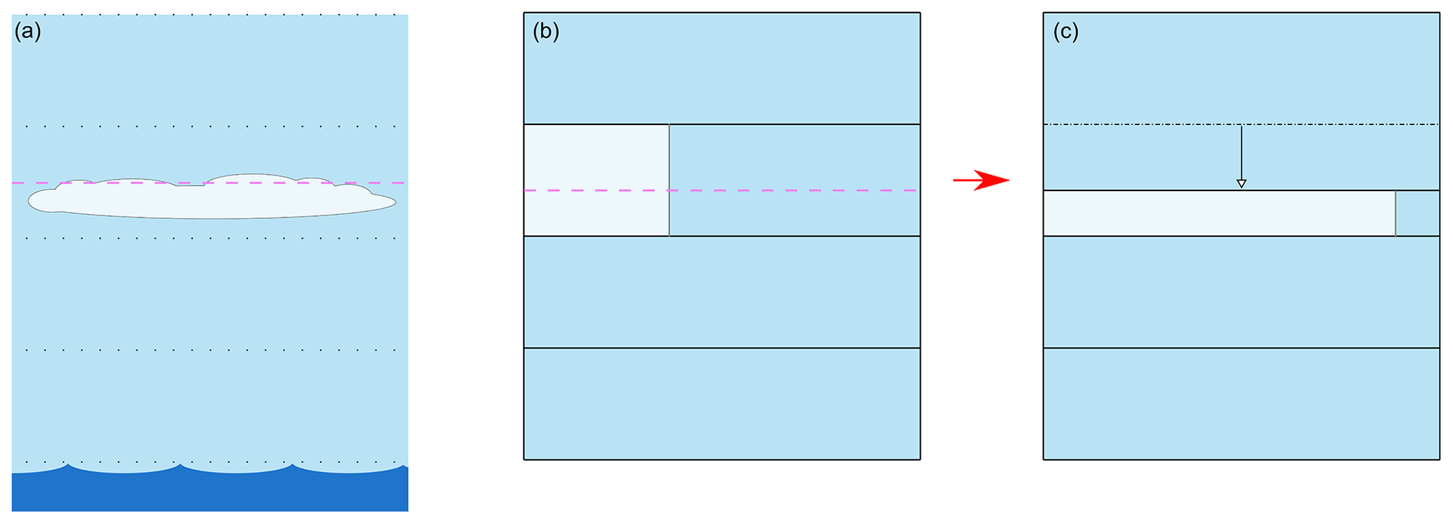
Figure 1 Schematic illustrating the idea behind the new stratocumulus representation method. The pink dashed line represents the temperature inversion. Panel (a) is a depiction of the real situation, panel (b) is its representation in the model's vertical grid, and panel (c) is the same situation on the proposed new vertical grid.

An outline of the method is as follows. First, model columns in which a stratocumulus cloud may be present are identified, and the grid box layer within which the inversion would be found, named the “ambiguous layer”, is selected. The exact location (pressure level) of the inversion is diagnosed using the “reconstructed inversion” method described by Grenier and Bretherton (2001), which assumes a certain sub-grid shape of the temperature profile. The inversion is modelled as a discontinuity in the profile, so that it has a single exact pressure value, usable as the cloud top. Once the inversion pressure is known, the overlying model half-level (representing the cloud top) is shifted down to it, resulting in a thinner lower layer in which the stratocumulus cloud is contained as well a larger but cloud-free above-cloud layer of free-tropospheric air. The values of the relevant physical quantities are finally recalculated on this new grid. The new grid boundaries and recalculated quantities are passed to the radiation routine, and the procedure is repeated at every radiation time step.

With this scheme, the liquid water path (LWP) of the grid layer is conserved: the layer thickness is reduced and the liquid water mixing ratio is proportionally increased. The in-cloud LWP, which is what is used for cloudy-sky radiative calculations, shows a reduction that is inversely proportional to the increase in the cloud fraction. As the radiative flux calculation is linear in the cloud fraction but non-linear in the LWP (and hence in cloud optical depth), there can be a difference in radiative fluxes when applying the invgrid scheme. We present a demonstration of its effect in Appendix A.

The following sections describe the steps in detail, from the detection of applicable columns to the recalculation of all new-grid quantities. The method to calculate the inversion pressure, described in Sect. 2.2.2, closely follows the reconstructed inversion method developed and described by Grenier and Bretherton (2001). The code to calculate the inversion pressure following this procedure was written by Siegenthaler-Le Drian (2010) for her PhD thesis; hence, it is already available in ECHAM-HAM. A few changes implemented during this study are described.

2.2.1 Ambiguous layer selection

The criterion used to select columns in which to apply invgrid at each time step is based on low tropospheric stability (LTS). LTS is a measure defined as the difference in potential temperature between the 700 hPa level and the surface. A strong correlation between LTS and low stratiform cloud cover has been found in observations, especially in the subtropics, as shown by studies such as Klein and Hartmann (1993) and Wood and Hartmann (2006). A high LTS is attributable to a strong inversion. Based on the climatology of low stratus cover in Klein and Hartmann (1993), a threshold LTS value of 20 K is used to select the columns with possible stratocumulus clouds in which to subsequently apply the invgrid scheme. This criterion was previously used by Siegenthaler-Le Drian (2010) to select columns in which to activate her stratocumulus-entrainment parameterisation. As a possible alternative, the threshold could also be based on the estimated inversion strength (EIS), which, as a more refined measure of inversion strength compared with LTS, may be more robust as a predictor of low stratocumulus cloud cover. This is also because, as pointed out by Wood and Bretherton (2006), the relationship between LTS and cloud fraction is not proven to hold in a warming climate, whereas the link between EIS and stratocumulus cloud cover is more direct. In the context of this study, the choice of criterion between LTS or EIS is not expected to produce significant differences in the selection of stratocumulus columns; hence, the simpler option is used.

In each identified column, the layer in which the inversion will be pursued and reconstructed must be selected. This layer is called the ambiguous layer by Grenier and Bretherton (2001) due to the fact that it would exhibit a lower cloudy part of boundary layer air and an upper cloud-free part of free-tropospheric air in reality, but this vertical distinction cannot be resolved within one model grid box. Finding the inversion pressure allows one to separate the two parts. To select the ambiguous layer, we first look for the inversion in the model (i.e. the maximum gradient of temperature). This will be found across two grid layers, which may both potentially contain the inversion jump in a sub-grid profile reconstruction. Between these two layers, we select the uppermost one containing a cloud as the ambiguous layer. The expression “containing a cloud” is defined as “having non-zero cloud cover and liquid water content” (as in the absence of either of these, a cloudy radiative flux is not computed in the model). This selection criterion finds the top of the simulated cloud and, therefore, guarantees that the cloud-rescaling idea would be applicable. If no cloud is present in either of the two possible layers, we use the condition previously used by Siegenthaler-Le Drian (2010): we look at the saturation of an air parcel in an adiabatic ascent from two layers below the inversion, and we choose the ambiguous layer as the layer under the first half-level at which the parcel reaches supersaturation, as it presents the conditions to contain a cloud. This condition operates under the assumption that the stratocumulus is contained within only one layer, as the cloud top could still be found in the layer above. The scheme allows the possibility to reattempt the inversion reconstruction calculation one layer above if it fails in the first selected ambiguous layer.

2.2.2 Inversion reconstruction

We diagnose the inversion pressure following the method developed and described by Grenier and Bretherton (2001); the procedure is repeated here for the convenience of the reader and to indicate our modifications.

The inversion pressure reconstruction method by Grenier and Bretherton (2001) is based on reconstructing the sub-grid profile of virtual liquid water potential temperature (θ_vl) in the ambiguous layer k, in which its value ${\mathit{\theta }}_{\text{vl}}^k$ is considered the weighted average of its below-inversion (boundary layer) and above-inversion (free-tropospheric) values. Figure 2 shows a diagram of an example profile, with labelled layer indices.

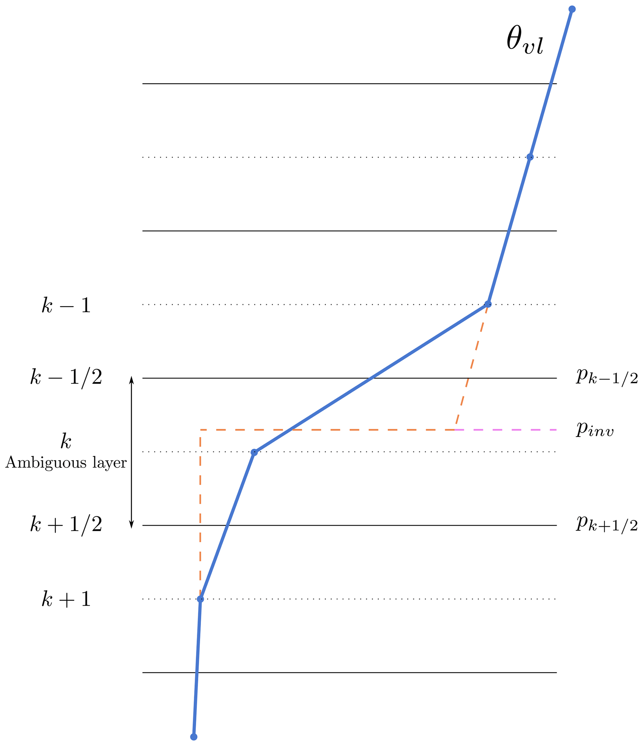
Figure 2 Illustration of a θ_vl profile (blue line) and its sub-grid reconstruction (dashed orange line) in the ambiguous layer. The solid and dotted horizontal black lines are the model half-levels and full-levels respectively. The dashed lines extending from levels k+1 and k−1 represent the assumed sub-grid θ_vl profile within the ambiguous layer and are obtained as described in Sect. 2.2.2. The discontinuity in the sub-grid profile constitutes the inversion pressure p_inv.

The virtual liquid water potential temperature is defined as

$$\begin{array}{}\text{(2)}& {\displaystyle }{\displaystyle }{\mathit{\theta }}_{\text{vl}}=T{\left({\displaystyle \frac{p_{\mathrm{0}}}{p}}\right)}^{\frac{R_{\mathrm{d}}}{c_{\text{pd}}}}\left(\mathrm{1}-{\displaystyle \frac{L_{\mathrm{v}}}{c_{\text{pd}}T}}{r}_{\mathrm{l}}\right)\left(\mathrm{1}+\left({\displaystyle \frac{R_{\mathrm{v}}}{R_{\mathrm{d}}}}-\mathrm{1}\right)r_{\mathrm{t}}\right),\end{array}$$

where T is temperature, p is pressure (p₀=1000 hPa), R_d and R_v are the respective dry air and water vapour gas constants, L_v is the latent heat of vaporisation, r_l and r_t are the respective liquid and total water contents (mass mixing ratios), and c_pd is the constant pressure heat capacity of air. θ_vl depends linearly on temperature and, hence, exhibits the same vertical profile features (notably the inversion), with the advantage of being a conserved quantity in a reversible moist adiabatic process (i.e. a process where all the condensate remains within the air parcel. The inclusion of the “potential” and “liquid water” parts (second and third factors on the right-hand side of the equation) causes the quantity to be conserved, while the “virtual” part (fourth factor) allows one to use the dry-air equation of state. This makes the quantity advantageous to use in calculations; hence, θ_vl is used for the profile reconstruction.

On a sub-grid scale, within the ambiguous layer, we distinguish between an above-inversion and a below-inversion profile, and we assume that θ_vl follows

$$\begin{array}{}\text{(3)}& {\displaystyle }\begin{array}{rl}& {\mathit{\theta }}_{\text{vl}}\left(p\right)=\\ & \left\{\begin{array}{ll}{\mathit{\theta }}_{\text{vl}}^{k+\mathrm{1}},& p_{k+\mathrm{1}/\mathrm{2}}>p>p_{\text{inv}}\\ {\mathit{\theta }}_{\text{vl}}^{k-\mathrm{1}/\mathrm{2}}+s\left(p-p_{k-\mathrm{1}/\mathrm{2}}\right),& p_{\text{inv}}>p>p_{k-\mathrm{1}/\mathrm{2}}\end{array}\right..\end{array}\end{array}$$

Below the inversion, θ_vl has the same value that it does lower down in level k+1; this is justified by the fact that the boundary layer tends to be very well mixed in the case of a strong inversion, in which case θ_vl is constant throughout the well-mixed layer. Above the inversion, the θ_vl profile is extrapolated down from the overlying level, using the maximum negative gradient with respect to pressure (s) chosen from the gradients across half-levels $k-\mathrm{1}/\mathrm{2}$ or $k-\mathrm{3}/\mathrm{2}$.

This profile implies that at the inversion pressure p_inv, θ_vl experiences a discontinuity, where the value jumps from the boundary layer to the free troposphere, representing the sharp inversion. The inversion pressure is found by requiring conservation of θ_vl within the ambiguous layer, i.e. by requiring that the integral of the sub-grid profile is equal to the original value of θ_vl in the ambiguous layer k (${\mathit{\theta }}_{\text{vl}}^k$, considered to be the grid box average):

$$\begin{array}{ll}\text{(4)}& {\displaystyle }{\mathit{\theta }}_{\text{vl}}^k& {\displaystyle }={\displaystyle \frac{\mathrm{1}}{p_{k+\mathrm{1}/\mathrm{2}}-p_{k-\mathrm{1}/\mathrm{2}}}}\underset{p_{k-\mathrm{1}/\mathrm{2}}}{\overset{p_{k+\mathrm{1}/\mathrm{2}}}{\int }}{\mathit{\theta }}_{\text{vl}}\left(p\right)\mathrm{d}p{\displaystyle }& {\displaystyle }={\displaystyle \frac{\mathrm{1}}{p_{k+\mathrm{1}/\mathrm{2}}-p_{k-\mathrm{1}/\mathrm{2}}}}\left(\underset{p_{k-\mathrm{1}/\mathrm{2}}}{\overset{p_{\text{inv}}}{\int }}{\mathit{\theta }}_{\text{vl}}^{k-\mathrm{1}/\mathrm{2}}+s\left(p-p_{k-\mathrm{1}/\mathrm{2}}\right)\mathrm{d}p\right.\\ \text{(5)}& {\displaystyle }& {\displaystyle }\left.+\underset{p_{\text{inv}}}{\overset{p_{k+\mathrm{1}/\mathrm{2}}}{\int }}{\mathit{\theta }}_{\text{vl}}^{k+\mathrm{1}}\mathrm{d}p\right).\end{array}$$

In order to solve Eq. (5) for the inversion pressure, we define the above-inversion mass fraction of the ambiguous layer as follows:

$$\begin{array}{}\text{(6)}& {\displaystyle }{\displaystyle }\mathit{\mu }={\displaystyle \frac{p_{\text{inv}}-p_{k-\mathrm{1}/\mathrm{2}}}{p_{k+\mathrm{1}/\mathrm{2}}-p_{k-\mathrm{1}/\mathrm{2}}}}.\end{array}$$

Equation (5) can then be turned into a quadratic equation in μ:

$$\begin{array}{ll}{\displaystyle }& {\displaystyle \frac{\mathrm{1}}{\mathrm{2}}}s\left(p_{k-\mathrm{1}/\mathrm{2}}-p_{k+\mathrm{1}/\mathrm{2}}\right){\mathit{\mu }}^{\mathrm{2}}-\left({\mathit{\theta }}_{\text{vl}}^{k-\mathrm{1}/\mathrm{2}}-{\mathit{\theta }}_{\text{vl}}^{k+\mathrm{1}}\right)\mathit{\mu }\\ \text{(7)}& {\displaystyle }& {\displaystyle }+\left({\mathit{\theta }}_{\text{vl}}^k-{\mathit{\theta }}_{\text{vl}}^{k+\mathrm{1}}\right)=\mathrm{0}.\end{array}$$

The physical solution for μ is a value between zero and one which, when it exists, can be shown to be the smaller solution of Eq. (7). If and when a physical μ is found, the inversion pressure p_inv is obtained inversely from Eq. (6). In a following step, p_inv is used to define the new grid.

A limitation of this method is that it requires a well-mixed θ_vl profile in the PBL to successfully obtain the inversion pressure; specifically, the θ_vl gradient with respect to pressure must be negative both below and above the inversion. While this is a characteristic of stable profiles, we noticed that the method sometimes gave inconsistent results when the profiles slightly deviated from being well mixed. We included a few minor modifications to the method to allow it to be used in more, although less ideal, situations. For example, we force a small but negative s ($-\mathrm{1}\times {\mathrm{10}}^{-\mathrm{6}}$ K Pa⁻¹) if the gradient above the inversion is only slightly positive (which would normally be considered unusable). We also attempt to carry out the inversion reconstruction in the upper possible ambiguous layer if it fails in the lower one.

2.2.3 Grid refinement

As the new representation is used exclusively in the radiation routine, the grid refinement is applied only in cases where it would make a difference to the radiative transfer calculations, specifically by increasing the cloud cover. Hence, we first check that the ambiguous layer contains a cloud, as this is a necessary condition for the radiation routine to compute a cloudy flux. We also ensure that the grid box layer would not become thinner than a minimum thickness. The limit is put in place to prevent unphysical situations, such as an overly high liquid water mixing ratio or cloud droplet concentration. We choose a threshold of 50 m, as stratocumuli are almost never observed to be thinner (cf. the histogram of observed instantaneous cloud thicknesses in Wood, 2012).

If the conditions are appropriate, we proceed with defining the new refined grid. The half-level above the inversion, the top of the ambiguous layer, is shifted down to the inversion pressure p_inv. Level k becomes thinner and will wholly contain the cloud that was originally present in the ambiguous layer. In the case of multilevel clouds, the lower layers are unaffected. Level k−1, on the other hand, becomes larger and will represent the first layer of free-tropospheric air.

Once the new grid is defined, the variables that need to be passed to the radiation routine are calculated in the new layers using the assumed sub-grid profile, conservation principles, and the notion that the stratocumulus cloud in the new grid is constrained below the inversion. The procedure for each variable is detailed in the following. Superscripts k and k−1 refer to variables and layers in the original model grid, i.e. the ambiguous layer and the overlying layer respectively. We use superscript kinv for the new thinner layer (equivalent to the below-inversion fraction of the ambiguous layer), superscript abinv for the above-inversion fraction of the ambiguous layer (note that this is not a layer in its own right on either grid), and superscript kinv−1 for the new larger overlying layer, consisting of layers abinv and k−1.

Water content reconstruction

The water vapour, liquid water, and ice contents are defined as mass mixing ratios ($\mathrm{kg}{\mathrm{kg}}_{\mathrm{air}}^{-\mathrm{1}}$) in the model (r_v, r_l and r_i respectively). The total water mixing ratio r_t is the sum of all three individual phases and must be conserved across the affected layers.

For consistency with θ_vl, we require that r_t follows the same sub-grid profile in the ambiguous layer, and we start by calculating it as follows:

$$\begin{array}{}\text{(8)}& {\displaystyle }& {\displaystyle }{r}_{\mathrm{t}}^{\text{kinv}}=r_{\mathrm{t}}^{k+\mathrm{1}}\text{(9)}& {\displaystyle }& {\displaystyle }{r}_{\mathrm{t}}^{\text{abinv}}={\displaystyle \frac{r_{\mathrm{t}}^k-(\mathrm{1}-\mathit{\mu })r_{\mathrm{t}}^{k+\mathrm{1}}}{\mathit{\mu }}},\end{array}$$

where the second equation is a solution to conservation of r_t in layer k, given the above-inversion mass fraction μ of the ambiguous layer. Its value in kinv−1 is obtained as a mass-weighted average of abinv and k−1:

$$\begin{array}{}\text{(10)}& {\displaystyle }{\displaystyle }{r}_{\mathrm{t}}^{\text{kinv}-\mathrm{1}}={\displaystyle \frac{r_{\mathrm{t}}^{\text{abinv}}{M}^{\text{abinv}}+r_{\mathrm{t}}^{k-\mathrm{1}}{M}^{k-\mathrm{1}}}{M^{\text{abinv}}+M^{k-\mathrm{1}}}},\end{array}$$

where M is the air mass of a layer, and the denominator is equal to the air mass in kinv−1.

As liquid water and ice are the components that make up the cloud, we restrict them to be found only below the inversion, in the new thinner cloud layer kinv. The total liquid and ice mass is conserved, which means that the mixing ratio is simply rescaled to the new layer mass:

$$\begin{array}{}\text{(11)}& {\displaystyle }{\displaystyle }{r}_{\mathrm{l}/\mathrm{i}}^{\text{kinv}}=r_{\mathrm{l}/\mathrm{i}}^k{\displaystyle \frac{M^k}{M^{\text{kinv}}}}.\end{array}$$

Thus, the quantities r_l and r_i are assumed to be zero in abinv, and the values in k−1 are rescaled to the larger layer for layer kinv−1. This recalculation does not change the total in-cloud amounts of liquid and ice water, as the cloud volume is conserved.

The calculation of the water vapour mixing ratio in the new layers kinv and kinv−1 uses the previously calculated reconstructed total water and the inversion-constrained liquid and ice water mixing ratios:

$$\begin{array}{}\text{(12)}& {\displaystyle }{\displaystyle }{r}_{\mathrm{v}}=r_{\mathrm{t}}-r_{\mathrm{l}}-r_{\mathrm{i}}.\end{array}$$

We recognise that the method for recalculating the water contents described in this section is not fully consistent. In fact, the total water content is treated as a separate variable (as opposed to using the sum of the individual phases of water) and is reconstructed using the sub-grid profile which depends on the under- and overlying layers; at the same time, the liquid and ice contents are taken from the ambiguous layer and simply moved to the below-inversion part. This can lead to an inconsistency in the water vapour content – especially in the new cloudy layer kinv (in which the air should be saturated), as it is calculated by subtracting the rescaled liquid and ice contents (from layer k) from the total r_t (from layer k+1). In kinv−1, the inconsistency is negligible, as there should be no liquid or ice water there. We decided to move forward with this method despite this problem because it has the following advantages: (1) the liquid and ice contents used for the cloud are the ones that are calculated in the cloud microphysics routine, which takes fundamental microphysical processes into account; (2) the resulting total water below the inversion is equal to that in the layer below, as is characteristic of well-mixed boundary layers. Overall, the method gives reasonable results for r_v above the inversion and for r_l and r_i in the cloudy layer below it, and the total water content, as the sum of the individual components, is indeed conserved. Checks are in place to prevent and fix potential unphysical (negative) values of r_v, r_l, r_i, or r_t.

Temperature

The temperature on the new grid is calculated using energy conservation. First, in kinv, T is obtained inversely from ${\mathit{\theta }}_{\text{vl}}^{\text{kinv}}$ (Eq. 2). The internal energy U of the original layers k and k−1 is then calculated, along with the internal energy of new layer kinv:

$$\begin{array}{}\text{(13)}& {\displaystyle }{\displaystyle }{U}^j=\left(c_{\text{pd}}+c_{\text{pv}}{r}_{\mathrm{v}}^j+c_{\text{lw}}{r}_{\mathrm{l}}^j+c_{\text{iw}}{r}_{\mathrm{i}}^j\right)M^j{T}^j,\end{array}$$

where superscript j indicates the layer considered, and c_pv, c_lw and c_iw are the respective vapour, liquid water, and ice specific heat capacities. Then, for energy conservation over the two layers between the original and new grid, T^kinv−1 is obtained from

$$\begin{array}{ll}{\displaystyle }& {\displaystyle }{T}^{\text{kinv}-\mathrm{1}}=\\ \text{(14)}& {\displaystyle }& {\displaystyle \frac{U^k+U^{k-\mathrm{1}}-U^{\text{kinv}}}{\left(c_{\text{pd}}+c_{\text{pv}}{r}_{\mathrm{v}}^{\text{kinv}-\mathrm{1}}+c_{\text{lw}}{r}_{\mathrm{l}}^{\text{kinv}-\mathrm{1}}+c_{\text{iw}}{r}_{\mathrm{i}}^{\text{kinv}-\mathrm{1}}\right)M^{\text{kinv}-\mathrm{1}}}}.\end{array}$$

Further cloud variables

Similar to r_l and r_i, we confine all cloud variables of the ambiguous layer k to the new thinner layer kinv, which is capped by the inversion. The recalculation invokes conservation of cloud volume for cloud cover (clc), and particle number for cloud droplet and ice crystal number concentrations (n_cd, n_ic). The variables are simply scaled to the new layer thickness Z and essentially “squeezed” under the inversion:

$$\begin{array}{}\text{(15)}& {\displaystyle }& {\displaystyle }{n}_{\text{cd/ic}}^{\text{kinv}}=n_{\text{cd/ic}}^k{\displaystyle \frac{Z^k}{Z^{\text{kinv}}}},\text{(16)}& {\displaystyle }& {\displaystyle }{\text{clc}}^{\text{kinv}}={\text{clc}}^k{\displaystyle \frac{Z^k}{Z^{\text{kinv}}}}.\end{array}$$

The cloud cover is of course constrained so as not to exceed 100 %.

The new half- and full-level pressures (grid boundaries) and all of the recalculated new-grid variables are finally passed to the radiation routine.

Note that the aerosol tracers are not regridded in invgrid. The slight alteration of the invgrid radiative effect due to this is of secondary importance to the effects caused by changes in cloud cover and condensate. The more important aerosol effects on clouds and how they are parameterised are kept the same.

2.3 Model versions

The model versions that were used to perform the simulations discussed in the next sections are presented in the following. In addition to the reference model version (REF), two versions implementing invgrid were used: one that rescales cloud cover based on cloud volume conservation, as described above, (SC-VOLUME), and one that recalculates the cloud cover on the refined grid by rerunning the model's Sundqvist cloud cover scheme (SC-SUND). Another simple scheme (SC-MAX) was used to test and provide an understanding of the potential and limitations of the different invgrid versions.

2.3.1 REF

The model version ECHAM(v6.3)-HAM(v2.3)-P3 is used as the base model version and is referred to as REF (Dietlicher et al., 2018; Tegen et al., 2019). Simulations conducted with REF illustrate the baseline performance of the model and provide the reference to which simulations conducted with the new schemes developed in this thesis are compared. A brief description of REF and its relevant schemes is given in Sect. 2.1 of this paper.

2.3.2 SC-VOLUME

In the SC-VOLUME model version, the invgrid scheme described in Sect. 2.2 is fully implemented in the model. The calculation of the inversion pressure (as in Sect. 2.2.2) is performed at every time step before the radiation routine for diagnostic reasons. At radiation time steps, the value is used to refine the vertical grid; physical variables are recalculated as described in Sect. 2.2.3, with the stratocumulus cloud cover calculation being based on cloud volume conservation. These are passed to the radiation routine.

2.3.3 SC-SUND

In the SC-SUND model version, after executing the invgrid grid refinement, the stratocumulus cloud cover is calculated by running the model's Sundqvist cloud cover scheme. This is done regardless of the original cloud cover. The specific goal here is to address cases in which, on the original grid, no cloud is present in the ambiguous layer. This could be due to the ambiguous layer's water vapour mixing ratio being an average between dry tropospheric air and moist boundary layer air, which may cause the grid box average relative humidity to be too low to reach the threshold for forming cloud cover according to Eq. (1). With the new grid's reconstruction, the two different air masses are separated, which may allow a cloud to form in the new thinner layer, now made up exclusively of boundary layer air and, hence, presumably having a higher relative humidity. This would be valuable because it would lead to a better representation of stratocumulus clouds in layers in which the SC-VOLUME method could not be applied due to the initial lack of a cloud in the model. This method makes use of the refined grid and recalculated profiles of water content and temperature, but the cloud volume is not necessarily conserved as the cloud cover is recomputed with the cloud cover scheme. The procedure is only applied if the layer in which a new cloud cover is calculated already contains liquid water (or cloud ice), to ensure the presence of a “real” cloud (having cloud cover and water condensate), as the Sundqvist cloud cover scheme itself does not consider or affect the presence of condensate. The new cloud cover representation is only used in the radiation routine.

2.3.4 SC-MAX

The SC-MAX model version was designed to investigate the maximum possible effect of a scheme that increases the cloud cover of existing stratocumuli, such as in SC-VOLUME. This is done by always increasing the cloud cover to 100 % in model layers where a stratocumulus cloud is identified. The cloud cover increase is applied in the same cases in which SC-VOLUME's cloud rescaling would be (i.e. when the identified ambiguous layer contains a cloud) but also when the ambiguous layer contains no cloud but another layer (at most two levels below it) does. We still consider the latter case as a stratocumulus cloud. The cloud cover of the first (uppermost) cloudy model layer below the inversion is set to 100 %. The modified cloud cover is passed to the radiation routine.

2.4 Experiment description

For each model version, we performed a 15-year-long (2000–2014) global climate simulation with prescribed sea-surface temperatures (PCMDI, 2018) from the Atmospheric Model Intercomparison Project (AMIP) to evaluate the stratocumulus cloud representation. We used the standard ECHAM-HAM T63/L47 spatial resolution and 450 s (7.5 min) time step. The data from the invgrid routine are sampled at radiation time steps (i.e. every 2 h). As an observational reference for total cloud cover, we used Cloud-Aerosol Lidar and Infrared Pathfinder Satellite Observations (CALIPSO) data from the GCM-Oriented CALIPSO Cloud Product (GOCCP) dataset (Chepfer et al., 2010; Bony and Chepfer, 2013).

3 Results and discussion

3.1 Single-column model

We first tested invgrid's inversion reconstruction and grid refinement in ECHAM-HAM's single-column model (SCM) mode (Dietlicher et al., 2018). Using the SCM allows us to closely observe the evolution of the vertical profiles and how invgrid responds to them. Additionally, the possibility to use observational forcings for the SCM is a method to test the model's representation of real situations and to generally validate the reconstructions of the new scheme. The validation in the SCM was carried out using a forcing derived from observations made during the East Pacific Investigation of Climate (EPIC) campaign (Bretherton et al., 2004), specifically from a segment between 16 and 22 October 2001 in the southeastern Pacific, where the vertical structure of the boundary layer capped by a persistent stratocumulus cloud was observed using radiosondes and remote sensing (Bretherton, 2005). The EPIC campaign also provided observations of the cloud top and base in this period, obtained with cloud radar and ceilometer respectively (Caldwell et al., 2005), which are used to validate the inversion heights found.

Figure 3 shows the evolution of the cloud top and base over the 6 d period of the EPIC campaign. The cloud top follows the PBL's diurnal cycle, rising during the night due to long-wave cloud top cooling driving entrainment and sinking during the day due to the absorption of solar radiation suppressing entrainment. The reconstructed inversion generally captures this diurnal cycle. While the exact height of the inversion is at times overestimated (days 1, 4), most of the time it matches the observed cloud top quite well, especially on days 2, 3, and 6. The occasional sudden jumps in the inversion pressure (e.g. between days 1 and 2) occur due to the selection criterion for the ambiguous layer depending on the maximum gradient of θ_vl, whose level can change suddenly when the inversion is not very sharp. Finding a criterion which could address this undesirable issue without loss of generality proved difficult. We also calculated the lifting condensation level (LCL) for an air parcel rising from the surface to attempt to estimate the cloud base, but the results exhibited large oscillations and did not match the cloud base most of the time, rendering the LCL diagnostic unsuitable as a proxy for cloud base. A reconstruction of the cloud base would be beneficial to the scheme to complement the constraint of the cloud's extent from above with a constraint from below, resulting in a further improved representation, but the development of a method for accurately diagnosing the cloud base of stratocumulus clouds is outside the scope of this study. In comparison to the inversion reconstruction performed by Siegenthaler-Le Drian (2010), who also tested it in the SCM with the EPIC data, with the modifications added in our method, the inversion is also found in cases where the method previously failed – for example, at the start of the day 1 or during day 6.

Figure 3 Observed cloud base and top during the stratocumulus segment of the EPIC campaign (Bretherton, 2005), and reconstructed inversion and lifting condensation level height. The grey dashed horizontal lines are model half-levels in ECHAM-HAM. The time series starts on 15 October 2001 at 18:00 LT. The cloud and its boundaries as represented by the model can be seen in Fig. 5 (REF).

For further validation, we also ran the EPIC SCM experiment with different relaxation timescales and perturbed initial conditions; the results are presented in Appendix B. Overall, the inversion reconstruction method gives good results with respect to finding the location of the stratocumulus cloud top.

We show some example vertical profiles that occurred during EPIC to illustrate the effect of the grid refinement on temperature, total water mixing ratio, and cloud cover in Fig. 4. The inversion in the physical quantities is sharper and demonstrates the better separation between the PBL and the free troposphere on the refined grid. The cloud cover increases by 6 percentage points – or by almost 30 % – as a result of the lower vertical extent of the layer.

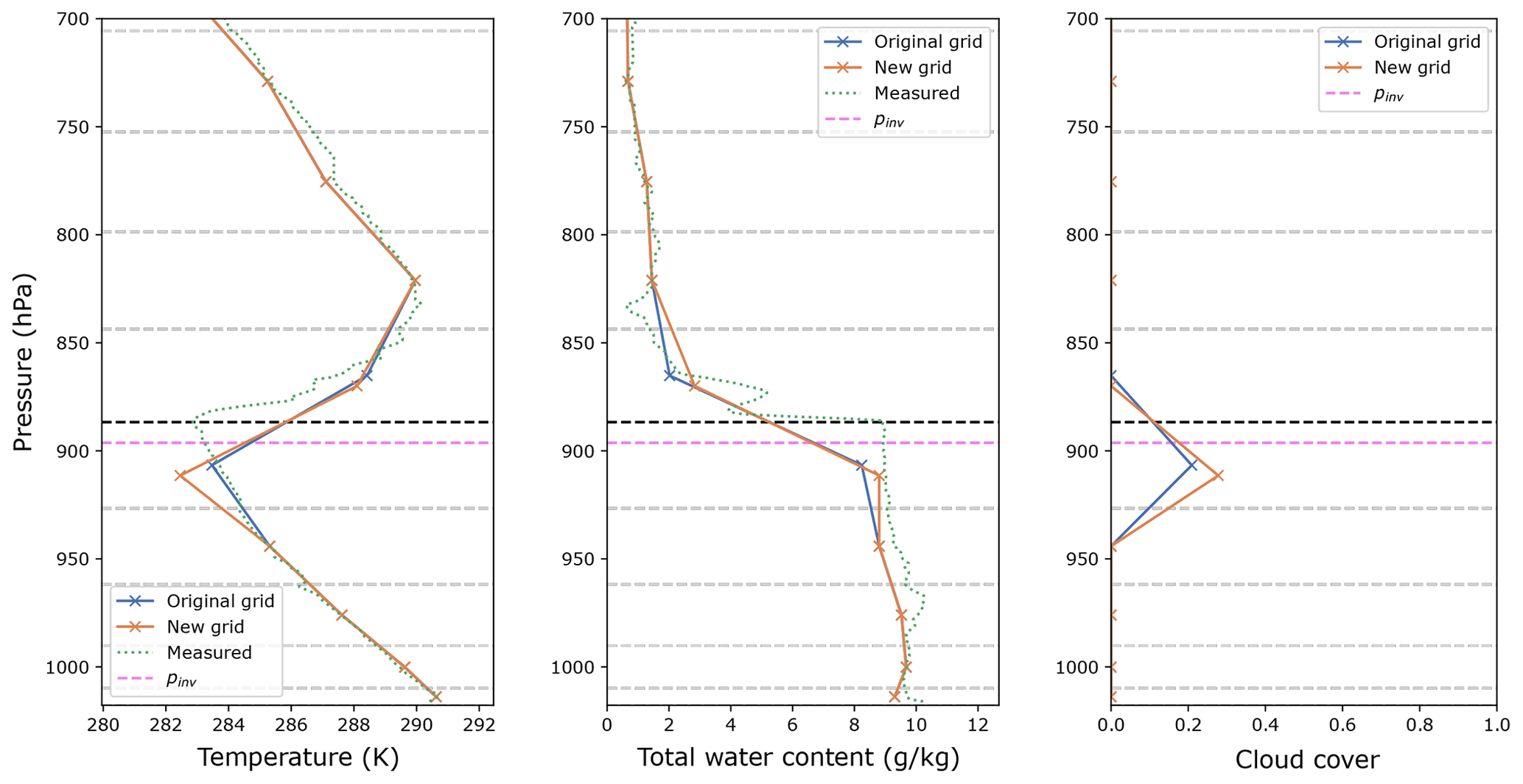
Figure 4 Example vertical profiles of the EPIC SCM experiment obtained with the original and new (refined) model grid and observed profiles at the end of day 5 (hour 118). The grey dashed lines represent half-levels common to both grids. The black dashed line represents the top of the ambiguous layer on the original grid; it is shifted to the inversion pressure (magenta dashed line) for the refined grid.

Table 1 Annual mean total cloud cover and differences between simulations, as global and regional averages. An asterisk denotes statistically significant differences at the 95 % significance level. “Δ seen by rad.” indicates the change in total cloud cover produced with invgrid, which is then applied only in the radiation routine. The abbreviations used in this table (and in subsequent tables throughout the paper) are as follows: North America (NAM), South America (SAM), southern Africa (AFR), and the Barents Sea (BAR).

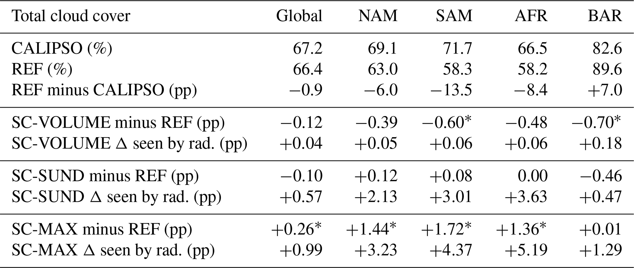
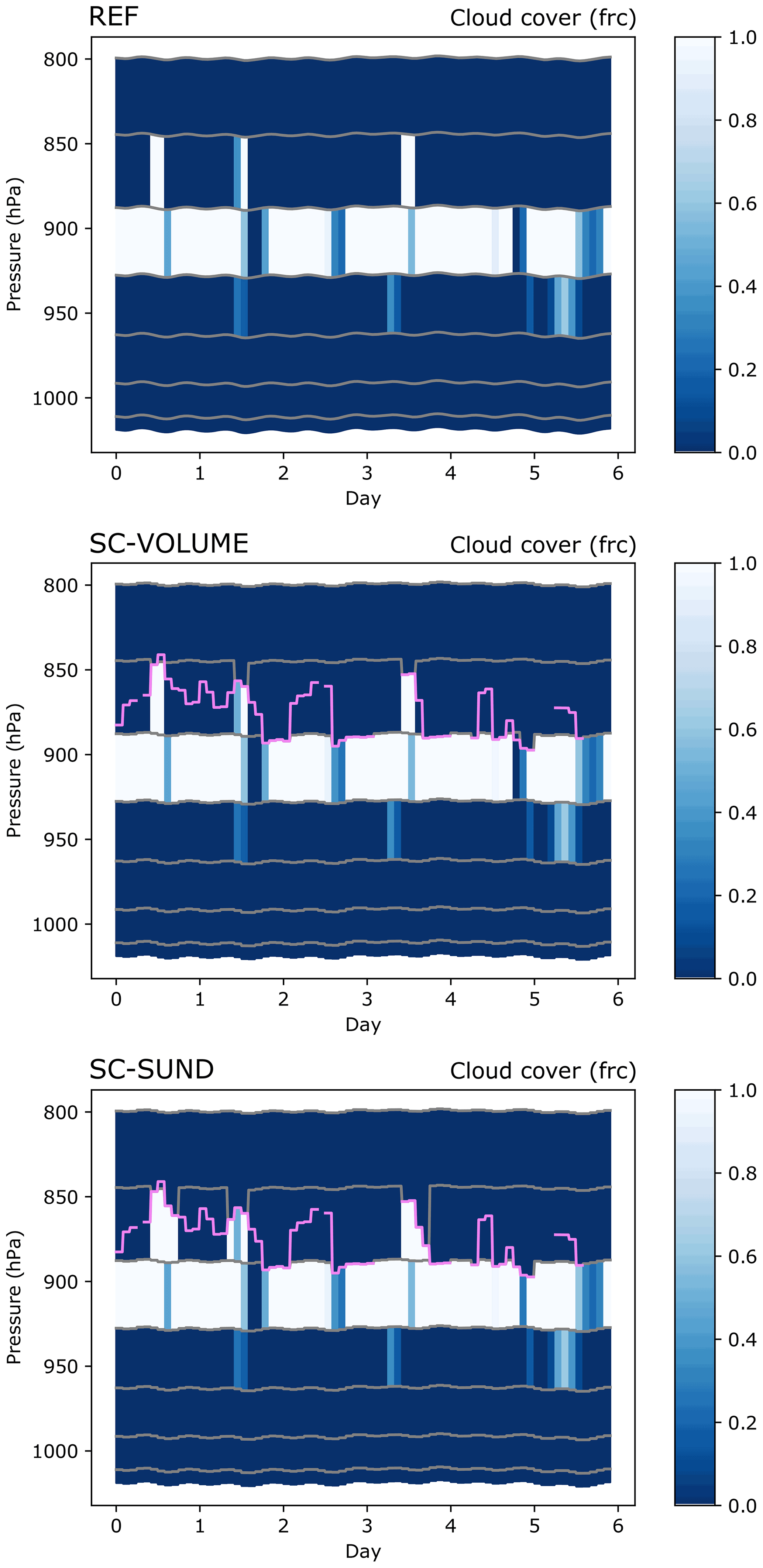
Figure 5 Cloud cover fraction of clouds in the EPIC SCM simulations in REF, SC-VOLUME, and SC-SUND. The grey lines represent the model half-levels, and the magenta line is the reconstructed inversion pressure. The inversion's evolution in time appears more steplike than in Fig. 3 because the refined grid is only applied for the radiation routine at radiation time steps (every 7200 s).

The EPIC SCM experiment was simulated with the REF, SC-VOLUME, and SC-SUND model set-ups; Fig. 5 shows the cloud cover below 800 hPa for each experiment. Only the cloud cover belonging to layers that also have a non-zero liquid water content is shown. In the REF simulation, the cloud is mostly contained within one layer in the model. In fact, it is most often found in the layer below the one containing the inversion and, hence, in which the cloud top was predicted (and observed) to reside. In these situations, the cloud rescaling cannot be applied with SC-VOLUME, as the layer containing the inversion contains no cloud; hence, the reconstruction would not make a difference to the radiation routine. The three times that the model's cloud extends into the upper layer, the invgrid scheme is applied effectively, reducing the thickness of the top cloudy layer following the inversion and, hence, obtaining a more realistic depiction. The SC-SUND scheme version was developed in response to the issue described above: it uses a better water profile representation by also applying the refined grid in the cloud cover routine, so that a new cloud can possibly be formed right below the inversion that is missing when using the original grid. In the SC-SUND simulation, a new cloud is formed in a few cases in the upper layer (days 1, 2, and 4) and once in the central layer at the end of day 5. The scheme actually simulates new cloud cover more frequently, but the lack of water condensate in the inversion layer limits the number of “valid” instances. A more ideal representation of the water content in addition to clc would be obtained if the grid refinement method were also used in the microphysics routines. Such an implementation comes with the aforementioned challenges that our more limited usage of the new scheme, which was restricted to the radiation routine, aimed to avoid.

In our analysis of the global simulations we also investigate the frequency of situations such as those observed in the EPIC simulations, in which the model's simulated cloud is in the layer below where we expect to find it via the inversion reconstruction.

3.2 Global climate simulations

After demonstrating the desired functioning of invgrid in the SCM, we studied its effect on the stratocumulus cloud cover in global climate simulations. We focus on three subtropical stratocumulus regions that are known to exhibit semi-permanent marine stratocumulus sheets, namely the oceans just west of North America (NAM), South America (SAM), and southern Africa (AFR). We also look at an Arctic region, over the Barents Sea (BAR). The regional averages cited in the text are defined over the areas highlighted in Fig. 6a.

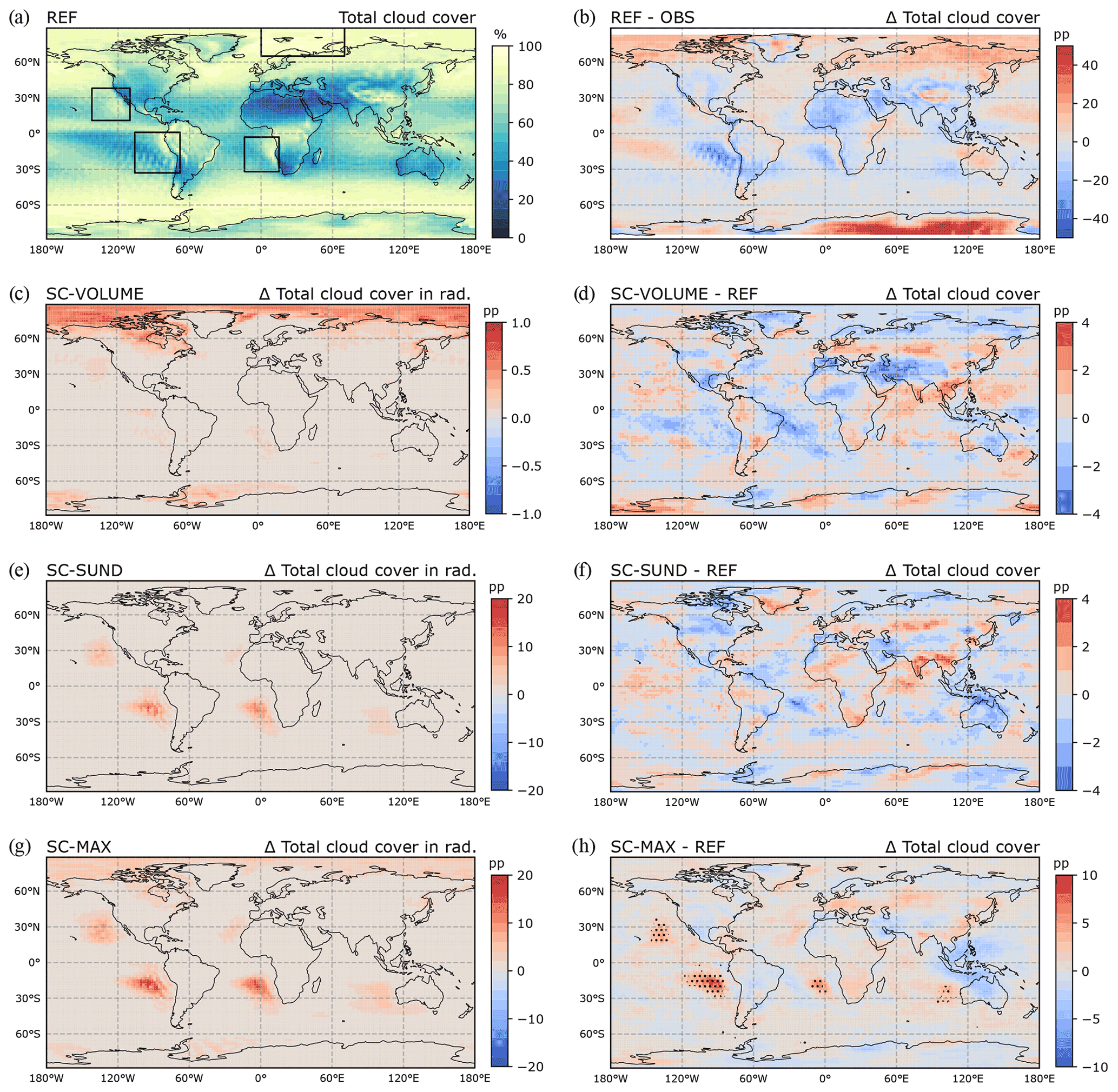
Figure 6 Total cloud cover results from 15-year free global climate simulations. The top row shows the reference results (REF) for (a) total cloud cover and (b) the difference with CALIPSO climatology. The remaining panels (c–h) show the results with SC-VOLUME, SC-SUND, and SC-MAX: the left column displays the total cloud cover increase exerted in the radiation routine, and the right column displays the change in the simulated total cloud cover compared with REF (stippling indicates statistically significant differences at the 95 % significance level; the false discovery rate is controlled following Wilks, 2016). The regions highlighted in panel (a) are defined as follows: NAM (38–11^∘ N, 142–110^∘ W); SAM (1^∘ N–33^∘ S, 106–68^∘ W); AFR (3–32^∘ S, 14^∘ W–15^∘ E); BAR (90–65^∘ N, 0–70^∘ E).

The reference model version REF generally underestimates cloud cover in the subtropical stratocumulus regions, as shown in Fig. 6b in a comparison to the CALIPSO-GOCCP satellite climatology (Chepfer et al., 2010). The cloud cover difference exhibits a similar pattern in all three regions: compared with observations, cloud cover is actually overestimated along the coast, such that the overall underestimation results from large areas of lower cloud cover further offshore. In the Arctic, total cloud cover is instead overestimated by the model.

The results from the simulations with the modified schemes are shown in Fig. 6c–h, with the annual mean simulated total cloud cover on the right-hand side and the total cloud cover change experienced by the radiation routine on the left-hand side (i.e. the difference post- and pre-application of the invgrid scheme). The total cloud cover in the simulations can change when changes from the invgrid scheme to cloud radiative effects feed back on the clouds (e.g. by increased turbulence through stronger cloud top cooling). Regional averages are reported in Table 1.

In the SC-VOLUME simulation, the increase in total cloud cover caused by invgrid and seen by radiation in the annual mean is extremely small in stratocumulus regions, reaching at most 1 percentage point (pp) in the Arctic where it is most marked. As the changes in the radiation routine are small, the change induced in the simulated cloud cover due to internal climate feedback is also very small. A simple two-sided t test using the annual means showed that the results do not differ from REF in a statistically significant manner; they also do not exhibit an explicable pattern (Fig. 6d). The changes in cloud radiative effects produced with SC-VOLUME were much weaker than we had initially expected (not shown), and we investigate the factors that limit the effectiveness of the SC-VOLUME method in global simulations in Sect. 3.3.

In the SC-SUND simulation, the possibility to form new clouds on the refined grid provides the potential to produce a larger mean cloud cover increase than with SC-VOLUME. This is in fact the case in the radiation routine (Fig. 6e): as intended, the subtropical stratocumulus regions exhibit large increases (up to 15 pp) in the annual mean total cloud cover. The most affected areas are located away from the continental coasts (i.e. in the regions where ECHAM-HAM most underestimates cloud cover), showing that SC-SUND can accurately address the problem. As for the change induced in the simulated total cloud cover (Fig. 6f), the difference to REF is also small (of the same order of magnitude as with SC-VOLUME), although the spatial patterns seem to indicate a slight reduction in the model bias in subtropical stratocumulus regions. The stronger cloud top radiative cooling could favour convection bringing moisture into the cloud from the surface, thereby increasing stratocumulus cloud longevity in a positive feedback loop and affecting the simulated cloud cover. However, the difference with REF was also not found to be statistically significant for SC-SUND.

With both set-ups, the change exerted is too small to cause significant changes in the simulated total cloud cover. At the same time, the results indicate that, in terms of the initial changes produced in the radiation routine, SC-SUND is more effective than SC-VOLUME at increasing cloud cover in the annual mean. This suggests that the model's bias is less due to an underestimation of cloud extent in individual instances, which SC-VOLUME is designed to address, and more to a negative bias in the frequency of stratocumulus cloud formation, which can be addressed by SC-SUND due to its re-evaluation of cloud cover on the refined grid. Other factors hindering the suitability of SC-VOLUME could also be at play, and they are considered in the following section.

3.3 Further analysis and scheme limitations

3.3.1 Scheme usage frequency in SC-VOLUME

For SC-VOLUME's cloud cover reconstruction to produce a significant effect in global simulations, it must be applied frequently in practice. The invgrid scheme requires a series of conditions to be met in order to be applied and to rescale the ambiguous layer's cloud cover. The occurrence frequency of these conditions in the SC-VOLUME simulation is reported in Table 2.

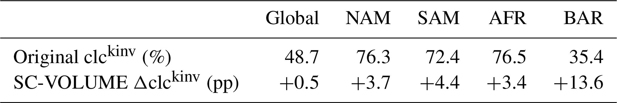
Table 2 Global and regional average occurrence frequency in the SC-VOLUME simulation of finding an inversion, finding an inversion with an underlying cloud (identified stratocumulus clouds), and finding a cloud in the ambiguous layer (AL); and the conditional occurrence frequency of a cloud in the ambiguous layer, given that a cloud is present below the inversion. Also included for comparison are the average frequency of occurrence of stratocumulus clouds from the Hahn and Warren (2007) surface-based observational cloud climatology, averaged over the stratocumulus regions defined in this study.

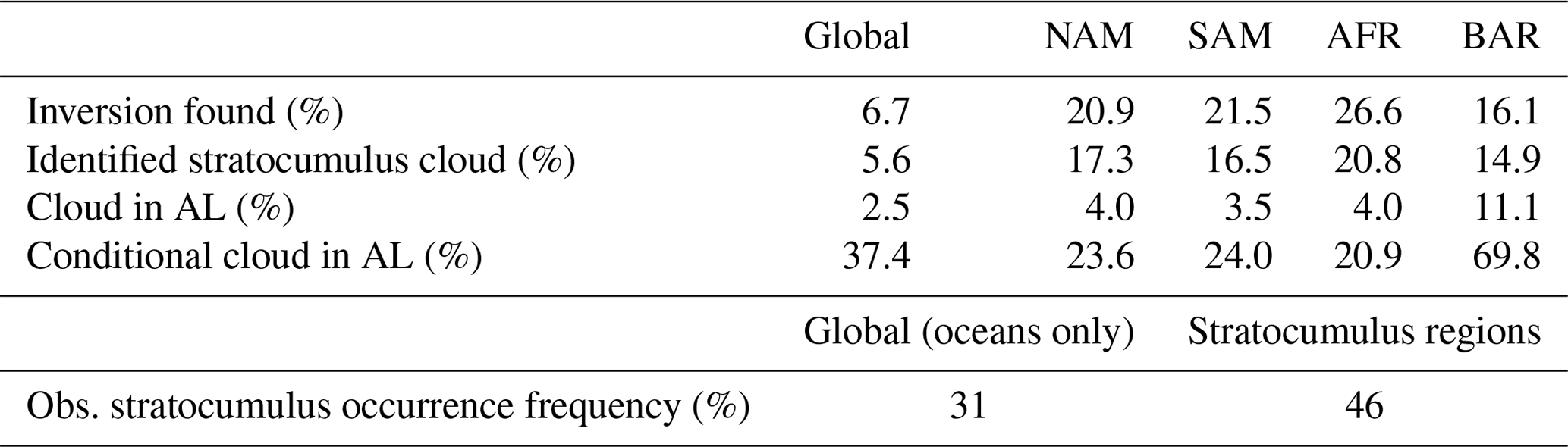
First of all, the scheme must find and successfully reconstruct a temperature inversion. The associated conditions and calculations, described in Sect. 2.2.1 and 2.2.2, result in the inversion being found very frequently in the stratocumulus regions, upwards of 70 % in some columns (Fig. 7a). In most of these cases, a stratocumulus cloud, defined as a cloudy layer at or below the inversion, is also present (Fig. 7b). The occurrence frequency of these identified stratocumulus clouds is lower than in reality, where it is around 46 % annually in the relevant regions according to the ship-based observational climatology (1954–1997) by Hahn and Warren (2007). This represents a deficiency of the model and a limitation to the SC-VOLUME scheme's aptness to correct the cloud cover bias. The method can only target errors in cloud cover amount when a cloud is present, so a model bias in cloud occurrence frequency puts an a priori limit on its possible benefit. The practical applicability of SC-VOLUME's cloud reconstruction method is even more starkly reduced by the subsequent necessary condition that the cloud (or at least its upper part) must be found in the same model layer as the inversion. As indicated in Sect. 3.1 and quantified in Fig. 7c, this condition is in fact very rare and occurs in much more limited areas than those in which stratocumulus clouds are identified, concentrated in close proximity of the coasts. Figure 7d shows the conditional probability of the stratocumulus cloud being found in the ambiguous layer, given that a cloud is present below the inversion. This probability decreases with the distance from the coast in the subtropical marine stratocumulus regions, where it is less than 25 % overall. The rest of the time, the cloud is at a lower level than the inversion. The conditional probability is instead very high at higher latitudes. This is likely the result of the different meteorological conditions – due to lower temperatures and the presence of ice, the model's RH requirement for cloud cover formation is lower and easier to reach. In addition, the PBL is typically shallower in the Arctic, and as the model's vertical resolution is higher closer to the surface, its vertical structure is better resolved and can more easily form clouds at the right level.

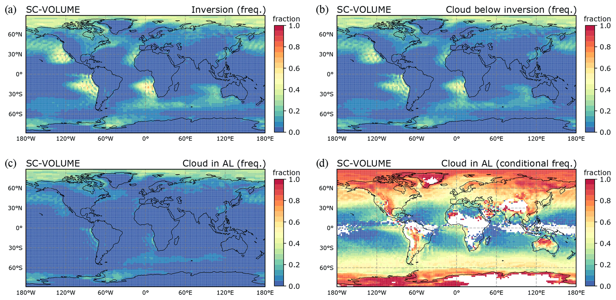
Figure 7 Frequency of occurrence of various conditions related to invgrid in the SC-VOLUME simulation: (a) an inversion is found; (b) a cloud is present below the inversion; (c) a cloud is present in the ambiguous layer; (d) given that there is a cloud below the inversion, the cloud is in the ambiguous layer (conditional).

The results indicate that there is a prevalent mismatch between the layer where the inversion is found, which is where the cloud top is expected to be, and where the model in fact forms the cloud, in the layer below the inversion. In these cases, the idea of “squeezing” the existing cloud under the inversion cannot be used; hence, this discrepancy between the predicted and effective location of the cloud in the model greatly reduces the applicability of the SC-VOLUME method, especially in the subtropics.

As the SC-SUND simulations in Sect. 3.2 indicate, the origin of the discrepancy may lie in the nature of the ambiguous layer itself. As it is located across the inversion, variables such as temperature and water vapour concentration would in reality be very different between the bottom and the top of the layer. Hence, the ambiguous layer's values represent an average of the cold and possibly moist PBL air at the bottom and the dry and warm free-tropospheric air at the top. Depending on the proportion of boundary layer vs. free-tropospheric air (i.e. depending on where the inversion lies within the layer), the grid box mean saturation may or may not then be sufficient to form a cloud (see Sect. 2.1). Cloud formation is favoured in the high-RH conditions of the PBL air; therefore, it will be unlikely in the ambiguous layer, especially when the inversion is close to its bottom. The layer below the ambiguous layer, which is fully located inside the PBL, is instead much more likely to present the conditions appropriate to form a cloud in the model. Thus, the stratocumulus cloud is most often found in the layer below the ambiguous layer, rather than in the ambiguous layer itself. The problem that we identified with respect to misrepresentation of the cloud's vertical location seems to be the result of poor vertical resolution, just like the underestimation of stratocumulus cloud cover due to exaggeration of their vertical extent. Our scheme aimed to correct the latter, although doing so as we envisioned is difficult without also addressing the former.

3.3.2 Maximum cloud cover improvement with SC-VOLUME

In addition to only being used in a small fraction of stratocumulus cases, we found that SC-VOLUME's cloud reconstruction does not tend to increase cloud cover very much in the layers in which it is used. Figure 8a shows the mean cloud cover in the ambiguous layer when it contains a cloud. In the stratocumulus regions, the ambiguous layer cloud cover is already very high on average close to the coasts and, hence, cannot be increased much further, but farther offshore it decreases as low as 40 %. However, the mean increase produced there is less than 10 pp (Fig. 8b). A probable reason for this is the fact that, when the inversion and cloud layer match, the inversion is likely to be high within the layer (as it is the associated higher proportion of the PBL in the layer that allowed the formation of a cloud). Hence, the refined layer is not much thinner than the original one, and a volume-conservation-based reconstruction of the cloud cover does not increase it very much. This demonstrates again how the SC-VOLUME method for cloud cover reconstruction is limited by the same biases of the original vertical representation that invgrid aims to correct. While the grid refinement can improve the vertical representation, basing the new cloud cover on the flawed original cloud cover gives poor results.

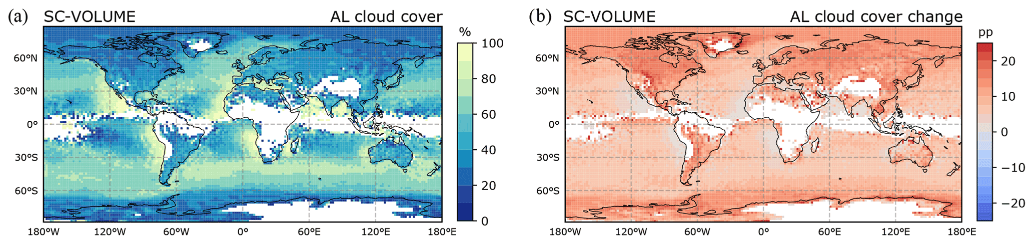
Figure 8 Mean (a) cloud cover and (b) cloud cover change in the ambiguous layer with SC-VOLUME, conditionally sampling cases in which the ambiguous layer contained a cloud.

Table 3 Global and regional averages of mean ambiguous layer cloud cover (clc^kinv) and its increase in SC-VOLUME, conditionally sampling cases in which the ambiguous layer contained a cloud.

To assess the maximum effect that a scheme such as invgrid in SC-VOLUME, increasing the cloud cover for existing stratocumulus clouds, could cause, we performed the SC-MAX experiment. In this simulation, the cloud cover of identified stratocumulus clouds (i.e. the first cloudy layer at or below the inversion level) is set to 100 %. The SC-MAX method is also applied to those stratocumulus situations that SC-VOLUME could not affect (in which the cloud and the inversion are not in the same layer). Hence, the SC-MAX method exerts the maximum possible stratocumulus cloud cover increase.

The annual mean total cloud cover difference that is produced for the radiation routine with SC-MAX is very large, as can be seen in Fig. 6g. Further, in this case, the changes exerted propagate through feedback much more evidently and can be clearly observed in the model's simulated total cloud cover. When comparing it to REF (Fig. 6h), the increase exhibited in the subtropical stratocumulus regions is significant. However, the model's bias compared to observations is still far from being completely corrected, as the average underestimation in the South American region, which experienced the most improvement, is still −11.7 pp with SC-MAX as opposed to −13.5 pp in REF.

The SC-MAX experiment demonstrates that a stratocumulus cloud cover scheme applied only in the radiation routine can have a positive effect on the model via feedback, but, in the case of ECHAM-HAM, it is not sufficient to fully close the gap between the simulated and observed cloud cover. Even the cloud cover seen by the radiation routine is still underestimated in the stratocumulus regions compared with the observed climatology. This experiment further confirms that ECHAM-HAM's cloud cover bias is caused also by a lack of stratocumulus clouds in the first place. A scheme such as SC-VOLUME can only correct the cloud cover when a cloud is already present, and, as such, it has limited effectiveness when the main model bias is the frequency of cloud occurrence. The implementation of a scheme affecting only existing clouds, such as SC-VOLUME, would need to be complemented by improvements in other parameterisation schemes to increase the occurrence of stratocumulus clouds as well. It would be better suited for models that correctly simulate stratocumulus frequency but have overly low cloud cover when present.

The SC-SUND scheme presents a possible improvement to this, as it can be applied even in columns with no below-inversion cloud at all, with the possibility to form a new cloud there.

3.3.3 New clouds in SC-SUND

The SC-SUND scheme has the potential to address both of the issues identified in the previous sections in the SC-VOLUME set-up, namely its inability to address cases in which the stratocumulus is below the inversion layer and the scarcity of simulated stratocumulus in the model. It can form a “new cloud” when the Sundqvist scheme diagnoses positive cloud cover in a layer on the new grid which previously had zero cloud cover but some condensate.

Figure 9a shows the frequency of occurrence of a cloud in the ambiguous layer after SC-SUND's reconstruction, and Fig. 9b displays its increase compared with the original representation. The SC-SUND scheme forms new clouds up to 30 % of the time in the southern marine subtropical stratocumulus regions, also significantly extending the area over which the condition occurs over the ocean. This demonstrates that the separation of the PBL and free troposphere achieved with the refined grid is very effective and allows clouds that could not be formed previously in the coarser grid box to be “revealed” on a re-execution of the cloud cover scheme. The overall effect that a newly formed cloud in the ambiguous layer has on total cloud cover depends on the presence of a cloud in other layers: in a previously cloud-free column, a new cloud generally increases the total cloud cover more significantly than in a column already containing a cloud.

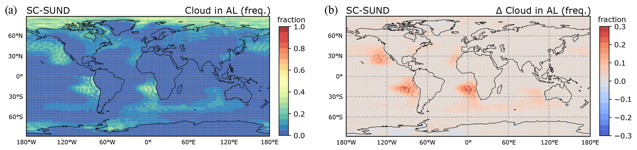
Figure 9 Presence of a cloud in the ambiguous layer in the SC-SUND simulation: (a) frequency (cf. Fig. 7c) and (b) frequency increase compared with prior to the application of SC-SUND.

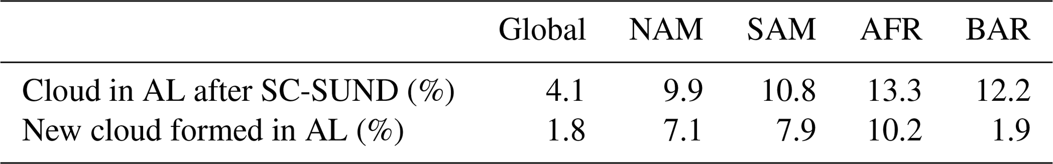
Table 4 Global and regional averaged occurrence frequency in the SC-SUND simulation of having a cloud in the ambiguous layer and of forming a new cloud in the ambiguous layer.

The total cloud cover change experienced in the annual mean by the radiation routine in the SC-SUND simulation is quite large, reaching up to 15 pp in some columns and affecting extended areas (Fig. 6e). It is of comparable magnitude to that in the SC-MAX simulation (Fig. 6g). However, it is interesting to note that the effect that is then produced on the simulated total cloud cover is much less marked with SC-SUND than with SC-MAX (see Fig. 6f and h). In fact, the process by which the annual mean total cloud cover seen by the radiation routine is increased is different in the two set-ups. In SC-MAX, the annual mean increases because all simulated stratocumulus clouds reach 100 % coverage, but their number remains the same. In SC-SUND, it increases because the scheme can form new clouds; hence, stratocumulus clouds appear more frequently, with their coverage being calculated as usual. Thus, in SC-MAX, sunlight is almost fully scattered back to space in all situations with a stratocumulus cloud, which can have a very drastic effect on the radiation balance in stratocumulus regions; in contrast, in SC-SUND, the increase in short-wave scattering in stratocumulus regions is more evenly distributed over time and may therefore produce a more moderate effect on the meteorological conditions in those regions.

The reason that the effect produced in SC-SUND is weaker may be because the new clouds occurring in the scheme, although they have a more realistic cloud cover, are likely to have an overly low liquid or ice content. Their liquid or ice content comes from the condensation or deposition computed using the original grid's grid box mean RH (i.e. at low supersaturation) or from transport – both resulting in low amounts. This is a disadvantage of SC-SUND, as to have a realistic liquid or ice content, the grid refinement should also be applied in the cloud microphysics scheme.

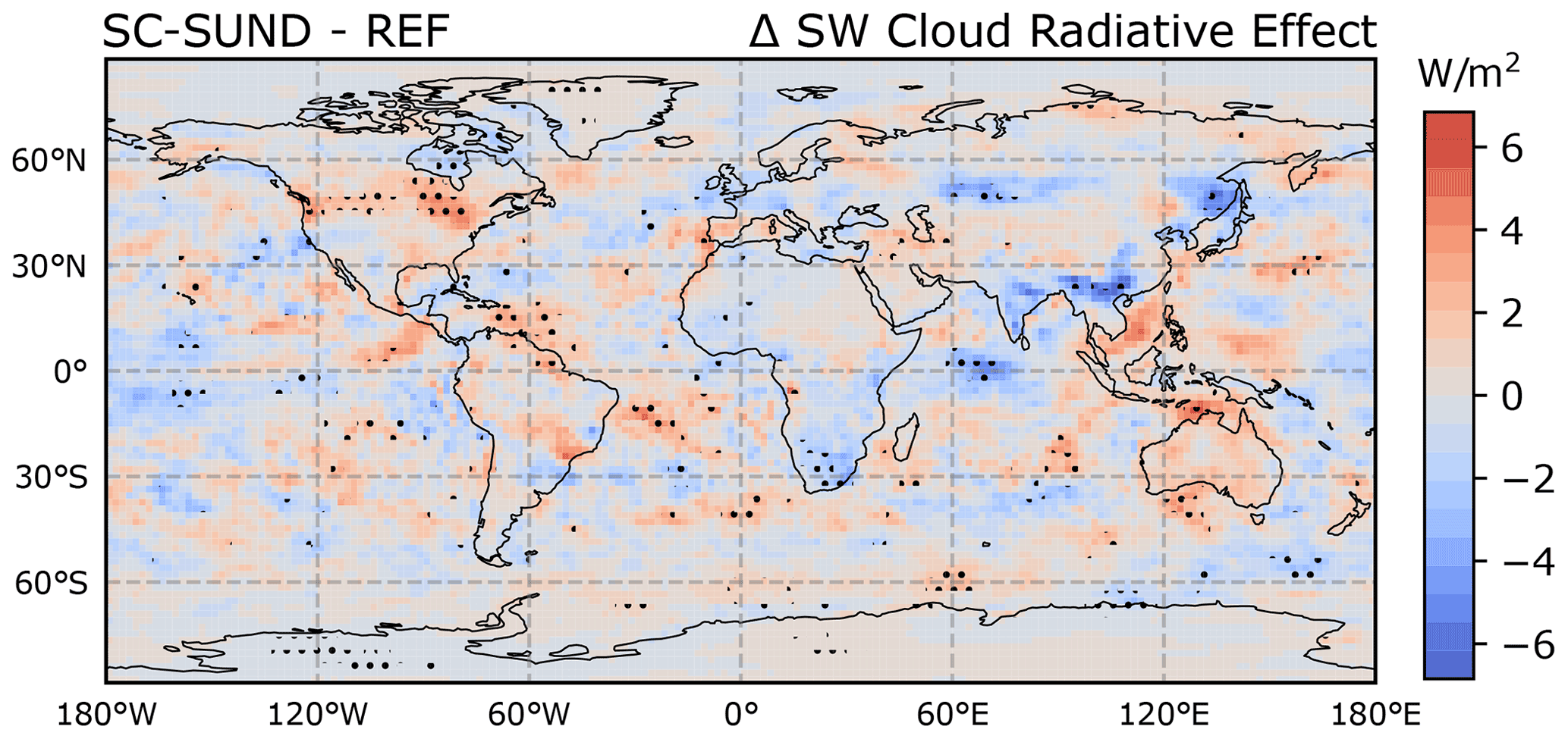
To test this explanation, we evaluated the difference in the short-wave (SW) cloud radiative effect (CRE) between the REF and SC-SUND simulations, which gives us information about whether the new clouds formed in SC-SUND are radiatively different from the “original” ones in REF. As the CRE is the difference between all-sky and clear-sky radiative fluxes, its magnitude can change based on changes in cloud cover, cloud occurrence frequency, or cloud optical thickness. A more negative CRE can be expected in stratocumulus regions in SC-SUND, as both cloud cover and cloud frequency increased in the radiation routine, as long as the cloud optical thickness is large. Figure 10 shows the difference in mean SW CRE between the REF and SC-SUND simulations. Stippling shows regions where the difference is statistically significant at the 95 % significance level. In stratocumulus regions, where an important increase in mean cloud cover was simulated (Fig. 6e), the SW CRE difference is still not significant. This can only be explained if the mean optical thickness of newly formed clouds, primarily responsible for the mean cloud cover increase in the radiation scheme in SC-SUND, was abnormally low and close to zero. This provides an explanation as to why the application of SC-SUND only in the radiation routine did not have the desired effect despite the large increase in cloud cover and occurrence – as suggested, the newly formed clouds are devoid of significant cloud condensate and, hence, are not radiatively active. If the new clouds were comparable to the pre-existing clouds in terms of water condensate, a strong radiative change would be observed, leading to favourable feedback, like in SC-MAX.

Figure 10 Short-wave (SW) cloud radiative effect difference between the REF and SC-SUND simulations. Stippling indicates statistically significant differences at the 95 % significance level; the false discovery rate is controlled following Wilks (2016).

These results indicate that the cloud cover improvement obtained in the radiation routine thanks to the implementation of invgrid is “lost”, as the radiative impact is too weak for the changes to be propagated to the simulated climate, due to an overly low water content in the new clouds. Despite the higher complexity, it may be beneficial to extend the grid refinement scheme directly to the cloud-related microphysics and cover routines in order to simulate a better representation of the cloud condensate and obtain a sizable improvement in ECHAM-HAM's simulated stratocumulus clouds.

4 Summary and conclusions

Two parameterisations for stratocumulus cloud cover based on a vertical grid refinement at the level of the capping inversion were developed and implemented only in the radiation routine of ECHAM-HAM GCM. SC-VOLUME uses a geometrical and physical argument to augment the cloud's horizontal extent under the inversion; SC-SUND makes use of the improved temperature and water profile at the inversion and re-evaluates the cloud cover.

The inclusion of SC-VOLUME did not lead to significant improvements in the model's cloud cover bias in long-term global climate simulations. Our investigation into the reasons behind this lack of sensitivity (whereas other similar schemes that were also only implemented in the radiation routine have led to improvements in other models, e.g. Boutle and Morcrette, 2010) revealed interesting new insights into ECHAM-HAM's stratocumulus bias that we believe could also be relevant for other models.

Firstly, the simulated stratocumulus clouds only very rarely occur in the model layer containing the inversion and, instead, more often appear in a lower layer. This shows a systematic bias in the model's representation which may be due to the poor resolution of the humidity profile not permitting the formation of a cloud in the inversion layer. As the correspondence of the inversion layer and cloud layer is a necessary condition for the application of SC-VOLUME's cloud squeezing method, this means that the scheme can only be applied in a small fraction of the identified stratocumulus cloud cases, limiting its general effect. Having identified this common stratocumulus–inversion layer mismatch is valuable, as it explains why a geometry-based method for the representation of stratocumulus clouds such as SC-VOLUME is not widely applicable in ECHAM-HAM and suggests that it would work better with a higher vertical resolution – which would improve stratocumulus cover representation regardless.

Secondly, the SC-MAX experiment showed that even if the cloud cover of all stratocumulus clouds in the model was 100 %, the model's mean cloud cover in stratocumulus regions would still be too low compared with observations. This demonstrates that the model's stratocumulus cover bias is not only due to an underestimation of simulated clouds' horizontal extent but also to an underestimation of their occurrence frequency and the areas where they appear, i.e. the cloud formation mechanisms are insufficiently parameterised in the first place. Hence, we conclude that a method like SC-VOLUME, which addresses and attempts to correct only the cloud amount of pre-existing clouds, is too limited to close the gap.

The SC-SUND scheme aimed to address both of the issues limiting SC-VOLUME. In fact, its application led to the formation of new clouds in the refined below-inversion grid layers and, hence, to a larger increase in the total cloud cover seen by the radiation routine compared with SC-VOLUME. However, this positive effect was not propagated to the simulated cloud cover in a significant form through feedback driven by changes in CRE. We showed that the likely reason is that the liquid water content in the newly formed clouds is too low, as it has not been recalculated with the proper microphysics routine on the new grid. Here as well, the model's original insufficient representation limits the effectiveness of the scheme – despite its numerical advantages, the implementation of a stratocumulus cloud parameterisation limited to the radiation routine is mostly unprofitable.

As the developed grid refinement method itself works well and improves stratocumulus cloud cover within the radiation routine, where it is currently applied, it could be valuable in the future to expand its use to other parts of the model as well. In particular, as a further step, the grid refinement could be applied in the cloud microphysics and cloud cover routines. There, the refined grid would lead to an improved reconstruction of the water content profile around the inversion and representation of some stratocumulus-related processes, consolidating the improvements in cloud cover. We think that this implementation could be sufficient for model performance improvements, seeing e.g. the radiation-only implementation of Boutle and Morcrette (2010). However, it is also possible that we might then wish to expand the grid refinement scheme to the vertical mixing to further improve the representation. At that point, a full PBL parameterisation such as that presented in Grenier and Bretherton (2001) or Bretherton and Park (2009) may be a neater solution.

The choice of a way forward should also be weighed against the more straightforward option of increasing the vertical resolution throughout the model: it is difficult for simple parameterisations to generate a better representation when the underlying state is flawed due to poor resolution. This would be “safer” as it would not involve approximations made when parameterising physical processes, and it would also be beneficial for phenomena other than stratocumulus clouds, such as convection. The commonly cited disadvantage of this approach is the computational cost, which is proportional to the number of grid layers. Moreover, having a variable interface level matching the inversion and, hence, allowing for more variable PBL heights has the potential to better represent real situations. It is advantageous for the physics both in terms of cloud location and vertical mixing across the PBL, compared with just having more (but fixed) levels (e.g. Suarez et al., 1983).

Finally, and perhaps most simply, the Sundqvist cloud cover scheme used in ECHAM-HAM is simply not suited for layers representing different air masses with distinct properties, such as those around the inversion in a stratocumulus-capped marine PBL. It tends to underestimate the cloud cover that would be expected from the moist part, as it assumes the grid box mean RH is representative of uniform layer conditions. Recently, Weverberg et al. (2021b) developed a cloud cover parameterisation ideally suited to these situations: the cloud fraction and water content are derived from a bimodal probability distribution function representing the sub-grid saturation variations, with a dry and a moist mode. The scheme improves several cloud properties in regional simulations compared with schemes assuming a unimodal PDF, such as implicitly assumed in the Sundqvist scheme (Weverberg et al., 2021a). For improving stratocumulus cloud cover in ECHAM-HAM, reconsidering the cloud fraction scheme itself and updating it to a more physical one could also be a productive step forward.

Appendix A: Illustrative radiative transfer calculations with invgrid

To illustrate the radiative effect of cloud squeezing with invgrid (SC-SUND), we performed a simple radiative flux calculation. We consider only the short-wave (SW) radiative flux for simplicity, as it is the dominant factor. In ECHAM-HAM, the radiative flux through a column grid box observed at the top of the atmosphere (TOA) is

$$\begin{array}{}\text{(A1)}& {\displaystyle }{\displaystyle }{F}_{\text{allsky}}=(\mathrm{1}-b)F_{\text{clear}}+b{F}_{\text{cloud}},\end{array}$$

where b denotes the layer cloud cover. The SW cloud radiative effect (CRE) is defined as

$$\begin{array}{}\text{(A2)}& {\displaystyle }{\displaystyle }{\text{CRE}}_{\text{SW}}=F_{\text{allsky}}-F_{\text{clear}}.\end{array}$$

We calculate the clear-sky and cloudy short-wave fluxes using radiative transfer equations from Corti and Peter (2009):

$$\begin{array}{}\text{(A3)}& {\displaystyle }& {\displaystyle }{F}_{\text{clear}}^{\text{SW}}\approx I_{\mathrm{0}}\left(\mathrm{1}-r-t{t}^{\prime }\mathit{\alpha }\right),\text{(A4)}& {\displaystyle }& {\displaystyle }{F}_{\text{cloud}}^{\text{SW}}\approx I_{\mathrm{0}}\left(\mathrm{1}-r-t{t}^{\prime }\mathit{\alpha }-\left(\mathrm{1}-\mathit{\alpha }\right)t{t}^{\prime }{\displaystyle \frac{R_{\mathrm{c}}-\mathit{\alpha }{R}_{\mathrm{c}}^{\prime }}{\mathrm{1}-\mathit{\alpha }{R}_{\mathrm{c}}^{\prime }}}\right),\end{array}$$

where I₀ is the incoming solar flux, r is the atmospheric reflectivity, tt^′ is the product of downward and upward atmospheric transmittance, α is the surface albedo, and R_c and $R_{\mathrm{c}}^{\prime }$ are the cloud reflectances for incoming and outgoing radiation respectively. The latter parameters are calculated as

$$\begin{array}{}\text{(A5)}& {\displaystyle }& {\displaystyle }{R}_{\mathrm{c}}\approx {\displaystyle \frac{\mathit{\tau }/\mathit{\zeta }}{\mathit{\gamma }+\mathit{\tau }/\mathit{\zeta }}},\text{(A6)}& {\displaystyle }& {\displaystyle }{R}_{\mathrm{c}}^{\prime }\approx {\displaystyle \frac{\mathrm{2}\mathit{\tau }}{\mathit{\gamma }+\mathrm{2}\mathit{\tau }}},\end{array}$$

where τ is the cloud optical depth, $\mathit{\gamma }=\mathrm{1}/(\mathrm{1}-g)$ and g is the asymmetry factor, and ζ is the cosine of the solar zenith angle (SZA).

In our calculations, the values used for the parameters are r=0.15, $t{t}^{\prime }=\mathrm{0.73}$, and γ=0.77 (Corti and Peter, 2009); α=0.05 for the ocean; $\text{SZA}=\mathrm{45}{}^{\circ }$; and I₀=1360 W m⁻² (solar constant).

We use τ=12 and b=0.6 as an example. If the layer thickness Z is reduced by one-third with invgrid ($Z^{\text{ig}}/Z=\mathrm{2}/\mathrm{3}$), we obtain $b^{\text{ig}}=b\cdot Z/Z^{\text{ig}}=\mathrm{0.9}$ and ${\mathit{\tau }}^{\text{ig}}=\mathit{\tau }\cdot b/b^{\text{ig}}=\mathrm{8}$ on the refined grid (denoted with superscript ig). The resulting all-sky fluxes and SW CRE are

$$\begin{array}{}\text{(A7)}& {\displaystyle }& {\displaystyle }{F}_{\text{allsky}}\approx \mathrm{724}\mathrm{W}{\mathrm{m}}^{-\mathrm{2}},\text{(A8)}& {\displaystyle }& {\displaystyle }{F}_{\text{allsky}}^{\text{ig}}\approx \mathrm{613}\mathrm{W}{\mathrm{m}}^{-\mathrm{2}},\text{(A9)}& {\displaystyle }& {\displaystyle }{\text{CRE}}_{\text{SW}}\approx -\mathrm{382}\mathrm{W}{\mathrm{m}}^{-\mathrm{2}},\text{(A10)}& {\displaystyle }& {\displaystyle }{\mathrm{CRE}}_{\mathrm{SW}}^{\mathrm{ig}}\approx -\mathrm{493}\mathrm{W}{\mathrm{m}}^{-\mathrm{2}},\end{array}$$

i.e. the effect of cloud squeezing is a reduction in the net short-wave radiative flux at the TOA.

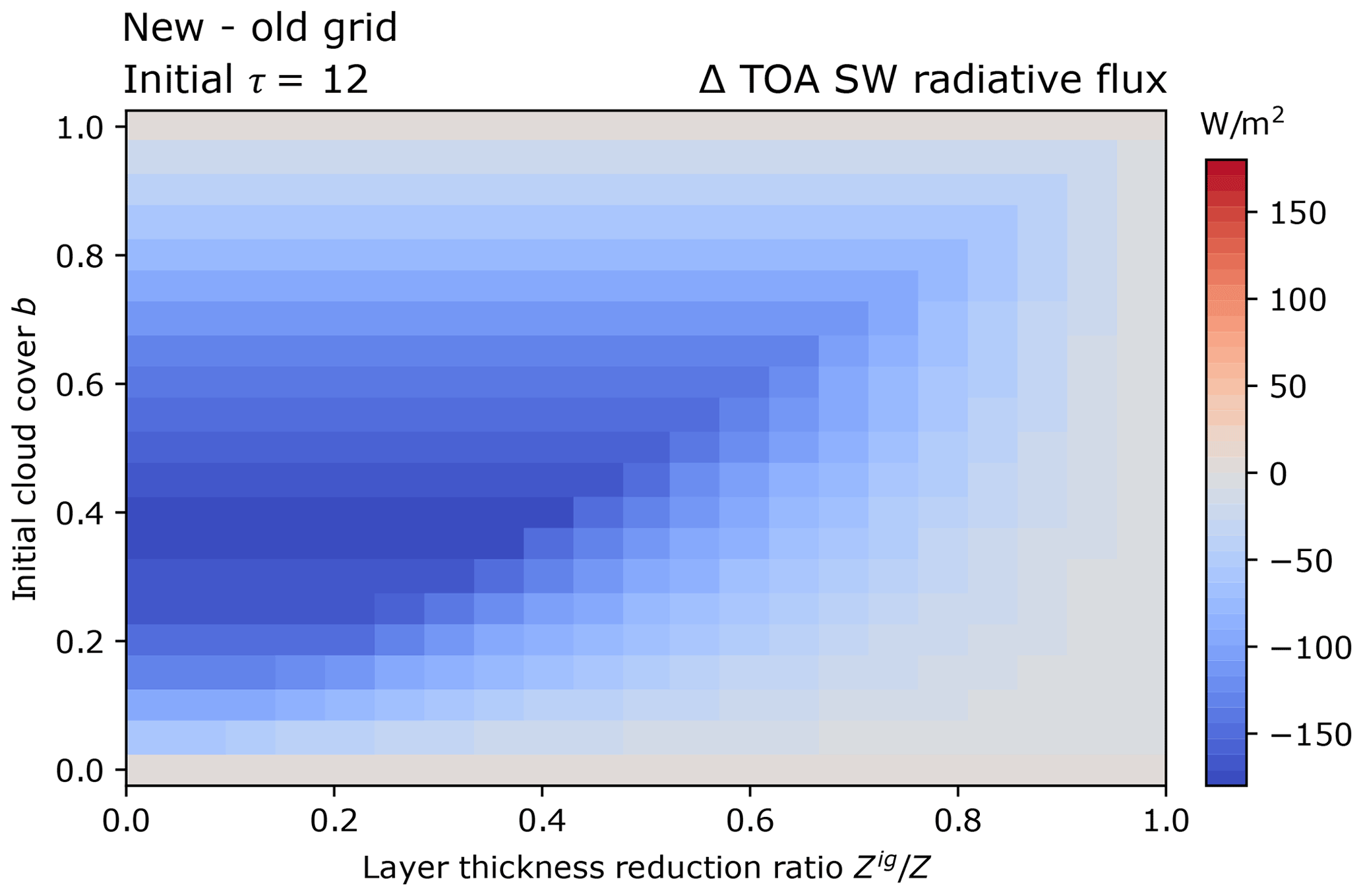
Figure A1 Change in short-wave (SW) radiative flux due to the application of SC-VOLUME cloud squeezing for a cloud with an initial τ=12, varying initial cloud cover values as on the y axis, and varying thickness reduction ratios as on the x axis.

Figure A1 shows the difference between new- and old-grid short-wave radiative flux, as a function of initial layer cloud cover and layer thickness reduction ratio. Applying the SC-VOLUME scheme can be seen to always have a negative (or at most zero) SW radiative effect. From the results presented in Table 3, the affected layers in stratocumulus regions have initial values of b=0.75 and $Z^{\text{ig}}/Z=\mathrm{0.95}$ in SC-VOLUME on average. Under these conditions, with an initial value of τ=12, as in Fig. A1, the SW radiative effect would be relatively small, at around −20 W m⁻².

Appendix B: Modified EPIC SCM experiments

We ran the EPIC SCM experiment with modified forcing conditions and perturbed initial fields to further test the performance of the inversion reconstruction method. In our main EPIC SCM simulations, the measured values of the vertical temperature and humidity profiles were used in the model at every time step (“fully forced”). This allowed us to focus on analysing the performance of the inversion reconstruction scheme while being minimally biased by the SCM's ability to accurately reproduce a situation from a forcing. With this set-up, a perturbation of the initial conditions (as in Hack and Pedretti, 2000) would dissipate in a few time steps. Therefore, for the perturbation experiments, we weakly nudged the SCM instead, with a relaxation timescale τ_x of 5 h for temperature and humidity (see Eq. 25 in Lohmann et al., 1999). The initial temperature and absolute humidity fields were perturbed following Hack and Pedretti (2000) (i.e. a normal additive perturbation with a standard deviation of 0.5 K and absolutely bounded by 0.9 K for the temperature, and a multiplicative perturbation such that the standard deviation is 0.5 g kg⁻¹ in the boundary layer and absolutely bounded by 6 % for the absolute humidity). The experiment with τ_x=5 h was run 50 times with different perturbed initial conditions. With this nudging set-up, perturbations in the initial conditions can lead to differences in the reconstructed inversion height throughout the duration of the simulation.

The results are shown in Fig. B1. Compared with the previous fully forced simulation, the results appear less accurate at times, with more frequent sudden “jumps”, particularly around the day 3. However, the reconstructed inversion height is well in line with the observed cloud top during the first 2 and last 2 d. When the initial conditions are perturbed, the results for the inversion height deviate from the unperturbed simulation mostly during day 1, with only a few also deviating around days 4 and 5. Overall, despite the evolution being more weakly forced, the reconstructed inversion height remains mostly consistent. This suggests that the inversion reconstruction method is robust.

In Table B1, some statistical characteristics of the simulations are given. Note that the percentage of the time the inversion is successfully reconstructed remains constant across the simulations because the stability criterion used also depends on the large-scale subsidence, which is unaffected by τ_x or by the perturbations in temperature and humidity, which in the case of the EPIC SCM experiment proves to be the limiting factor.

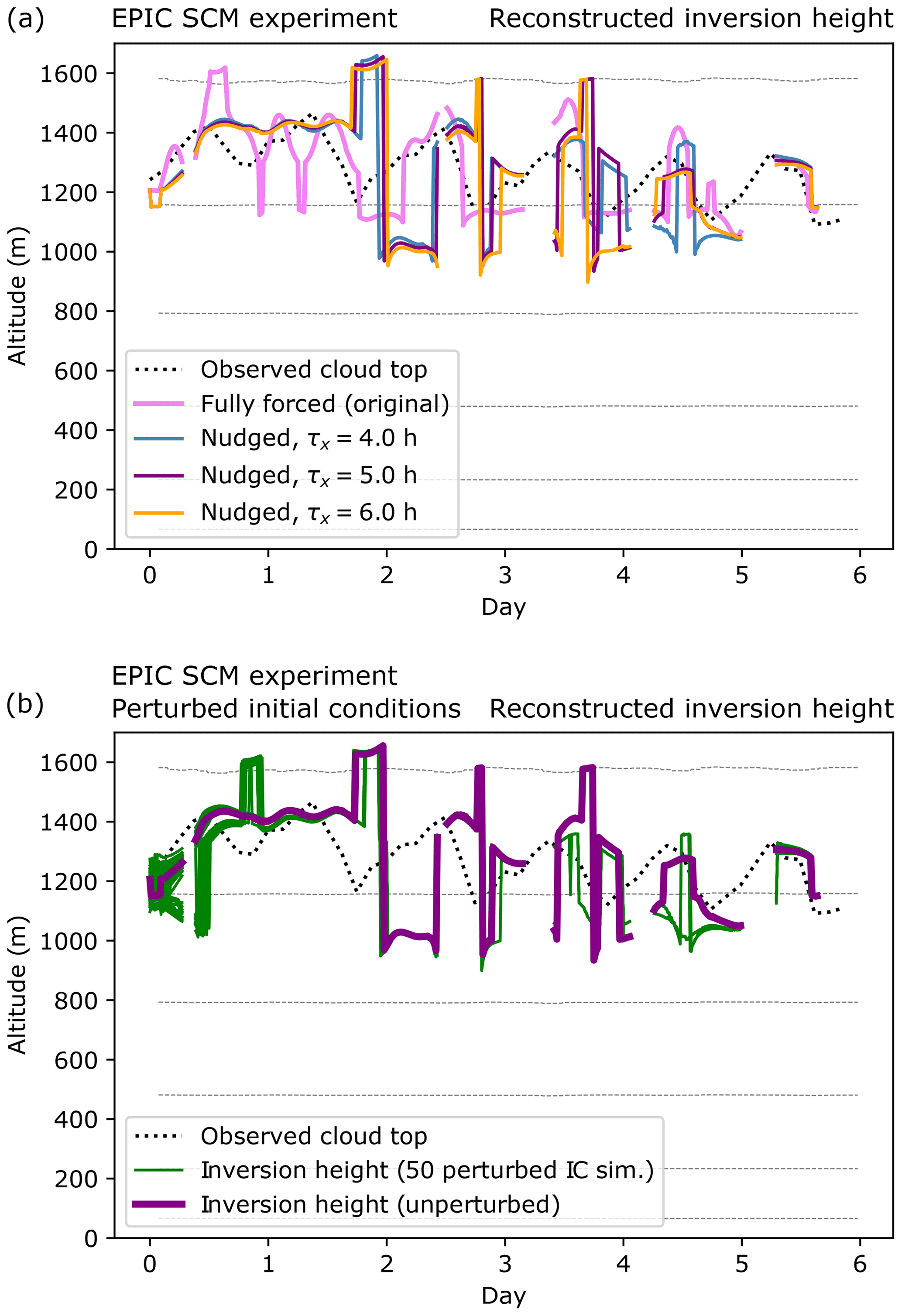
Figure B1 Reconstructed inversion heights in modified EPIC SCM experiments (a) with different nudging relaxation timescales τ_x and (b) with τ_x=5 h and perturbed initial conditions.

Table B1 Results from the modified EPIC SCM experiments: percentage of the time that the inversion is reconstructed, and the mean and standard deviation (SD) of the mismatch (absolute difference) between the reconstructed inversion height z_inv and the measured cloud top (linearly interpolated to all model time steps). Results are presented for the fully forced simulation; nudged simulations with τ_x of 4, 5, and 6 h; and for the lower and upper quartiles of the 50 perturbed simulations of the τ_x=5 h experiment.