the Creative Commons Attribution 4.0 License.
the Creative Commons Attribution 4.0 License.
 | 18 Aug 2021
Hydrostreamer v1.0 – improved streamflow predictions for local applications from an ensemble of downscaled global runoff products
Joseph H. A. Guillaume
Vili Virkki
Matti Kummu
Kirsi Virrantaus
An increasing number of different types of hydrological, land surface, and rainfall–runoff models exist to estimate streamflow in river networks. Results from various model runs from global to local scales are readily available online. However, the usability of these products is often limited, as they often come aggregated in spatial units which are not compatible with the desired analysis purpose. We present here an R package, a software library Hydrostreamer v1.0, which aims to improve the usability of existing runoff products by addressing the modifiable area unit problem and allows non-experts with little knowledge of hydrology-specific modelling issues and methods to use them for their analyses. Hydrostreamer workflow includes (1) interpolation from source zones to target zones, (2) river routing, and (3) data assimilation via model averaging, given multiple input runoff and observation data. The software implements advanced areal interpolation methods and area-to-line interpolation not available in other products and is the first R package to provide vector-based routing. Hydrostreamer is kept as simple as possible – intuitive with minimal data requirements – and minimises the need for calibration. We tested the performance of Hydrostreamer by downscaling freely available coarse-resolution global runoff products from the Inter-Sectoral Impact Model Intercomparison Project (ISIMIP) in an application in 3S Basin in Southeast Asia. Results are compared to observed discharges as well as two benchmark streamflow data products, finding comparable or improved performance. Hydrostreamer v1.0 is open source and is available from http://github.com/mkkallio/hydrostreamer/ (last access: 5 May 2021) under the MIT licence.
- Article
(3413 KB) - Full-text XML
- BibTeX
- EndNote


An increasing number of different types of hydrological, land surface, and rainfall–runoff models exist to estimate streamflow in river networks. Alternative models with different assumptions, model structures, and process representations increase the options to address specific hydrological problems. Using these models, however, requires skill and training to overcome barriers that inexperienced modellers or non-experts often face; for instance, hydrological jargon (Venhuizen et al., 2019), hydrological textbooks focusing on equations (Shaw et al., 2019), the curse of equifinality (Beven, 2006), selection of model performance indicators (Krause et al., 2005), selection of an appropriate model (Addor and Melsen, 2019; Singh and Woolhiser, 2002), and data collection, among others (Brunner et al., 2021). A non-expert (by which we mean a person who is interested in hydrological information but is not an expert in hydrological modelling) has several options to choose from when facing this problem. They can, for instance, seek help of an expert hydrologist, possibly incurring costs to their project, or delayed delivery if parts of the project need to wait for input from the hydrologist. Or they can apply a model with simplified process representations or which are designed for teaching. These models include, e.g. a simple rainfall–runoff ratio, Khosla's method (Subramanya, 2017), HBV (Seibert and Vis, 2012), or airGR (Delaigue et al., 2018), all of which still require data collection and calibration or obtaining parameter estimates from an external source. Using a model evaluation framework (e.g. Hamilton et al., 2019), an inexperienced hydrological modeller may in this case encounter challenges relating to impacts at project level (efficiency, credibility, salience, accessibility) and group level (application and satisfaction).
Alternatively, the non-expert can use readily available hydrological data products prepared by expert teams, sidestepping many of the aforementioned issues. The drawback of using off-the-shelf existing products is that they often come aggregated in spatial units which are not compatible with the desired analysis purpose. This issue is termed the modifiable area unit problem (MAUP) – a statistical bias in analyses arising from arbitrarily defined aggregation zones, resulting in both a scale effect and zoning effect (Manley, 2014). The scale effect occurs when the aggregation of a statistic to different scale enumeration areas (such as catchment, basin, or watershed) produces different statistics. The zoning effect occurs when different arrangements of enumeration areas (such as a regular grid and a polygon-type administrative area) produce different values for the same sample location. If MAUP is not addressed during an analysis, the analyst runs a risk that the data used are not representative of their units of analysis. Salmivaara et al. (2015) explore MAUP for water resource assessments in more detail.
A number of options to address MAUP have been developed (Dark and Bram, 2007), but no comprehensive solution has been found. Solutions range from simply ignoring MAUP to analysing each elementary areal unit relevant for the variable or process. However, ignoring the problem and hoping for the best does not seem like a desirable solution, and analysis of every possible elementary unit may not be computationally feasible. One of the solutions is to use some areal interpolation method to estimate variable values in alternate aggregation zones (Kar and Hodgson, 2012). Such areal interpolation methods include any method which estimates an unknown variable value in a target zone based on known values in a source zone (Goodchild and Lam, 1980). In the context of hydrological modelling, a considerable body of literature exists for statistical interpolation of hydrological variables to ungauged basins (e.g. Gottschalk, 1993; Lehner and Grill, 2013; Paiva et al., 2015; Parajka et al., 2015; Skøien et al., 2006). Process-based interpolation has gained little attention outside our previous work (Kallio et al., 2019) and that of Kar and Hodgson (2012), who propose a method of incorporating process understanding in application of advanced areal interpolation methods for downscaling runoff and for estimating population densities, respectively.
Notwithstanding the issues with MAUP, the workflow of estimating discharge from runoff remains similar. Regardless of the method used to estimate runoff, once the quantity of runoff is approximated for a certain area, discharge is commonly derived by applying a river-routing algorithm which accumulates the runoff down a river network. Distributed and semi-distributed hydrological models often have a built-in routing component. Nevertheless, hydrological variables are also modelled by land-surface models and dynamic vegetation models, which may require coupling with a routing model. A number of software solutions exist which first interpolate runoff to arbitrary river reaches and apply various routing methods, either on a node–link network or between grid cells representing the river system. Focusing here on node–link networks, examples of such tools are Routing Application for Parallel computatIon of Discharge (RAPID; David et al., 2011), mizuRoute (Mizukami et al., 2016), and HYDROROUT (Lehner and Grill, 2013). While these tools do include a step to map runoff products onto the river network, their focus is primarily on routing (RAPID and MizuRoute are high-performance solutions), with interpolation limited to centroids and simple area-weighted interpolation.
Furthermore, many authors have recognised the need for multiple estimates for robust problem solving in hydrology (e.g. Addor and Melsen, 2019; Blair and Buytaert, 2016) using alternative model structures, assumptions, and source datasets. This is currently not explicitly handled in available interpolation and routing tools. The inclusion of several estimates is commonly achieved through uncertainty quantification (Vrugt and Robinson, 2007), but when using existing source datasets, these typically represent a sample of convenience, and it may be of limited use to focus on uncertainty across interpolation methods. Instead, it makes sense to treat the use of multiple estimates as a model selection problem or more generally, a model averaging (MA) problem, where predictive performance dictates which methods to select or their contribution to a combined prediction (Diks and Vrugt, 2010). Performance is expected to vary spatially and temporally, and observation data are not available for all cases, so methods are then also needed to select models in areas without performance information. MA can additionally contribute to solving MAUP, where estimates from alternative zonings are used as inputs for MA. Such alternative zonings in the context of water resource assessments may be different realisations of uncertain drainage basin delineations (Eränen et al., 2014) or combinations of physical and administrative delineations (Salmivaara et al., 2015).
This paper responds to the need for downscaling of existing runoff products in a way that addresses the MAUP, links to routing functionality, and allows for use of model averaging on an ensemble of convenience. Further, the use of existing runoff products relaxes the requirements for hydrological modelling expertise from the user's part, provided that they possess the expertise in R programming and elementary skills in working with spatial data. The software introduced presents an alternative to existing software tools to provide further options to tackle the scale effect (downscaling, upscaling) and zoning effect (similar resolution, but non-conforming zones) of the MAUP. Hydrostreamer v1.0, a software library written in the R language (R Core Team, 2019), uniquely combines (1) advanced areal interpolation methods, (2) lateral routing methods, and (3) functions for data assimilation via a model averaging approach in order to improve and extend the usability of off-the-shelf runoff products. Hydrostreamer particularly implements advanced areal interpolation methods: (1) dasymetric mapping (DM), areal interpolation which is guided by ancillary variables (Comber and Zeng, 2019; Eicher and Brewer, 2001; Wright, 1936), and (2) pycnophylactic interpolation (PP), a technique to estimate internal variable distribution within a specified zone (Tobler, 1979). To our knowledge, there are currently no other software solutions for R which implement DM, but area-weighted interpolation is available in at least sf (Pebesma, 2018) and areal (Prener and Revord, 2019) R packages. Tobler designed PP for an internal representation using a square grid scheme, and Rase (2001) developed an adaptation of PP for triangulated irregular networks. To the best of our knowledge, Hydrostreamer is the first software package which implements PP for polygon networks as the internal representation, but a gridded version is available for R in package pycno (Brunsdon, 2014). Hydrostreamer also implements an area-to-line interpolation which supports using river networks obtained from mapping surveys or topographic databases as an alternative to networks extracted from digital elevation models, which can be highly uncertain (Lindsay and Evans, 2008).
We demonstrate the capabilities of Hydrostreamer with a case study in the data-poor 3S basin in Southeast Asia. The 3S basin is a major tributary of the Mekong River, consisting of the three rivers Sekong, Sesan, and Srepok under southwest monsoon climate. In the case study, we use Hydrostreamer to downscale 15 runoff products obtained from the Inter-Sectoral Impact Model Intercomparison Project (ISIMIP; simulation experiment 2a; Gosling et al., 2017) onto the HydroSHEDS river network (Lehner et al., 2008). Following this, we route the downscaled runoff down the river network and perform model averaging against streamflow records from 10 monitoring stations. Performance of streamflow predictions against gauged observations is compared with benchmarks of a recent streamflow product, GRADES (Global Reach-Level A Priori Discharge Estimates for SWOT; Lin et al., 2019), and ECMWF published global streamflow reanalysis product, GLOFAS (GLObal Flood Awareness System; Alfieri et al., 2020).
The rest of the paper is structured as follows. In Sect. 2 we introduce the four steps of preprocessing, areal interpolation, routing, and model averaging in Hydrostreamer. In Sect. 3 we introduce the software architecture. Section 4 describes the case study method, data, and experiments, for which the results and discussion are provided in Sect. 5. Section 6 discusses future development plans, and Sect. 7 gives conclusions.
Hydrostreamer is designed as a complete solution from preprocessing source data to interpolation, river routing, post-processing outputs, and evaluating model performance. It is written in the R language (R Core Team, 2019), which is receiving increasing attention in the hydrological sciences (Slater et al., 2019). We have aimed to keep the core functionality of the package as simple as possible to facilitate its use for non-experts while implementing enough functionality to also be useful for the hydrological community. Figure 1b shows the generalised steps taken in a typical Hydrostreamer workflow. This section is structured as follows: obtaining data and preprocessing are discussed in Sect. 2.1, interpolation methods (Step I) are described in Sect. 2.2, river routing (Step II) is discussed in Sect. 2.3, and data assimilation by model averaging (Step III) is discussed in Sect. 2.4.

Figure 1(a) Study area and the data used in the empirical study: runoff from global hydrological models at 0.5∘ resolution, a river network, and monitoring data. (b) The three steps in a typical Hydrostreamer workflow. Step I: areal interpolation, or area-to-line interpolation, to distribute runoff from source zone to target zones (or river lines). Step II: river routing. Step III: model averaging to create a multi-model combination (and regionalisation) if data from monitoring stations are available.
2.1 Obtaining data and preprocessing
Hydrostreamer has been designed to work with very low data requirements consisting of, at minimum, a distributed runoff dataset as the source zones and an explicit river network as the target zones, both of which can be obtained from free and open repositories. Additional data in the form of a digital elevation model (DEM) or ancillary information on the target river network can be used to further improve the streamflow estimates.
Hydrostreamer is designed to take runoff in a raster time series format – a multi-layer raster where each layer corresponds to a specific time step – as a plug-and-play solution. Such datasets include, for instance, LORA (Linear Optimal Runoff Aggregate; Hobeichi et al., 2019) and GRUN (Ghiggi et al., 2019), both of which are optimised global runoff datasets at 0.5∘ resolution. Outputs of a large number of global hydrological and land-surface models can also be obtained from the ISIMIP archive (as is done in the case study described in Sect. 4; https://www.isimip.org/, last access: 5 May 2021) at the same 0.5∘ resolution. In order to use this type of data in Hydrostreamer, one needs to read it in the R session, and use the raster_to_HS() function to format the data for Hydrostreamer to use. Non-gridded data may also be used, and one potential source dataset is GRADES (Lin et al., 2019), which is used as a benchmark dataset in this study. While Hydrostreamer supports non-gridded input runoff via the function create_HS(), its use may not be trivial and depending on the source format may require additional preprocessing steps.
The river network required by Hydrostreamer can be obtained from various sources. Any network which is topologically clean can be used as a plug-and-play solution without any preprocessing needed when Step I (Figs. 1 and 2) is applied. A clean network refers to a network where connected lines share a node and lines are split at junctions so that connected line segments start or end at a shared node. With a clean network, the river_network() function is able to extract the topological relationships Hydrostreamer needs. Further, if the used river network product contains topological information on the next river segment, the cleanliness requirement can be relaxed. The case study presented in Sect. 4 uses the HydroSHEDS river network (Lehner and Grill, 2013), available from https://www.hydrosheds.org/ (last access: 5 May 2021), which is an example of a clean river network. The HydroSHEDS website provides additional river network datasets with a large amount of attribute information describing each segment: Global River Classification (Dallaire et al., 2019) and HydroATLAS (Linke et al., 2019). These two datasets are particularly useful in Hydrostreamer, because their attribute information can be (but is not required) used as ancillary variables in dasymetric mapping (DM; see the following Sect. 2.2).
Hydrostreamer further provides an optional auxiliary function create_river() which can be used to extract a river network and catchment areas from a DEM for each river segment. The function requires an external program, SAGA GIS (Conrad et al., 2015), to be installed and requires definition of a threshold for the size of the stream (the Strahler stream order) at which point river line extraction starts. The selection of the threshold should be guided by the resolution of the source zones as well as understanding of the hydrology within the basin. We recommend visual inspection of the extracted river network as well as the corresponding catchment areas. Catchment areas can also be delineated for each individual river segment from a flow direction raster using function delineate_basin(), if the flow direction information from which the river network is derived is available. For HydroSHEDS, HydroATLAS, and Global River Classification, the flow direction information can be obtained from the same repository and can be used with the delineate_basin() function. Further, when an applicable DEM or flow direction is not available, function river_voronoi() approximates catchment areas by building a Thiessen polygon (Voronoi diagram) network from the line segments of the river network (Karimipour et al., 2013). This is particularly useful for river networks derived from surveying or from satellite measurements.
Finally, in order to use the model averaging functionality (optional, Step III in Figs. 1b and 2) of Hydrostreamer, one needs to obtain a time series of discharge measurements at gauges corresponding to the catchment of interest. We recommend obtaining time series from the authorities of administrative area(s) where the catchment is located, but when this is not possible, one can search the Global Streamflow and Metadata archives (Do et al., 2018) or the Global Runoff Data Centre (https://www.bafg.de/GRDC/EN/Home/homepage_node.html, last access: 5 May 2021) for appropriate data. Hydrostreamer requires observation data in a standard table format with columns for date and station observations in units of m3 s−1.
2.2 Step I: areal interpolation in Hydrostreamer
The first step in the core Hydrostreamer workflow is the areal interpolation step, which is also the key focus of the software package. In this section we give a brief background for the areal interpolation methods and how they are implemented in Hydrostreamer. For a more thorough overview and applications of areal interpolation methods, we recommend Comber and Zeng (2019). The current implementation in Hydrostreamer assumes that the interpolation is constant and does not change through time.
2.2.1 Area-weighted interpolation and dasymetric mapping
Areal interpolation methods have been developed in geography to represent regionally aggregated statistics in non-conforming area units and are discussed mostly in literature for population mapping (Comber and Zeng, 2019; Eicher and Brewer, 2001; Goodchild et al., 1993; Goodchild and Lam, 1980; Nagle et al., 2014; Wright, 1936). In principle, areal interpolation involves reallocation of a quantity from a source zone to intersecting target zones. The simplest form of areal interpolation is the area-weighted interpolation (AWI), where the reallocation is based on the proportion of intersecting areas, as shown in Eq. (1),
where is the estimated value of the variable of interest in a target zone t, ROs is the value in a source zone s, As is the area of the source zone, and At∩s is the area of the intersection of the target zone with the source zone. This form of areal interpolation is a standard practise in many hydrological applications.
The reallocation can, however, be guided by ancillary variables in dasymetric mapping (DM) if we know the process behind the interpolated variable, and additional variables describing the process are available. “Dasymetric” means density measuring, and DM is sometimes referred to as “intelligent areal interpolation” (Eicher and Brewer, 2001). In DM, the areal weights derived from AWI are further scaled using the values of the ancillary variable. With the added ancillary variable Vt, Eq. (1) becomes
where Vt is the value of the ancillary variable for the target zones and As∩t is the area of source zone intersecting all target zones. Vt can be any (numerical) variable which describes the distribution of the interpolated quantity within target zones. By definition, both AWI and DM are volume or mass preserving (pycnophylactic) – the quantity of the interpolated variable from a source zone is divided exactly among intersecting target zones. The variable Vt can also be substituted with a model f(RO) describing the process behind the variable being interpolated. This is called dasymetric modelling – see e.g. Kar and Hodgson (2012) or Nagle et al. (2014). The dasymetric variable(s) should be selected such that it (they) describes the distribution of runoff within each source zone. Potential variables include topographic information (elevation, topographic indices; the case study in this paper uses a topographic index as a dasymetric variable), land use, soil type, climate information (precipitation, temperature, evapotranspiration), and so on. The choice depends on the availability of data for each individual target zone as well as on the hydrological understanding of the user.
2.2.2 Area-to-line interpolation
AWI and DM both require that the target zone is reliably delineated with no significant uncertainty. To avoid this requirement, Hydrostreamer also provides both methods adapted for line features, which we call area-to-line interpolation. This is achieved by replacing a target zone's area A with target line's length L. In the context of river networks, both area and length are physical attributes of the river segment; one describing the catchment area associated with the river line and the other describing the river line itself. With this modification, Eq. (1) becomes
where is the estimated value of the variable of interest in a target line l, and Ll∩s is the length of the intersecting portion of river line l within the source zone. Similarly, Eq. (2) becomes Eq. (4):
In some combinations of river lines and source zones, the river may flow exactly along the boundary of two or more source zones. Since this portion intersects both source zones, such cases are explicitly handled by Hydrostreamer to split the contribution evenly among the source zones for the portion of river line at the boundary.
While the computation is similar, and both areal interpolation and area-to-line are pycnophylactic, areal interpolation can by definition work with a partial overlap between source and target zones (river segment lines). For area-to-line interpolation, there is no area representation of the target area, and therefore the used river network must intersect all source zones and should be represented in similar accuracy throughout each source zone. In our case study presented in Sect. 4, each source zone (a 0.5∘ grid; approximately 55 km at the Equator) intersects on average 56 river segments. As the performance difference is small between area-to-line interpolation and area-based interpolation methods (Appendix A, Table A1), this can be considered a sufficient density for source zones in this resolution (but subject to case-by-case evaluation). Further, since the individual river segment length is not directly proportional to its individual catchment area, area-to-line interpolation should only be used for sufficiently large basins, where the area of source zones entirely contained in the basin is significantly larger than the area of partially covered source zones. Based on our case study, monitoring stations with a drainage area of at least 30 000 km2 show very small performance difference between area-to-line interpolation and area-based interpolation methods (Table A1). Due to the large uncertainty in runoff distribution to individual segments, we recommend that the suitability of area-to-line interpolation be performance-evaluated on a case-by-case basis.
2.2.3 Pycnophylactic interpolation
While other interpolation methods may also be volume or mass preserving, pycnophylactic interpolation (PP) refers to a class of methods developed by Tobler (1979) to estimate the internal variation in a variable within a certain source zone. Tobler's application first subdivides a source zone into a regular grid and creates a smooth representation of the interpolated variable which preserves the volume within the source zone. The smoothing involves solving an integral in both the x and y direction, which is subject to the condition in Eq. (5) that preserves total volume ROs across the parts of target zones t within the original zone s (Kar and Hodgson, 2012; Tobler, 1979).
Rase (2001) developed an adaption of PP which uses triangulated irregular networks (TINs), where the double integral is simplified to averaging over nearest neighbours and weighting neighbours with inverse distance weighting. Hydrostreamer implements PP for polygon networks by adapting Rase's approach to the immediate neighbours of each target zone. This is achieved by iteratively alternating an averaging step and an adjustment step to satisfy the condition in Eq. (5). Adapting the approach of Rase, we get an averaging step
where N is the number of neighbours adjacent to target zone t, and ROj is the value of neighbour j. The averaging step is followed by an adjustment step, where the target zones within a source zone are scaled so that the Eq. (5) condition is met. If a target zone is at the boundary of the area of interest, the boundary condition is set as the starting value of the target zone at the beginning of PP. The boundary condition does not change with iterations, consistent with the suggestion of Tobler (1979). It should be noted that averaging over neighbours is done for density (i.e. runoff depth), but the smoothing condition is applied for volume (i.e. runoff volume across source zones) in order to satisfy the pycnophylactic property of PP.
PP cannot be used with river line features due to lack of computable area and non-trivial measures of neighbours. However, PP can be applied if drainage areas are estimated for the river network, for example using river segment-specific Thiessen polygons (Karimipour et al., 2013). Thiessen polygons for a line network can be computed with Hydrostreamer.
2.2.4 Combined pycnophylactic–dasymetric interpolation
Hydrostreamer implements a possibility to utilise a combination of PP and DM as described in Kallio et al. (2019). In the combined PP–DM method, the initial density of an interpolated variable for each target zone is first estimated with PP (instead of AWI), followed by DM. In this version, Eq. (2) becomes
where ROpp,t is the value of RO for target zone t, as initially estimated by PP. The advantage of the combination is that through PP we can model variables which are assumed smooth (e.g. precipitation) within and between source zones, and DM is used to estimate crisp processes.
2.3 Step II: river routing
The second step in a typical Hydrostreamer workflow involves routing runoff down a river network to estimate discharge. Two simple routing solutions, instantaneous routing and constant-velocity routing, as well as one more advanced routing solution, the Muskingum–Cunge method, are implemented in Hydrostreamer. More sophisticated schemes could be used by exporting interpolated runoff to other tools specialising in routing.
In instantaneous routing, discharge Q is the sum of runoff, in volume per time (e.g. m3 s−1), from all upstream catchments, as shown in Eq. (8):
Here Qi,t is the discharge at river segment i at time step t, ROi,t is the runoff contribution from the catchment area of segment i at the same time step t, and ROup,t is the runoff from a river segment upstream of segment i, at time step t. Instantaneous flow is the simplest form of river routing and has the advantage that it is intuitive. However, it assumes that all runoff generated at a time step t will drain through the entire river network within that same time step. The applicability of this assumption is therefore limited to catchments where the time step length far exceeds the maximum river network length. One can evaluate the applicability of the instantaneous routing (which in fact takes one time step) using Eq. (9):
where M is a dimensionless ratio between the time it takes for water to flow through the maximum upstream length of the river system Lup (in metres) at a maximum realistic average flow velocity Vmax (default 1 m s−1) during a time step of length s (in seconds). M can be interpreted so that, for example, when M=0.1, 10 % of the runoff generated at the most distant upstream location does not flow through the outlet within a single time step. The evaluation can be carried out using the function evaluate_instant_routing(). If M is found to be too large for the application, the constant flow velocity or Muskingum–Cunge option may be more appropriate.
The second option, constant velocity routing, assumes that water drains through the river network at a constant pace, which is the solution also adopted in routing tool HydroROUT (Lehner and Grill, 2013) and a number of global hydrological models (GHMs) (Telteu et al., 2021). The default flow velocity of 1 m s−1 is adopted in HydroROUT and LPJmL (Telteu et al., 2021). Assuming that the generation of runoff is uniformly distributed within a time step, we can think of a block of runoff moving downstream. Given a distance S covered in time τ at velocity V, the block of runoff typically finds itself spanning several river segments (depending on the segment size and time step length). The discharge in a particular segment comes from two blocks of runoff (two consecutive time steps) from each upstream segment. We calculate the number of whole time steps elapsed for the runoff to cover the distance Di,up and the fractions that will come from that time step and from the following time step. See Appendix B, Fig. B1. The process is described in Eqs. (10)–(14).
The third routing option implemented in Hydrostreamer is the Muskingum–Cunge routing algorithm (Cunge, 1969; Ponce, 2014). Muskingum–Cunge is a modified version of the original Muskingum routing method (Chow, 1959) where routing parameters k and x are derived from hydraulic data and do not require observation data to calibrate against. Full derivation and explanation of the Muskingum–Cunge routing can be found in Ponce (2014). The algorithm requires extensive user input in the form of river cross sections (i.e. shape, channel width, flow depth), river bed roughness (Manning's roughness coefficient), and river bed slope, which are commonly available only for certain locations. Consistent with the desire to minimise data requirements, the Hydrostreamer implementation of Muskingum–Cunge provides defaults and therefore requires the user only to provide main parameters: (1) Manning's roughness coefficient (for readers unfamiliar with Manning's coefficient, Arcement and Schneider (1989) provide an extensive guide on its estimation), (2) bed slope (precomputed bed slopes are available from the HydroATLAS (Linke et al., 2019) database which can be directly used in Hydrostreamer), and (3) channel width. An estimate of the channel width can be computed using a power-law relationship (Leopold and Maddock, 1953):
where a and b are parameters to be estimated and Qref is the reference discharge, and W is the channel width. Hydrostreamer has a built-in estimates for a and b from Moody and Troutman (2002) and Allen et al. (1994). Qref is estimated from the inflowing discharge time series for each river segment using Eq. (16),
where Qin is the time series of discharge inflowing to the river segment. Alternatively, the user can provide their own parameters for each a, b, and Qref. Vatankhah and Easa (2013) derived a relationship between discharge Q and flow area based on channel width. Their approach is used here to estimate flow depth assuming a rectangular river cross section.
All three routing solutions support setting boundary conditions which modify RO at specified river segments. The boundary conditions, termed control time series, include addition, subtraction, multiplication, and setting RO to a user-specified value. This allows inclusion of, for example, controlled inflows, water extraction, simple fractional environmental flow considerations, and specified dam releases.
For beginners, use of coarse timescales and instantaneous routing is recommended, subject to evaluation of performance. This will avoid the difficulties in estimating the parameters required for more complex algorithms. If additional information or expertise is available, the more complex routing algorithms may be selected to further improve performance or allow discharge estimation at shorter timescales. We provide a comparison of the three routing methods in Appendix B, applied to the case study presented in Sect. 4.
Note that our case study example and Appendix B provide validation for the routing with monthly time series only. We therefore recommend caution and careful review of Hydrostreamer outputs in applications using sub-monthly time series, until proper validation for the method is published.
2.4 Step III: multi-model combinations
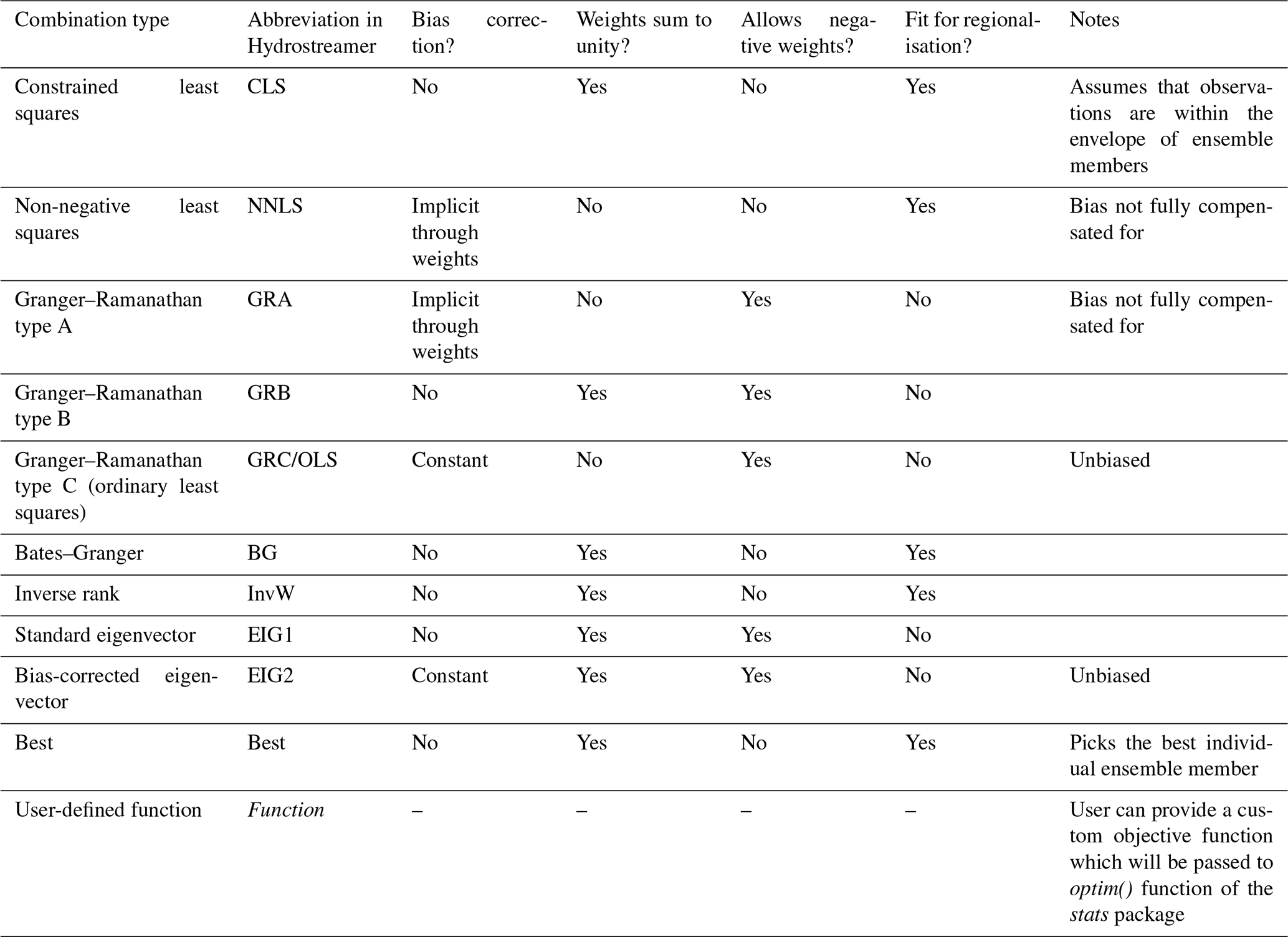
The third step in the typical Hydrostreamer workflow is model averaging. Model averaging using varying sizes of ensembles is a common approach to data assimilation in hydrological sciences (see e.g. Arsenault et al., 2015; Arsenault and Brissette, 2016; Gosling et al., 2010; Skøien et al., 2016; Velázquez et al., 2011; Zaherpour et al., 2019). In model averaging, an ensemble of time series is combined into a multi-model combination (MMC), commonly using a weighted approach. Provided that streamflow records are available, Hydrostreamer provides facilities for at-location model averaging, as well as regionalised model averaging. Table 1 provides an overview of all the implemented model averaging methods in Hydrostreamer along with some of their properties. The methods are based on minimising error between observations and the weighted ensemble average.
In a regionalisation experiment Arsenault and Brissette (2016) explore MMC weights using a small three-member ensemble, finding that MMCs are nearly always outperformed by the best-performing individual model member at regionalised locations and that a simple ensemble mean (each ensemble member receiving equal weights) performs reasonably well across all locations. They further conclude that regionalising model averaging weights is not a reasonable task; however their conclusions are based on a limited analysis of three methods which all allow negative weights. We argue that their conclusion applies to methods that allow for negative weights due to the fact that relationships between hydrological time series at different locations likely differ considerably. The lack of negative weights, we assume, is one reason that the ensemble mean is able to outperform their selected model averaging methods.
To help extend model averaging to ungauged basins (that is, any river segment which does not contain a monitoring station), we must find a way to regionalise model averaging weights. In Hydrostreamer, we consider those methods which do not allow negative weights as fit for regionalisation. This ensures that, while the performance of regionalised MMC weights may be worse than the best individual ensemble member (which we cannot know in an ungauged basin), the output hydrological time series is ensured to be positive.
In practise, in Hydrostreamer regionalisation of MMC weights is done so that each river segment receives model averaging weights from the nearest downstream gauging station, and if there are no downstream gauging stations, the ensemble mean is used instead.
Table 1Multi-model combination options implemented in Hydrostreamer v1.0.
Here we describe the Hydrostreamer workflow in Sect. 3.1 together with auxiliary functionality, which help in making use of alternative data inputs and working with the output. Following that we describe the input and output data structures in Sect. 3.2.
3.1 Functions used in Hydrostreamer v1.0 workflow
The functions used in a typical workflow and data requirements in Hydrostreamer are shown in the flow diagram in Fig. 2. Due to the large number of optional arguments and functionality, the figure only shows minimum required inputs. Complete up-to-date documentation and default values can be found on the model documentation website at https://mkkallio.github.io/hydrostreamer/, last access: 5 May 2021, or using the internal R help() function. The documentation site also provides a vignette which gives further information on the workflow of Hydrostreamer in the form of a practical example.
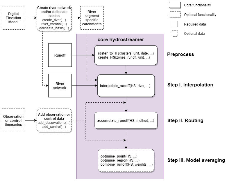
Figure 2Data requirements and related core workflow showing function names and minimal required input arguments. The steps refer to Fig. 1. The ellipsis marks optional function arguments.
The workflow starts from pre-processing data to a format with which Hydrostreamer is able to work. Hydrostreamer supports providing input hydrological variables either as raster or vector formats, each with dedicated functions, raster_to_HS() and create_HS(). Each raster cell or each polygon in the input data is considered a source zone. For the interpolation step, a network of target river lines and/or target zones need to be provided in addition to the HS object output from the pre-processing steps. The routing step requires the output from the interpolation step, the routing method (instantaneous, or constant velocity), and parameters for that routing method. Finally, model averaging can be performed (1) at the point location of the monitoring station, giving optimal time series for the monitoring station locations only; (2) regionally, where MMCs are provided for each river segment, optimised at the nearest downstream monitoring station, and (3) with user-provided combination weights.
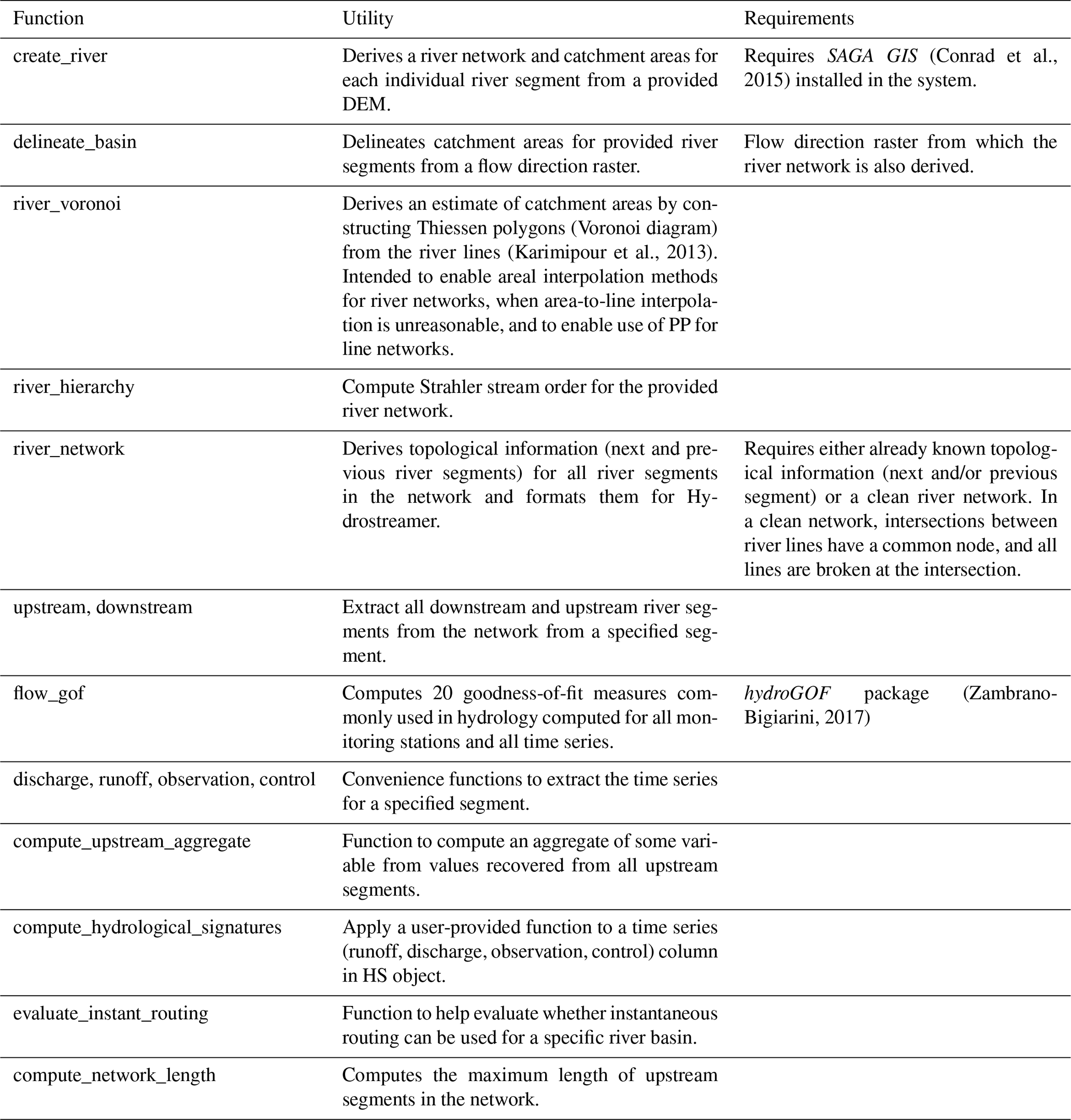
Once runoff data and the river network have been read into R, the full workflow can be achieved with only three to five chained commands, depending on whether the user wishes to apply model averaging. Hydrostreamer provides some additional functionality which supports the optional components in Fig. 2. These and further supporting functions are given in Table 2.
Table 2Auxiliary functions in Hydrostreamer v1.0, their intended utility, and their data and software requirements.
3.2 Data structures
The data structures used in Hydrostreamer are compatible with the packages from the tidyverse (Wickham et al., 2019) suite of packages, including chaining of commands with the pipe operator commonly associated with the tidyverse workflow. For spatial representation, R makes use of the simple features implementation for R (sf; Pebesma, 2018).
Hydrostreamer objects have class HS, which are essentially standard R data frames and which can be modified with any function that works on standard data frames. In a HS data.frame object, each row is either a source or target zone which is described by variables and time series in list columns. Each HS object contains at least a unique ID (riverID for target zones, or zoneID for source zones) and a time series column. Depending on the usage, the object can also have a number of other columns with variables such as topological network information (previous and next river segments) for the routing algorithms, names of monitoring stations, and various time series (e.g. runoff, discharge, control, observation time series) and variables which are used in the interpolation step. As the HS object is a data frame, additional columns with information the user wants to include can be added. For all the functions which add or modify HS specific columns, see Appendix A, Fig. A1.
Each time series is stored in a list column, where each element of the list is a data frame giving the time series for the target or source zone in question. Each of these tables is structured so that each row is a time step, for which the date is given by a column named “Date”. In runoff or discharge time series, each additional column is the estimate of an ensemble member. For control and observation time series, the table may contain only one column in addition to Date.
The river network structure follows a hierarchical node–link network, where each river segment is represented by a node which has links to previous and next river segments. This data model is simple and intuitive. Demir and Szczepanek (2017) find that this type of river network representation is generally more performant in different types of queries than alternative network representations. The adjacency information is stored in HS as list columns NEXT and PREVIOUS, which store all the river segment IDs which flow into the segment in question and which segments are topologically immediately downstream from it.
We conducted a case study in the Sesan, Sekong, and Srepok basins (3S from now on) in Southeast Asia to demonstrate Hydrostreamer functionality. The 3S basins are major transboundary tributaries of the Mekong River, located in Laos, Cambodia, and Vietnam. The area is influenced by the southwest monsoon, leading to distinct dry and wet seasons. The area is characterised by poor data coverage. We performed downscaling of 15 off-the-shelf global runoff products obtained from the ISIMIP 2a experiment (Gosling et al., 2017), providing an example use case where the scale (downscaling) and zonation (downscaling to non-conforming target units) effect are addressed with Hydrostreamer. We compared the performance of downscaled and routed discharge against the streamflow records in 10 hydrological stations obtained from the Mekong River Commission (MRC, 2017) and against the performance of two free and open global streamflow benchmark datasets. The data record extends from 1985 to 2008, with variable periods at each station. The following sub-sections detail the data used, performance measurement, and three conducted experiments, each building upon the previous one.
4.1 Data and pre-processing
The experiments build on three main data sources and two distributed global discharge estimates as benchmarks. First, we used the aforementioned ISIMIP 2a data archive (accessed in August 2018). We obtained all total runoff (variable “mrro” in the ISIMIP archive) and discharge (“dis”) time series, modelled with the variable social forcing (“varsoc”) scenario, available in the archive in monthly time steps. When monthly data products were not available, we used the daily product and aggregated it to monthly averages. The obtained datasets are summarised in Table 3. We did not use the products forced with the WATCH dataset, as it only extends until the end of 2001 and would have meant discarding some of our observation stations with records only after 2001. In total, we obtained products from 10 global hydrological models and land-surface models from the archive (from now on, both referred to as GHM). From the total of 24 runoff products, we only use those which also provided discharge output (n=15). The ISIMIP outputs are delivered with a spatial resolution of 0.5∘ (approximately 55 km at the Equator).
Table 3ISIMIP 2a total runoff and discharge datasets obtained from the ISIMIP data repository.
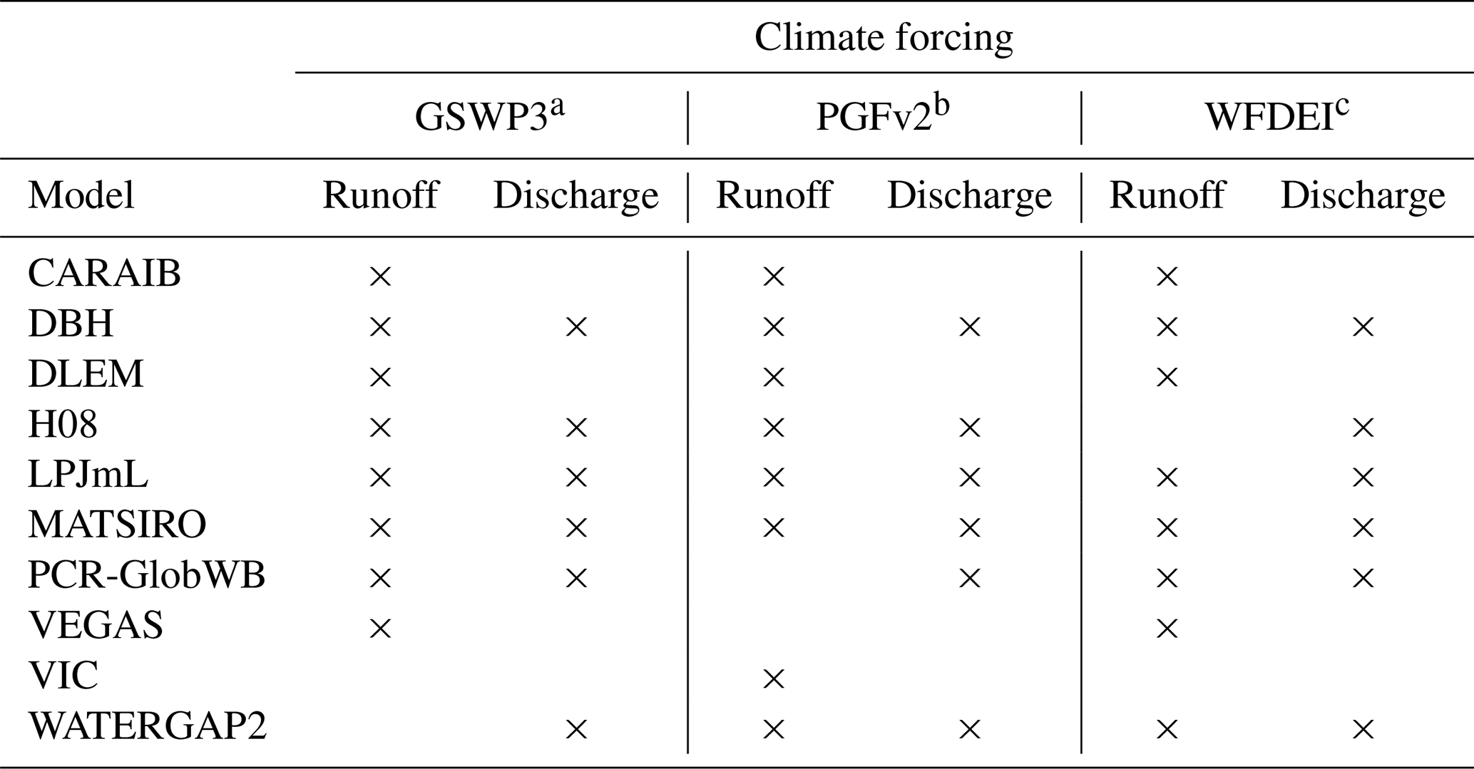
a Global Soil Wetness Project Phase 3, http://hydro.iis.u-tokyo.ac.jp/GSWP3/ (last access: 15 January 2021). b Updated version of Sheffield et al. (2006). c WATCH Forcing Data – ERA-Interim (Weedon et al., 2014).
The runoff time series were downscaled to the HydroSHEDS 30 arcsec resolution river network for Asia (Lehner and Grill, 2013). The total size of the river network within the 3S was 2115 river segments with a median length of 5055 m. To accommodate the evaluation of areal interpolation techniques, we also obtained the HydroSHEDS 30 arcsec resolution flow direction raster from which the river network was derived. We likewise obtained the HydroSHEDS DEM in order to derive an ancillary variable (see Sect. 4.3).
Similarly to the runoff and discharge GHM time series, the daily observed streamflow for the 10 MRC hydrological stations was aggregated to monthly by taking the mean monthly streamflow. For comparison, we additionally use two recent global streamflow products: GRADES (Global Reach-Level A Priori Discharge Estimates for SWOT; Lin et al., 2019) and GLOFAS reanalysis streamflow dataset (GLObal Flood Awareness System; Alfieri et al., 2020). GRADES is provided in zones similar to the HydroSHEDS river network product, albeit derived from a higher-resolution DEM. GLOFAS comes as a global grid with 0.1∘ resolution (∼11 km at the Equator). Both datasets are provided with a daily time step and were also aggregated to monthly means.
Figure 1a shows the 3S basin and the used HydroSHEDS dataset overlaid on the 0.5∘ model grid used in the ISIMIP data. The figure additionally shows the locations of the monitoring stations and the basins they drain from.
4.2 Performance measurement
We assessed the performance of the Hydrostreamer streamflow predictions and all benchmark datasets to the observation time series using commonly used metrics:
-
root-mean-square error (RMSE), a commonly used model performance metric (in principle, all model averaging techniques in Hydrostreamer minimise RMSE);
-
percent bias (PBIAS), used to estimate model bias in relative terms: mean error standardised to mean observed discharge;
-
Nash–Sutcliffe efficiency (NSE; Nash and Sutcliffe, 1970), a commonly used performance metric using mean observed streamflow as a benchmark;
-
coefficient of determination (R2), a standard measure of correlation of dynamics;
-
Kling–Gupta efficiency (KGE; Gupta et al., 2009), a multi-objective metric composed of mean error, variability, and dynamics.
4.3 Experiments
We conducted three experiments building upon one another. In the first experiment, we performed downscaling of the total runoff inputs using AWI (for DEM-delineated catchment areas, as well as Voronoi diagram-based delineation), DM (DEM-derived catchments with an ancillary dasymetric variable), and area-to-line interpolation (without dasymetric variable). As a dasymetric variable, we used a recently developed topographic index DUNE (Dissipation along unit length; Loritz et al., 2019) that is capable of distinguishing different runoff formation regimes and is computed from the HydroSHEDS DEM. We used instantaneous routing for this experiment, because the flow timing error M (Eq. 9) was found to be insignificant considering other potential sources of error (0.028 for the most upstream location and 0.004 for the 3S basin on average). The most representative river segment was selected from the HydroSHEDS network for each monitoring station location based on comparison to the location on an actual river network. For assessment of global model performance, we likewise selected the grid cell which best represents the monitoring station in the low-resolution DDM30 river network (Döll and Lehner, 2002) used in the ISIMIP framework. We expected that the downscaled Hydrostreamer time series should perform at least as well as, or better than, the discharge time series from the GHMs due to better representation of the drainage basins associated with each monitoring station.
In the second experiment, we performed model averaging at the monitoring stations and assessed how the uncertainty related to the model averaging weights affects performance of the optimised MMC. In particular, we use the constrained least squares (CLS) technique (Diks and Vrugt, 2010). CLS is constrained to positive weights only, and the sum of weights must equal 1 – this means that the MMC time series will never have higher or lower discharge than any individual ensemble member. The combinations are performed multiple times with different training periods to assess the uncertainty in the model averaging weights. We used three sampling strategies (each available in Hydrostreamer) for the selection of the training period: (1) random selection of 50 % of all the time steps in the observation record (performed 100 times for all stations), (2) random selection of 50 % of calendar years in the observation record (performed 50 times for all stations), and (3) training combinations for each calendar month separately, with random 50 % of available time steps for each month (performed 50 times for all stations). The time steps in the observation record not included in the training period were used for model evaluation. We also created 10 000 random combinations with a multi-stage sampling technique, first randomising the n number of models to include, second picking n random models, and third randomising positive weights among the randomised model selection using uniform distribution, with weights summing to unity in order to have comparable constraint in the randomisation as we have in CLS.
Finally, in the third experiment, we regionalise the optimised MMC weights at each monitoring station and evaluate their performance at the other monitoring stations on the same river.
The results of each of the three experiments are explored and discussed in the following subsections.
5.1 Experiment 1: downscaling (interpolation, routing)
The four tested downscaling methods (see Sect. 4.3) show a negligible difference across all used performance metrics, when averaged over monitoring stations (see Appendix A, Table A1). Station-wise, there are very small differences in all stations except Sesan Upstream-East, where the largest differences in performance between downscaling methods are up to 0.40 for NSE and 0.10 for KGE, both when downscaling H08 forced with PGFv2. Across the entire 3S Basin, the difference between downscaling methods becomes smaller as the basin size increases. This is expected: with the chosen instantaneous routing method being the only difference in discharge that comes from the basin boundary, since all runoff from the middle of the basin instantly flows through the station. As the basin size increases, the proportion of runoff contribution from the catchments at the basin boundary becomes increasingly small and thus is shown in decreasing difference in performance metrics. This is in line with Cunha et al. (2012), who find that in ensemble modelling uncertainty gets smaller with increasing basin size. Because the differences between the downscaling are so small apart from the Sesan Upstream-East station, we opt to continue the analysis on the simplest downscaling method: area-to-line interpolation. It should be noted, however, that Virkki (2019) showed that area-to-line interpolation causes larger uncertainties in the reach level than approaches using reach-specific catchment areas. Furthermore, Kallio et al. (2019) found in a study that included 126 catchments with natural flow regime that DM using DUNE as an ancillary variable does improve the performance of downscaling in topographically varying terrain.
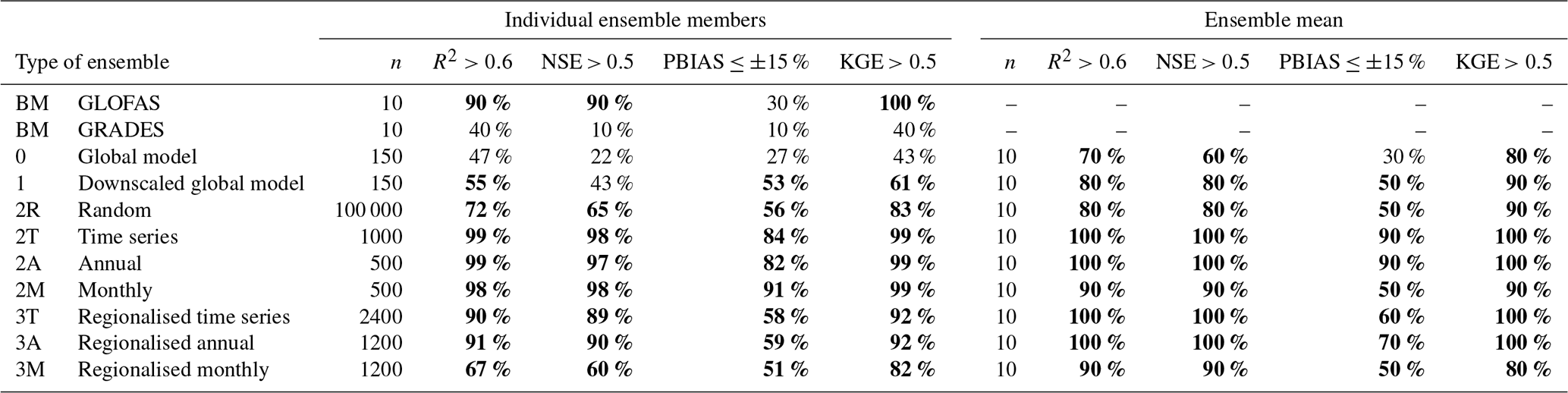
The performance of individual downscaled GHMs varies much more than the performance between tested downscaling methods (see Appendix A, Tables A2–A4). Compared to the discharge output from GHMs, the downscaled ones are similar or better in their performance, as seen in Fig. 3. Moriasi et al. (2015) recommend that for watershed scale models at monthly temporal resolution acceptable model performance is R2>0.60, NSE >0.50, and PBIAS %. Using these criteria, we find that they are fulfilled in 47 % and 55 % (R2), 22 % and 43 % (NSE), and 27 % and 53 % (PBIAS) of cases in downscaled GHMs and GHMs, respectively (see Table 4). Volume-wise the downscaled estimates fare better with mean (across all 15 GHM–climate forcing pairs, and all monitoring stations) PBIAS of −0.3 % against GHM's 11.2 %. The difference and direction in performance are visualised in Fig. 4, confirming our expectation that downscaling does improve the performance of GHM outputs.

Figure 3Comparison of Kling–Gupta efficiency compared to observed streamflow from the MRC for global model output and three experiments. Global model output: discharge from ISIMIP GHMs at 0.5∘ resolution (n=15), with results from benchmark products. Experiment 1: downscaled ISIMIP runoff. Experiment 2: multi-model combination (MMC) derived from random combinations and the three sampling strategies for CLS (i.e. constrained least squares; see Table 1) model averaging (2T, 2A, 2M). Experiment 3: using regionalised MMC weights derived in Experiment 2 at the gauges in the same river (Sekong, Sesan, or Srepok). KGE is shown for the testing period for Experiments 2 and 3 and for the entire time series for GHM discharge and Experiment 1.
Table 4Proportion of test cases (separate predictions at each station) satisfying performance criteria from Moriasi et al. (2015) for discharge and downscaled runoff from GHMs and for the different combination strategies tested. KGE is added to the criteria as an alternative to NSE and to allow comparison to Fig. 3. Values are shown for the test period for 2T, 2A, and 2M and for the entire time series for everything else. Proportions >50 % are shown in bold. BM stands for benchmark dataset.
Comparing to the openly available benchmark products GRADES and GLOFAS, the downscaled GHMs fare reasonably well. While the individual ensemble members have large spread in their performance, often being worse than either of the benchmarks, the ensemble mean provides consistent good performance with KGE >0.5 at all stations except Srepok Downstream (Fig. 3). The ensemble mean is considerably better performing than GRADES, at all stations but Srepok Downstream and Midstream. GLOFAS performs better than the ensemble mean at 6 of the 10 stations.
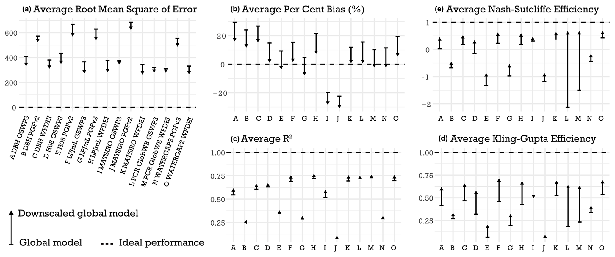
Figure 4Comparison of the performance of GHMs and downscaled GHMs averaged over all 10 monitoring stations.
5.2 Experiment 2: multi-model combinations at point locations
In the second experiment we performed model averaging on the 15-member ensemble with three combination strategies. For all stations, the time series and annual combination strategies produce very similar distribution in performance (Fig. 3, distributions 2T and 2A). Monthly combination (Fig. 3, distribution 2M) strategy can, however, produce better performance at point locations for PBIAS, which is lower than the threshold (PBIAS <15 %) in 91 % of all combinations (Table 4). However, when taking an ensemble mean from the 50 monthly combinations for each station, PBIAS threshold is satisfied in only half of the stations – and on the other hand the ensemble mean from time series or annual combinations performs considerably better. Comparing against the benchmarks, GRADES and GLOFAS, we see that all of the combination strategies can produce better performance (Fig. 3), with only a small minority of optimised MMC combinations showing worse performance for KGE.
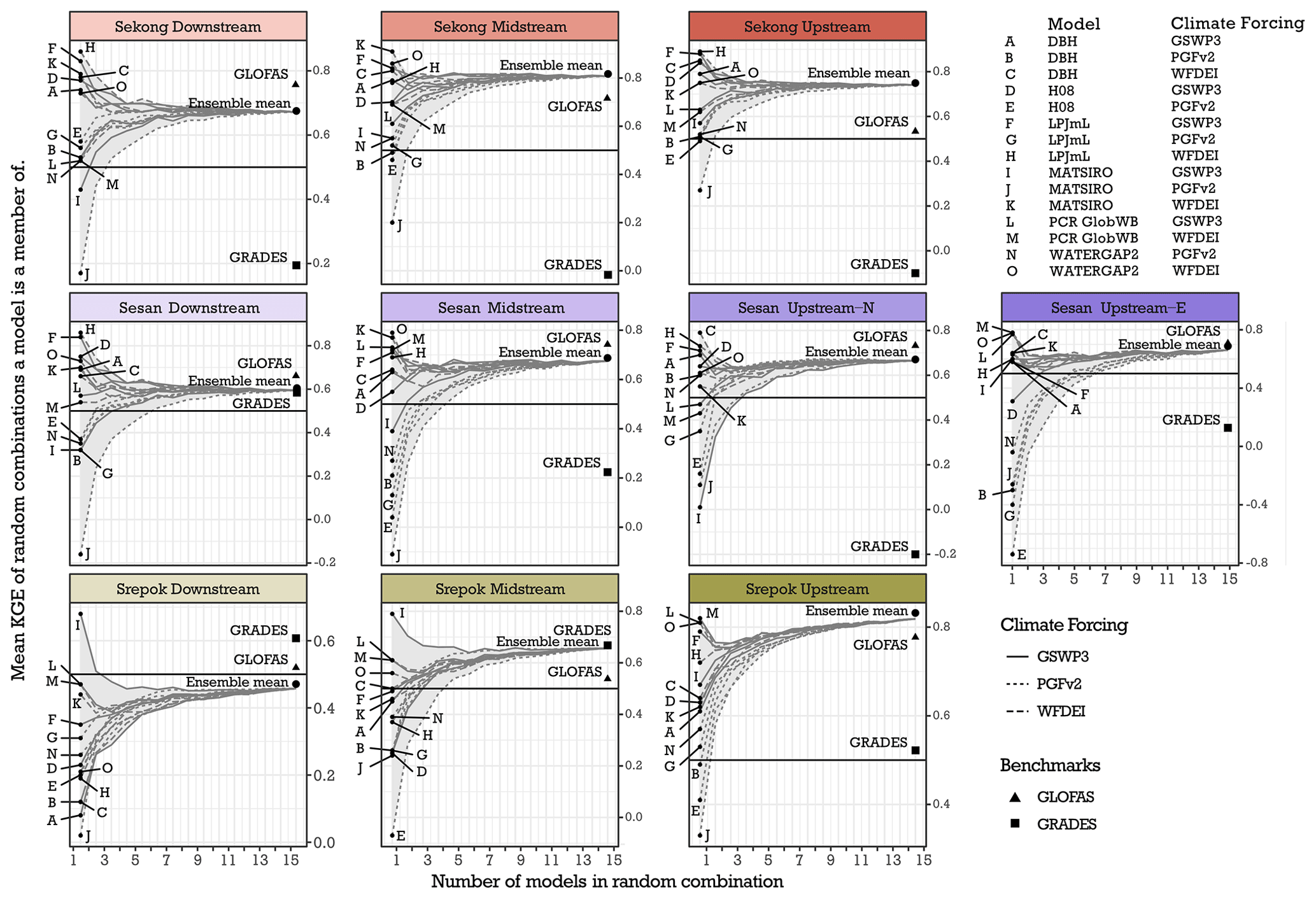
Figure 5KGE performance of individual downscaled runoff ensemble members and the mean KGE of the random ensembles each model is a member of. The two benchmarks GRADES and GLOFAS and the ensemble mean are marked for comparison.
When looking at individual ensemble members in Fig. 5, and their performance with random MMC weights, we see that the models have highly variable performance at different stations. The performance of individual ensemble members varies between stations (Fig. 5) and between indicators (Appendix A, Table A2). MATSIRO in particular shows high sensitivity to climate forcing; the performance when forced with PGFv2 has the largest mean RMSE, but forced with GSWP3 results in the smallest RMSE. In general, models forced with PGFv2 perform considerably worse at the 3S than when forced with WFDEI or GSWP3 (see Appendix A, Table A3).
The ensemble mean is robust throughout the basin; it is among the best performing individual members for most of the stations, and for Srepok Upstream it performs better than any single ensemble member. We can further infer from Fig. 5 that the skill of the ensemble mean stabilises at around 10–12 random ensemble members.
5.3 Experiment 3: regionalisation of multi-model combinations – prediction in ungauged basins
In the third experiment we tested the applicability of regionalising weights derived at one station to the other stations in the basin. We used weights derived from the stations with direct upstream or downstream linkage – Sekong, Sesan, and Srepok stations separately (refer to Fig. 1a). Our results suggest that the performance of regionalised model averaging weights is variable, as seen in Fig. 3. Regionalised time series and annual model averaging strategies produce commonly higher performance than the ensemble mean or the distribution of the random ensemble combinations, and in some stations can produce similar performance to the optimum for that station. This is desirable, as regionalisation of MMC weights would make no sense if the simple ensemble mean would perform better. We explored the distribution of weights at different stations and found that Sekong and Srepok stations produce an entirely different weighting of ensemble members. Sesan stations are somewhere between, with Sesan Downstream showing similar MMC weights to Sekong stations, and Sesan Upstream-East similar to Srepok River (the distribution of weights not shown). Sesan Midstream and Upstream-North appear unique in their sets of MMC weights. This is clearly seen in the distribution of performance of the Sesan stations in Fig. 3; there are clear clusters of performance from weights from the other stations, whereas Sekong and Srepok stations give a more uniform distribution in regionalised MMC performance.
The distribution of performance of the regionalised weights from monthly combinations is a clear case of overfitting – the distribution of performance (3M – the rightmost distribution in each facet in Fig. 3) is very large and is similar to or worse than the ensemble mean (Table 4). This is natural, since in the monthly weighting strategy we develop a set of 12 weights (one set for each month of the year) instead of a single set with time series and annual combination strategies. This suggests that monthly combinations are more useful for point optimisations but are not advantageous for use cases requiring regionalisation.
Hydrostreamer has been developed with two goals in mind: first, to support non-expert audiences in access to hydrological model data for their specific use cases and secondly to improve the usability of existing off-the-shelf hydrological products. Hydrostreamer can help non-experts in deriving hydrological variables they need by providing the means to avoid the pitfalls of hydrological modelling and to use data products prepared by experts. Hydrostreamer enables this by providing one way of dealing with MAUP (Goodchild and Lam, 1980) – the hydrological data product can be transformed to fit the analysis at hand. Using data products prepared and validated by experts can help in building confidence in the analysis results. With reference to the evaluation framework for environmental modelling developed by Hamilton et al. (2019), avoiding rushed modelling by inexperienced modellers can improve the confidence in several project-level elements of that framework – (1) efficiency by reducing time needed to produce estimates, (2) credibility by using outputs from professional hydrologists, (3) legitimacy by reducing bias when using multiple input runoff estimates, and (4) accessibility when using freely available runoff products.
The case study showed that overall, using global hydrological data products can produce results comparable to or better than openly available streamflow products with a global scope, even when the simplest possible case – area-to-line interpolation – is used. We attribute this to a better representation of the drainage network than in the 0.5∘ GHMs. Version 1.0 of Hydrostreamer has limitations, however, some of which we mention here. The biggest limitation of the current implementation is that DM and PP currently only allow temporally static weighting, similar to AWI. There are, however, many potential ancillary variables which may guide DM and PP which could be input with a time series. We plan that future versions of Hydrostreamer will support time series for the dasymetric and pycnophylactic variables, allowing dynamic interpolation.
The implemented instantaneous and constant flow velocity river routing methods are simpler than the commonly used methods (e.g. RAPID and MizuROUTE implement Muskingum and kinematic wave routing) but similar to a number of global hydrological models (Telteu et al., 2021). These two options are attractive due to their simplicity; the instantaneous routing solution does not have any parameters and the constant velocity has only one (flow velocity). The Muskingum–Cunge routing option may be more attractive for advanced users and when the simpler alternatives are not reasonable but comes at a cost of estimating Manning's roughness coefficient, bed slope, and river width. These may be estimated by the physical properties of the river segments, using a DEM, provided that such data are available. The routing solutions in Hydrostreamer do not, currently, include a reservoir or a lake model, which limits their applicability. Our case study area is devoid of large-scale dams during the simulation period, apart from Houay Ho and Yali built in 1999 and 2002, respectively. Models tend to be skilful in compensating for hydropower even when they are not represented in the models (as we can see from the high performance of MMC combinations at Sesan Midstream and Downstream stations located downstream from Yali). This, however, leads to overfitting and not a true representation of the parameters (Dang et al., 2020). In Hydrostreamer the relevant parameters are the MMC weights (if MA is applied) and any parameters required by the routing model. In our experimental results this is limited since Yali has been operational for only the last 6 years (out of a total of 23) of the streamflow record and influences only Sesan Midstream and Downstream stations. Houay Ho is located on a small tributary of Sekong and does not have a large influence on the flow regime. We plan to add simple reservoir and lake models into the routing methods; however, in Hydrostreamer v1.0 reservoirs can be represented through setting a boundary condition for the river segment in which a reservoir outlet is located.
The limitations in the model averaging step are most substantial in the regionalisation component. Hydrostreamer currently only supports regionalising weights to the upstream segments from a monitoring station up to the next monitoring station, defaulting to ensemble mean on every segment without a downstream dam. We plan to address this by adding further regionalisation options, for instance, based on proximity and similarity of river segments.
In this paper we presented Hydrostreamer v1.0, an R package designed to improve usability of hydrological data products and to support the use of hydrological data products by non-experts. Hydrostreamer does this particularly by addressing the modifiable area unit problem – pre-existing data products often arrive at a spatial aggregation or incompatible enumeration units which are not optimal for user analysis. This article includes an overview of the concepts and workflow Hydrostreamer is built upon: (areal) interpolation, routing, and model averaging. There are several features in Hydrostreamer which are not available in other software solutions in R: advanced areal interpolation method dasymetric mapping (for both area-to-area and area-to-line interpolation), pycnophylactic interpolation for polygon networks, and a combined pycnophylactic–dasymetric interpolation specifically designed for hydrological variables. Further, there are no other vector-based river routing solutions available for R. Hydrostreamer also facilitates data assimilation via model averaging when observation data are available.
To test the capabilities of Hydrostreamer, we performed a case study downscaling an ensemble of global runoff products onto a HydroSHEDS 15 arcsec river network. We show that an ensemble of coarse-resolution global hydrological products can be used to produce locally accurate streamflow time series – even with the simplest forms of areal and area-to-line interpolation. This we attribute to addressing MAUP by better representation of the drainage network and catchment areas. We find that model averaging weights can be transferred to ungauged locations, but with some limitations such as non-negativity of the weights and sufficient similarity of catchments. This represents a clear future research topic. We further find that an ensemble mean of global hydrological models can produce an adequate estimate for streamflow, at least for monthly time steps.
Hydrostreamer fills a niche where streamflow data are needed quickly, but limited resources (skill, time, money, input data) are available to set up a new modelling exercise. Using Hydrostreamer, reasonable-quality streamflow estimates can be extracted from existing runoff products with the addition of only a river network and historical streamflow records for model averaging. Hydrostreamer v1.0 is open source and available under the MIT licence from GitHub: http://github.com/mkkallio/hydrostreamer/ (last access: 5 May 2021).
Table A1The mean goodness-of-fit measurements of the tested downscaling methods at each monitoring station, averaged across all GHM–climate forcing pairs. Ordered by KGE.
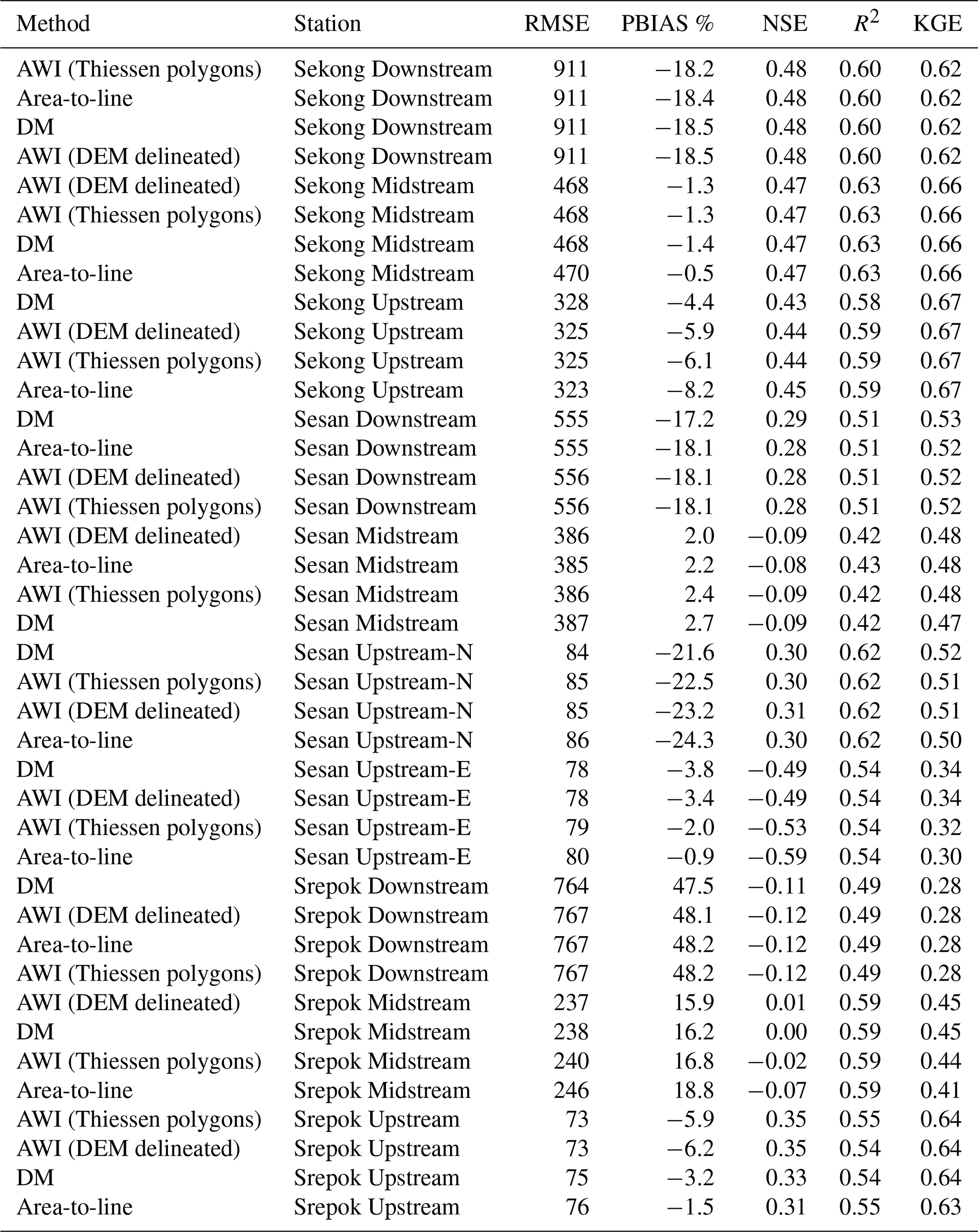
Table A2The mean goodness-of-fit measures of area-to-line downscaling method for all included GHM–climate forcing pairs. The values are averaged over all 10 monitoring stations.
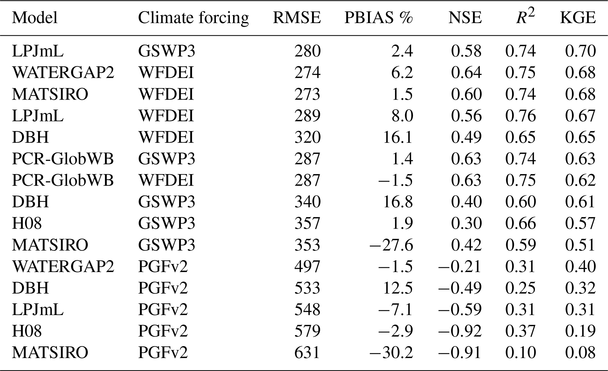
Table A3The mean performance of climate forcing datasets, averaged over all 10 monitoring stations and all GHMs.

Table A4The mean performance of GHMs, averaged over all climate forcing datasets and all 10 monitoring stations. It should be noted that PCR-GlobWB does not include a version forced with PGFv2, which in this basin has the highest error.
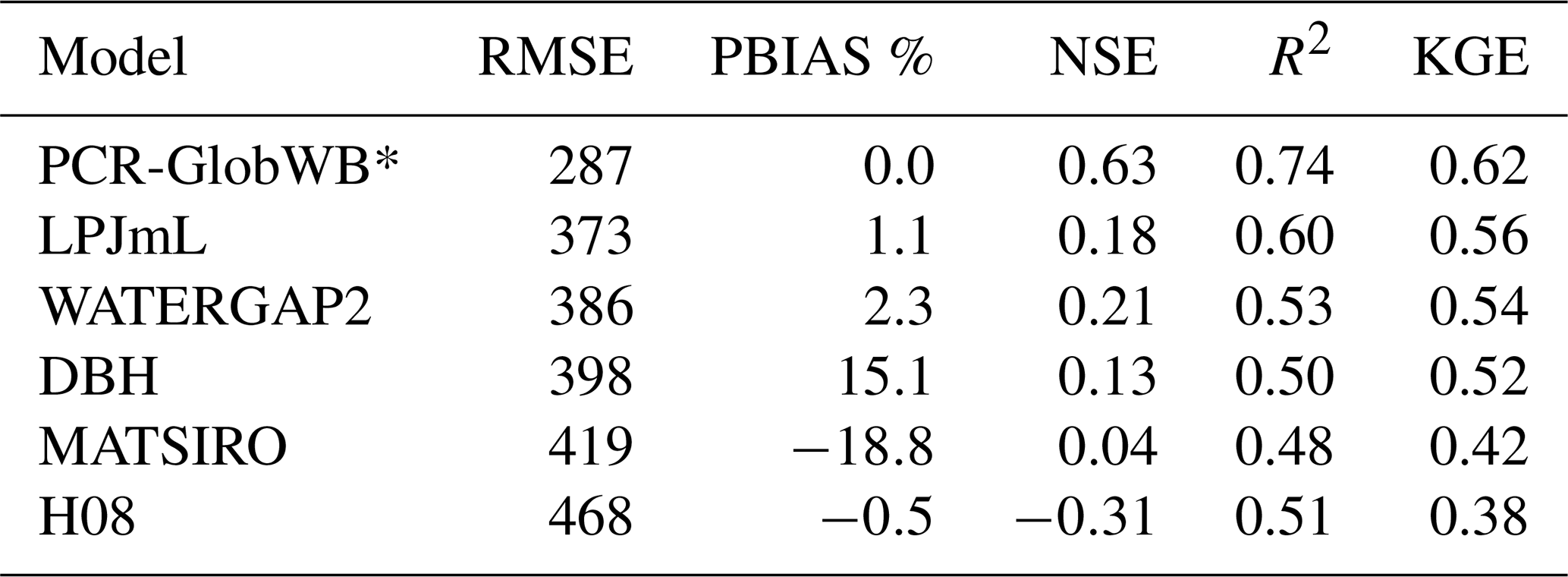
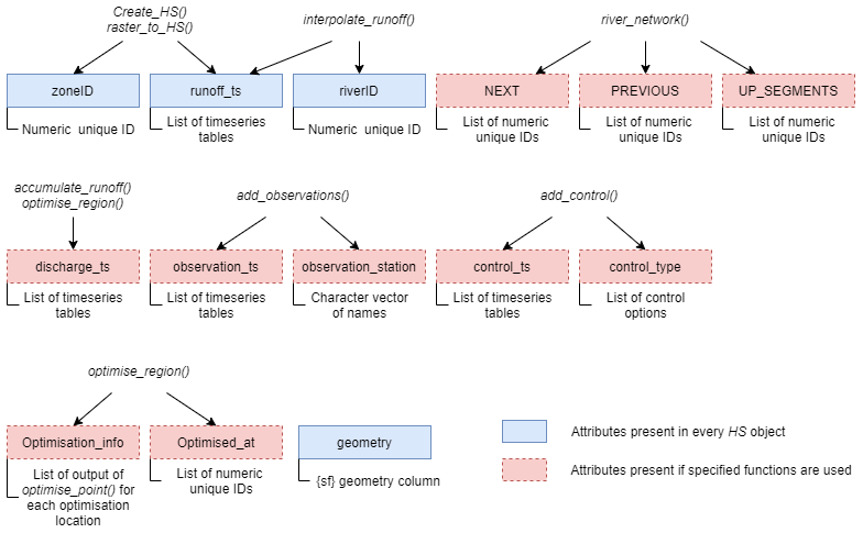
Figure A1Attribute columns which may be added by Hydrostreamer functions to an HS object and the functions which include them.
B1 Conceptual illustration of the constant flow velocity routing method implemented in Hydrostreamer v1.0
B2 Comparison of the three flow routing methods
The three streamflow routing methods were compared for our case study area using the LPJmL model forced with GSWP3 climate forcing. We ran the constant velocity routing with the default 1 m s−1 flow velocity. Muskingum–Cunge was run using a constant Manning's roughness coefficient of 0.03 and with a constant slope of 0.00025 for all river segments. For river width modelling, we used the power-law relationships between discharge and river width from Moody and Troutman (2002). Performance metrics used in the case study are shown in Table B1. The predicted time series are shown in Fig. B2. With the parameters given above, constant velocity routing performs the best. However, at a monthly timescale there is little practical difference between the methods in the study area. The performance of Muskingum–Cunge and constant velocity routing is expected to improve with optimised routing parameters and velocity.
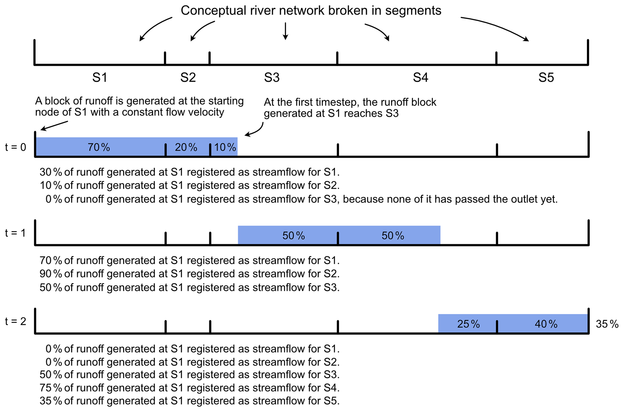
Figure B1Conceptual representation of the constant velocity algorithm, showing runoff produced at S1 at time step t=0 and how it is registered at downstream river segments.
Table B1Performance metrics of the three routing methods implemented in Hydrostreamer for the GHM LPJmL forced with GSWP3 climate dataset. MC stands for Muskingum–Cunge algorithm, Const. for constant velocity routing and Inst. for instantaneous routing.

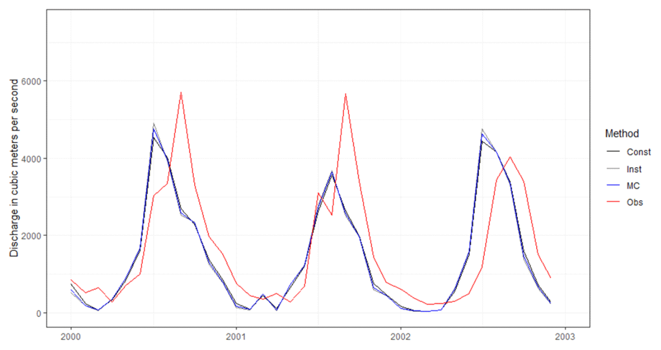
Figure B2Predicted monthly LPJmL-GSWP3 flow of the three routing methods at Sekong Downstream Station. Figure showing a sample of years 2000–2002. MC stands for Muskingum–Cunge algorithm, Const. for constant velocity routing, Inst. for instantaneous routing, and Obs. for observations.
The ISIMIP data used in this study are available from https://esg.pik-potsdam.de/search/isimip/ (last access: 5 May 2021). Benchmark dataset GRADES (Lin et al., 2019) is available for research purposes at http://hydrology.princeton.edu/data/mpan/MERIT_Basins/ (last access: 5 May 2021) and http://hydrology.princeton.edu/data/mpan/GRADES/ (15 January 2021), and GLOFAS (Alfieri et al., 2020) is available from https://cds.climate.copernicus.eu/cdsapp#!/dataset/cems-glofas-historical (last access: 15 January 2021). HydroSHEDS data are available from https://hydrosheds.org/ (last access: 15 January 2021). Streamflow data are available from the Mekong River Commission Data Portal at https://portal.mrcmekong.org/ (last access: 15 January 2021). Hydrostreamer v1.0.1 source code for this publication is deposited at https://doi.org/10.5281/zenodo.4739223 (Kallio and Virkki, 2021) with the latest version of the code hosted at GitHub: https://github.com/mkkallio/hydrostreamer (last access: 5 May 2021). Code and data (except for observed time series, due to license constraints) to reproduce the analysis and the output of downscaling and routing are archived at https://doi.org/10.5281/zenodo.4739212 (Kallio, 2020).
MKa planned and envisioned the software. MKa wrote the software with input from VV. MKa and JHAG designed the experiments. MKa wrote the manuscript with input from all the authors.
The authors declare that they have no conflict of interest.
Publisher's note: Copernicus Publications remains neutral with regard to jurisdictional claims in published maps and institutional affiliations.
We would like to thank the ISIMIP team and all participating modelling teams for making the outputs freely available.
Marko Kallio and Vili Virkki were funded by the Aalto University School of Engineering Doctoral Programme. Marko Kallio additionally received funding from Maa- ja Vesitekniikan Tuki ry. Matti Kummu received funding from the Academy of Finland project WATVUL (grant no. 317320), Emil Aaltonen Foundation project “eat-less-water”, and European Research Council (ERC) under the European Union's Horizon 2020 research and innovation programme (grant no. 819202) from which Vili Virkki received additional funding. Joseph H. A. Guillaume received funding from an Australian Research Council Discovery Early Career Researcher Award (project no. DE190100317).
This paper was edited by Richard Mills and reviewed by two anonymous referees.
Addor, N. and Melsen, L. A.: Legacy, Rather Than Adequacy, Drives the Selection of Hydrological Models, Water Resour. Res., 55, 378–390, https://doi.org/10.1029/2018WR022958, 2019.
Alfieri, L., Lorini, V., Hirpa, F. A., Harrigan, S., Zsoter, E., Prudhomme, C., and Salamon, P.: A global streamflow reanalysis for 1980–2018, J. Hydrol. X, 6, 100049, https://doi.org/10.1016/j.hydroa.2019.100049, 2020.
Allen, P. M., Arnold, J. C., and Byars, B. W.: Downstream Channel Geometry for Use in Planning-Level Models1, JAWRA J. Am. Water Resour. Assoc., 30, 663–671, https://doi.org/10.1111/j.1752-1688.1994.tb03321.x, 1994.
Arcement, G. J. and Schneider, V. R.: Guide for selecting Manning's roughness coefficients for natural channels and flood plains, Guide for selecting Manning's roughness coefficients for natural channels and flood plains, U.S. G.P.O., For sale by the Books and Open-File Reports Section, U.S. Geological Survey, https://doi.org/10.3133/wsp2339, 1989.
Arsenault, R. and Brissette, F.: Multi-model averaging for continuous streamflow prediction in ungauged basins, Hydrol. Sci. J., 61, 2443–2454, https://doi.org/10.1080/02626667.2015.1117088, 2016.
Arsenault, R., Gatien, P., Renaud, B., Brissette, F., and Martel, J.-L.: A comparative analysis of 9 multi-model averaging approaches in hydrological continuous streamflow simulation, J. Hydrol., 529, 754–767, https://doi.org/10.1016/j.jhydrol.2015.09.001, 2015.
Beven, K.: A manifesto for the equifinality thesis, J. Hydrol., 320, 18–36, https://doi.org/10.1016/j.jhydrol.2005.07.007, 2006.
Blair, P. and Buytaert, W.: Socio-hydrological modelling: a review asking “why, what and how?”, Hydrol. Earth Syst. Sci., 20, 443–478, https://doi.org/10.5194/hess-20-443-2016, 2016.
Brunner, M. I., Slater, L., Tallaksen, L. M., and Clark, M.: Challenges in modeling and predicting floods and droughts: A review, WIREs Water, 8, e1520, https://doi.org/10.1002/wat2.1520, 2021.
Brunsdon, C.: pycno: Pycnophylactic Interpolation, R package version 1.2, available at: https://CRAN.R-project.org/package=pycno (last access: 11 August 2021), 2014.
Chow, V. T.: Open-Channel Hydraulics, McGraw Hill, New York, 1959.
Comber, A. and Zeng, W.: Spatial interpolation using areal features: A review of methods and opportunities using new forms of data with coded illustrations, Geogr. Compass, 13, e12465, https://doi.org/10.1111/gec3.12465, 2019.
Conrad, O., Bechtel, B., Bock, M., Dietrich, H., Fischer, E., Gerlitz, L., Wehberg, J., Wichmann, V., and Böhner, J.: System for Automated Geoscientific Analyses (SAGA) v. 2.1.4, Geosci. Model Dev., 8, 1991–2007, https://doi.org/10.5194/gmd-8-1991-2015, 2015.
Cunge, J. A.: On The Subject Of A Flood Propagation Computation Method (Musklngum Method), J. Hydraul. Res., 7, 205–230, https://doi.org/10.1080/00221686909500264, 1969.
Cunha, L. K., Mandapaka, P. V., Krajewski, W. F., Mantilla, R., and Bradley, A. A.: Impact of radar-rainfall error structure on estimated flood magnitude across scales: An investigation based on a parsimonious distributed hydrological model, Water Resour. Res., 48, W10515, https://doi.org/10.1029/2012WR012138, 2012.
Dallaire, C. O., Lehner, B., Sayre, R., and Thieme, M.: A multidisciplinary framework to derive global river reach classifications at high spatial resolution, Environ. Res. Lett., 14, 024003, https://doi.org/10.1088/1748-9326/aad8e9, 2019.
Dang, T. D., Chowdhury, A. F. M. K., and Galelli, S.: On the representation of water reservoir storage and operations in large-scale hydrological models: implications on model parameterization and climate change impact assessments, Hydrol. Earth Syst. Sci., 24, 397–416, https://doi.org/10.5194/hess-24-397-2020, 2020.
Dark, S. J. and Bram, D.: The modifiable areal unit problem (MAUP) in physical geography, Prog. Phys. Geogr. Earth Environ., 31, 471–479, https://doi.org/10.1177/0309133307083294, 2007.
David, C. H., Maidment, D. R., Niu, G.-Y., Yang, Z.-L., Habets, F., and Eijkhout, V.: River Network Routing on the NHDPlus Dataset, J. Hydrometeorol., 12, 913–934, https://doi.org/10.1175/2011JHM1345.1, 2011.
Delaigue, O., Thirel, G., Coron, L., and Brigode, P.: airGR and airGRteaching: Two Open-Source Tools for Rainfall-Runoff Modeling and Teaching Hydrology, in: EPiC Series in Engineering, HIC 2018, 13th International Conference on Hydroinformatics, 541–548, https://doi.org/10.29007/qsqj, 2018.
Demir, I. and Szczepanek, R.: Optimization of river network representation data models for web-based systems, Earth Space Sci., 4, 336–347, https://doi.org/10.1002/2016EA000224, 2017.
Diks, C. G. H. and Vrugt, J. A.: Comparison of point forecast accuracy of model averaging methods in hydrologic applications, Stoch. Environ. Res. Risk Assess., 24, 809–820, https://doi.org/10.1007/s00477-010-0378-z, 2010.
Do, H. X., Gudmundsson, L., Leonard, M., and Westra, S.: The Global Streamflow Indices and Metadata Archive (GSIM) – Part 1: The production of a daily streamflow archive and metadata, Earth Syst. Sci. Data, 10, 765–785, https://doi.org/10.5194/essd-10-765-2018, 2018.
Döll, P. and Lehner, B.: Validation of a new global 30-min drainage direction map, J. Hydrol., 258, 214–231, https://doi.org/10.1016/S0022-1694(01)00565-0, 2002.
Eicher, C. L. and Brewer, C. A.: Dasymetric Mapping and Areal Interpolation: Implementation and Evaluation, Cartogr. Geogr. Inf. Sci., 28, 125–138, https://doi.org/10.1559/152304001782173727, 2001.
Eränen, D., Oksanen, J., Westerholm, J., and Sarjakoski, T.: A full graphics processing unit implementation of uncertainty-aware drainage basin delineation, Comput. Geosci., 73, 48–60, https://doi.org/10.1016/j.cageo.2014.08.012, 2014.
Ghiggi, G., Humphrey, V., Seneviratne, S. I., and Gudmundsson, L.: GRUN: an observation-based global gridded runoff dataset from 1902 to 2014, Earth Syst. Sci. Data, 11, 1655–1674, https://doi.org/10.5194/essd-11-1655-2019, 2019.
Goodchild, M. F. and Lam, N. S. N.: Areal interpolation: A variant of the traditional spatial problem, Geo-Process., 1, 297–312, 1980.
Goodchild, M. F., Anselin, L., and Deichmann, U.: A Framework for the Areal Interpolation of Socioeconomic Data, Environ. Plan. Econ. Space, 25, 383–397, https://doi.org/10.1068/a250383, 1993.
Gosling, S., Müller Schmied, H., Betts, R., Chang, J., Ciais, P., Dankers, R., Döll, P., Eisner, S., Flörke, M., Gerten, D., Grillakis, M., Hanasaki, N., Hagemann, S., Huang, M., Huang, Z., Jerez, S., Kim, H., Koutroulis, A., Leng, G., Liu, X., Masaki, Y., Montavez, P., Morfopoulos, C., Oki, T., Papadimitriou, L., Pokhrel, Y., Portmann, F. T., Orth, R., Ostberg, S., Satoh, Y., Seneviratne, S., Sommer, P., Stacke, T., Tang, Q., Tsanis, I., Wada, Y., Zhou, T., Büchner, M., Schewe, J., and Zhao, F.: ISIMIP2a Simulation Data from Water (global) Sector, GFZ Data Services, Potsdam, Germany, https://doi.org/10.5880/pik.2017.010, 2017.
Gosling, S. N., Bretherton, D., Haines, K., and Arnell, N. W.: Global hydrology modelling and uncertainty: running multiple ensembles with a campus grid, Philos. T. R. Soc. Math. Phys. Eng. Sci., 368, 4005–4021, https://doi.org/10.1098/rsta.2010.0164, 2010.
Gottschalk, L.: Interpolation of runoff applying objective methods, Stoch. Hydrol. Hydraul., 7, 269–281, https://doi.org/10.1007/BF01581615, 1993.
Gupta, H. V., Kling, H., Yilmaz, K. K., and Martinez, G. F.: Decomposition of the mean squared error and NSE performance criteria: Implications for improving hydrological modelling, J. Hydrol., 377, 80–91, https://doi.org/10.1016/J.JHYDROL.2009.08.003, 2009.
Hamilton, S. H., Fu, B., Guillaume, J. H. A., Badham, J., Elsawah, S., Gober, P., Hunt, R. J., Iwanaga, T., Jakeman, A. J., Ames, D. P., Curtis, A., Hill, M. C., Pierce, S. A., and Zare, F.: A framework for characterising and evaluating the effectiveness of environmental modelling, Environ. Model. Softw., 118, 83–98, https://doi.org/10.1016/j.envsoft.2019.04.008, 2019.
Hobeichi, S., Abramowitz, G., Evans, J., and Beck, H. E.: Linear Optimal Runoff Aggregate (LORA): a global gridded synthesis runoff product, Hydrol. Earth Syst. Sci., 23, 851–870, https://doi.org/10.5194/hess-23-851-2019, 2019.
Kallio, M.: mkkallio/GMD_hydrostreamer: GMD hydrostreamer manuscript code and part of the data (Version 1.0) [code], Zenodo, https://doi.org/10.5281/zenodo.4739212, 2020.
Kallio, M. and Virkki, V.: mkkallio/hydrostreamer: hydrostreamer v1.0.1 (Version 1.0.1) [code], Zenodo, https://doi.org/10.5281/zenodo.4739223, 2021.
Kallio, M., Virkki, V., Guillaume, J. H. A., and van Dijk, A. I. J. M.: Downscaling runoff products using areal interpolation: a combined pycnophylactic-dasymetric method, in: MODSIM2019, 23rd International Congress on Modelling and Simulation., 23rd International Congress on Modelling and Simulation (MODSIM2019), edited by: El Sawah, S., https://doi.org/10.36334/modsim.2019.K8.kallio, 2019.
Kar, B. and Hodgson, M. E.: A Process Oriented Areal Interpolation Technique: A Coastal County Example, Cartogr. Geogr. Inf. Sci., 39, 3–16, https://doi.org/10.1559/152304063913, 2012.
Karimipour, F., Ghandehari, M., and Ledoux, H.: Watershed delineation from the medial axis of river networks, Comput. Geosci., 59, 132–147, https://doi.org/10.1016/J.CAGEO.2013.06.004, 2013.
Krause, P., Boyle, D. P., and Bäse, F.: Comparison of different efficiency criteria for hydrological model assessment, Adv. Geosci., 5, 89–97, https://doi.org/10.5194/adgeo-5-89-2005, 2005.
Lehner, B. and Grill, G.: Global river hydrography and network routing: baseline data and new approaches to study the world's large river systems, Hydrol. Process., 27, 2171–2186, https://doi.org/10.1002/hyp.9740, 2013.
Lehner, B., Verdin, K., and Jarvis, A.: New Global Hydrography Derived From Spaceborne Elevation Data, Eos Trans. Am. Geophys. Union, 89, 93–94, https://doi.org/10.1029/2008EO100001, 2008.
Leopold, L. B. and Maddock Jr., T.: The hydraulic geometry of stream channels and some physiographic implications, The hydraulic geometry of stream channels and some physiographic implications, U.S. Government Printing Office, Washington, D.C., https://doi.org/10.3133/pp252, 1953.
Lin, P., Pan, M., Beck, H. E., Yang, Y., Yamazaki, D., Frasson, R., David, C. H., Durand, M., Pavelsky, T. M., Allen, G. H., Gleason, C. J., and Wood, E. F.: Global Reconstruction of Naturalized River Flows at 2.94 Million Reaches, Water Resour. Res., 55, 6499–6516, https://doi.org/10.1029/2019WR025287, 2019.
Lindsay, J. B. and Evans, M. G.: The influence of elevation error on the morphometrics of channel networks extracted from DEMs and the implications for hydrological modelling, Hydrol. Process., 22, 1588–1603, https://doi.org/10.1002/hyp.6728, 2008.
Linke, S., Lehner, B., Ouellet Dallaire, C., Ariwi, J., Grill, G., Anand, M., Beames, P., Burchard-Levine, V., Maxwell, S., Moidu, H., Tan, F., and Thieme, M.: Global hydro-environmental sub-basin and river reach characteristics at high spatial resolution, Sci. Data, 6, 283, https://doi.org/10.1038/s41597-019-0300-6, 2019.
Loritz, R., Kleidon, A., Jackisch, C., Westhoff, M., Ehret, U., Gupta, H., and Zehe, E.: A topographic index explaining hydrological similarity by accounting for the joint controls of runoff formation, Hydrol. Earth Syst. Sci., 23, 3807–3821, https://doi.org/10.5194/hess-23-3807-2019, 2019.
Manley, D.: Scale, Aggregation, and the Modifiable Areal Unit Problem, in: Handbook of Regional Science, edited by: Fischer, M. M. and Nijkamp, P., Springer Berlin Heidelberg, Berlin, Heidelberg, 1157–1171, https://doi.org/10.1007/978-3-642-23430-9_69, 2014.
Mizukami, N., Clark, M. P., Sampson, K., Nijssen, B., Mao, Y., McMillan, H., Viger, R. J., Markstrom, S. L., Hay, L. E., Woods, R., Arnold, J. R., and Brekke, L. D.: mizuRoute version 1: a river network routing tool for a continental domain water resources applications, Geosci. Model Dev., 9, 2223–2238, https://doi.org/10.5194/gmd-9-2223-2016, 2016.
Moody, J. A. and Troutman, B. M.: Characterization of the spatial variability of channel morphology, Earth Surf. Process. Landf., 27, 1251–1266, https://doi.org/10.1002/esp.403, 2002.
Moriasi, D. N., Gitau, M. W., Pai, N., and Daggupati, P.: Hydrologic and Water Quality Models: Performance Measures and Evaluation Criteria, Trans. ASABE, 58, 1763–1785, https://doi.org/10.13031/trans.58.10715, 2015.
MRC: MRC Data and Information Services Portal, available at: http://portal.mrcmekong.org/ (last access: 15 January 2021), 2017.
Nagle, N. N., Buttenfield, B. P., Leyk, S., and Speilman, S.: Dasymetric Modeling and Uncertainty, Ann. Assoc. Am. Geogr. Assoc. Am. Geogr., 104, 80–95, https://doi.org/10.1080/00045608.2013.843439, 2014.
Nash, J. E. and Sutcliffe, J. V.: River flow forecasting through conceptual models part I – A discussion of principles, J. Hydrol., 10, 282–290, https://doi.org/10.1016/0022-1694(70)90255-6, 1970.
Paiva, R. C. D., Durand, M. T., and Hossain, F.: Spatiotemporal interpolation of discharge across a river network by using synthetic SWOT satellite data, Water Resour. Res., 51, 430–449, https://doi.org/10.1002/2014WR015618, 2015.
Parajka, J., Merz, R., Skøien, J. O., and Viglione, A.: The role of station density for predicting daily runoff by top-kriging interpolation in Austria, J. Hydrol. Hydromech., 63, 228–234, https://doi.org/10.1515/johh-2015-0024, 2015.
Pebesma, E.: Simple Features for R: Standardized Support for Spatial Vector Data, The R Journal, 10, 439–446, 2018.
Ponce, V.: 10.6 Muskingum-Cunge Method, in: Fundamentals of Open Channel Hydraulics, San Diego State University, 2014.
Prener, C. and Revord, C.: areal: An R package for areal weighted interpolation, J. Open Source Softw., 4, 1221, https://doi.org/10.21105/joss.01221, 2019.
Rase, W.-D.: Volume-preserving interpolation of a smooth surface from polygon-related data, J. Geogr. Syst., 3, 199–213, https://doi.org/10.1007/PL00011475, 2001.
R Core Team: R: A Language and Environment for Statistical Computing, R Foundation for Statistical Computing, Vienna, Austria, 2019.
Salmivaara, A., Porkka, M., Kummu, M., Keskinen, M., Guillaume, J. H. A., and Varis, O.: Exploring the Modifiable Areal Unit Problem in Spatial Water Assessments: A Case of Water Shortage in Monsoon Asia, Water, 7, 898–917, https://doi.org/10.3390/w7030898, 2015.
Seibert, J. and Vis, M. J. P.: Teaching hydrological modeling with a user-friendly catchment-runoff-model software package, Hydrol. Earth Syst. Sci., 16, 3315–3325, https://doi.org/10.5194/hess-16-3315-2012, 2012.
Shaw, S. B., Beslity, J. O., and Colvin, M. E.: Working Toward a More Holistic Set of Hydrologic Principles to Teach Non-Hydrologists: Five Simple Concepts Within Catchment Hydrology, Hydrol. Process., 13485, https://doi.org/10.1002/hyp.13485, 2019.
Sheffield, J., Goteti, G., and Wood, E. F.: Development of a 50-Year High-Resolution Global Dataset of Meteorological Forcings for Land Surface Modeling, J. Climate, 19, 3088–3111, https://doi.org/10.1175/JCLI3790.1, 2006.
Singh, V. P. and Woolhiser, D. A.: Mathematical Modeling of Watershed Hydrology, J. Hydrol. Eng., 7, 270–292, https://doi.org/10.1061/(ASCE)1084-0699(2002)7:4(270), 2002.
Skøien, J. O., Merz, R., and Blöschl, G.: Top-kriging – geostatistics on stream networks, Hydrol. Earth Syst. Sci., 10, 277–287, https://doi.org/10.5194/hess-10-277-2006, 2006.
Skøien, J. O., Bogner, K., Salamon, P., Smith, P., and Pappenberger, F.: Regionalization of post-processed ensemble runoff forecasts, Proc. IAHS, 373, 109–114, https://doi.org/10.5194/piahs-373-109-2016, 2016.
Slater, L. J., Thirel, G., Harrigan, S., Delaigue, O., Hurley, A., Khouakhi, A., Prosdocimi, I., Vitolo, C., and Smith, K.: Using R in hydrology: a review of recent developments and future directions, Hydrol. Earth Syst. Sci., 23, 2939–2963, https://doi.org/10.5194/hess-23-2939-2019, 2019.
Subramanya, K.: Engineering hydrology, McGraw Hill Education, New York, 2017.
Telteu, C.-E., Müller Schmied, H., Thiery, W., Leng, G., Burek, P., Liu, X., Boulange, J. E. S., Andersen, L. S., Grillakis, M., Gosling, S. N., Satoh, Y., Rakovec, O., Stacke, T., Chang, J., Wanders, N., Shah, H. L., Trautmann, T., Mao, G., Hanasaki, N., Koutroulis, A., Pokhrel, Y., Samaniego, L., Wada, Y., Mishra, V., Liu, J., Döll, P., Zhao, F., Gädeke, A., Rabin, S. S., and Herz, F.: Understanding each other's models: an introduction and a standard representation of 16 global water models to support intercomparison, improvement, and communication, Geosci. Model Dev., 14, 3843–3878, https://doi.org/10.5194/gmd-14-3843-2021, 2021.
Tobler, W. R.: Smooth Pycnophylactic Interpolation for Geographical Regions, J. Am. Stat. Assoc., 74, 519–530, https://doi.org/10.2307/2286968, 1979.
Vatankhah, A. R. and Easa, S. M.: Depth-independent kinematic wave parameters for trapezoidal and power-law channels, Ain Shams Eng. J., 4, 173–183, https://doi.org/10.1016/j.asej.2012.08.010, 2013.
Velázquez, J. A., Anctil, F., Ramos, M. H., and Perrin, C.: Can a multi-model approach improve hydrological ensemble forecasting? A study on 29 French catchments using 16 hydrological model structures, Adv. Geosci., 29, 33–42, https://doi.org/10.5194/adgeo-29-33-2011, 2011.
Venhuizen, G. J., Hut, R., Albers, C., Stoof, C. R., and Smeets, I.: Flooded by jargon: how the interpretation of water-related terms differs between hydrology experts and the general audience, Hydrol. Earth Syst. Sci., 23, 393–403, https://doi.org/10.5194/hess-23-393-2019, 2019.
Virkki, V.: The value of open-source river streamflow estimation in Southeast Asia, available at: https://aaltodoc.aalto.fi/handle/123456789/36357 (last access: 1 January 2020), 2019.
Vrugt, J. A. and Robinson, B. A.: Treatment of uncertainty using ensemble methods: Comparison of sequential data assimilation and Bayesian model averaging, Water Resour. Res., 43, W01411, https://doi.org/10.1029/2005WR004838, 2007.
Weedon, G. P., Balsamo, G., Bellouin, N., Gomes, S., Best, M. J., and Viterbo, P.: The WFDEI meteorological forcing data set: WATCH Forcing Data methodology applied to ERA-Interim reanalysis data, Water Resour. Res., 50, 7505–7514, https://doi.org/10.1002/2014WR015638, 2014.
Wickham H., Averick M., Bryan J., Chang W., D’Agostino McGowan L., François R., Grolemund G., Hayes A., Henry L., Hester J., Kuhn M., Pedersen T. L., Miller E., Bache S. M., Müller K., Ooms J., Robinson D., Seidel D. P., Spinu V., Takahashi K., Vaughan D., Wilke C., Woo K., Yutani H.: Welcome to the Tidyverse, J. Open Source Softw., 4, 1686, https://doi.org/10.21105/joss.01686, 2019.
Wright, J. K.: A Method of Mapping Densities of Population: With Cape Cod as an Example, Geogr. Rev., 26, 103–110, https://doi.org/10.2307/209467, 1936.
Zaherpour, J., Mount, N., Gosling, S. N., Dankers, R., Eisner, S., Gerten, D., Liu, X., Masaki, Y., Müller Schmied, H., Tang, Q., and Wada, Y.: Exploring the value of machine learning for weighted multi-model combination of an ensemble of global hydrological models, Environ. Model. Softw., 114, 112–128, https://doi.org/10.1016/j.envsoft.2019.01.003, 2019.
Zambrano-Bigiarini, M.: hydroGOF: Goodness-of-fit functions for comparison of simulated and observed hydrological time series, Zenodo, https://doi.org/10.5281/zenodo.840087, 2017.
- Abstract
- Introduction
- Core Hydrostreamer v1.0 functionality
- Hydrostreamer v1.0 software architecture
- Case study method
- Case study results and discussion
- Planned future developments
- Conclusion
- Appendix A
- Appendix B
- Code and data availability
- Author contributions
- Competing interests
- Disclaimer
- Acknowledgements
- Financial support
- Review statement
- References