the Creative Commons Attribution 4.0 License.
the Creative Commons Attribution 4.0 License.
 | 17 Aug 2021
An iterative process for efficient optimisation of parameters in geoscientific models: a demonstration using the Parallel Ice Sheet Model (PISM) version 0.7.3
Steven J. Phipps
Jason L. Roberts
Matt A. King
Physical processes within geoscientific models are sometimes described by simplified schemes known as parameterisations. The values of the parameters within these schemes can be poorly constrained by theory or observation. Uncertainty in the parameter values translates into uncertainty in the outputs of the models. Proper quantification of the uncertainty in model predictions therefore requires a systematic approach for sampling parameter space. In this study, we develop a simple and efficient approach to identify regions of multi-dimensional parameter space that are consistent with observations. Using the Parallel Ice Sheet Model to simulate the present-day state of the Antarctic Ice Sheet, we find that co-dependencies between parameters preclude any simple identification of a single optimal set of parameter values. Approaches such as large ensemble modelling are therefore required in order to generate model predictions that incorporate proper quantification of the uncertainty arising from the parameterisation of physical processes.
- Article
(3815 KB) - Full-text XML
-
Supplement
(9498 KB) - BibTeX
- EndNote


The aim of any geoscientific model is typically to replicate the state and behaviour of real-world systems as accurately as possible, or at least with sufficient accuracy to generate useful insights into the problem being studied. This requires the model to incorporate a sufficiently accurate description of the real world, as well as sufficiently accurate data to provide boundary conditions and an initial state. However, geoscientific modelling inevitably involves making compromises in model design and implementation. Observational data, which is typically used to provide both initial and boundary conditions and to evaluate the models, can also be limited in accuracy and spatial coverage. Model error can therefore result from a number of sources, including missing or incomplete physics, missing or incomplete boundary conditions, and missing or incomplete initial conditions. This study focuses upon the first of these three potential sources of error, aiming to explore the contribution to model prediction error that arises from the simplifications made in the representation of physical processes within geoscientific models.
Either through choice or through necessity, physical processes are sometimes described by simplified schemes known as parameterisations (e.g. Hourdin et al., 2017). The values of the parameters within these schemes are often poorly constrained by theory or observation. Uncertainty in the parameter values translates into uncertainty in the outputs of the models. This uncertainty must be properly quantified in order to properly quantify the uncertainty in model predictions.
There are a number of reasons why parameterisations are required, or why a decision might be made to use them. These reasons include the following:
-
Lack of physical understanding. If a process is insufficiently well understood to enable a complete physical description, then it will need to be described in simplified terms.
-
Computational constraints. Models can be computationally expensive, in terms of the number of processors required to run the model, the amount of memory required to run the model and also in terms of the amount of time required to complete a simulation. Computational costs are increased if the user wishes to employ large ensemble modelling approaches (for example, to explore parameter space or to assess sensitivity to initial conditions). Even if a process is fully understood from a physical perspective, simplified parameterisations might therefore be required simply for reasons of computational feasibility.
-
Design choice. An intentional decision might be made to employ a parameterisation for the purposes of a process study.
The use of parameterisations rests upon a number of prior assumptions. These assumptions are usually made implicitly, rather than being stated explicitly. Key assumptions include the following:
-
That the underlying process can be adequately described by a parameterisation. The underlying model must be capable of replicating the real world, at least to a desired degree of accuracy. A parameterisation must therefore be capable of adequately describing the process that it seeks to replicate.
-
That optimal (true) parameter values exist. Optimal parameter values can only exist if the underlying model is capable of adequately replicating the real world, not just for one particular state but for the full spectrum of physical states that the model is designed to explore.
-
That these optimal (true) parameter values can be located. Even if optimal parameter values do exist, a means must exist to actually find them. Parameter values can have a direct theoretical or observational basis; otherwise sufficient observational data must exist, both to drive the model and to allow the model simulations to be evaluated. The model must also have a stable reference state and it must be possible to locate this; one category of model for which this might not be true is coupled atmosphere–ocean general circulation models, which are prone to drift (e.g. Sen Gupta et al., 2012) and can potentially exhibit multiple stable states (e.g. Hawkins et al., 2011). Computational constraints might also be a factor: it must be feasible to run a sufficiently large number of simulations, and to run simulations of a sufficiently long duration, to allow for adequate exploration of parameter space.
Thus, even if optimal parameter values do exist, a number of factors can prevent them from being meaningfully located. These factors include the availability of computational resources, which might constrain ensemble sizes and/or render it infeasible to integrate the model to a stable, equilibrium state, and the lack of sufficient, or sufficiently reliable, observational data to drive and evaluate the model. Interaction with other, possibly incomplete, parameterisations, or with finite model resolution and numerics, might also lead to the determination of incorrect parameter values. This might arise through cancellation of errors or through other more general error propagation mechanisms, such as the addition of errors or the selection of alternative branches through the model code. Finally, there are human constraints too: there may simply be too many interacting parameters for it to be feasible to perform any comprehensive parameter optimisation exercise within a realistic timeframe.
In practice, because of the time and effort required for parameter optimisation, the typical approach is simply to rely on prior published values. This can be the case even if these values were derived using a different version of the model or a different model configuration (for example, a different model resolution). This approach has the potential to result in inappropriate parameter choices, with the potential to introduce bias into model experiments. Using fixed parameter values in model ensembles will also mean that any uncertainties derived in the model predictions will not incorporate the contribution arising from the uncertainty in parameter values. This neglection of parameter uncertainty will result in an underestimation of the uncertainty in the model predictions.
Despite the challenges involved, there is an increasing emphasis on quantifying uncertainty in geoscientific modelling. This is apparent, for example, within the reports of the Intergovernmental Panel on Climate Change (e.g. Stocker et al., 2013). We therefore contend that, despite the challenges involved, parameter optimisation and sampling of parameter uncertainty should be a routine part of the process of geoscientific modelling. These efforts should also be documented as part of the process of publishing scientific results (e.g. Pittard, 2016).
The process of parameter optimisation is commonly referred to as “tuning” (e.g. Hourdin et al., 2017). Broadly speaking, the process of tuning a model typically involves integrating it to an equilibrium state under given boundary conditions (which are usually derived from observations, if suitable observations exist). The simulations are then evaluated against observational datasets, with the degree of model disagreement being quantified using a pre-defined cost function. Given knowledge of the evolution of a system over time, for example if information is available on past climate states, this process can be generalised to evaluate the ability of a model to simulate multiple different states (e.g. Forest et al., 2008). A model of the Antarctic Ice Sheet, for example, might be evaluated for its ability to simulate past warm or cold intervals (e.g. DeConto and Pollard, 2016).
The techniques used to optimise geoscientific models can be grouped into four broad categories:
-
Trial and error. This is the simplest technique and consists simply of running the model forwards multiple times, with different combinations of parameter values. The parameters can be varied separately (single-parameter optimisation) or simultaneously (multiple-parameter optimisation). Single-parameter approaches are simpler and more common (e.g. Pittard, 2016). However, if interactions exist between the values of different parameters, then only multiple-parameter approaches are capable of finding the optimal state of the model. Nonetheless, multiple-parameter optimisation can require large ensemble sizes to be effective, particularly if a large number of parameters are being optimised (e.g. Järvinen et al., 2010; Gladstone et al., 2012; Pollard et al., 2016). The efficacy of multiple-parameter approaches is therefore potentially limited by the computational resources available. Solutions include the application of adaptive sampling algorithms (e.g. Solonen et al., 2012), particle-based approaches (e.g. Lee et al., 2020) or the construction of an emulator or metamodel (simple statistical models that seek to describe the behaviour of vastly more complex computational models, e.g. O'Hagan, 2006; Neelin et al., 2010; Bellprat et al., 2012; Lee et al., 2013; Chang et al., 2014; McNeall et al., 2016; Williamson et al., 2017; Edwards et al., 2019; Gilford et al., 2020).
-
Bayesian techniques. These are statistical techniques that seek to incorporate prior knowledge on plausible parameter values (e.g. Jackson et al., 2004; Rougier, 2007; Forest et al., 2008; Sexton et al., 2012). The application of Bayesian techniques requires knowledge of the prior distributions of the parameter values, which are frequently unknown and which may require a relatively large number of ensemble simulations even for relatively low-dimensional parameter space (Guillas et al., 2009).
-
Inversion. Inversion requires the derivative of the model to each key parameter, which is obtained either through re-formulation of the model (a so-called adjoint model) or via an approximation of the derivative using methods such as finite differencing (e.g. Errico, 1997; Forget et al., 2015; Lyu et al., 2018). Inversion has the advantage that it enables much larger parameter spaces to be explored. However, the resulting inversions may only be applicable for one very specific model state and may therefore under-predict the uncertainty in model projections. Examples of the application of inversion using ice sheet models include PISM (van Pelt et al., 2013; Habermann et al., 2013), ISSM (Larour et al., 2012) and SICOPOLIS (Heimbach and Bugnion, 2009).
-
Machine learning. Machine learning techniques aim to enumerate unspecified relationships between input and output datasets, without requiring any understanding of the underlying physical processes (e.g. DeVries et al., 2017; Kim and Nakata, 2018). This allows for the discovery and utilisation of previously unknown relationships but does raise questions regarding the applicability for states that lie outside the range spanned by the training datasets.
In this study, because of the potential limitations associated with the alternatives, we adopt the first of these four approaches (trial and error). We attempt to reduce the computational cost of multi-parameter optimisation by developing a simple and efficient iterative approach to identify regions of multi-dimensional parameter space that are consistent with observations. We then demonstrate the application of this technique by using the Parallel Ice Sheet Model to simulate the present-day state of the Antarctic Ice Sheet. The methods are described in Sect. 2, while the results are presented and discussed in Sect. 3. Finally, conclusions are presented in Sect. 4.
2.1 Optimisation process
The iterative parameter optimisation process that we develop in this study consists of five key steps:
-
Identify the parameters to be optimised.
-
Select the initial ranges for each parameter.
-
Construct and run a perturbed-physics ensemble.
-
Evaluate each member of the ensemble against observations and determine which regions of parameter space, if any, can be rejected.
-
Repeat steps 3 and 4 until the process has converged, i.e. until no further changes are made to the ranges of any of the parameters.
Steps 1 and 2 will be informed by existing knowledge of the model and of the system being simulated. This might include theory, observations, prior published work and even preliminary modelling experiments that involve exploring the behaviour of individual parameters.
To illustrate the application of this process using a real-world geoscientific model, we will now present a demonstration using the Parallel Ice Sheet Model to simulate the present-day state of the Antarctic Ice Sheet (AIS).
2.2 Modelling framework
In this study, we use version 0.7.3 of the Parallel Ice Sheet Model (PISM), a highly parallel, open-source model that is suitable for large ensemble modelling and the simulation of large-scale marine ice sheets. Computational efficiency is achieved by employing a hybrid stress balance model to calculate ice velocities. PISM is described and evaluated for Antarctica, by Winkelmann et al. (2011), Martin et al. (2011) and Albrecht et al. (2015).
The model is written in C with MPI used for distributed-memory parallelism. The Portable, Extensible Toolkit for Scientific Computation (PETSc; Balay et al., 1997, 2015) is used to solve the model equations. Time stepping is explicit and adaptive. PISM has more than 200 user-configurable parameters, with the values set via command-line options (Albrecht et al., 2015).
The following is an outline summary of the key model physics. Specific aspects that form the target of the parameter optimisation are discussed in further detail later in this section. This description also reflects the specific configuration of the model used in this study and may not therefore accurately describe the configurations used in other studies.
2.2.1 Grid
The model is configured to simulate the present-day state of the entire AIS, with a horizontal resolution of 15 km×15 km and 101 quadratically spaced vertical levels.
2.2.2 Ice dynamics and thermodynamics
The two prognostic model variables are ice temperature and ice thickness. A hybrid approach is used to calculate the stress balance within the ice sheet, with the ice velocity being calculated by the superposition of two shallow stress balance approximations (Winkelmann et al., 2011). The shallow ice approximation (SIA) describes planar flow by shear parallel to the surface, while the shallow shelf approximation (SSA) describes membrane-type flow of floating ice or grounded ice sliding over a weak base (MacAyeal, 1989; Weis et al., 1999; Schoof, 2006). The SIA and SSA are both shallow approximations based on the assumption of a small thickness-to-width ratio for the ice sheet and are more computationally efficient than higher-order full-Stokes models. The flow law, which describes the relationship between the applied stress and the resulting deformation or strain rate, is described by the isotropic, polythermal scheme of Paterson and Budd (1982), Lliboutry and Duval (1985) and Aschwanden et al. (2012). An energy-conserving enthalpy-based model is used to calculate the ice temperature (Aschwanden and Blatter, 2009; Aschwanden et al., 2012).
2.2.3 Subglacier
PISM assumes that the ice sheet rests on a layer of till (Clarke, 2005). A spatially and temporally variable basal yield stress is determined by modelling a saturated subglacial till (Schoof, 2006; Bueler and Brown, 2009). The till friction angle is determined heuristically as a function of bed elevation, based on the hypothesis that till with a marine history should be weaker than till without such a history (Winkelmann et al., 2011; Martin et al., 2011; Aschwanden et al., 2013). A pseudo-plastic power law model is used to calculate the basal shear stress, and therefore to determine where sliding occurs. The subglacial hydrology model calculates the effective thickness of the layer of liquid water in the till, which is used to compute the effective pressure on the till, on a purely local basis (Tulaczyk et al., 2000; Bueler and Brown, 2009). No model of glacial isostatic adjustment is used in this study, as it is restricted to equilibrium simulations of the present-day state of the ice sheet.
2.2.4 Marine ice sheets
The lateral boundaries of the ice sheet are free to evolve (Winkelmann et al., 2011). Subgrid parameterisations are used to describe the positions of the ice shelf calving fronts (Albrecht et al., 2011) and the grounding lines (Gladstone et al., 2010; Feldmann et al., 2014). Calving is described using the physically based two-dimensional parameterisation of Levermann et al. (2012).
2.2.5 Boundary conditions
The topography follows Bedmap2 (Fretwell et al., 2013). Geothermal heat flow is taken from An et al. (2015). Climatological air temperature and precipitation for the period 1979–2014 are taken from the RACMO2.3 regional model (Van Wessem et al., 2014). The positive degree-day scheme of Calov and Greve (2005) is used to calculate the rate of surface melt. Following Pollard and DeConto (2012), Golledge et al. (2015) and DeConto and Pollard (2016), an atmospheric lapse rate correction of 8 K km−1 is used. The boundary-layer ocean model of Hellmer et al. (1998) and Holland and Jenkins (1999) is used to calculate the melt rate and temperature at the base of the floating ice shelves.
2.3 Step 1: Parameter selection
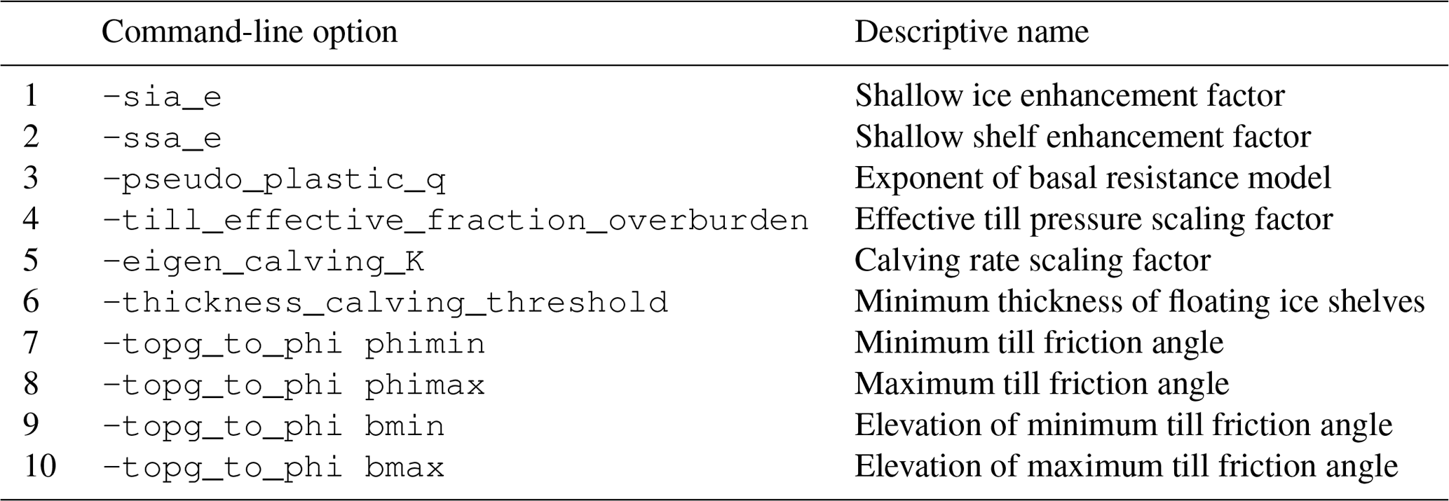
Through reading prior published work and the model documentation, 10 parameters are selected for optimisation on the basis that they describe key physical processes and that their values are not well constrained by either theory or observations. Out of the 10 parameters, 6 relate to the description of basal sliding, which is highly parameterised and involves parameters that are particularly poorly constrained (Albrecht et al., 2015). Two parameters relate to the description of the internal stress balance within the ice sheet, while the final two parameters relate to the description of calving. Table A1 provides the command-line options used by PISM to specify the values of each parameter, as well as a brief description. For ease of readability, the descriptive names provided in Table A1, rather than the names of the command-line options, will be used throughout this paper.
2.4 Step 2: Selection of initial ranges
The selection of initial parameter ranges is based on prior knowledge. PISM is distributed with a number of pre-configured experiments (Albrecht et al., 2015), with the configuration that forms the basis of this study being the Sea-level Response to Ice Sheet Evolution (SeaRISE; Bindschadler et al., 2013) experiment. The default parameter values specified for this experiment, as well as the values employed in previous studies that have used PISM to model the AIS, are provided in Table 1. These previous studies have modelled either the entire AIS or individual sectors and have used PISM to simulate the past, present and future states of the ice sheet:
-
Martin et al. (2011) simulate the present-day state of the AIS using a horizontal resolution of 19.98 km.
-
Golledge et al. (2015) simulate the present and future states of the AIS using horizontal resolutions of 20 and 10 km.
-
Pittard (2016) simulates the present and future states of the Lambert–Amery glacial system using a horizontal resolution of 5 km. Single-parameter perturbation experiments are used to select parameter values, with the ranges used for optimisation and the final values selected shown in Table 1.
-
Kingslake et al. (2018) simulate the evolution of the AIS over the past 205 000 years using a horizontal resolution of 15 km. An ensemble approach is used to sample uncertain parameters, with the ranges used for optimisation, and the final reference state selected, shown in Table 1.
Table 1The 10 physical parameters that are varied in this study: the default values for the pre-configured SeaRISE-Antarctica experiment in PISM and the values used in previous studies. M11: Martin et al. (2011). G15: Golledge et al. (2015). P16: Pittard (2016). K18: Kingslake et al. (2018). For G15, the values shown are those used at horizontal resolutions of 20 and 10 km, respectively. For P16 and K18, the values shown are the ranges used for parameter optimisation and the final values selected, respectively.
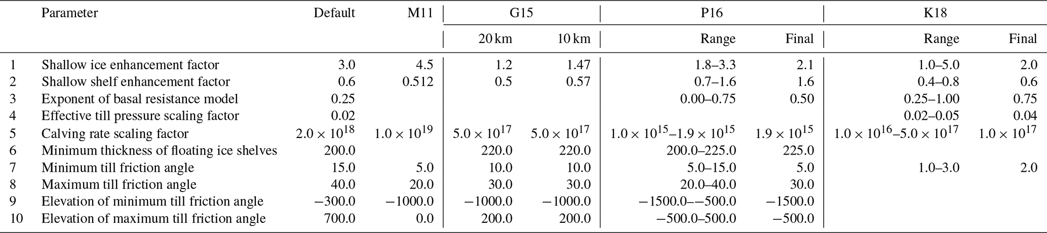
Shallow ice enhancement factor
The shallow ice enhancement factor is a flow enhancement factor for the non-sliding Shallow Ice Approximation, which is used to model grounded ice (Payne et al., 2000; Bueler et al., 2007). The factor sets the value of esia in Eq. (1), where Dij is the strain rate tensor, F is the function that describes the flow law, is the stress deviator tensor, T is the ice temperature, ω is the liquid water fraction, P is the pressure, and defines the second invariant σ of the stress deviator tensor (Albrecht et al., 2015).
Previous studies have used values of the shallow ice enhancement factor in the range 1.0–5.0 (Table 1). We therefore use this range as the initial range in this study.
Shallow shelf enhancement factor
The shallow shelf enhancement factor is a flow enhancement factor for the shallow shelf approximation (Weis et al., 1999). This approximation is used to model floating ice and is also used by PISM to describe ice streams and the sliding of grounded ice (Bueler and Brown, 2009). The enhancement factor sets the value of essa in Eq. (2), where ν is an effective viscosity, , and the other terms have the same meaning as in Eq. (1) (Albrecht et al., 2015).
Most previous studies have used values of the shallow shelf enhancement factor in the range 0.4–0.8; however, Pittard (2016) used values as large as 1.6 (Table 1). We use the full range 0.4–1.6 as the initial range in this study.
Exponent of basal resistance model
PISM uses a pseudo-plastic power law model to describe basal resistance (Albrecht et al., 2015). The exponent of the basal resistance model sets the value of q in Eq. (3), where τb is the basal shear stress, τc is the yield stress, u is velocity, and uthreshold is a parameter with a fixed value of 100 m a−1. Sliding occurs when the shear stress reaches the yield value.
Theoretically, the value of the exponent must lie in the range . Previous studies have used values that span the whole of this range. We therefore use the full range 0–1 as the initial range in this study.
Effective till pressure scaling factor
The yield stress τc in Eq. (3) is calculated as a function of a till friction angle ϕ and an effective till pressure Ntil (Albrecht et al., 2015).
The effective till pressure scaling factor sets the value of δ in Eq. (5), where Po is the ice overburden pressure, Wtil is the effective thickness of water in the till, and is the maximum amount of water in the till (Tulaczyk et al., 2000; Albrecht et al., 2015). The default values of e0=0.69 and Cc=0.12 are based on laboratory experiments (Tulaczyk et al., 2000).
We are only aware of one previous study that has varied the effective till pressure scaling factor parameter: Kingslake et al. (2018) explored values in the range 0.02–0.05, with a reference value of 0.04. We use the range 0.01–0.05 as the initial range in this study. This spans the published range of 0.02–0.05, but with a reduced lower bound of 0.01 chosen so that we sample values both above and below the default value in PISM of 0.02.
Calving rate scaling factor
PISM uses the calving scheme of Levermann et al. (2012). The calving rate scaling factor sets the value of K in Eq. (6), where c is the calving rate and and are the horizontal strain rates (Albrecht et al., 2015).
The units of c, K and are m s−1, m s and s−1, respectively. Levermann et al. (2012) find that values of K≳1×10⁹ m a [≳3.2×10¹⁶ m s] are required in order to maintain a stable grounding line, while a value of m a [ m s] is found to give the best agreement with observations. Previous studies have used values of the calving rate scaling factor in the range 1015–1019 m s (Table 1). We therefore use this range as the initial range in this study.
Minimum thickness of floating ice shelves
The calving scheme in PISM removes any ice at the calving front that is thinner than a specified minimum thickness (Albrecht et al., 2015).
Previous studies have used values in the range 200–225 m. However, observations suggest a wider plausible range of 150–250 m (Albrecht et al., 2015). We use this wider range as the initial range in this study.
Till friction angle parameters
PISM calculates the till friction angle ϕ in Eq. (4) as the function of four parameters (Albrecht et al., 2015).
Here, ϕmin and ϕmax are the minimum and maximum till friction angles, bmin and bmax are the elevations of the minimum and maximum till friction angles, b(x,y) is the bed elevation, and . By definition, ϕmin≤ϕmax and bmin≤bmax.
Previous studies have used values for ϕmin and ϕmax in the ranges 1–15∘ and 20–40∘, respectively. For ϕmin, we use the initial range 1–20∘ so that we include the full published range and sample values both above and below the default value in PISM of 15∘. For ϕmax, we use the initial range 20–40∘. Although this means that we do not sample values larger than the default value of 40∘, observations do not support values larger than this upper limit (Cuffey and Paterson, 2010).
Previous studies have used values for bmin and bmax in the ranges −1500 to −500 m and −500 to 500 m, respectively. For bmin, we use the published range −1500 to −500 m as the initial range in this study. While this range excludes the default value in PISM of −300 m, this is unavoidable given the constraint bmin≤bmax. For bmax, we use the initial range −500 to 1000 m. This includes the full published range and samples values both above and below the default value of 700 m.
2.5 Step 3: Ensemble construction and integration
A 100-member perturbed-physics ensemble is constructed. Each of the 10 parameters is perturbed independently, using a Latin hypercube approach (e.g. Helton and Davis, 2003) to sample the ranges of possible values. Latin hypercube sampling is employed here as, for a given ensemble size, it provides the most efficient representation of the variability spanned by the underlying parameter space. In the absence of any information on the distribution of prior probabilities, a uniform probability distribution is used for each parameter.
The specific set of parameter values used is generated using the lhs
function, which is part of the pyDOE package
(https://pythonhosted.org/pyDOE/, last access: 9 August 2021). Each member of the ensemble is
integrated to equilibrium under present-day boundary conditions, by employing
the following four-stage spin-up procedure:
-
The model is run for 1 year in bootstrapping mode (Albrecht et al., 2015) to initialise model fields. The initial geometry of the ice sheet is provided by Bedmap2 (Fretwell et al., 2013).
-
The model is run for 100 years, with basal sliding disabled, to smooth the surface of the ice sheet.
-
The model is run for 250 000 years, with fixed geometry (basal sliding and mass conservation disabled), in order to improve the enthalpy field.
-
Finally, the model is run for 100 000 years with full physics. This period is chosen to allow the simulated ice sheet to come into equilibrium with the boundary conditions, and thus to lose the memory of its initial state.
Stages 1–3 are fast and typically account for only ∼10 % of the total run time.
For this study, PISM is run on a Huawei E9000 cluster with each ensemble member using 224 cores. The queueing system for the cluster imposes a time limit of 48 h for each job, which is deemed to be sufficient as simulations typically take ∼6–12 h to complete. However, during each iteration, a small number of ensemble members can fail to complete. There are two reasons for this:
-
PISM uses an adaptive time-stepping scheme controlled by both the maximum diffusivity and the solutions to the mass conservation and energy conservation equations (Bueler et al., 2007; Bueler and Brown, 2009; Albrecht et al., 2015). This can result in large decreases in the time step (and hence large increases in the computational time required to complete a simulation) if numerical instabilities arise. The duration of the time step depends upon model resolution, the geometry of the ice sheet and the ice dynamics (and thus on the parameter choices). In a small number of cases involving extreme parameter values, ensemble members can therefore fail to complete within the time limit of 48 h.
-
Ensemble members can fail to complete the simulation because of numerical errors.
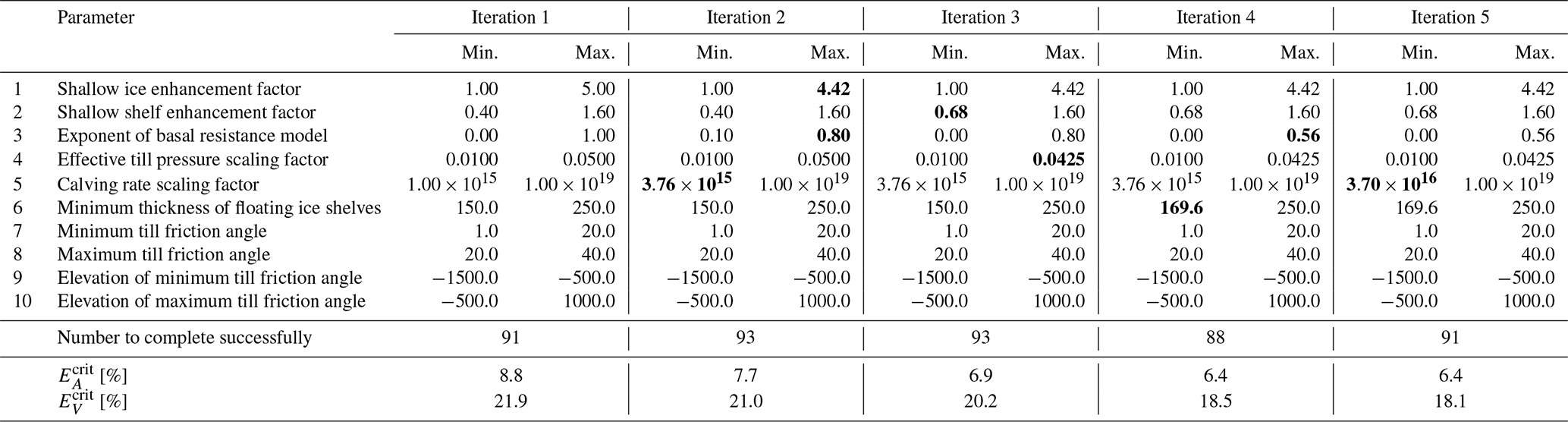
The total number of ensemble members to complete successfully for each iteration is shown in Table 2.
Table 2The convergence of the iterative parameter optimisation process for the 10 physical parameters varied in this study. For each iteration, the values shown are the minimum and maximum of the range sampled for that parameter. Bold text indicates a change in the value from the previous iteration. Also shown are the number of ensemble members to complete the simulation successfully during each iteration, as well as the critical values of the error metrics EA and EV.
2.6 Step 4: Model evaluation
Each ensemble member is evaluated to determine whether the simulated state of the AIS is realistic. Two error metrics are calculated, as follows.
EA measures the error in the two-dimensional geometry of the ice sheet and therefore measures errors in the location of the ice margin (including the calving fronts of the floating ice shelves). Mmod and Mobs are masks for the simulated and observed ice sheet, respectively, and are set equal to 1 where ice is present and 0 where it is not. EA is normalised by the observed area of the ice sheet Aobs and is then multiplied by 100 to convert it to a percentage. EA is equal to zero when the model is in perfect agreement with observations, with larger values representing increasing errors in the two-dimensional geometry of the simulated ice sheet. Equation (8) does not distinguish between grounded and floating ice.
EV measures the error in the three-dimensional geometry of the ice sheet and therefore measures errors in the simulated ice thickness. Hmod and Hobs are the simulated and observed ice thickness, respectively, with EV being normalised by the observed volume of the ice sheet Vobs and then multiplied by 100 to convert it to a percentage. EV is equal to zero when the model is in perfect agreement with observations, with larger values representing increasing errors in the three-dimensional geometry of the simulated ice sheet.
To determine whether each individual ensemble member can be considered to be “realistic”, it is necessary to define critical values of EA and EV. In the absence of any objective criterion that can be applied, the critical values are determined at each iteration of the parameter optimisation process by selecting the top tercile of ensemble members. Specifically, the critical value is determined by selecting the one-third of ensemble members with the smallest values of EA; similarly, the critical value is determined by selecting the one-third of ensemble members with the smallest values of EV. This allows the skill metrics to evolve during the parameter optimisation process, guided by the potential skill of the model being optimised. The values of and for each iteration are shown in Table 2.
To determine whether part of the range for each parameter can be rejected, it is necessary to perform a statistical test. For parameter X, let the range of values used to generate the ensemble be XA to XB. Let N members of the ensemble satisfy the criteria and and let the maximum value of X for these members be Xmax. Under the null hypothesis that all values of X in the range XA to XB are equally plausible, the probability that all N members will have X≤Xmax simply through random chance is given by
If the probability p is less than a pre-determined critical value pcrit, the null hypothesis can be rejected. In this case, XB is replaced with Xmax for the next iteration.
Similarly, if the minimum value of X for these N ensemble members is Xmin, the probability that all N members will have X≥Xmin simply through random chance is given by
If p is less than pcrit, the null hypothesis can be rejected and XA is replaced with Xmin for the next iteration.
The value of pcrit should be chosen carefully: if it is too large, there will be an excessive number of false positives, and regions of parameter space that are capable of generating skilful simulations will be rejected unnecessarily. However, if the value is too small, the iterative optimisation process will not be useful for refining the ranges for each parameter. We suggest therefore that the value of pcrit should be chosen such that the expected number of false positives at each iteration is no greater than 0.5. If n parameters are being optimised, then 2n significance tests will be performed at each iteration (one for the minimum value of each parameter, and one for the maximum value). In this case, the value of pcrit is given by
In this study n=10 and Eq. (12) therefore gives a value of pcrit=3.41 %.
2.7 Step 5: Convergence
Table 2 shows the progression of the iterative parameter optimisation process. Convergence is achieved after five iterations, at which point the statistical tests described by Eqs. (10) and (11) do not result in a rejection of the null hypothesis for any of the 10 parameters. No further changes are therefore made to either the minimum or maximum values for each parameter.
During the optimisation process, the ranges for all four of the parameters used to determine the till friction angle remain unchanged. However, for the other six parameters, the ranges are reduced in width by between 14.5 % (the shallow ice enhancement factor) and 44.0 % (the exponent of the basal resistance model). Overall, the volume of the parameter space has been reduced to just 14.6 % of the original size, meaning that 85.4 % of the possible parameter combinations have been eliminated. We note that the application of the technique described in this paper involves a trade-off between computational expense (as determined by the ensemble size) and precision (as measured by the reduction in parameter uncertainty). Increasing the ensemble size might allow a greater reduction in the volume of parameter space, but at the expense of increased computational cost.
The final ranges for two of the parameters are noteworthy within the context of previous work. We find that values of the shallow shelf enhancement factor smaller than 0.68 are not consistent with observations, or at least not for the specific version and specific configuration of the model used here. This excludes both the default value used by PISM (0.6) and the final values used in all previous studies with the exception of Pittard (2016). We also reject values of the calving rate scaling parameter smaller than 3.70×10¹⁶ m s, which is consistent with the finding of Levermann et al. (2012) that values ≳3.2×10¹⁶ m s are required to produce a stable grounding line.
For the final iteration of the optimisation process, 91 of the 100 ensemble members complete successfully (i.e. they do not fail because of numerical errors or because of exceeding the time limit). Of these members, by definition, one-third satisfy the criterion (Eq. 8) and one-third satisfy the criterion (Eq. 9). Only 14 of the original 100 ensemble members satisfy both of these criteria. This reflects the use of model-guided evaluation metrics during the optimisation process and does not mean that the other ensemble members are not useful. Nonetheless, we can examine these 14 members to gain insights into the performance of the model and the relationships between the model parameters.
The simulated ice thickness for each of the 14 ensemble members is shown in Fig. 1, while the errors relative to observations are shown in Fig. 2. The simulated states of the AIS are extremely similar, with all members having ice sheets that are too thick in coastal areas and along the Antarctic Peninsula. This suggests systematic errors arising either from the basic physics of the model or from the boundary conditions applied (for example, excessive precipitation). The simulated ice sheet is also generally too thin in inland areas, although it can be slightly too thick in some ensemble members (particularly ensemble members 63 and 83).
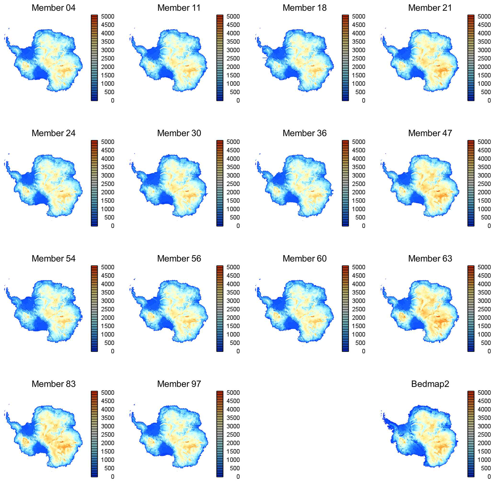
Figure 1The simulated ice thickness (m) for the 14 ensemble members that are in best agreement with observations. The observed ice thickness (Bedmap2; Fretwell et al., 2013) is also shown for comparison.
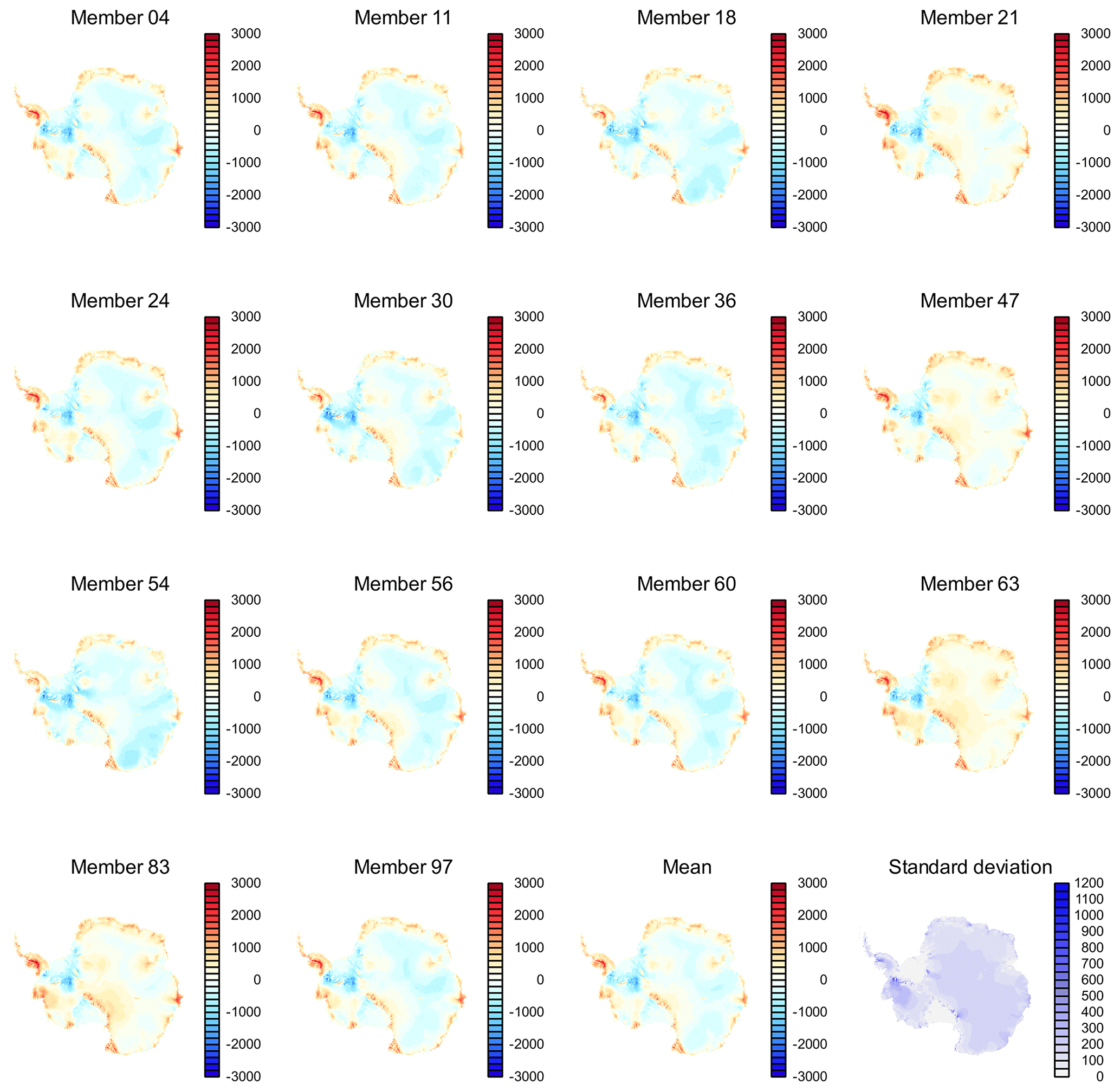
Figure 2The error in the simulated ice thickness (m) relative to Bedmap2 (Fretwell et al., 2013) for the 14 ensemble members that are in best agreement with observations. The ensemble mean and ensemble standard deviation of the error in the simulated ice thickness are also shown (bottom right).
Table 3The values of each physical parameter for the 14 ensemble members that are in best agreement with observations. For the name of each parameter, see Tables 1 and 2.

Table 4The Pearson correlation coefficients between each pair of the 10 physical parameters, for the 14 ensemble members that are in best agreement with observations. Bold text indicates that the correlation coefficient is statistically significant at the p=0.01 probability level. For the name of each parameter, see Tables 1 or 2.
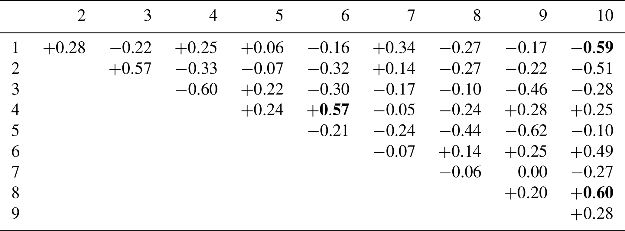
The parameter combinations used in each ensemble member, as well as the values of EA and EV, are shown in Table 3. For all 10 parameters, the values are distributed throughout the range. We can use these 14 sets of parameter values to determine the degree of covariance between parameters, within the set of model configurations that can be considered to be realistic. The Pearson correlation coefficient between each possible pair of parameters is shown in Table 4. Using bootstrapping to determine statistical significance, there are three pairs for which it is possible to reject the null hypothesis of no relationship at the p=0.01 probability level. These relationships are examined in Fig. 3.

Figure 3Scatter plots of the relationships between the three pairs of physical parameters identified in Table 4: (a) elevation of maximum till friction angle versus shallow ice enhancement factor; (b) minimum thickness of floating ice shelves versus effective till pressure scaling factor; and (c) elevation of maximum till friction angle versus maximum till friction angle. Values are shown for all 91 ensemble members that completed the final iteration successfully. The larger dots indicate the 14 ensemble members that are in best agreement with observations.
In each case, there are plausible physical explanations for the relationships:
-
Elevation of maximum till friction angle versus shallow ice enhancement factor. Increasing the elevation of the maximum till friction angle (bmax in Eq. 7) will tend to reduce the till friction angle ϕ and hence reduce the yield stress τc (Eq. 4). Reducing the shallow ice enhancement factor (e in Eq. 1) will tend to compensate for this by reducing ice flow, accounting for the negative relationship.
-
Minimum thickness of floating ice shelves versus effective till pressure scaling factor. Increasing the minimum thickness of the floating ice shelves will increase the calving rate and hence tend to result in an ice sheet with a smaller volume. Increasing the effective till pressure scaling factor (δ in Eq. 5) will tend to compensate for this by increasing the yield stress τc (Eq. 4) and hence reducing ice flow, accounting for the positive relationship.
-
Elevation of maximum till friction angle versus maximum till friction angle. Varying the elevation of the maximum till friction angle and the maximum till friction angle (bmax and ϕmax, respectively, in Eq. 7) together will leave the value of the till friction angle ϕ unchanged throughout most of the vertical range. This accounts for the positive relationship.
Nonetheless, the existence of such relationships indicates that there is no single configuration of the model that can be considered to be optimal, at least on the basis of the evaluation conducted in this study.
We have shown that the optimal ranges for each parameter can be dependent on other variables. While we have been able to substantially reduce the volume of plausible parameter space, limitations on our understanding of the underlying physical system ensure that the plausible ranges remain large for some parameters. Using additional observational and palaeoclimate datasets to evaluate the model, such as the surface ice velocity and vertical profiles of temperature and age from ice cores, might allow us to constrain the parameter ranges further.
Nonetheless, to sample equally from amongst all plausible model configurations requires the systematic sampling of parameter space. Different sampling strategies might be superior to others, with the application of these strategies (for example, the size of Latin hypercube ensembles) being potentially constrained by computational considerations. The size of the ensemble presented in this study (100) is relatively small, particularly given the large number of parameters being optimised (10). Chang et al. (2014) show that a 100-member Latin hypercube ensemble cannot adequately resolve the interactions between parameters in an ice sheet model, even when being used to study a five-dimensional parameter space. Ideally, our technique would therefore use a larger ensemble size or would be used to target a smaller number of model parameters. While the former would increase the computational cost, either of these modifications should allow for greater refinement of parameter ranges.
Fundamentally, however, the systematic sampling of parameter space requires the application of large ensemble modelling approaches. We also emphasise the importance of such modelling approaches when generating projections. Proper ensemble design is necessary not just to quantify uncertainty around the mean or median response of the system, but also to correctly identify the mean or median response itself. The importance of these points is demonstrated by DeConto and Pollard (2016) and Edwards et al. (2019), who find that parameter uncertainty and ensemble design influence the probability distributions for projections of future sea level rise. In particular, Edwards et al. (2019) emulate an ice sheet model and find that the probability distributions are skewed towards lower values; failure to take this into account might lead to overestimates of the most likely rate of sea level rise during the coming centuries.
Finally, we note that, whereas the approach developed in this study allows for the rigorous quantification of uncertainty in model parameters, and therefore the quantification of uncertainty in model projections, the technique presented here does not allow these uncertainty ranges to be interpreted in probabilistic terms. Extending our approach to generate future projections with associated probability distributions would require larger ensembles and further understanding of the uncertainties inherent in the physical system. This would include uncertainties in our physical understanding of that system, in the numerical representation of that physical understanding within the model and in the boundary conditions applied to the model.
We have developed a simple and efficient iterative technique for optimising parameters in geoscientific models. Specifically, our approach is able to eliminate regions of parameter space that are inconsistent with observations. While it is analogous to other techniques that use large ensemble modelling to refine parameter ranges (e.g. Solonen et al., 2012; Lee et al., 2020), the approach developed here is considerably simpler and should therefore be more accessible to the geoscientific modelling community.
We have demonstrated the application of our technique by using PISM to simulate the present-day state of the AIS. After five iterations, we were able to refine the ranges of 6 out of 10 parameters. Most significantly, we find that multiple different parameter combinations are able to generate equally skillful simulations. This suggests that, at least for the model and for the experiments used in this study, ice sheet models have no single optimal configuration and therefore cannot be meaningfully “tuned”. Using single model configurations to generate predictions is therefore likely to underestimate the magnitude of the uncertainty around the best estimates. The solution to this is to use large ensemble modelling approaches with perturbed parameters.
Given the existence of parameter uncertainty, exploring parameter space is essential. However, the behaviour of the model may depend upon the parameter values in non-trivial (and, in particular, non-linear) ways: this requires systematic exploration of parameter space. Identifying implausible regions of parameter space allows for more efficient exploration of those regions that are potentially consistent with observations.
Correct values for geoscientific model parameters may be unknown or may not even exist given that parameterisations by their very nature represent simplifications of real-world processes. The parameter uncertainties identified in this study, and in other studies that have used analogous large ensemble modelling approaches (e.g. Chang et al., 2014; Edwards et al., 2019; Gilford et al., 2020; Lee et al., 2020), represent a source of uncertainty in future climate projections. Further exploration of these uncertainties should form the basis of further work.
Table A1The 10 physical parameters that are varied in this study: the command-line option used by PISM and a descriptive name. The descriptive names are used throughout the paper.
All the source code and data associated with this study are deposited at Zenodo: https://doi.org/10.5281/zenodo.4275053 (Phipps et al., 2020). The specific version of the PISM manual referenced in this study (Albrecht et al., 2015) is also provided as Supplement.
The supplement related to this article is available online at: https://doi.org/10.5194/gmd-14-5107-2021-supplement.
SJP and JLR conceived the experiments. SJP conducted the experiments and analysed the output. All authors wrote the paper.
The authors declare that they have no conflict of interest.
This work was supported by the Centre for Southern Hemisphere Oceans Research, a joint research centre between the Qingdao National Laboratory for Marine Science and Technology (China) and the Commonwealth Scientific and Industrial Research Organisation (CSIRO; Australia). It was also supported by the University of Tasmania and the Australian Government's NCRIS program, through the Tasmanian Partnership for Advanced Computing. Development of PISM is supported by NSF grants PLR-1603799 and PLR-1644277 and NASA grant NNX17AG65G. The authors acknowledge use of the PyFerret program to generate the graphics in this paper. We thank Xuebin Zhang, two anonymous reviewers and the editor, Heiko Goelzer, for their comments, which have greatly improved the paper.
This research has been supported by the Australian Research Council (grant nos. SR140300001 and SR200100008).
This paper was edited by Heiko Goelzer and reviewed by two anonymous referees.
Albrecht, T., Martin, M., Haseloff, M., Winkelmann, R., and Levermann, A.: Parameterization for subgrid-scale motion of ice-shelf calving fronts, The Cryosphere, 5, 35–44, https://doi.org/10.5194/tc-5-35-2011, 2011. a
Albrecht, T., Aschwanden, A., Brown, J., Bueler, E., DellaGiustina, D., Feldman, J., Fischer, B., Habermann, M., Haseloff, M., Hock, R., Khroulev, C., Levermann, A., Lingle, C., Martin, M., Mengel, M., Maxwell, D., van Pelt, W., Seguinot, J., Winkelmann, R., and Ziemen, F.: PISM User's Manual, manual date 30 June 2015, based on PISM revision stable v0.7.1-2-g79b8840, 2015. a, b, c, d, e, f, g, h, i, j, k, l, m, n, o, p
An, M., Wiens, D. A., Zhao, Y., Feng, M., Nyblade, A., Kanao, M., Li, Y., Maggi, A., and Lévêque, J.: Temperature, lithosphere-asthenosphere boundary, and heat flux beneath the Antarctic Plate inferred from seismic velocities, J. Geophys. Res.-Sol. Ea., 120, 8720–8742, https://doi.org/10.1002/2015JB011917, 2015. a
Aschwanden, A. and Blatter, H.: Mathematical modeling and numerical simulation of polythermal glaciers, J. Geophys. Res., 114, F01027, https://doi.org/10.1029/2008JF001028, 2009. a
Aschwanden, A., Bueler, E., Khroulev, C., and Blatter, H.: An enthalpy formulation for glaciers and ice sheets, J. Glaciol., 58, 441–457, https://doi.org/10.3189/2012JoG11J088, 2012. a, b
Aschwanden, A., Aðalgeirsdóttir, G., and Khroulev, C.: Hindcasting to measure ice sheet model sensitivity to initial states, The Cryosphere, 7, 1083–1093, https://doi.org/10.5194/tc-7-1083-2013, 2013. a
Balay, S., Gropp, W. D., McInnes, L. C., and Smith, B. F.: Efficient Management of Parallelism in Object Oriented Numerical Software Libraries, in: Modern Software Tools in Scientific Computing, edited by: Arge, E., Bruaset, A. M., and Langtangen, H. P., Birkhäuser Press, Boston, Massachusetts, 163–202, 1997. a
Balay, S., Abhyankar, S., Adams, M. F., Brown, J., Brune, P., Buschelman, K., Dalcin, L., Eijkhout, V., Gropp, W. D., Kaushik, D., Knepley, M. G., McInnes, L. C., Rupp, K., Smith, B. F., Zampini, S., and Zhang, H.: PETSc Users Manual, Tech. Rep. ANL-95/11 – Revision 3.6, Argonne National Laboratory, Argonne, Illinois, 2015. a
Bellprat, O., Kotlarski, S., Lüthi, D., and Schär, C.: Objective calibration of regional climate models, J. Geophys. Res., 117, D23115, https://doi.org/10.1029/2012JD018262, 2012. a
Bindschadler, R. A., Nowicki, S., Abe-Ouchi, A., Aschwanden, A., Choi, H., Fastook, J., Granzow, G., Greve, R., Gutowski, G., Herzfeld, U., Jackson, C., Johnson, J., Khroulev, C., Levermann, A., Lipscomb, W. H., Martin, M. A., Morlighem, M., Parizek, B. R., Pollard, D., Price, S. F., Ren, D., Saito, F., Sato, T., Seddik, H., Seroussi, H., Takahashi, K., Walker, R., and Wang, W. L.: Ice-sheet model sensitivities to environmental forcing and their use in projecting future sea level (the SeaRISE project), J. Glaciol., 59, 195–224, https://doi.org/10.3189/2013JoG12J125, 2013. a
Bueler, E. and Brown, J.: Shallow shelf approximation as a ”sliding law” in a thermomechanically coupled ice sheet model, J. Geophys. Res., 114, F03008, https://doi.org/10.1029/2008JF001179, 2009. a, b, c, d
Bueler, E., Brown, J., and Lingle, C.: Exact solutions to the thermomechanically coupled shallow ice approximation: effective tools for verification, J. Glaciol., 53, 499–516, https://doi.org/10.3189/002214307783258396, 2007. a, b
Calov, R. and Greve, R.: A semi-analytical solution for the positive degree-day model with stochastic temperature variations, J. Glaciol., 51, 173–175, https://doi.org/10.3189/172756505781829601, 2005. a
Chang, W., Applegate, P. J., Haran, M., and Keller, K.: Probabilistic calibration of a Greenland Ice Sheet model using spatially resolved synthetic observations: toward projections of ice mass loss with uncertainties, Geosci. Model Dev., 7, 1933–1943, https://doi.org/10.5194/gmd-7-1933-2014, 2014. a, b, c
Clarke, G. K. C.: Subglacial processes, Annu. Rev. Earth Pl. Sc., 33, 247–276, https://doi.org/10.1146/annurev.earth.33.092203.122621, 2005. a
Cuffey, K. and Paterson, W. S. B.: The Physics of Glaciers, Academic Press, Burlington, Massachusetts, 4th edn., 2010. a
DeConto, R. M. and Pollard, D.: Contribution of Antarctica to past and future sea-level rise, Nature, 531, 591–597, https://doi.org/10.1038/nature17145, 2016. a, b, c
DeVries, P. M. R., Thompson, T. B., and Meade, B. J.: Enabling large-scale viscoelastic calculations via neural network acceleration, Geophys. Res. Lett., 44, 2662–2669, https://doi.org/10.1002/2017GL072716, 2017. a
Edwards, T. L., Brandon, M. A., Durand, G., Edwards, N. R., Golledge, N. R., Holden, P. B., Nias, I. J., Payne, A. J., Ritz, C., and Wernecke, A.: Revisiting Antarctic ice loss due to marine ice-cliff instability, Nature, 566, 58–64, https://doi.org/10.1038/s41586-019-0901-4, 2019. a, b, c, d
Errico, R. M.: What Is an Adjoint Model?, B. Am. Meteorol. Soc., 78, 2577–2592, 1997. a
Feldmann, J., Albrecht, T., Khroulev, C., Pattyn, F., and Levermann, A.: Resolution-dependent performance of grounding line motion in a shallow model compared with a full-Stokes model according to the MISMIP3d intercomparison, J. Glaciol., 60, 353–360, https://doi.org/10.3189/2014JoG13J093, 2014. a
Forest, C. E., Stone, P. H., and Sokolov, A. P.: Constraining climate model parameters from observed 20th century changes, Tellus, 60, 911–920, https://doi.org/10.1111/j.1600-0870.2008.00346.x, 2008. a, b
Forget, G., Campin, J.-M., Heimbach, P., Hill, C. N., Ponte, R. M., and Wunsch, C.: ECCO version 4: an integrated framework for non-linear inverse modeling and global ocean state estimation, Geosci. Model Dev., 8, 3071–3104, https://doi.org/10.5194/gmd-8-3071-2015, 2015. a
Fretwell, P., Pritchard, H. D., Vaughan, D. G., Bamber, J. L., Barrand, N. E., Bell, R., Bianchi, C., Bingham, R. G., Blankenship, D. D., Casassa, G., Catania, G., Callens, D., Conway, H., Cook, A. J., Corr, H. F. J., Damaske, D., Damm, V., Ferraccioli, F., Forsberg, R., Fujita, S., Gim, Y., Gogineni, P., Griggs, J. A., Hindmarsh, R. C. A., Holmlund, P., Holt, J. W., Jacobel, R. W., Jenkins, A., Jokat, W., Jordan, T., King, E. C., Kohler, J., Krabill, W., Riger-Kusk, M., Langley, K. A., Leitchenkov, G., Leuschen, C., Luyendyk, B. P., Matsuoka, K., Mouginot, J., Nitsche, F. O., Nogi, Y., Nost, O. A., Popov, S. V., Rignot, E., Rippin, D. M., Rivera, A., Roberts, J., Ross, N., Siegert, M. J., Smith, A. M., Steinhage, D., Studinger, M., Sun, B., Tinto, B. K., Welch, B. C., Wilson, D., Young, D. A., Xiangbin, C., and Zirizzotti, A.: Bedmap2: improved ice bed, surface and thickness datasets for Antarctica, The Cryosphere, 7, 375–393, https://doi.org/10.5194/tc-7-375-2013, 2013. a, b, c, d
Gilford, D. M., Ashe, E. L., DeConto, R. M., Kopp, R. E., Pollard, D., and Rovere, A.: Could the Last Interglacial Constrain Projections of Future Antarctic Ice Mass Loss and Sea-Level Rise?, J. Geophys. Res.-Earth, 125, e2019JF005418, https://doi.org/10.1029/2019JF005418, 2020. a, b
Gladstone, R. M., Payne, A. J., and Cornford, S. L.: Parameterising the grounding line in flow-line ice sheet models, The Cryosphere, 4, 605–619, https://doi.org/10.5194/tc-4-605-2010, 2010. a
Gladstone, R. M., Lee, V., Rougier, J., Payne, A. J., Hellmer, H., Brocq, A. L., Shepherd, A., Edwards, T. L., Gregory, J., and Cornford, S. L.: Calibrated prediction of Pine Island Glacier retreat during the 21st and 22nd centuries with a coupled flowline model, Earth Planet. Sc. Lett., 333–334, 191–199, https://doi.org/10.1016/j.epsl.2012.04.022, 2012. a
Golledge, N. R., Kowalewski, D. E., Naish, T. R., Levy, R. H., Fogwill, C. J., and Gasson, E. G. W.: The multi-millennial Antarctic commitment to future sea-level rise, Nature, 526, 421–425, https://doi.org/10.1038/nature15706, 2015. a, b, c
Guillas, S., Rougier, J., Maute, A., Richmond, A. D., and Linkletter, C. D.: Bayesian calibration of the Thermosphere-Ionosphere Electrodynamics General Circulation Model (TIE-GCM), Geosci. Model Dev., 2, 137–144, https://doi.org/10.5194/gmd-2-137-2009, 2009. a
Habermann, M., Truffer, M., and Maxwell, D.: Changing basal conditions during the speed-up of Jakobshavn Isbræ, Greenland, The Cryosphere, 7, 1679–1692, https://doi.org/10.5194/tc-7-1679-2013, 2013. a
Hawkins, E., Smith, R. S., Allison, L. C., Gregory, J. M., Woollings, T. J., Pohlmann, H., and de Cuevas, B.: Bistability of the Atlantic overturning circulation in a global climate model and links to ocean freshwater transport, Geophys. Res. Lett., 38, L10605, https://doi.org/10.1029/2011GL047208, 2011. a
Heimbach, P. and Bugnion, V.: Greenland ice-sheet volume sensitivity to basal, surface and initial conditions derived from an adjoint model, Ann. Glaciol., 50, 67–80, https://doi.org/10.3189/172756409789624256, 2009. a
Hellmer, H. H., Jacobs, S. S., and Jenkins, A.: Oceanic Erosion of a Floating Antarctic Glacier in the Amundsen Sea, vol. 75 of Antarctic Research Series, American Geophysical Union, 83–99, https://doi.org/10.1029/AR075, 1998. a
Helton, J. C. and Davis, F. J.: Latin hypercube sampling and the propagation of uncertainty in analyses of complex systems, Reliab. Eng. Syst. Safe., 81, 23–69, https://doi.org/10.1016/S0951-8320(03)00058-9, 2003. a
Holland, D. M. and Jenkins, A.: Modeling Thermodynamic Ice–Ocean Interactions at the Base of an Ice Shelf, J. Phys. Oceanogr., 29, 1787–1800, https://doi.org/10.1175/1520-0485(1999)029<1787:MTIOIA>2.0.CO;2, 1999. a
Hourdin, F., Mauritsen, T., Gettelman, A., Golaz, J.-C., Balaji, V., Duan, Q., Folini, D., Ji, D., Klocke, D., Qian, Y., Rauser, F., Rio, C., Tomassini, L., Watanabe, M., and Williamson, D.: The Art and Science of Climate Model Tuning, B. Am. Meteorol. Soc., 98, 589–602, https://doi.org/10.1175/BAMS-D-15-00135.1, 2017. a, b
Jackson, C., Sen, M. K., and Stoffa, P. L.: An Efficient Stochastic Bayesian Approach to Optimal Parameter and Uncertainty Estimation for Climate Model Predictions, J. Climate, 17, 2828–2841, https://doi.org/10.1175/1520-0442(2004)017<2828:AESBAT>2.0.CO;2, 2004. a
Järvinen, H., Räisänen, P., Laine, M., Tamminen, J., Ilin, A., Oja, E., Solonen, A., and Haario, H.: Estimation of ECHAM5 climate model closure parameters with adaptive MCMC, Atmos. Chem. Phys., 10, 9993–10002, https://doi.org/10.5194/acp-10-9993-2010, 2010. a
Kim, Y. and Nakata, N.: Geophysical inversion versus machine learning in inverse problems, The Leading Edge, 37, 894–901, https://doi.org/10.1190/tle37120894.1, 2018. a
Kingslake, J., Scherer, R. P., Albrecht, T., Coenen, J., Powell, R. D., Reese, R., Stansell, N. D., Tulaczyk, S., Wearing, M. G., and Whitehouse, P. L.: Extensive retreat and re-advance of the West Antarctic Ice Sheet during the Holocene, Nature, 558, 430–434, https://doi.org/10.1038/s41586-018-0208-x, 2018. a, b, c
Larour, E., Seroussi, H., Morlighem, M., and Rignot, E.: Continental scale, high order, high spatial resolution, ice sheetmodeling using the Ice Sheet System Model (ISSM), J. Geophys. Res., 117, F01022, https://doi.org/10.1029/2011JF002140, 2012. a
Lee, B. S., Haran, M., Fuller, R. W., Pollard, D., and Keller, K.: A fast particle-based approach for calibrating a 3-D model of the Antarctic ice sheet, Ann. Appl. Stat., 14, 605–634, https://doi.org/10.1214/19-AOAS1305, 2020. a, b, c
Lee, L. A., Pringle, K. J., Reddington, C. L., Mann, G. W., Stier, P., Spracklen, D. V., Pierce, J. R., and Carslaw, K. S.: The magnitude and causes of uncertainty in global model simulations of cloud condensation nuclei, Atmos. Chem. Phys., 13, 8879–8914, https://doi.org/10.5194/acp-13-8879-2013, 2013. a
Levermann, A., Albrecht, T., Winkelmann, R., Martin, M. A., Haseloff, M., and Joughin, I.: Kinematic first-order calving law implies potential for abrupt ice-shelf retreat, The Cryosphere, 6, 273–286, https://doi.org/10.5194/tc-6-273-2012, 2012. a, b, c, d
Lliboutry, L. and Duval, P.: Various isotropic and anisotropic ices found in glaciers and polar ice caps and their corresponding rheologies, Ann. Geophys., 3, 207–224, 1985. a
Lyu, G., Köhl, A., Matei, I., and Stammer, D.: Adjoint-Based Climate Model Tuning: Application to the Planet Simulator, J. Adv. Model. Earth Sy., 10, 207–222, https://doi.org/10.1002/2017MS001194, 2018. a
MacAyeal, D. R.: Large-scale ice flow over a viscous basal sediment: Theory and application to ice stream B, Antarctica, J. Geophys. Res., 94, 4071–4087, https://doi.org/10.1029/JB094iB04p04071, 1989. a
Martin, M. A., Winkelmann, R., Haseloff, M., Albrecht, T., Bueler, E., Khroulev, C., and Levermann, A.: The Potsdam Parallel Ice Sheet Model (PISM-PIK) – Part 2: Dynamic equilibrium simulation of the Antarctic ice sheet, The Cryosphere, 5, 727–740, https://doi.org/10.5194/tc-5-727-2011, 2011. a, b, c, d
McNeall, D., Williams, J., Booth, B., Betts, R., Challenor, P., Wiltshire, A., and Sexton, D.: The impact of structural error on parameter constraint in a climate model, Earth Syst. Dynam., 7, 917–935, https://doi.org/10.5194/esd-7-917-2016, 2016. a
Neelin, J. D., Bracco, A., Luo, H., McWilliams, J. C., and Meyerson, J. E.: Considerations for parameter optimization and sensitivity in climate models, P. Natl. Acad. Sci. USA, 107, 21349–21354, https://doi.org/10.1073/pnas.1015473107, 2010. a
O'Hagan, A.: Bayesian analysis of computer code outputs: A tutorial, Reliab. Eng. Syst. Safe., 91, 1290–1300, https://doi.org/10.1016/j.ress.2005.11.025, 2006. a
Paterson, W. S. B. and Budd, W. F.: Flow parameters for ice sheet modeling, Cold Reg. Sci. Technol., 6, 175–177, https://doi.org/10.1016/0165-232X(82)90010-6, 1982. a
Payne, A. J., Huybrechts, P., Abe-Ouchi, A., Calov, R., Fastook, J. L., Greve, R., Marshall, S. J., Marsiat, I., Ritz, C., Tarasov, L., and Thomassen, M. P. A.: Results from the EISMINT model intercomparison: the effects of thermomechanical coupling, J. Glaciol., 46, 227–238, https://doi.org/10.3189/172756500781832891, 2000. a
Phipps, S. J., Roberts, J. L., and King, M. A.: An iterative process for efficient optimisation of parameters in geoscientific models: a demonstration using the Parallel Ice Sheet Model (PISM) version 0.7.3, Zenodo [data set], https://doi.org/10.5281/zenodo.4275053, 2020. a
Pittard, M. L.: The dynamics of the Lambert-Amery glacial system and its response to climatic variations, PhD thesis, University of Tasmania, Hobart, Tasmania, Australia, available at: https://eprints.utas.edu.au/23487/ (last access: 9 August 2021), 2016. a, b, c, d, e, f
Pollard, D. and DeConto, R. M.: Description of a hybrid ice sheet-shelf model, and application to Antarctica, Geosci. Model Dev., 5, 1273–1295, https://doi.org/10.5194/gmd-5-1273-2012, 2012. a
Pollard, D., Chang, W., Haran, M., Applegate, P., and DeConto, R.: Large ensemble modeling of the last deglacial retreat of the West Antarctic Ice Sheet: comparison of simple and advanced statistical techniques, Geosci. Model Dev., 9, 1697–1723, https://doi.org/10.5194/gmd-9-1697-2016, 2016. a
Rougier, J.: Probabilistic Inference for Future Climate Using an Ensemble of Climate Model Evaluations, Climatic Change, 81, 247–264, https://doi.org/10.1007/s10584-006-9156-9, 2007. a
Schoof, C.: A variational approach to ice stream flow, J. Fluid Mech., 556, 227–251, https://doi.org/10.1017/S0022112006009591, 2006. a, b
Sen Gupta, A., Muir, L. C., Brown, J. N., Phipps, S. J., Durack, P. J., Monselesan, D., and Wijffels, S. E.: Climate drift in the CMIP3 models, J. Climate, 25, 4621–4640, https://doi.org/10.1175/JCLI-D-11-00312.1, 2012. a
Sexton, D. M. H., Murphy, J. M., Collins, M., and Webb, M. J.: Multivariate probabilistic projections using imperfect climate models part I: outline of methodology, Clim. Dynam., 38, 2513–2542, https://doi.org/10.1007/s00382-011-1208-9, 2012. a
Solonen, A., Ollinaho, P., Laine, M., Haario, H., Tamminen, J., and Järvinen, H.: Efficient MCMC for Climate Model Parameter Estimation: Parallel Adaptive Chains and Early Rejection, Bayesian Anal., 7, 715–736, https://doi.org/10.1214/12-BA724, 2012. a, b
Stocker, T. F., Qin, D., Plattner, G.-K., Tignor, M., Allen, S. K., Boschung, J., Nauels, A., Xia, Y., Bex, V., and Midgley, P. M.: Climate Change 2013: The Physical Science Basis. Contribution of Working Group I to the Fifth Assessment Report of the Intergovernmental Panel on Climate Change, Cambridge University Press, Cambridge, UK and New York, NY, USA, 2013. a
Tulaczyk, S., Kamb, W. B., and Engelhardt, H. F.: Basal mechanics of Ice Stream B, West Antarctica: 1. Till mechanics, J. Geophys. Res., 105, 463–481, 2000. a, b, c
van Pelt, W. J. J., Oerlemans, J., Reijmer, C. H., Pettersson, R., Pohjola, V. A., Isaksson, E., and Divine, D.: An iterative inverse method to estimate basal topography and initialize ice flow models, The Cryosphere, 7, 987–1006, https://doi.org/10.5194/tc-7-987-2013, 2013. a
Van Wessem, J. M., Reijmer, C. H., Morlighem, M., Mouginot, J., Rignot, E., Medley, B., Joughin, I., Wouters, B., Depoorter, M. A., Bamber, J. L., Lenaerts, J. T. M., Van De Berg, W. J., Van Den Broeke, M., and Van Meijgaard, E.: Improved representation of East Antarctic surface mass balance in a regional atmospheric climate model, J. Glaciol., 60, 761–770, https://doi.org/10.3189/2014JoG14J051, 2014. a
Weis, M., Greve, R., and Hutter, K.: Theory of shallow ice shelves, Continuum Mech. Therm., 11, 15–50, https://doi.org/10.1007/s001610050102, 1999. a, b
Williamson, D. B., Blaker, A. T., and Sinha, B.: Tuning without over-tuning: parametric uncertainty quantification for the NEMO ocean model, Geosci. Model Dev., 10, 1789–1816, https://doi.org/10.5194/gmd-10-1789-2017, 2017. a
Winkelmann, R., Martin, M. A., Haseloff, M., Albrecht, T., Bueler, E., Khroulev, C., and Levermann, A.: The Potsdam Parallel Ice Sheet Model (PISM-PIK) – Part 1: Model description, The Cryosphere, 5, 715–726, https://doi.org/10.5194/tc-5-715-2011, 2011. a, b, c, d