the Creative Commons Attribution 4.0 License.
the Creative Commons Attribution 4.0 License.
 | 05 Aug 2021
Sensitivity of Northern Hemisphere climate to ice–ocean interface heat flux parameterizations
Xiaoxu Shi
Dirk Notz
Jiping Liu
Gerrit Lohmann
We investigate the impact of three different parameterizations of ice–ocean heat exchange on modeled sea ice thickness, sea ice concentration, and water masses. These three parameterizations are (1) an ice bath assumption with the ocean temperature fixed at the freezing temperature; (2) a two-equation turbulent heat flux parameterization with ice–ocean heat exchange depending linearly on the temperature difference between the underlying ocean and the ice–ocean interface, whose temperature is kept at the freezing point of the seawater; and (3) a three-equation turbulent heat flux approach in which the ice–ocean heat flux depends on the temperature difference between the underlying ocean and the ice–ocean interface, whose temperature is calculated based on the local salinity set by the ice ablation rate. Based on model simulations with the stand-alone sea ice model CICE, the ice–ocean model MPIOM, and the climate model COSMOS, we find that compared to the most complex parameterization (3), the approaches (1) and (2) result in thinner Arctic sea ice, cooler water beneath high-concentration ice and warmer water towards the ice edge, and a lower salinity in the Arctic Ocean mixed layer. In particular, parameterization (1) results in the smallest sea ice thickness among the three parameterizations, as in this parameterization all potential heat in the underlying ocean is used for the melting of the sea ice above. For the same reason, the upper ocean layer of the central Arctic is cooler when using parameterization (1) compared to (2) and (3). Finally, in the fully coupled climate model COSMOS, parameterizations (1) and (2) result in a fairly similar oceanic or atmospheric circulation. In contrast, the most realistic parameterization (3) leads to an enhanced Atlantic meridional overturning circulation (AMOC), a more positive North Atlantic Oscillation (NAO) mode and a weakened Aleutian Low.
- Article
(15314 KB) - Full-text XML
-
Supplement
(1246 KB) - BibTeX
- EndNote


The growth and decay of sea ice at the ice–ocean interface are determined by the local imbalance between the conductive heat flux within the ice and the oceanic heat flux from below the ice. Because the temperature at the ice–ocean interface is determined by phase equilibrium, any imbalance between the two fluxes is not compensated for by changes in the local temperature, as is the case at the ice surface, but instead by ice growth or ablation. This makes the evolution of sea ice thickness very sensitive to small changes in oceanic heat flux (e.g., Maykut and Untersteiner, 1971). Thus a realistic parameterization of flux exchanges at the ice–ocean interface is important for simulating sea ice and its climate feedback.
For the simplest parameterization, the ice–ocean system is simply treated as an ice bath (see Schmidt et al., 2004): The temperature of the uppermost ocean grid cells is fixed at the freezing point temperature, and any excess energy that enters these grid cells via advection, convection, or heat exchange with the atmosphere is instantaneously applied to the ice through lateral and bottom melting. Such parameterization is consistent with turbulence models that treat the flux of heat and salt as analogous to momentum flux (Josberger, 1983; Mellor et al., 1986), which results in very efficient transfer whenever the ice is in motion relative to the underlying water. However, the ice bath paradigm is incompatible with observations, i.e., the 1984 Marginal Ice Zone Experiment (MIZEX), which clearly indicates that an ice-covered mixed layer can store significant amounts of heat (i.e., remain above freezing) for extended periods of time (McPhee, 1986; McPhee et al., 1987; Perovich and Maykut, 1990). These measurements demonstrate that, particularly during melting, the exchange of scalar quantities such as heat and salt differs significantly from the exchange of momentum. The reason for this lies in the fact that, unlike ice–ocean momentum flux, heat and mass transfer are strongly affected by a thin sublayer controlled by molecular processes (McPhee et al., 1987). Consistent with laboratory studies of heat transfer over hydraulically rough surfaces (Yaglom and Kader, 1974), the heat exchange is hence not only determined by turbulent processes but also by diffusion through this molecular sublayer.
The fact that the oceanic temperature can be significantly higher than the freezing temperature even underneath a dense ice cover cannot be represented in numerical models that employ an ice bath assumption. More advanced formulations of ice–ocean heat exchange are therefore based on bulk formula, where the ice–ocean heat exchange depends linearly on the temperature difference between the mixed layer and the ice–ocean interface. Early models used a constant diffusion term as the proportionality constant (Røed, 1984), while more advanced formulations made the heat exchange depend on friction velocity as well (McPhee, 1992). For such more advanced formulations, measurements show proportionality between heat flux and temperature difference times friction velocity across a large range of Reynolds numbers (e.g., Fig. 6.5 in McPhee, 2008). These formulations form the basis of many modern sea ice models (e.g., Hunke and Lipscomb, 2010).
These formulations, despite being physically much more realistic than the crude ice bath assumption, often suffer from the fact that the temperature at the ice–ocean interface is simply set as the freezing temperature of the underlying seawater. In reality, however, the interfacial temperature is determined by a local phase equilibrium, and the local salinity at the interface can be significantly lower than the salinity of the seawater underneath, particularly during periods of high ablation rates. The interfacial temperature can be significantly higher than the freezing temperature of the underlying seawater. Therefore, one extension of the turbulent parameterizations of ice–ocean heat exchange lies in the explicit calculation of the temperature at the ice–ocean interface based on local salinity (Jenkins et al., 2001; Notz et al., 2003; Schmidt et al., 2004). Such formulations then allow for the explicit calculation of heat and salt fluxes and give a more realistic estimate of ice–ocean heat exchange. In particular, these formulations allow for the ice–ocean interface to be warmer than the underlying seawater, which allows for heat fluxes from the interface into the underlying ocean. This becomes particularly important when large amounts of meltwater accumulate underneath sea ice during summer (Notz et al., 2003; Tsamados et al., 2015). For such more advanced formulations, measurements show proportionality between heat flux and temperature difference times friction velocity across a large range of Reynolds numbers (e.g., Fig. 6.5 in McPhee, 2008). These formulations form the basis of many modern sea ice models (e.g., Hunke and Lipscomb, 2010).
Exploring the behavior of different parameterizations describing ice–ocean heat flux has been an important topic in model studies. Significant differences can generally exist between melt rates calculated with the three-equation approach and less realistic approaches (see Notz et al., 2003; Tsamados et al., 2015), as only the three-equation approach allows for heat fluxes that are directed from the interface into the water and therefore allows for a realistic limitation of melt rates through the formation of a fresh water layer underneath the ice. A previous study examined the sensitivity of sea ice simulation to the approaches introduced in McPhee (1992) and Notz et al. (2003) using the stand-alone sea ice model CICE (Tsamados et al., 2015). CICE uses a simple thermodynamic slab ocean with fixed mixed-layer depth and seawater salinity. Thus, the realistic effect of oceanic processes can not be represented. For example, the sea ice over the Southern Ocean is severely overestimated by CICE due to a lack of warming effect from the Antarctic deep water. Therefore, it is necessary to also investigate the ice–ocean heat flux formulations in a more complex system, including an interactive ocean or even the atmosphere. Based on this motivation, in the present study we examine how different physical realism, represented by the three discussed parameterizations, impacts the resulting ice cover, large-scale oceanic circulation, and atmosphere properties in different numerical models including an idealized columnar model, a stand-alone sea ice model, an ice–ocean coupled model, and a complex climate system model.
Another motivation of our study is to help improve the formulation describing ice–ocean heat flux in various models. For example, in the fourth version of CICE, only ice bath and two-equation assumptions could be applied. In MPIOM and COSMOS, the ice bath approach is used, which can lead to an overestimation of oceanic heat flux into sea ice. In our study, we implemented the more realistic three-equation parameterization into all the models mentioned above.
The paper is organized as follows. Section 2 describes the parameterizations in details. Section 3 introduces various models that we use for our purposes. (1) A conceptual one-dimensional model allows us to examine a wide parameter range. (2) The Los Alamos Sea Ice Model (CICE) allows us to determine changes of sea ice in a modern sea ice model. (3) The Max Planck Institute Global Ocean/Sea Ice Model (MPIOM) can be used for examining the impact of the parameterizations on large-scale ocean circulation. (4) The fully coupled climate model COSMOS can further help us to look at the atmospheric response to the described parameterizations. Section 4 gives an overview of our experiment configuration. Section 5 describes results from sensitivity studies using the various models. We discuss and summarize our main findings in Sect. 6.
The growth and decay rate of sea ice at the ice–ocean interface is determined by the imbalance of the conductive heat flux into the ice and the oceanic heat flux Foce from underneath the ice. Hence,
where ρi is the density of the ice, L is the latent heat of fusion, ki is thermal conductivity of the ice, T is temperature, and z is the vertical coordinate. Some simple sea ice models assume that sea ice has no heat capacity and does not absorb solar radiation. In these so-called zero-layer models, the temperature gradient is constant and simply given as the temperature difference between the ice surface and the ice bottom, divided by ice thickness (Semtner Jr., 1976). In more advanced sea ice models, the ice consists of several layers and the conductive heat flux into the lower most grid cell is explicitly calculated.
As discussed in Sect. 1, a number of approaches exist for the calculation of the oceanic heat flux Foce (see Holland and Jenkins, 1999; Jenkins et al., 2001; Notz et al., 2003; Schmidt et al., 2004). For the simplest parameterization, the ice–ocean system is simply treated as an ice bath: the temperature of the uppermost ocean grid cells is fixed at its freezing temperature, and any excess energy that enters these grid cells via advection, convection, or heat exchange with the atmosphere is instantaneously applied to the ice through lateral and bottom melting. Hence, the oceanic heat flux is given as
where Tmix is ocean temperature, Tf is the salinity-dependent freezing temperature, ρw is the density of the seawater, and cw the specific heat capacity, all determined for the uppermost oceanic grid cell with vertical extent hmix; δt is the time step.
In more realistic formulations, the heat flux is determined from a bulk equation based on friction velocity and temperature difference between the mixed layer and the ice–ocean interface according to
where u* is friction velocity and αh is a turbulent heat exchange coefficient (McPhee et al., 2008). A number of different formulations exist for the calculation of the interfacial temperature. Following Schmidt et al. (2004), these can be differentiated between a one-equation approach, a two-equation approach, and (most realistically) a three-equation approach. In the one-equation approach, Tinterface is simply set to a constant value. We will not consider this approach any further here. In the more realistic two-equation approach, Tinterface is set to the freezing temperature of the seawater in the upper-most ocean grid cell. Hence, in addition to Eq. (3), the freezing-point seawater is also required, which is the second equation of the two-equation approach:
In this (most realistic) three-equation approach, Tinterface is set to the freezing temperature of the water that exists directly at the interface. The salinity of this water is explicitly calculated from a salinity balance equation:
Here, Sinterface is the salinity directly at the interface, which decreases during melting through the addition of fresher meltwater of sea ice with salinity Sice. Salt is exchanged with the underlying water (with salinity Smix) through turbulent exchange, with a salt exchange coefficient αS. Thus Eqs. (1), (3) and (5) form the three equations of the three-equation approach. These three equations can be solved to calculate the three unknowns , Sinterface and Tinterface.
As mentioned before, only the three-equation approach allows for heat fluxes that are directed from the interface into the water. In addition, only the three-equation approach allows for a realistic limitation of melt rates through the formation of a fresh water layer underneath the ice. For these reasons, significant differences can generally exist between melt rates calculated with the three-equation approach and less realistic approaches (see Notz et al., 2003).
Quantitatively, a value of has been found to give good agreement between measured and calculated heat fluxes for a large spread of Rayleigh numbers (McPhee, 2008; McPhee et al., 2008). More uncertainty exists regarding the most appropriate values for the turbulent exchange coefficients αh and αs for the three-equation approach. Their ratio depends on the molecular diffusivities for heat and salt, as well as on the roughness of the boundary (McPhee et al., 1987; McPhee, 2008). Laboratory experiments imply (Owen and Thomson, 1963; Yaglom and Kader, 1974; Notz et al., 2003). Sirevaag (2009) found R≈33 from an analysis of field data, while McPhee et al. (2008) suggest a value of R≈35. During freezing conditions, salt and heat are transported almost equally efficiently (McPhee et al., 2008). This is because, during freezing conditions, the water column is statically unstable owing to the salt release from growing sea ice. Hence, during freezing conditions R≈1 (McPhee et al., 2008), and the two-equation approach can be used without much loss in accuracy. The best agreement with observational data is then found for αh=0.0057.
In testing the impact of the various parameterizations on modeled sea ice and ocean circulation, we therefore take the following approach: for the ice bath parameterization, we simply incorporate Eq. (2). For the two-equation approach, we use Eq. (3) with αh=0.006 and the freezing-point relationship for seawater. For the three-equation approach, we differentiate between freezing and melting conditions. During melting, we use the full three-equation approach with R=35 as our reference. In an idealized 1-D model used in our study, R=70 is also applied to test the sensitivity with respect to this parameter. For a certain value of R, we calculate αh to satisfy the requirement described in McPhee et al. (1999). R=35 is associated with a turbulent heat exchange coefficient of αh=0.0095, and R=70 is associated with αh=0.0135. During freezing, we fall back to the two-equation approach.
We will now briefly introduce the four different models that we use to analyze the different response to oceanic heat flux parameterizations based on the ice bath assumption, the two-equation approach, and the three-equation approach. We start with a description of our idealized columnar model with simple sea ice thermodynamics, then move to the stand-alone sea ice model CICE, and finally describe the ice–ocean model MPIOM and the fully coupled ice–ocean–atmosphere model COSMOS.
3.1 Idealized 1-D model
We use a one-dimensional columnar sea ice model coupled to a simple ocean mixed layer to carry out sensitivity studies and to investigate the impact of the three formulations for ice–ocean heat exchange in an idealized setup.
The model consists of a simple zero-layer sea ice model, where the surface temperature Ts is determined by balancing atmospheric fluxes and the conductive heat flux through the ice according to
Here, α is the albedo of the ice surface; Fsw is the shortwave flux; ϵ=0.95 is the infrared emissivity; is the Stefan–Boltzmann constant; Tbot is the temperature at the ice–ocean interface; and Fother is the sum of sensible heat flux, latent heat flux, and downward longwave radiation flux. represents the heat input to the surface of the ice, and represents the upward longwave radiation flux from the ice surface. For simplicity, we assume that the thermal conductivity of sea ice ki is constant and set to ki=2.03 W m−1 K−1 according to the 1-D thermodynamic sea ice model of Maykut and Untersteiner (1971). During melting periods, the surface temperature is fixed at the bulk freezing temperature of the ice and the excess heat is used to melt ice at the surface. We assume the sea ice in our idealized model to be very fresh, using a freezing temperature of 0 ∘C. At the ice bottom, the model calculates the change in ice thickness by balancing the conductive heat flux and the oceanic heat flux according to Eq. (1).
The seasonal variation of the atmospheric fluxes Fsw and Fother are prescribed according to the fits provided by Notz (2005), approximating the monthly mean observational data compiled by Maykut and Untersteiner (1971). These fits are
where A1=314, A2=117.8, , C1=164.1, C2=206, D1=47.9, D2=53.1, E=179.1, and d is the number of the day in the year. The seasonal variation in surface albedo is calculated as
where F, G, H, and I have the values of −0.431, 207, 44.5, and 0.914, respectively. This equation is a fit to measurements obtained during the Surface Heat Budget of the Arctic Ocean (SHEBA) campaign (Perovich et al., 1999).
The model is coupled to an idealized oceanic mixed layer of depth hmix, which can store and release heat. The coupling between the mixed-layer ocean and the sea ice via the oceanic heat flux Foce is given by the three parameterizations as described above.
3.2 CICE
To investigate the sensitivity of sea ice to the three ice–ocean heat flux parameterizations in a modern sea ice model, we use version 4.0 of the stand-alone sea ice model CICE. The model consists of a multi-layer energy-conserving thermodynamic sub-model (Bitz and Lipscomb, 1999) with a sub-grid-scale ice thickness distribution and a submodel of ice dynamics based on an elastic–viscous–plastic rheology (Hunke and Dukowicz, 1997; Hunke, 2001) that uses incremental remapping for ice advection (Lipscomb and Hunke, 2004). A detailed model description is given in Hunke and Lipscomb (2010).
The surface temperature of the ice is calculated by balancing incoming fluxes from the atmosphere with outgoing longwave fluxes and the conductive heat flux in the ice. For the albedo, here we use the standard setup of The Community Climate System Model version 3 (CCSM3), where the (spectral) albedo is calculated explicitly based on snow and ice temperature and thickness (see Hunke and Lipscomb, 2010 for details). A bulk sea ice salinity of 4 psu is implemented.
We run CICE in stand-alone mode, coupled to the mixed-layer ocean that forms part of the CICE package. The heat flux between this mixed-layer ocean and the sea ice is in the standard form of CICE described by the two-equation approach with αh=0.006. This formulation is here either used directly or replaced by the ice bath formulation or the three-equation formulation as described before. The salinity of the mixed-layer in SIM and CICE is kept at 34 g kg−1.
3.3 MPIOM
To examine the interaction of changes in the sea ice model with large-scale ocean circulation, we use the ocean general circulation model MPIOM (Max Planck Institute Ocean Model). MPIOM is based on the primitive equations with representation of thermodynamic processes (Marsland et al., 2003). The orthogonal curvilinear grid is applied in MPIOM with the north pole located over Greenland. The relevant terms of the surface heat balance are parameterized according to bulk formulae for turbulent fluxes (Oberhuber, 1993) and radiant fluxes (Berliand, 1952).
The sea ice component of MPIOM uses zero-layer thermodynamics following Semtner Jr. (1976) and viscous–plastic dynamics following Hibler III (1979). It does not allow for a sub-grid ice thickness distribution. The sea ice state within a certain grid cell is hence fully described by ice concentration C and ice thickness h. The surface heat balance is solved separately for the ice-covered and ice-free part of every grid cell. Any ice that is formed through heat loss from the ice-free part is merged with the existing ice to form a new ice thickness and ice concentration. The change in sea ice thickness and concentration can be calculated via two main ice distribution parameters as outlined by Notz et al. (2013), the first one being a so-called lead closing parameter that describes how quickly the sea ice concentration increases during new ice formation processes, and the other describing the change in the ice thickness distribution during melting. In its standard setup, MPIOM uses an ice bath parameterization to calculate the heat flux between the ocean and the ice. Wherever it is covered by sea ice, the temperature of seawater in the uppermost grid cell is kept at its freezing point. All heat entering the uppermost grid cells either from the atmosphere or from the deeper oceanic grid cell is instantaneously transported into the sea ice cover, maintaining the temperature of the uppermost oceanic layer at the freezing point. In the present study, this formulation is either used directly or replaced by the two-equation or three-equation parameterization.
3.4 COSMOS
The comprehensive climate model COSMOS (ECHAM5-MPIOM), developed by the Max Planck Institute for Meteorology, is used in the present study to further investigate the atmospheric response to the three ice–ocean heat flux parameterizations. The atmosphere component ECHAM5 solves the primitive equations for the general circulation of the atmosphere on a sphere (Roeckner et al., 2003). It is formulated on a Gaussian grid for the horizontal transport schemes and on a hybrid sigma-pressure grid for the vertical coordinate. The OASIS3 coupler (Valcke, 2013) is used for the coupling between the ocean and the atmosphere components. Once per simulated day, solar and non-solar heat fluxes, hydrological variables, and horizontal wind stress are provided from the atmosphere to the ocean through OASIS3. At the same time, the ocean provides its sea ice coverage and the sea-surface temperature to the atmosphere.
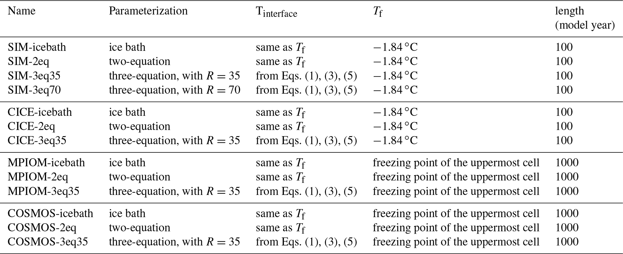
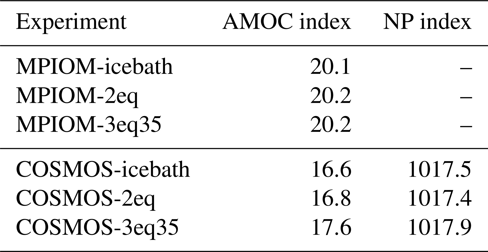
For each model, we perform separate simulations based on the three ice–ocean heat flux formulations (see Table 1). We assume that the three-equation approach with R=35 describes reality more realistically and hence use this simulation as our reference. In our idealized 1-D model, we also use R=70 to test the model sensitivity with respect to this parameter. For a given value of R, we calculate αh to satisfy the requirement described in McPhee et al. (1999). This results in a turbulent heat exchange coefficient αh=0.0095 for R=35 and αh=0.0135 for R=70. In SIM and CICE the mixed-layer salinity has a constant value of 34 g kg−1. In MPIOM and COSMOS the salinity of the seawater evolves dynamically in response to oceanic or atmospheric processes.
Table 1List of experiments. Note that denotes the ratio between turbulent exchange coefficients for heat (αh) and salt (αs).
As atmospheric forcing, we use Eqs. (7) to (9) for our conceptual 1-D model. For CICE, we use the National Center for Atmospheric Research (NCAR) monthly mean climatological data with 1∘ × 1∘ resolution Kalnay et al. (1996). Input fields contain monthly climatological sea surface temperature, sea surface salinity, the depth of ocean mixed layer, surface wind speeds, 10 m air temperature, humidity, and radiation for the time period 1984–2007. For MPIOM, we use a GR30 (about 3∘) horizontal resolution and 40 uneven vertical layers, forced by daily heat, freshwater, and momentum fluxes as given by the climatological Ocean Model Intercomparison Project (OMIP) forcing (Röske, 2006).
For the coupled model COSMOS, the configuration of the ice–ocean component MPIOM is the same as we use for the stand-alone version of this model. The atmospheric module ECHAM5 is used at T31 resolution (3.75∘) with 19 vertical levels. The coupled model was initialized from a pre-industrial simulation and integrated with the solar constant, Earth's orbital parameters, and greenhouse gas forcing all fixed at their 1950 CE values. All simulations were run sufficiently long to reach quasi-equilibrium.
We now turn to a description of the simulated responses of sea ice, ocean, and atmosphere to the three different parameterizations.
5.1 Influence of u*, hmix and ice concentration
We start with a number of sensitivity experiments with our simple 1-D model that were carried out to understand the underlying relationship between simulated ice thickness and the three different parameterizations. We performed four different simulations with our simple model, which in the following are called SIM-icebath, SIM-2eq, SIM-3eq35, and SIM-3eq70, where for the three-equation setup the last number denotes the value of . We run the simulations until the ice reaches its equilibrium thickness, with no more changes from one year to the next.
In our standard SIM simulations we applied m s−1, a sea ice concentration C=85 %, an albedo of seawater αoce=0.1 and a mixed-layer depth hmix=40 m. The sea ice salinity is kept at 0. In winter, when the ocean loses energy to the atmosphere through the open-water part of the grid cell, the simulated heat loss from the ocean is identical in the four setups (Fig. 1c), since their open-water part is identical and the ocean is constantly at its freezing temperature (Fig. 1b). Hence, any heat that is extracted from the mixed layer directly causes ice growth, which explains the very similar accretion rates of the sea ice (Fig. 1a). Major differences between the simulations arise as soon as the net heat flux becomes positive and begins to heat the ocean. All energy that enters the ocean is then directly used to melt the ice in SIM-icebath, while some of the heat is stored in the ocean in SIM-2eq and SIM-3eq. Hence, ice in SIM-2eq and SIM-3eq melts slower than the ice in SIM-icebath, and the ocean remains warmer throughout spring (Fig. 1b). Once the ice in SIM-icebath is melted completely, the ocean temperature rises rapidly and quickly exceeds that in SIM-2eq and SIM-3eq. This can be explained by two facts: (1) in SIM-2eq and SIM-3eq, the sea ice reflects most of the incoming shortwave radiation, and (2) in SIM-2eq and SIM-3eq the heat flux absorbed by open water is primarily used for sea ice melting, while in SIM-icebath no more sea ice exists, such that the entire heat flux into the ocean causes a warming of the seawater. The slower melting of the ice in SIM-2eq and SIM-3eq and the resulting lower heat storage in the ocean throughout summer results in an earlier onset of sea ice formation during autumn.

Figure 1Time series of (a) sea ice thickness (m); (b) ocean temperature (∘C); (c) ocean-to-ice heat flux (W m−2); and (d) ice–ocean interface temperature (∘C) in the experiments SIM-icebath, SIM-2eq, SIM-3eq35, and SIM-3eq70 with friction velocity at 0.002 and ice concentration at 75 %. The model is run into equilibrium.
For SIM-icebath and SIM-2eq, the temperature at the ice–ocean interface is constant at the freezing point of the seawater, which for our choice of Sseawater=34 g kg−1 is around −1.84 ∘C. For SIM-3eq, the interface temperature can be significantly above this value, as the interface freshens through the melting of the comparably fresh sea ice (Fig. 1d).
Comparing SIM-2eq, SIM-3eq35, and SIM-3eq70, we find that the ice thins earlier and faster in SIM-2eq because the ocean heat flux between the ocean and the ice is amplified in this setup, owing to the constantly cold interfacial temperature. Accordingly, the oceanic temperature increases more slowly throughout spring in SIM-2eq. In SIM-3eq70, the transport of salt to the interface is lower than in SIM-3eq35. Hence, the interface remains fresher and warmer throughout summer. Despite the warmer interface, stronger heat fluxes and slightly faster ablation of the ice are simulated, mainly resulting from a higher turbulent heat exchange coefficient αh, which is 0.0095 in SIM-3eq35 and 0.0135 in SIM-3eq70.
To quantify the different response of the simulated sea ice cover for a larger range of forcing conditions, we carried out a series of sensitivity studies. For each of these, we varied one of the forcing parameters and analyzed the difference in annual mean ice–ocean heat flux between SIM-3eq35 and SIM-icebath.
We find that in our simplified setup, differences in ice thickness between SIM-3eq35 and SIM-icebath increase with mixed-layer depth. This is due to the fact that the same amount of heat input causes a smaller temperature change for a deeper mixed layer. According to Eq. (3), a smaller temperature change then leads to a smaller change in heat flux to the ice bottom (Fig. 2).
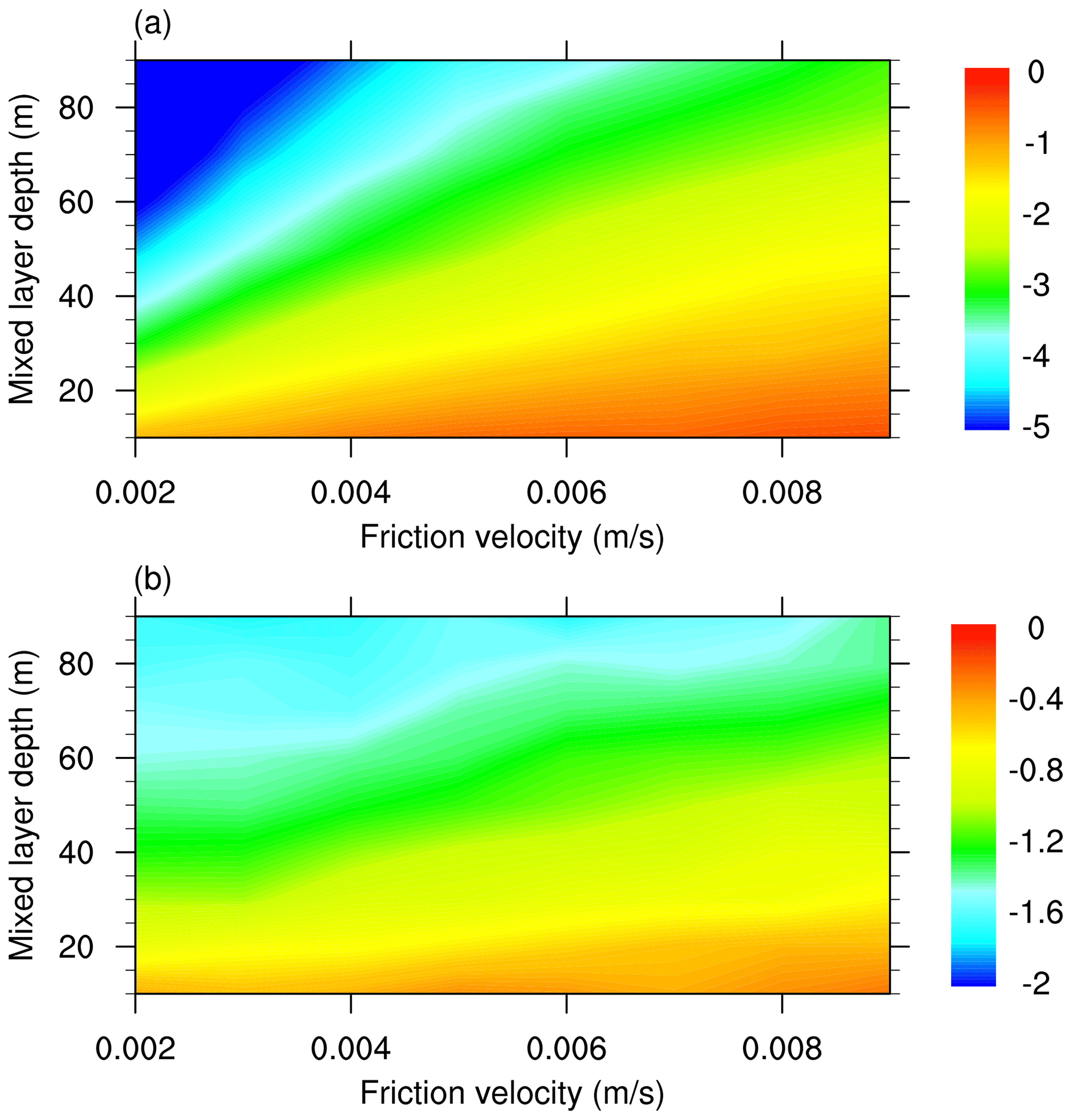
Figure 2Anomalies of ocean-to-ice heat flux in SIM for (a) three-equation minus icebath and (b) three-equation minus two-equation for different choices of mixed-layer depth and friction velocity (units: W m−2).
In addition, we find that the difference in sea ice thickness generally decreases with friction velocity. This is related to the fact that for larger friction velocity more heat is transported to the ice–ocean interface in the three-equation setup (Fig. 2), which enhances sea ice melt.
Finally, regarding sea ice concentration, we find in our simplified setup that differences in ice thickness between SIM-3eq35 and SIM-icebath are larger for a smaller ice concentration. This is related to the fact that the residual energy, which mainly comes from the net incoming heat flux through open water, is all used for ablating sea ice in SIM-icebath, while in SIM-3eq35 only a fraction of the heat is used for ice ablation. Lower ice concentration enhances the energy in the open water and therefore also the difference in the amount of heat transferred to the ice cover.
5.2 Ice thickness
Having understood some of the qualitative impact of the different parameterizations, we can now turn to an analysis of their impact in the more realistic setting provided by CICE, MPIOM, and COSMOS. In these models R=35 is applied in the full three-equation approach. The presented results focus on the Arctic Ocean, as we only find a small response of Southern Ocean properties to the change of ice–ocean heat flux parameterizations, in particular in MPIOM and COSMOS; furthermore, the stand-alone sea ice model CICE simulates an unrealistic distribution of sea ice in warm months in the Southern Ocean, as it fails to capture the heat release from the relatively deep mixed layer.
We let all models run until the modeled ice cover and, in MPIOM and COSMOS the deep-ocean temperatures, reached quasi-equilibrium. More concretely, we performed CICE experiments for 100 model years, with the last 10 years representing its quasi-equilibrium state. For MPIOM and COSMOS, 1000-model-year experiments were conducted, and data from the last 100 model years were used for analysis. The significance level of any differences between the individual simulations was calculated by performing Student's t test, which is used to examine if results from two different parameterizations are significantly different. For the Student's t test, the interannual variances of the last 100 simulation years (10 years in the case of CICE) are considered.
We find that the ice thickness responds similarly to the different parameterizations as it does in the simple one-dimensional model. Everything else unchanged, compared to the three-equation approach the ice bath parameterization leads to thinner ice throughout the Arctic Ocean both in winter and summer (Fig. 3). The change is similar but less pronounced in the simulations based on the two-equation parameterization. The most significant changes occur in the marginal ice zone where sea ice concentration is lowest, again consistent with the results from the one-dimensional model. In the Arctic, the change in March thickness is generally less pronounced than the change in September thickness. This is due to the fact that the air-to-ocean heat flux tends to be negative (the ocean loses heat to the air) in March and because both the temperature of the water and the temperature at the ice–ocean interface are maintained at the freezing point. Hence, in all parameterizations the extracted heat is directly transferred into sea ice formation. In September, in contrast, the ocean can maintain a temperature above the freezing temperature in the two-equation or three-equation approach but not in the ice bath approach. Hence, as in the simple 1-D model, differences between the different parameterizations are more pronounced during summer.
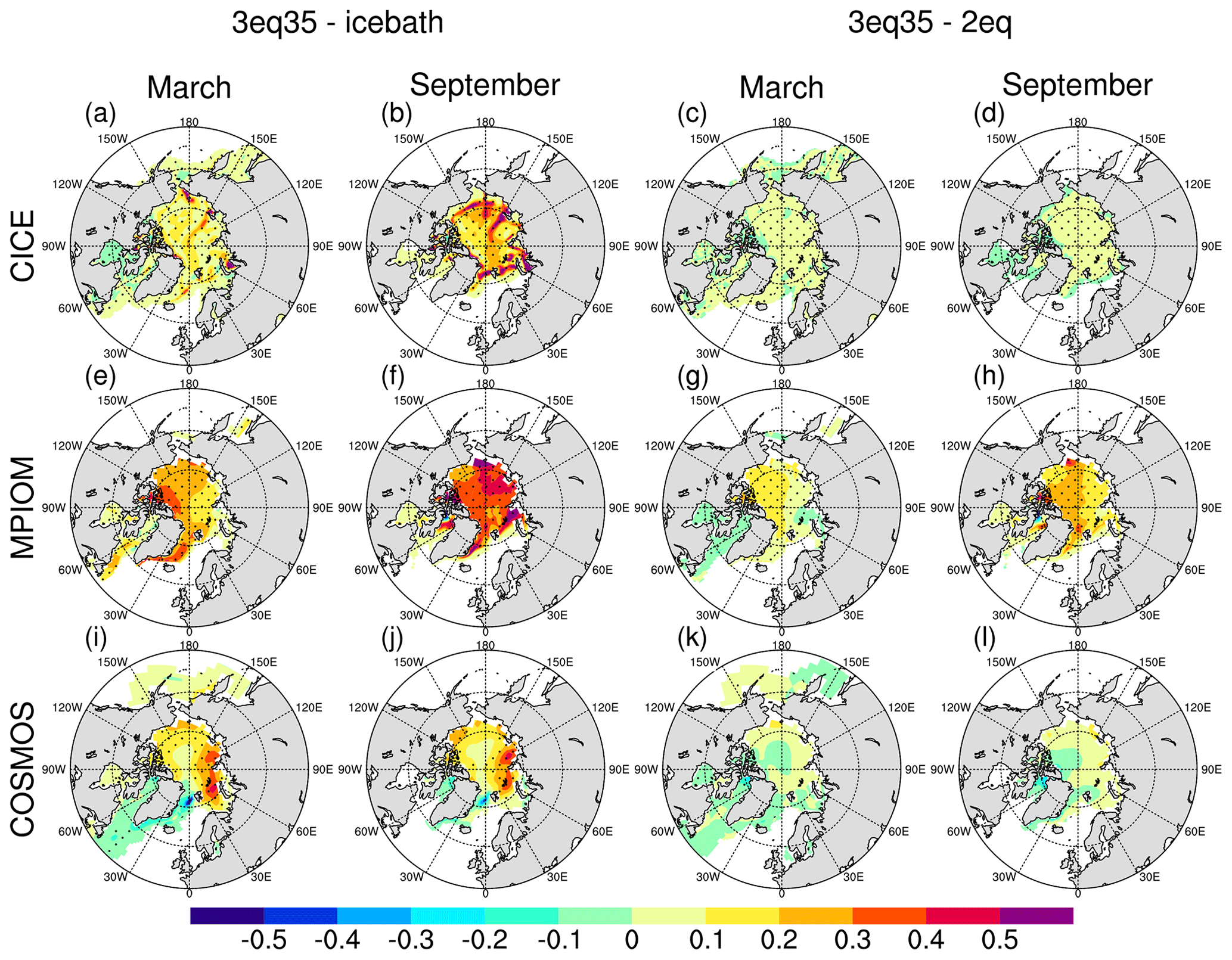
Figure 3The difference in the Arctic sea ice thickness for (a) CICE-3eq35−CICE-icebath in March, (b) CICE-3eq35−CICE-icebath in September, (c) CICE-3eq35−CICE-2eq in March, (d) CICE-3eq35−CICE-2eq in September, (e) MPIOM-3eq35−MPIOM-icebath in March, (f) MPIOM-3eq35−MPIOM-icebath in September, (g) MPIOM-3eq35−MPIOM-2eq in March, (h) MPIOM-3eq35−MPIOM-2eq in September, (i) COSMOS-3eq35−COSMOS-icebath in March, (j) COSMOS-3eq35−COSMOS-icebath in September, (k) COSMOS-3eq35−COSMOS-2eq in March, and (l) COSMOS-3eq35−COSMOS-2eq in September. The marked area has a significance level of greater than 95 % based on Student's t test (units: m).
In addition, sea ice concentration is high throughout March, which reduces the direct interaction of atmospheric heat fluxes with the ocean. As discussed in the previous subsection, this limits differences between the different parameterizations during wintertime. Finally, the ice thins somewhat less in winter because of dynamical effects: the thinner ice is more mobile and more prone to ridging, which fosters the formation of areas with open water. In these areas, significant amounts of new ice can form, which dampens some of the thermodynamic thinning of the ice pack.
In summer, among the three parameterizations only the three-equation approach can result in an ice–ocean interface temperature above the freezing point of the uppermost ocean layer (Fig. 4), which reduces the ocean-to-ice heat flux. This is due to the fact that the ice–ocean interface is usually very fresh, owing to the ablation of the ice bottom. When the temperature of the interface exceeds that of the mixed layer, a reversed heat flux from the ice to the ocean can occur.
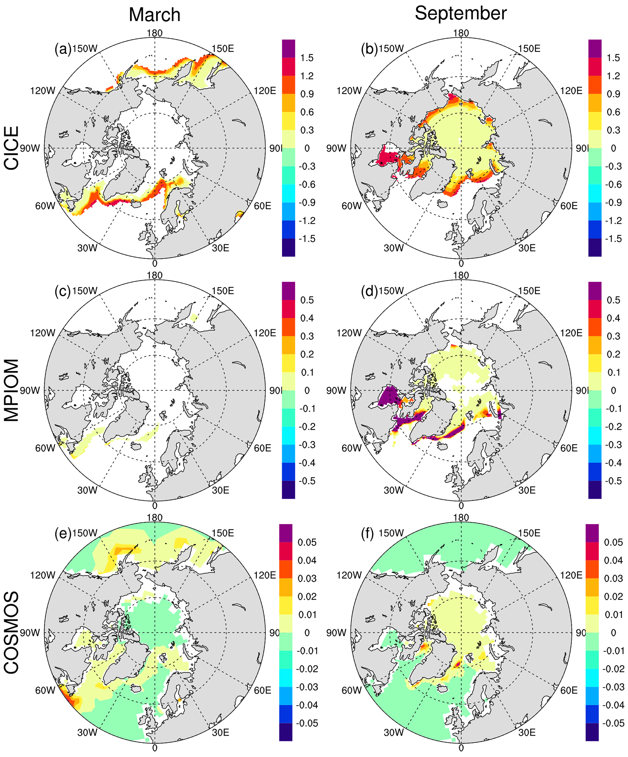
Figure 4The anomaly of the Arctic ice–ocean interface temperature in (a)–(b) CICE-3eq35, (c)–(d) MPIOM-3eq35, and (e)–(f) COSMOS-3eq35 relative to freezing point of the far-field ocean (about ). The left column is for March, and the right column is for September (units: K).
5.3 Upper-ocean temperature and salinity
We now move on to analyze how the described changes in sea ice impact upper-ocean temperature and salinity. We find for the Arctic Ocean that the ice bath parameterization and the two-equation approach result in almost the same temperature distribution during winter as the more realistic three-equation approach in CICE and MPIOM (Fig. 5a, c, e, g). During summer, however, the ice bath approach causes warmer water to persist around the ice edge in CICE (Fig. 5b). This is caused by the fact that here the ice melts earlier than in the three-equation approach, which then allows the ocean to absorb heat more efficiently. The same is found in MPIOM in the areas of Hudson Bay, Baffin Bay, the Norwegian Sea, and the Barents Sea (Fig. 5f, h). The most intriguing feature found in COSMOS is a significant cooling across the North Atlantic Ocean in the ice bath and two-equation parameterizations compared to the three-equation approach (Fig. 5i–l). Such cooling is a consequence of weakened thermohaline circulation, which tends to bring relatively warmer water from the lower latitudes (see Sect. 4.4).
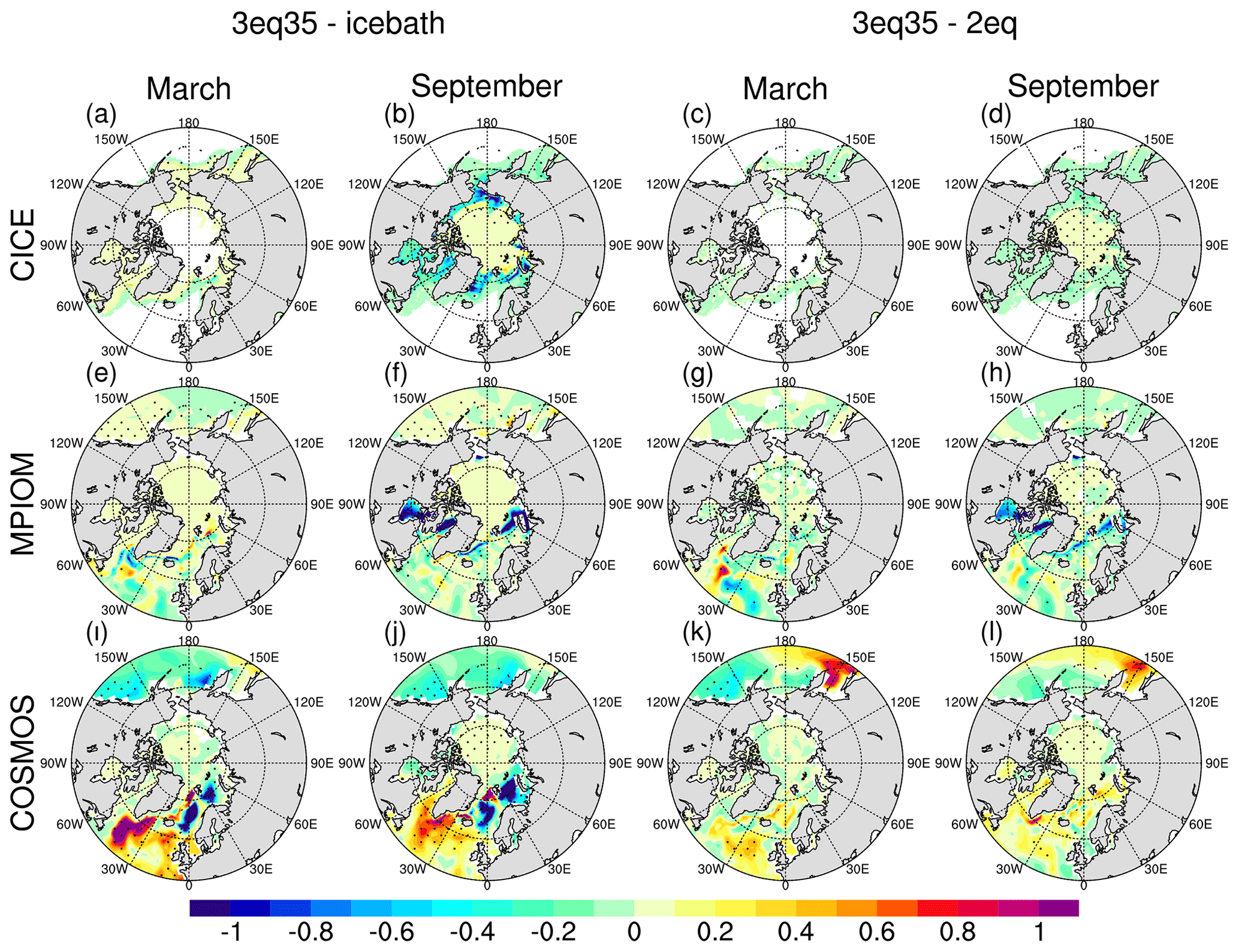
Figure 5As in Fig. 3 but for the sea surface temperature (units: K).
Because brine is released from sea ice during its formation and growth, the changes in ice thickness between different parameterizations should trigger changes in upper-ocean salinity. Indeed, we find such changes to occur (Fig. 6). In regions in which the ice bath approach or the two-equation approach cause an increased heat flux to the ice underside, and hence a larger melting rate of sea ice in summer and a smaller growth rate in winter, the ocean is generally less salty in the simulations with a simplified parameterization of ice–ocean heat exchange than in the simulations with the full three-equation parameterization. Interestingly, the opposite sign is observed in the Barents Sea and its adjacent regions (Fig. 6e–f), despite the larger melt rates in the ice bath scheme. The North Atlantic Ocean experiences a pronounced freshening in the ice bath approach in COSMOS (Fig. 6e–f), which lowers the efficiency of deep-water formation. No significant differences in upper ocean salinity are found between experiments COSMOS-2eq and COSMOS-3eq35 (Fig. 6g–h).
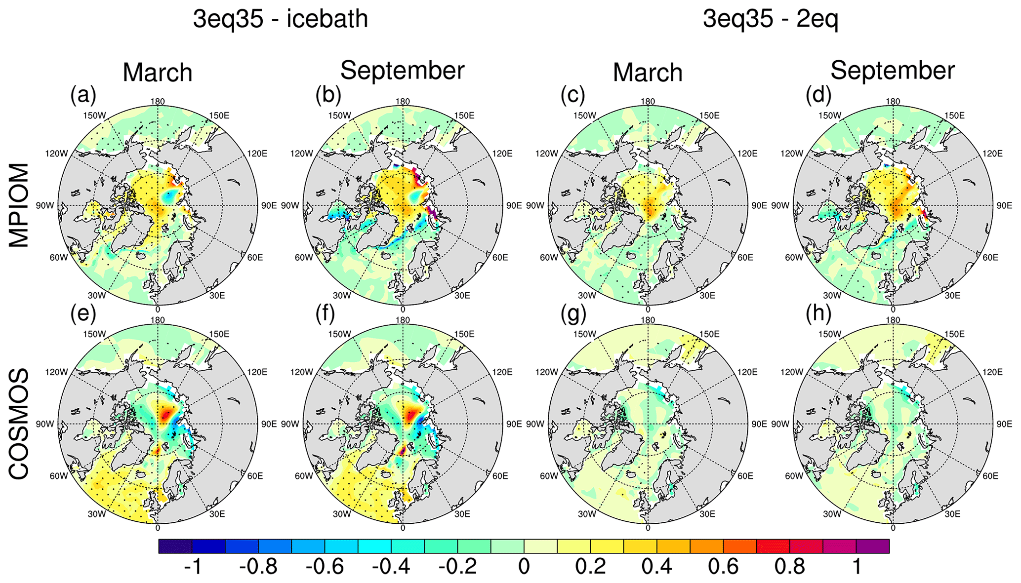
Figure 6As in Fig. 3e–l but for the sea surface salinity (units: g kg−1).
5.4 Thermohaline structure of the ocean
We now turn to the large-scale changes in the thermohaline structure of the ocean. We find that compared to the more realistic three-equation approach, the ice bath and two-equation approaches lead to significant cooling of the ocean's deep-water masses (Fig. 7c, e, g). This behavior is due to the fact that the heat flux out of the ocean is slowed down in the three-equation approach. Hence, more heat can be stored in the mixed layer and further advected into the deep ocean. However, the opposite is found in experiment MPIOM-icebath, which results in a pronounced warming in the deep-water masses by up to 0.5 ∘C (Fig. 7a). This warming in the simulations with the least realistic parameterization of ice–ocean heat exchange reflects the earlier ice loss in the marginal ice zone, which causes enhanced surface warming of the water there.
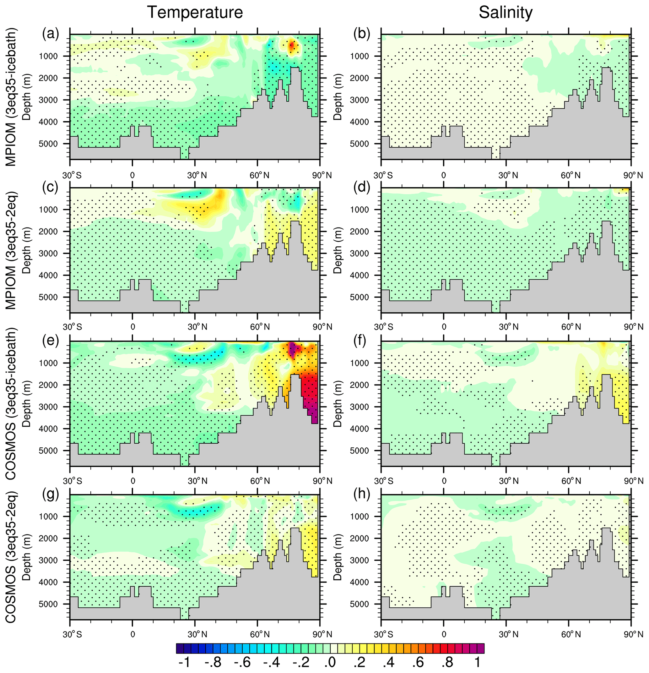
Figure 7Anomalies in zonal mean temperature and salinity vertical profile across the North Atlantic section (−80–0∘ W) for the latitudes from 30∘ S to 90∘ N (a, b) MPIOM-3eq35−MPIOM-icebath, (c, d) MPI-3eq35−MPI-2eq, (e, f) COSMOS-3eq35−COSMOS-icebath, and (g, h) COSMOS-3eq35−COSMOS-2eq. The left column is for temperature, and the right column is for salinity (units: K and g kg−1).
As the simplified parameterizations both lead to faster melting of sea ice in the Arctic Ocean in summer and less growth in winter as compared to the most realistic approach, one would expect a freshening of the ocean mixed layer and the deep-water mass that originates from such fresher surface source water. However, we find that such freshening in MPIOM occurs only within the Arctic upper ocean between depths of 0 and 100 m (Fig. 7b, d). In COSMOS, the freshening extends to the bottom of the Arctic Ocean (Fig. 7f, h). This different model behavior is currently not understood.

Figure 8Anomalies in AMOC (a) MPIOM-3eq35−MPIOM-icebath, (b) MPI-3eq35−MPI-2eq, (c) COSMOS-3eq35−COSMOS-icebath, and (d) COSMOS-3eq35−COSMOS-2eq (units: Sv).
The Atlantic meridional overturning circulation (AMOC) streamfunction, defined as the zonally integrated transport over the Atlantic basin, shows a weakening over 40–60∘ N, 0–3000 m depth in MPIOM-icebath and MPIOM-2eq compared to MPIOM-3eq35. In COSMOS, a pronounced weakening of AMOC is obtained south of 60∘ N. The AMOC index, i.e., the maximum value of the AMOC streamfunction over the region of 800–2000 m depth at 20–90∘ N, is found to be 20.2 and 17.6 Sv in MPIOM-3eq35 and COSMOS-3eq35, respectively (Table 2). The latter is consistent with the estimates of global circulation from hydrographic data (15 ± 3 Sv) (Ganachaud and Wunsch, 2000). Compared to the corresponding three-equation approach, the strength of the AMOC decreases by 1 and 0.8 Sv in COSMOS-icebath and COSMOS-2eq, respectively (Table 2). In COSMOS-icebath, the reduced sea surface salinity in the Atlantic section (Fig. 6e–f, Fig. 7f) lowers the efficiency of deep-water formation, resulting in a weakening of the AMOC (Fig. 8c). A similar but less pronounced pattern is obtained by COSMOS-2eq (Fig. 7h). No significant anomaly in the AMOC index is found in MPIOM (Table 2).
5.5 Atmospheric responses
We now finally turn to investigate how the sea ice changes affect the atmospheric properties in the fully coupled model COSMOS.
The response in surface air temperature, as shown in Fig. 9, indicates a general warming over the Arctic Ocean and its adjacent continents in the COSMOS-icebath and COSMOS-2eq compared to COSMOS-3eq35; a cooling can be found for the Greenland Sea, Nordic Sea, North Atlantic Ocean, southeastern North America, and midlatitude Eurasia. There are various reasons responsible for these changes: (1) reduced Arctic sea ice mass in the ice bath and two-equation approaches lead to a decrease in the surface albedo, resulting in more heat flux absorbed by the surface. (2) The decline of AMOC in experiments COSMOS-icebath and COSMOS-2eq weakens the northward heat transport from lower latitudes to North Atlantic regions. (3) The atmospheric circulation also plays a role, which is discussed in the following.
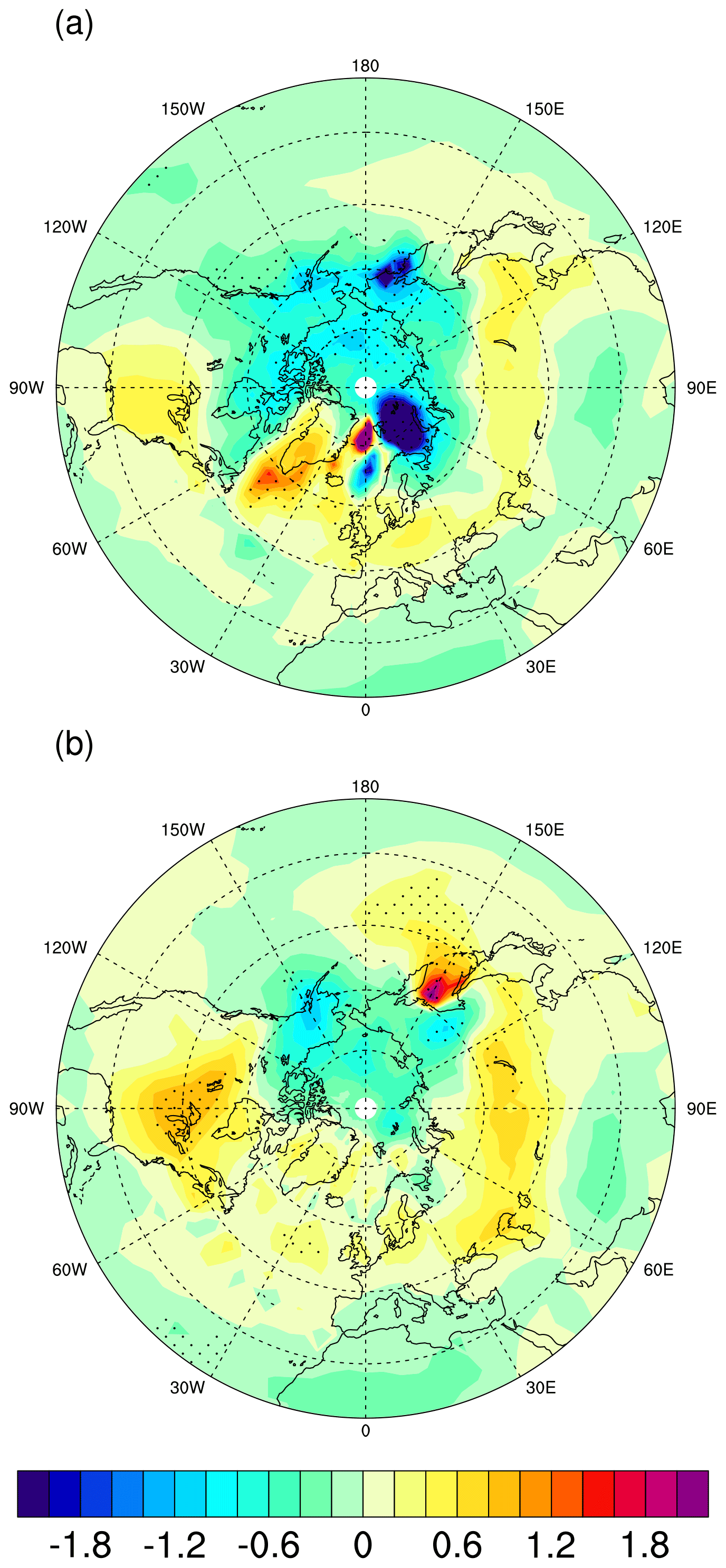
Figure 9Anomalies in surface air temperature (a) COSMOS-3eq35−COSMOS-icebath and (b) COSMOS-3eq35−COSMOS-2eq (units: K).
Figure 10 depicts the responses in boreal winter sea level pressure (SLP). Compared to the most realistic parameterization, the simplified approaches illustrate a more negative North Atlantic Oscillation (NAO) mode, with positive SLP anomalies over the Greenland and Nordic seas and negative anomalies over the North Atlantic subtropical zone. SLP anomalies in another time window show a similar pattern (Fig. S1), indicating the robustness of the NAO signal in the simplified approaches even though the significance level does not exceed 95 %. Composite analysis shows that a positive NAO mode leads to a warming over much of Europe and far downstream as the wintertime enhanced westerly flow across the North Atlantic moves relatively warm and moist maritime air to that region (Fig. S2a). Another notable feature is the cooling and warming over North Africa and North America, respectively, which is associated with the stronger clockwise flow around the subtropical Atlantic high-pressure center. These described patterns are consistent with the modeled surface air temperature response over Northern Hemisphere continents (Fig. 9).
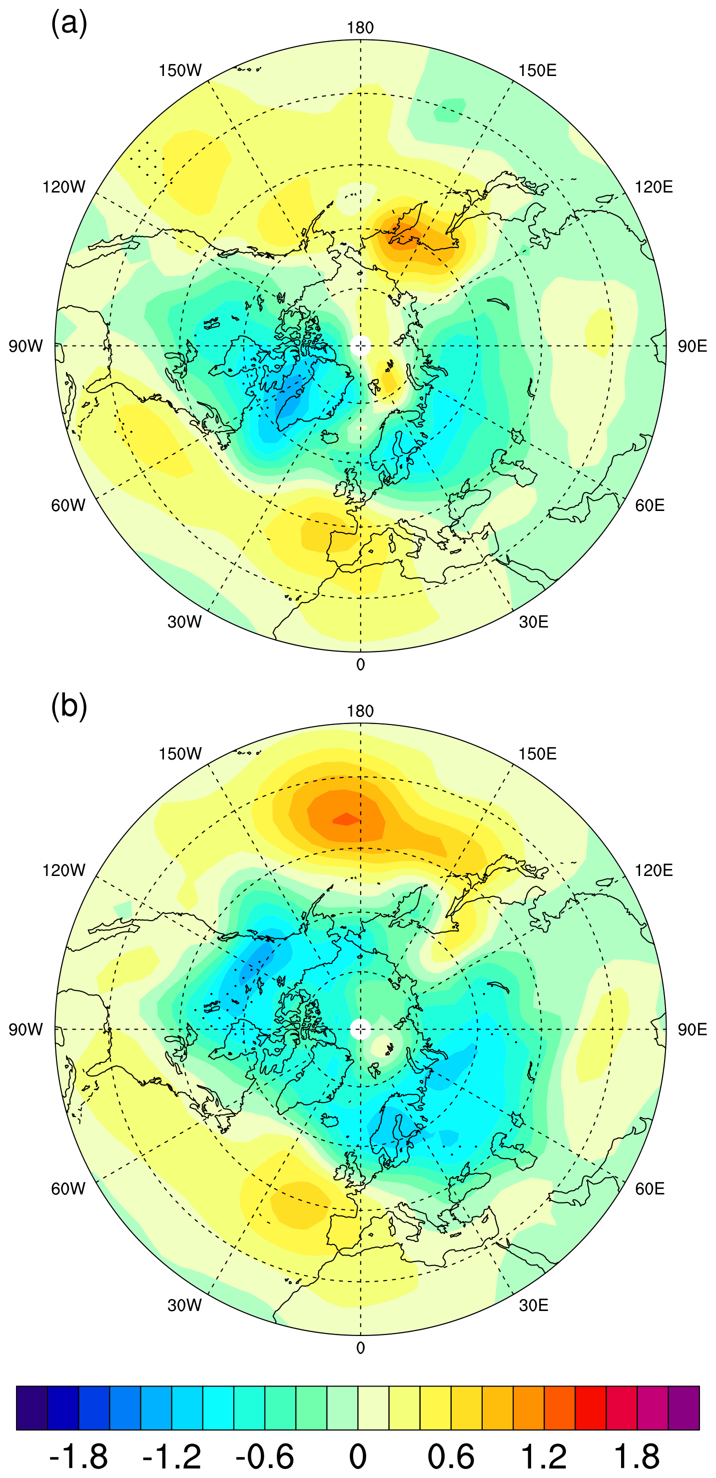
Figure 10Anomalies in boreal winter sea level pressure (a) COSMOS-3eq35−COSMOS-icebath, and (b) COSMOS-3eq35−COSMOS-2eq (units: hPa).
Another intriguing pattern in the atmosphere is an anomalous negative SLP over the North Pacific Ocean in the simplified parameterizations compared to the most realistic approach. Here we calculate the North Pacific (NP) index as the area-weighted SLP over the region of 30–65∘ N, 160∘ E–140∘ W during boreal winter (Trenberth and Hurrell, 1994). The NP index in COSMOS-3eq35 is shown to be 0.4–0.5 hPa higher than its counterparts (Table 2). A high NP index leads to a warming over southern North America and northern Eurasia, as well as a cooling over northern North America (Fig. S2b), resembling the pattern of the surface air temperature anomalies (Fig. 9). Therefore, the response of the surface air temperature in the simplified parameterizations can be attributed to the combined effect of the weakened AMOC and NAO and the enhanced Aleutian Low.
5.6 Air–sea interaction
In this section the mechanism explaining the weakening AMOC in COSMOS-icebath and COSMOS-2eq as compared to COSMOS-3eq35 is explored. It has long been recognized that the NAO variability has an important influence on the AMOC (Curry et al., 1998; Delworth and Zeng, 2016). Variations in the NAO have been hypothesized to play a role in AMOC variations by modifying air–sea fluxes of heat, water, and momentum. A similar relationship between NAO and the AMOC has also been reported for past climate conditions (Shi and Lohmann, 2016; Shi et al., 2020). Here in Fig. 11 we show the results from a composite analysis between the NAO index and the anomalies in mixed-layer depth based on COSMOS-3eq35. It is calculated by averaging March mixed-layer depth anomalies (departure from the mean state) during years when the NAO index exceeds 1 standard deviation.
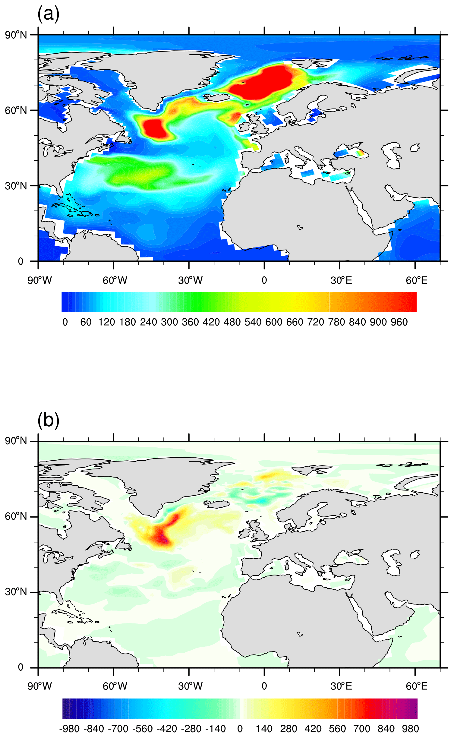
Figure 11(a) Distribution of March mixed-layer depth in COSMOS-3eq35. (b) Composite map of mixed-layer depth and NAO index for COSMOS-3eq35. It is calculated by averaging March mixed-layer depth anomalies (departure from the mean state) during years when the NAO index exceeds 1 standard deviation (units: m).
The convective activities in the Labrador Sea and the Greenland–Iceland–Norwegian (GIN) seas are shown to have important contributions to the production and transport of North Atlantic deep water (Fig. 11a). For comparison, we also show the distribution of mixed-layer depth in MPIOM-3eq35 in Fig. S3, which indicates a different location of the main deep-water convection site to our ice–ocean coupled model: the northeastern North Atlantic. The results from the composite analysis shown in Fig. 11b indicate that the anomalous NAO pattern can lead to significant changes in the ocean circulation. We find that the intensity of the Labrador Sea convection is characterized by variations that appear to be synchronized with variabilities in the NAO. Therefore, the weakening of AMOC in our simplified setups compared to the most realistic approach can be attributed to the simulated anomalous negative NAO phase.
The NAO affects the seawater convection mainly via modifying the surface heat fluxes, which leads to anomalies in the spatial and vertical density gradient. Figure 12a shows the composite map between surface heat flux anomalies and the NAO index. During the positive phase of NAO, more heat than usual is removed from the ocean to the atmosphere in the western Atlantic, in particular from the Labrador Sea. Such a pattern is in good agreement with the NAO-relative heat flux anomalies derived from the European Centre for Medium-Range Weather Forecasts (ECMWF) interim reanalysis (Delworth and Zeng, 2016). The enhanced removal of heat favors an increase in the surface density and thereby strengthens deep-water formation. On the other hand, the NAO also affects the net precipitation over the North Atlantic Ocean. As illustrated in Fig. 12b, relatively dry condition could occur over Labrador Sea and Irminger Sea during positive NAO years.
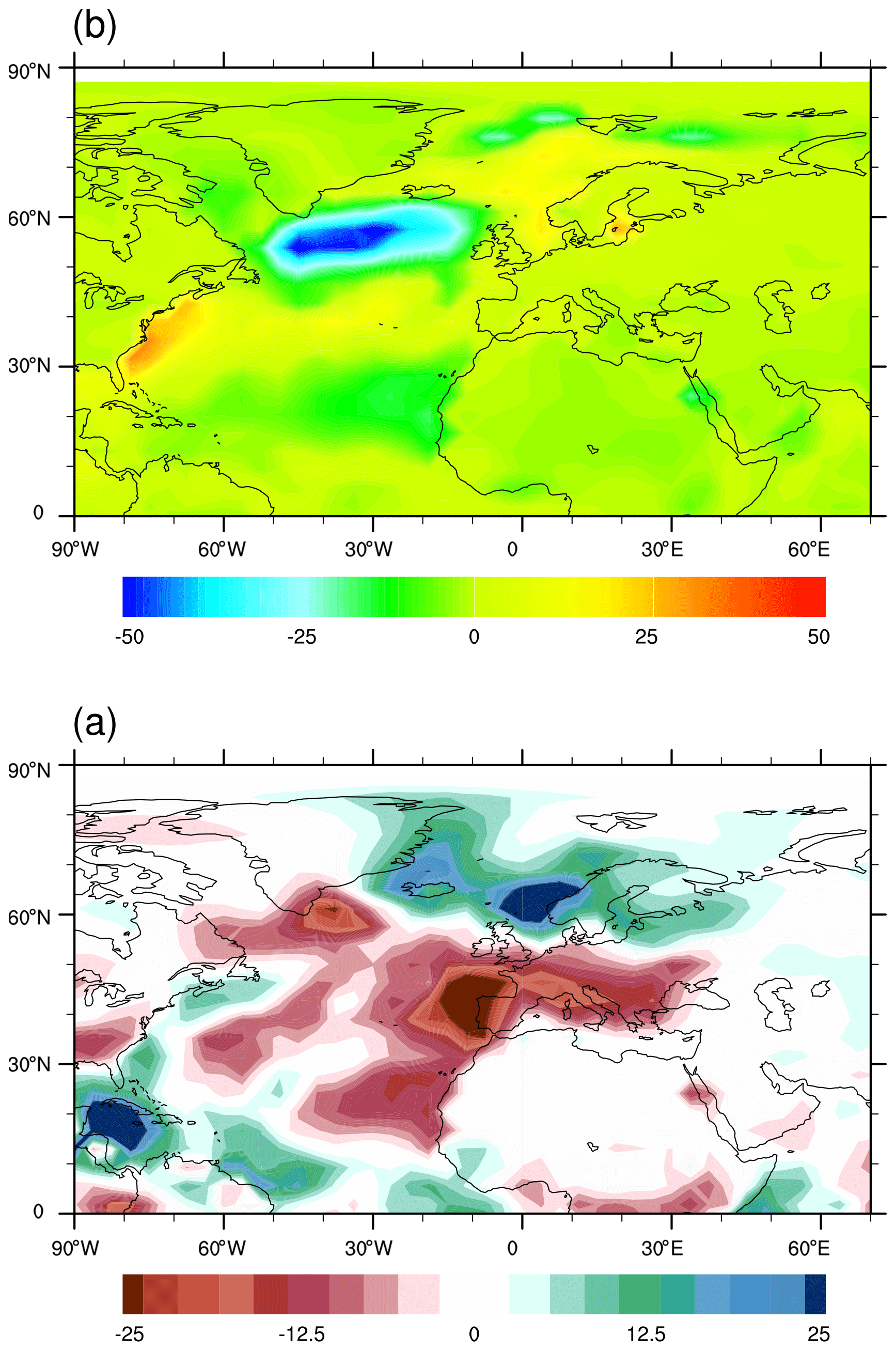
Figure 12Composite map of (a) surface heat flux and (b) net precipitation and NAO index for COSMOS-3eq35. It is calculated by averaging winter anomalies of (a) surface heat flux and (b) net precipitation (departure from the mean state) during years when the NAO index exceeds 1 standard deviation. (units: W m−2 and m).
In the present study, we perform 1-D simulations with an idealized columnar model (SIM), as well as global simulations with a stand-alone sea ice model (CICE), an ice–ocean coupled model (MPIOM), and a fully coupled climate model COSMOS, to analyze the sensitivity of modeled climate to ice–ocean interface heat flux parameterizations. This is achieved by implementing the following elements into the models: (1) a simple ice bath assumption with the ocean temperature fixed at the freezing temperature, (2) a more realistic bulk two-equation approach with freezing temperature kept at the ice–ocean interface where the ocean is allowed to be warmer than freezing point (McPhee, 1992), and (3) a more advanced double diffusional transport (three-equation) approach with the temperature at the ice–ocean interface calculated based on the melting rate of the ice bottom (Notz et al., 2003).
The conclusions drawn from these models in terms of sea ice properties are quite similar to each other. The thinnest ice is observed in the ice bath simulations, as no residual heat is allowed to remain in the ocean and the seawater beneath sea ice is constantly at its freezing point. The two-equation experiments simulate thicker sea ice because some of the heat is stored in the ocean rather than used for ablating the ice. The simulated sea ice by the three-equation approach has the largest thickness, as the temperature at the ice–ocean interface can exceed the freezing point of the far-field ocean, causing the heat flux from the ocean to be reduced or even reversed. The marginal ice areas are found to be highly sensitive to the choice of ice–ocean heat flux parameterizations. In particular, the seawater temperature in the marginal ice zones is largely determined by the onset or retreat of the sea ice.
As a result of the brine release during sea ice formation, the Arctic Ocean is most salty in the three-equation experiment and least salty in the ice bath experiment. The same is found in the deep-water masses due to their coupling with the surface source water. The thermohaline instability obtained from such a salinity profile is responsible for a strengthening of the Atlantic meridional overturning circulation (AMOC) in the coupled simulation with the three-equation approach. Note that our results are in good agreement with a previous study using CICE (Tsamados et al., 2015) that found stronger basal melting of Arctic sea ice, decreased Arctic Ocean salinity, cooling of seawater in the central Arctic, and warming of seawater at the ice edge in the two-equation experiments compared to the three-equation approach in August. However, in their study the effects are more pronounced, possibly because we used different model versions of CICE and different parameters for the ice–ocean heat flux formulations: one example is the value for R, which is 50 in Tsamados et al. (2015) and 35 in our case. In addition, different atmospheric forcings were used in the two studies.
In contrast to their and other previous studies, in our study we do only use a stand-alone sea ice model but also analyze a coupled ice–ocean model and an Earth system model. These allow us to examine the effect of various oceanic heat flux formulations on the deep ocean and atmospheric circulation, as well as their impact on sea ice properties. In our study, COSMOS reveals intensification in both the AMOC and NAO when the most advanced ice–ocean heat flux parameterization is applied. Ocean observations and model simulations show that the changes in the thermohaline circulation during the last century have been driven by low-frequency variations in the NAO via changes in Labrador Sea convection (Latif et al., 2006). More recently, a delayed oscillator model and a climate model suggest that the NAO forces the AMOC on a 60-year cycle (Sun et al., 2015). The strengthening of the AMOC, obtained in our COSMOS-3eq experiment, is likely due to the combined effect of increased thermohaline instability and the anomalous NAO+ mode. In contrast, no obvious response of the AMOC can be found in the MPIOM experiments (Table 2). As indicated in the present paper and many other studies (Curry et al., 1998; Latif et al., 2006; Sun et al., 2015), the AMOC is closely related to the atmospheric processes over the North Atlantic Ocean. One of the key elements controlling the atmospheric circulation over the North Atlantic is the NAO. As the atmospheric forcings are prescribed in MPIOM, there is no difference in the atmospheric state among the MPIOM experiments. Therefore, the prescribed atmospheric forcing largely limits the air–sea interaction feedback.
Our study indicates a less pronounced sea ice response to ice–ocean interface heat flux parameterizations in the fully coupled climate model COSMOS than in the ice–ocean model MPIOM (compare Fig. 3e–h with Fig. 3i–l). This is because the change of the AMOC has a dampening effect on the simulated sea ice anomalies. The strengthening of the AMOC in COSMOS-3eq can lead to a warming over the Northern Hemisphere, especially over the North Atlantic and the Arctic. This hypothesized link between the AMOC and Northern Hemisphere mean surface climate has been documented in an abundance of studies (e.g., Schlesinger and Ramankutty, 1994; Rühlemann et al., 2004; Dima and Lohmann, 2007; Parker et al., 2007). The AMOC-induced warming helps to reduce the sea ice mass over the Arctic and North Atlantic subpolar regions. Indeed, the sea ice across the Greenland Sea and Baffin Bay are found to be thinnest in COSMOS-3eq.
It should be noted that CICE is in many aspects different from the sea ice component in MPIOM. (1) CICE uses the multi-layer approach with a sub-grid-scale ice thickness distribution (Bitz and Lipscomb, 1999), while MPIOM uses zero-layer thermodynamics following Semtner Jr. (1976). (2) A submodel of ice dynamics based on an elastic–viscous–plastic rheology (Hunke and Dukowicz, 1997; Hunke, 2001) is used in CICE, while in MPIOM viscous–plastic dynamics following Hibler III (1979) are used. (3) Different spatial resolutions are used in CICE (1∘) and MPIOM (3∘). (4) CICE is forced by monthly mean climatological data from National Center for Atmospheric Research (NCAR), while the MPIOM experiments are forced by daily fields from the climatological OMIP data set (Röske, 2006). Therefore, the different model behavior between CICE and MPIOM can be explained to a certain extent by the different model configurations.
A detailed comparison of the simulations carried out here with observational data is beyond the scope of our study. However, we note that the sea ice thickness simulated by COSMOS has been evaluated by Notz et al. (2013), who found an overestimation of Arctic sea ice thickness in ECHAM5/MPIOM (i.e., COSMOS) with the ice bath formulation compared to the reanalysis from the Pan-Arctic Ice Ocean Modeling and Assimilation System (PIOMAS) in both winter and summer. Improving the formulation of the ice–ocean heat flux by applying the three-equation approach causes thicker ice and hence further increases this particular model bias. This indicates that the simplified heat flux parameterization partly compensates for other errors in the coupled model setup.
In the present paper, we exclude the responses of the Southern Ocean, as these are much less pronounced than those of the Arctic Ocean. Another reason is the overestimation of the Southern Ocean sea ice extent by the stand-alone sea ice model CICE due to a lack of represented warm deep water.
Our study provides a better understanding of the impact of a realistic representation of ice–ocean heat flux processes in large-scale climate models, including their effect on sea ice, ocean circulation, and the atmosphere. We find that substantial, large-scale climate metrics can emerge from the different parameterizations, highlighting the importance of a careful evaluation of their impact in climate model simulations.
The source code, data, and scripts for plotting the figures in this paper can be downloaded from https://doi.org/10.5281/zenodo.5036700 (Shi, 2021).
The supplement related to this article is available online at: https://doi.org/10.5194/gmd-14-4891-2021-supplement.
DN, JL, and XS developed the original idea for this study. XS and HY contribute to the code modification and model simulation under the supervision of JL (for CICE), DN (for SIM and MPIOM), and GL (for COSMOS). All authors contributed to the data analysis, discussion, and paper writing.
The authors declare that they have no conflict of interest.
Publisher’s note: Copernicus Publications remains neutral with regard to jurisdictional claims in published maps and institutional affiliations.
We would to express our appreciation for the constructive comments from Bruno Tremblay and another anonymous reviewer. In addition, we would like to thank Karl-Hermann Wieners, Helmuth Haak, Xiucheng Wang, and Mirong Song for their technical help with the MPIOM and CICE models, and we would also like to thank Nils Fischer for very interesting discussions.
This research has been supported by the National Key R&D Program of China (grant no. 2018YFA0605901), the Innovation Group Project of Southern Marine Science and Engineering Guangdong Laboratory (Zhuhai) (grant no. 311021008), the Deutsche Forschungsgemeinschaft under Germany’s Excellence Strategy EXC 2037 “CLICCS – Climate, Climatic Change, and Society” (grant no. 390683824), the second phase of PalMod (grant no. 01LP1924B), and the open fund of State Key Laboratory of Loess and Quaternary Geology, Institute of Earth Environment, Chinese Academy of Sciences (grant no. SKLLQG1920).
The article processing charges for this open-access publication were covered by the Alfred Wegener Institute, Helmholtz Centre for Polar and Marine Research (AWI).
This paper was edited by Fabien Maussion and reviewed by Bruno Tremblay and one anonymous referee.
Berliand, M.: Determining the net long-wave radiation of the Earth with consideration of the effect of cloudiness, Izv. Akad. Nauk. SSSR Ser. Geofiz, 1, 64–78, 1952. a
Bitz, C. M. and Lipscomb, W. H.: An energy-conserving thermodynamic model of sea ice, J. Geophys. Res.-Oceans, 104, 15669–15677, 1999. a, b
Curry, R. G., McCartney, M. S., and Joyce, T. M.: Oceanic transport of subpolar climate signals to mid-depth subtropical waters, Nature, 391, 575–577, 1998. a, b
Delworth, T. L. and Zeng, F.: The impact of the North Atlantic Oscillation on climate through its influence on the Atlantic meridional overturning circulation, J. Climate, 29, 941–962, 2016. a, b
Dima, M. and Lohmann, G.: A hemispheric mechanism for the Atlantic Multidecadal Oscillation, J. Climate, 20, 2706–2719, 2007. a
Ganachaud, A. and Wunsch, C.: Improved estimates of global ocean circulation, heat transport and mixing from hydrographic data, Nature, 408, 453–457, 2000. a
Hibler III, W.: A dynamic thermodynamic sea ice model, J. Phys. Oceanogr., 9, 815–846, 1979. a, b
Holland, D. M. and Jenkins, A.: Modeling thermodynamic ice–ocean interactions at the base of an ice shelf, J. Phys. Oceanogr., 29, 1787–1800, 1999. a
Hunke, E. and Dukowicz, J.: An elastic–viscous–plastic model for sea ice dynamics, J. Phys. Oceanogr., 27, 1849–1867, 1997. a, b
Hunke, E. and Lipscomb, W.: CICE documentation and user’s guide, Los Alamos National Laboratory, Los Alamos, USA, 2010. a, b, c, d
Hunke, E. C.: Viscous–plastic sea ice dynamics with the EVP model: Linearization issues, J. Comput. Phys., 170, 18–38, 2001. a, b
Jenkins, A., Hellmer, H. H., and Holland, D. M.: The role of meltwater advection in the formulation of conservative boundary conditions at an ice–ocean interface, J. Phys. Oceanogr., 31, 285–296, 2001. a, b
Josberger, E. G.: Sea ice melting in the marginal ice zone, J. Geophys. Res.-Oceans, 88, 2841–2844, 1983. a
Kalnay, E., Kanamitsu, M., Kistler, R., Collins, W., Deaven, D., Gandin, L., Iredell, M., Saha, S., White, G., Woollen, J., Zhu, Y., Chelliah, M., Ebisuzaki, W., Higgins, W., Janowiak, J., Mo, K. C., Ropelewski, C., Wang, J., Leetmaa, A., Reynolds, R., Jenne, R., and Joseph, D.: The NCEP/NCAR 40-year reanalysis project, B. Am. Meteorol. Soc., 77, 437–472, 1996. a
Latif, M., Böning, C., Willebrand, J., Biastoch, A., Dengg, J., Keenlyside, N., Schweckendiek, U., and Madec, G.: Is the thermohaline circulation changing?, J. Climate, 19, 4631–4637, 2006. a, b
Lipscomb, W. H. and Hunke, E. C.: Modeling sea ice transport using incremental remapping, Mon. Weather Rev., 132, 1341–1354, 2004. a
Marsland, S. J., Haak, H., Jungclaus, J. H., Latif, M., and Röske, F.: The Max-Planck-Institute global ocean/sea ice model with orthogonal curvilinear coordinates, Ocean Model., 5, 91–127, 2003. a
Maykut, G. A. and Untersteiner, N.: Some results from a time-dependent thermodynamic model of sea ice, J. Geophys. Res., 76, 1550–1575, 1971. a, b, c
McPhee, M.: Air-ice-ocean interaction: Turbulent ocean boundary layer exchange processes, Springer Science & Business Media, New York, https://doi.org/10.1007/978-0-387-78335-2, 2008. a, b, c, d
McPhee, M., Morison, J., and Nilsen, F.: Revisiting heat and salt exchange at the ice-ocean interface: Ocean flux and modeling considerations, J. Geophys. Res.-Oceans, 113, C06014, https://doi.org/10.1029/2007JC004383, 2008. a, b, c, d, e
McPhee, M. G.: The upper ocean, in: The geophysics of sea ice, Springer, USA, https://doi.org/10.1007/978-1-4899-5352-0, pp. 339–394, 1986. a
McPhee, M. G.: Turbulent heat flux in the upper ocean under sea ice, J. Geophys. Res.-Oceans, 97, 5365–5379, 1992. a, b, c
McPhee, M. G., Maykut, G. A., and Morison, J. H.: Dynamics and thermodynamics of the ice/upper ocean system in the marginal ice zone of the Greenland Sea, J. Geophys. Res.-Oceans, 92, 7017–7031, 1987. a, b, c
McPhee, M. G., Kottmeier, C., and Morison, J. H.: Ocean heat flux in the central Weddell Sea during winter, J. Phys. Oceanogr., 29, 1166–1179, 1999. a, b
Mellor, G. L., McPhee, M. G., and Steele, M.: Ice-seawater turbulent boundary layer interaction with melting or freezing, J. Phys. Oceanogr., 16, 1829–1846, 1986. a
Notz, D.: Thermodynamic and fluid-dynamical processes in sea ice, PhD thesis, University of Cambridge, Cambridge, UK, 2005. a
Notz, D., McPhee, M. G., Worster, M. G., Maykut, G. A., Schlünzen, K. H., and Eicken, H.: Impact of underwater-ice evolution on Arctic summer sea ice, J. Geophys. Res.-Oceans, 108, 3223, https://doi.org/10.1029/2001JC001173, 2003. a, b, c, d, e, f, g, h
Notz, D., Haumann, F. A., Haak, H., Jungclaus, J. H., and Marotzke, J.: Arctic sea-ice evolution as modeled by Max Planck Institute for Meteorology's Earth system model, J. Adv. Model. Earth Sy., 5, 173–194, 2013. a, b
Oberhuber, J. M.: Simulation of the Atlantic circulation with a coupled sea ice-mixed layer-isopycnal general circulation model. Part I: Model description, J. Phys. Oceanogr., 23, 808–829, 1993. a
Owen, P. and Thomson, W.: Heat transfer across rough surfaces, J. Fluid Mech., 15, 321–334, 1963. a
Parker, D., Folland, C., Scaife, A., Knight, J., Colman, A., Baines, P., and Dong, B.: Decadal to multidecadal variability and the climate change background, J. Geophys. Res.-Atmos., 112, D18115, https://doi.org/10.1029/2007JD008411, 2007. a
Perovich, D., Grenfell, T., Light, B., Richter-Menge, J., Sturm, M., Tucker III, W., Eicken, H., Maykut, G., and Elder, B.: SHEBA: Snow and ice studies CD-ROM, US Army Cold Reg. Res. and Eng. Lab, available at: https://erdclibrary.on.worldcat.org/search?databaseList=&queryString=1122693513#/oclc/1122693513 (last access: 2 August 2021), 1999. a
Perovich, D. K. and Maykut, G. A.: Solar heating of a stratified ocean in the presence of a static ice cover, J. Geophys. Res.-Oceans, 95, 18233–18245, 1990. a
Roeckner, E., Bäuml, G., Bonaventura, L., Brokopf, R., Esch, M., Giorgetta, M., Hagemann, S., Kirchner, I., Kornblueh, L., Manzini, E., Rhodin, A., and Tompkins A.: The atmospheric general circulation model ECHAM 5. PART I: Model description, Max-Planck-Institute for Meteorology, Hamburg, Germany, vol. 349, https://doi.org/10.17617/2.995269, ISSN 0937-1060, 2003. a
Røed, L. P.: A thermodynamic coupled ice-ocean model of the marginal ice zone, J. Phys. Oceanogr., 14, 1921–1929, 1984. a
Röske, F.: A global heat and freshwater forcing dataset for ocean models, Ocean Model., 11, 235–297, 2006. a, b
Rühlemann, C., Mulitza, S., Lohmann, G., Paul, A., Prange, M., and Wefer, G.: Intermediate depth warming in the tropical Atlantic related to weakened thermohaline circulation: Combining paleoclimate data and modeling results for the last deglaciation, Paleoceanography, 19, PA1025, https://doi.org/10.1029/2003PA000948, 2004. a
Schlesinger, M. E. and Ramankutty, N.: An oscillation in the global climate system of period 65–70 years, Nature, 367, 723–726, 1994. a
Schmidt, G. A., Bitz, C. M., Mikolajewicz, U., and Tremblay, L.-B.: Ice–ocean boundary conditions for coupled models, Ocean Model., 7, 59–74, 2004. a, b, c, d
Semtner Jr., A. J.: A model for the thermodynamic growth of sea ice in numerical investigations of climate, J. Phys. Oceanogr., 6, 379–389, 1976. a, b, c
Shi, X.: Code and data for “Sensitivity of Northern Hemisphere climate to ice-ocean interface heat flux parameterizations”, Zenodo [data set], https://doi.org/10.5281/zenodo.5036700, 2021. a
Shi, X. and Lohmann, G.: Simulated response of the mid-Holocene Atlantic meridional overturning circulation in ECHAM6-FESOM/MPIOM, J. Geophys. Res.-Oceans, 121, 6444–6469, 2016. a
Shi, X., Lohmann, G., Sidorenko, D., and Yang, H.: Early-Holocene simulations using different forcings and resolutions in AWI-ESM, Holocene, 30, 996–1015, 2020. a
Sirevaag, A.: Turbulent exchange coefficients for the ice/ocean interface in case of rapid melting, Geophys. Res. Lett., 36, L04606, https://doi.org/10.1029/2008GL036587, 2009. a
Sun, C., Li, J., and Jin, F.-F.: A delayed oscillator model for the quasi-periodic multidecadal variability of the NAO, Clim. Dynam., 45, 2083–2099, 2015. a, b
Trenberth, K. E. and Hurrell, J. W.: Decadal atmosphere-ocean variations in the Pacific, Clim. Dynam., 9, 303–319, 1994. a
Tsamados, M., Feltham, D., Petty, A., Schroeder, D., and Flocco, D.: Processes controlling surface, bottom and lateral melt of Arctic sea ice in a state of the art sea ice model, Philos. T. R. Soc. A, 373, 20140167, https://doi.org/10.1098/rsta.2014.0167, 2015. a, b, c, d, e
Valcke, S.: The OASIS3 coupler: a European climate modelling community software, Geosci. Model Dev., 6, 373–388, https://doi.org/10.5194/gmd-6-373-2013, 2013. a
Yaglom, A. and Kader, B.: Heat and mass transfer between a rough wall and turbulent fluid flow at high Reynolds and Peclet numbers, J. Fluid Mech., 62, 601–623, 1974. a, b