the Creative Commons Attribution 4.0 License.
the Creative Commons Attribution 4.0 License.
 | 28 Jul 2021
APFoam 1.0: integrated computational fluid dynamics simulation of O3–NOx–volatile organic compound chemistry and pollutant dispersion in a typical street canyon
Luolin Wu
Jian Hang
Xuemei Wang
Min Shao
Cheng Gong
Urban air quality issues are closely related to human health and economic development. In order to investigate street-scale flow and air quality, this study developed the atmospheric photolysis calculation framework (APFoam 1.0), an open-source computational fluid dynamics (CFD) code based on OpenFOAM, which can be used to examine microscale reactive pollutant formation and dispersion in an urban area. The chemistry module of APFoam has been modified by adding five new types of reactions, which can implement the atmospheric photochemical mechanism (full O3–NOx–volatile organic compound chemistry) coupled with a CFD model. Additionally, the model, including the photochemical mechanism (CS07A), air flow, and pollutant dispersion, has been validated and shows good agreement with SAPRC modeling and wind tunnel experimental data, indicating that APFoam has sufficient ability to study urban turbulence and pollutant dispersion characteristics. By applying APFoam, O3–NOx–volatile organic compound (VOC) formation processes and dispersion of the reactive pollutants were analyzed in an example of a typical street canyon (aspect ratio ). The comparison of chemistry mechanisms shows that O3 and NO2 are underestimated, while NO is overestimated if the VOC reactions are not considered in the simulation. Moreover, model sensitivity cases reveal that 82 %–98 % and 75 %–90 % of NO and NO2, respectively, are related to the local vehicle emissions, which is verified as the dominant contributor to local reactive pollutant concentration in contrast to background conditions.
In addition, a large amount of NOx emissions, especially NO, is beneficial to the reduction of O3 concentrations since NO consumes O3. Background precursors (NOx/VOCs) from boundary conditions only contribute 2 %–16 % and 12 %–24 % of NO and NO2 concentrations and raise O3 concentrations by 5 %–9 %. Weaker ventilation conditions could lead to the accumulation of NOx and consequently a higher NOx concentration but lower O3 concentration due to the stronger NO titration effect, which would consume O3. Furthermore, in order to reduce the reactive pollutant concentrations under the odd–even license plate policy (reduce 50 % of the total vehicle emissions), vehicle VOC emissions should be reduced by at least another 30 % to effectively lower O3, NO, and NO2 concentrations at the same time. These results indicate that the examination of the precursors (NOx and VOCs) from both traffic emissions and background boundaries is the key point for understanding O3–NOx–VOCs chemistry mechanisms better in street canyons and providing effective guidelines for the control of local street air pollution.
- Article
(9309 KB) - Full-text XML
- BibTeX
- EndNote


With the rapid urbanization worldwide, air pollution in cities, such as haze and photochemical smog characterized by high levels of particulate matter and/or surface ozone (O3), has become one of the most concerning global environmental problems (Lu et al., 2019; Wang et al., 2020). Recently, observational data have shown that PM2.5, one of the major pollutants in cities, has decreased by 30 %–50 % across China due to strict air quality control measures (Zhai et al., 2019). At the same time, 87 %, 63 %, 93 %, 78 %, and 89 % of the observational stations in China have shown a decreasing trend for CO, NO2, SO2, PM10, and PM2.5 over the last 5 years, respectively (Fan et al., 2020). Various data indicate that air quality in China has been significantly improved. Unlike other pollutants, however, O3 concentrations have increased in major urban clusters of China (Lu et al., 2018). Severe O3 pollution episodes still exist and happen frequently (Wang et al., 2017). Therefore, research into reactive pollutants such as O3, which has adverse effects on human health (Goodman et al., 2015; H. Liu et al., 2018; Sousa et al., 2013), crops (Rai and Agrawal, 2012), building materials (Massey, 1999), and vegetation (Yue et al., 2017), is of great significance to the further improvement of air quality, especially in urban areas.
From the perspective of the cause of urban air pollution, traffic-related emissions are the major part of airborne pollutant sources, including the precursors of O3, NOx (= NO + NO2), and volatile organic compounds (VOCs) (Degraeuwe et al., 2017; Kangasniemi et al., 2019; Keyte et al., 2016; Pu and Yang, 2014; Wild et al., 2017; Wu et al., 2020). It is believed that the production of O3 comes from NO2 photolysis. Generally, in a clean atmosphere, the produced O3 would be consumed by the NO titration effect. However, with the involved VOCs, NO concentrations become lower due to the consumption of RO2 (the production of VOCs and OH, ), which weakens the NO titration effect and consequently leads to O3 accumulation (Seinfeld and Pandis, 2016). In China, previous studies have shown that 22 %–52 % of total CO, 37 %–47 % of total NOx, and 24 %–41 % of total VOC emissions are contributed by vehicle emissions in urban areas (Li et al., 2017; Zhang et al., 2009; Zheng et al., 2014, 2009).
Numerical simulation using air quality models is considered an effective method to investigate the formation pattern and dispersion of reactive pollutants. Based on length scales, the air flow and air quality modeling in cities are commonly categorized into four groups, i.e., street scale (∼100 m), neighborhood scale (∼1 km), city scale (∼10 km), and regional scale (∼100 km) (Britter and Hanna, 2003). Due to the complex geometry and nonuniformity in building distribution within cities, computational fluid dynamics (CFD) simulation has recently gained popularity in the urban climate research (Toparlar et al., 2017). Different from the typical mesoscale (∼1000 km) and regional-scale (∼100 km) air quality models, CFD has better performance in microscale pollutant dispersion within the urban street canyon (∼100 m) or urban neighborhoods (∼1 km), which are restricted spaces with more complicated turbulent mixing and poorer ventilation conditions than rural areas (Zhong et al., 2015). Besides the shorter physical processes in microscale urban models (∼100 m–1 km, ∼10–100 s), the rather fast chemical processes of NO2 photolysis and NO titration with the complex chain of VOC reactions also require finer-resolution models (Vardoulakis et al., 2003). For instance, CFD models with fine grids (∼0.1–1 m) and small time steps (∼0.1 s) have been effectively adopted to simulate these high-resolution spatial and temporal variations in urban areas (Sanchez et al., 2016).
Table 1Overview of the CFD studies with their photochemical mechanisms.
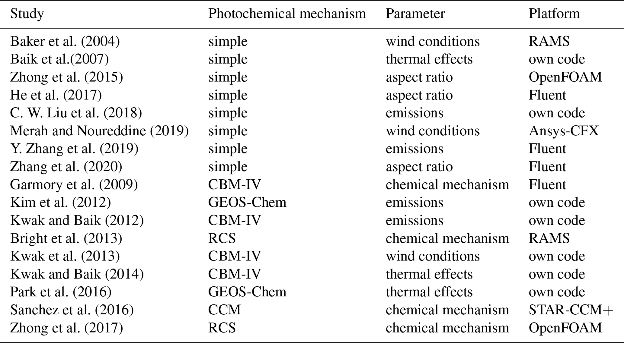
With the rapid growth of the high-performance computing (HPC) platforms, computational power is no longer an obstacle. CFD simulation shows the good application prospects for urban microclimate research (Fernandez et al., 2020; Garcia-Gasulla et al., 2020). Many CFD models coupled with photochemical reaction mechanisms have been developed to investigate the street-scale air quality problem in recent years (see Table 1). More commonly, simple photochemical mechanisms with only three reactions (Leighton, 1961) are adapted in CFD models. This mechanism can simulate the NOx and O3 dispersion with a lower computational requirement. Many previous studies have investigated the pivotal factors that affect the reactive pollutant distribution within the street canyon by using a CFD model with a simple photochemical mechanism, such as a street–building aspect ratio (He et al., 2017; Zhang et al., 2020; Zhong et al., 2015), ambient wind conditions (Baker et al., 2004; Merah and Noureddine, 2019), thermal effects (Baik et al., 2007), or emissions from vehicles (C. W. Liu et al., 2018; Y. Zhang et al., 2019). However, due to the simple photochemical mechanism ignoring the effect of other nitrogen oxides and VOCs on the photochemistry, some studies have recently applied the full photochemical mechanism in CFD models to reduce the uncertainty of pollutant simulation. Photochemical mechanisms contain NOx–O3–VOC reactions and photochemistry, such as CBM-IV (Garmory et al., 2009; Kwak et al., 2013; Kwak and Baik, 2012, 2014), GEOS-Chem (Kim et al., 2012; Park et al., 2016), RCS (Bright et al., 2013; Zhong et al., 2017), and CCM (Sanchez et al., 2016) and are successfully coupled with CFD models and applied to analyze the street-scale pollutant dispersion.
Currently, most of the simulation studies have been carried out via the application of commercial CFD software. This software is rather simple to operate, which is effective in saving time when setting up the simulation case. However, the commercial codes are usually closed source, which is a “black box” for users (Chatzimichailidis et al., 2019). In this case, adjustments to the equations and parameters or modifications to the model are difficult for some specific simulations. Therefore, an open-source CFD code for atmospheric photolysis calculation, APFoam 1.0, was developed in this study. Open-Source Field Operation and Manipulation (OpenFOAM) was selected as the platform for the APFoam framework, as OpenFOAM has good performance regarding computing scalability and low uncertainty levels, which shows its applicability for large-scale CFD simulations with million-level grid numbers (Robertson et al., 2015). In addition, the solvers in OpenFOAM for specific CFD problems can be developed by using the appropriate packaged functionality, which simplifies the difficulty of programming. Furthermore, OpenFOAM has also been developed with various pre- and post-processing utilities that are convenient for data manipulation (OpenFOAM Foundation, 2018).
This paper is organized as follows. Section 2 presents a full description of the new chemistry module and simulation solver. Model validation for the photochemical mechanism, turbulence simulation, and pollutant dispersion compared with the chemical box model and several wind tunnel experiments is discussed in Sect. 3. In Sect. 4 a series of sensitive cases have been set up to investigate the contribution of the key factors to the reactive pollutants in a typical street canyon (aspect ratio of building height to street width, ). Finally, the conclusion and future research plans for the APFoam framework are summarized in Sects. 5 and 6.
2.1 General overview
The APFoam framework has been developed based on OpenFOAM, which is an open-source code for CFD simulation. For the numerical solution, APFoam uses finite-volume method (FVM) to discretize the governing equations and adopts arbitrary three-dimensional structured or unstructured meshes. All variables of the same cell are stored at the center of the control volume (CV), and complex geometries can be easily handled with FVM (Chauchat et al., 2017). In APFoam, laminar, Reynolds-averaged Navier–Stokes equation (RANS), and large-eddy simulation (LES) methods are available for turbulence solution. Additionally, APFoam also has complete boundary conditions to choose from for numerical simulations.
Based on OpenFOAM, APFoam has been developed to conduct photochemical simulations within the atmosphere. Different from the general chemical reaction types, there are some new types of gaseous reactions for describing photochemical processing. More details will be introduced in Sect. 2.2.
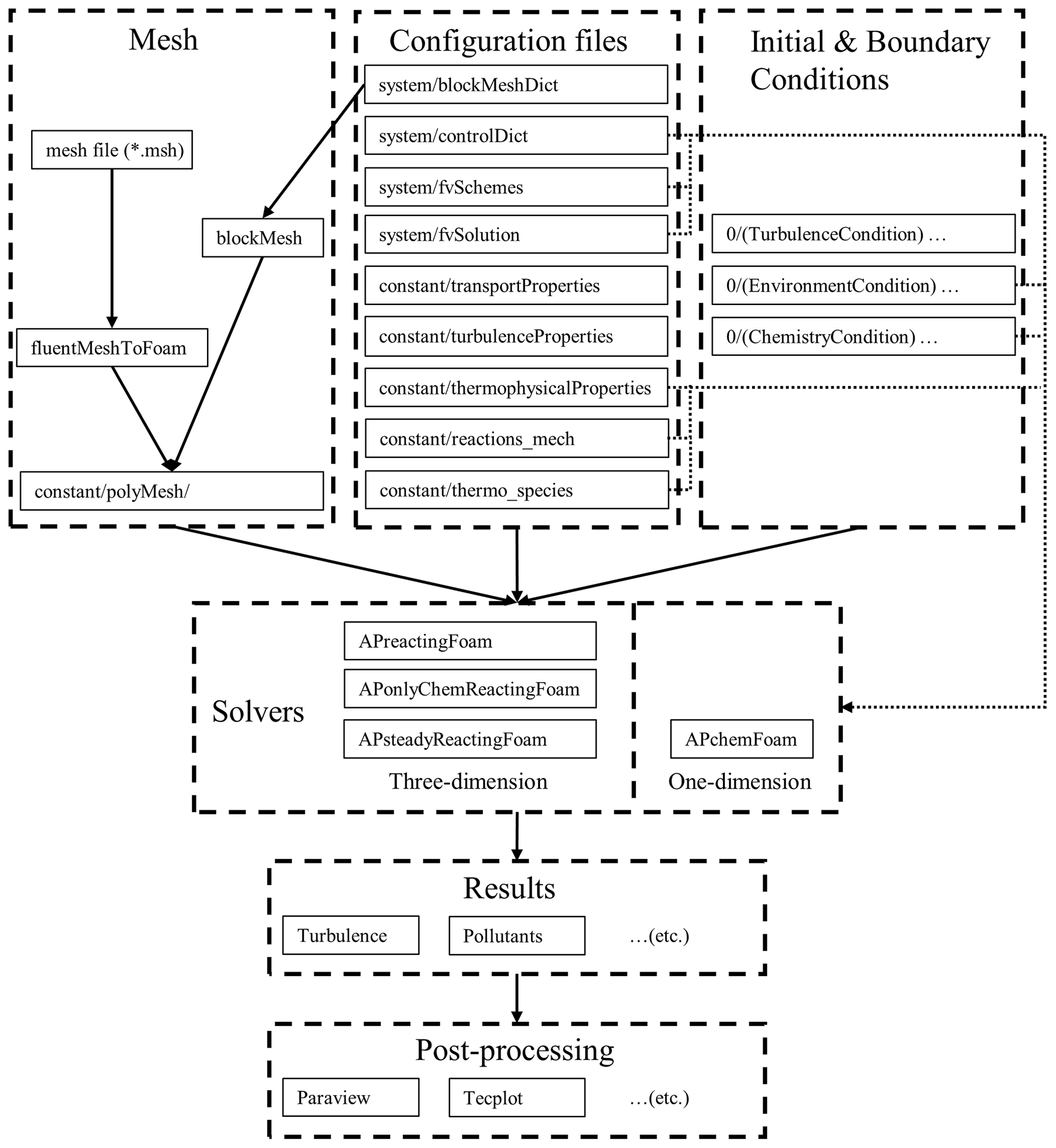
To make it easier to get started with APFoam, the structure of the simulation case folder is consistent with OpenFOAM. Figure 1 shows the flow diagram of the simulation setup in APFoam. The solver of APFoam, APChemFoam for one-dimensional (1D) chemistry solving, is modified from the solver ChemFoam, which will be introduced in detail in Sect. 2.3. Other three-dimensional (3D) solvers are modified from the solver reactingFoam, including APreactingFoam, solving flow field and chemical reactions simultaneously in one time step; APonlyChemReactingFoam, solving only chemical reactions with a certain flow field; and APsteadyReactingFoam, solving flow field and chemical reactions simultaneously in steady state. More details will be presented in Sect. 2.4.
For running the simulation (see Fig. 1), mesh files, configuration files, and initial and boundary condition files should be prepared before the simulation. Mesh files can be made in various ways, such as making a blockMesh application executable by using data from blockMeshDict or fluentMeshToFoam and converting the .msh file to OpenFOAM format. For the APFoam simulation, all required configure files are also listed in Fig. 1. In addition, user-defined functions can be loaded during the run time without recompiling the program via writing-related configuration files in the system folder. As for initial conditions, the initial states of turbulence, the environment (e.g., temperature, pressure), and chemical species are necessary for the simulation. The results of APFoam contain the wind flow and pollutant concentrations, which can be processed by the Paraview in OpenFOAM or any other CFD post-processing tools.
2.2 Chemistry module
For photochemical calculation, there are five types of reactions in the NOx–O3–VOC mechanism. In the original version of OpenFOAM, these types of reactions are not included and should be added to the chemistry module prior to simulation. These types of the reactions are described as follows.
-
Arrhenius reactions.
Arrhenius reactions are the basic reaction in the mechanism, and the rate of the Arrhenius reaction is calculated as
where A, B, and E are the parameters of the reaction rates and T is the temperature of the mixture in degrees kelvin.
-
Photolysis reactions.
Photolysis reactions are first-order reactions, and the photolysis rate is calculated as
where kphot is the first-order rate for the photolysis reaction; λ1 and λ2 are the photolysis wavelength ranges according to the specific species; and J (λ), abs (λ), and QY (λ) are the intensity of the light source, absorption cross section, and the quantum yield for the reaction at wavelength λ, respectively.
In reality, the photolysis rate could be calculated by other photolysis rate models, such as Fast-J (Wild et al., 2000) or TUV (Madronich and Flocke, 1999), or obtained from a photolysis data set, such as IUPAC (Atkinson et al., 2004). Since the photolysis rate does not depend on temperature, in the current version of APFoam the model does not consider the variation of light intensity, and the photolysis rates are obtained from the literature (Carter, 2010) rather than online calculation in order to improve calculation efficiency.
-
Falloff reactions.
The rate of falloff reactions is a function of temperature and pressure that is calculated as follows:
where , [M] is the concentration of third body, which depends on total pressure, and F is the broadening factor. k0 and kinf are the rates of the Arrhenius form at the low-pressure limit and high-pressure limit, respectively.
-
Three-k reactions.
The rate of “three-k” reactions depends on three reaction rates in Arrhenius form. The rate is calculated as
where k0, k2, and k3 are the three reaction rates and [M] is the concentration of third body.
-
Two-k reactions.
The rate of “two-k” reactions depends on two reaction rates in Arrhenius form. The rate is calculated as
where k1 and k2 are the two reaction rates and [M] is the concentration of third body.
In the current version of APFoam, two atmospheric photochemical mechanisms are included in the model, SAPRC07 (Carter, 2010) and CB05 (Yarwood et al., 2005). For SAPRC07, two versions of the chemical mechanism are available, which are CS07A and SAPRC07TB. CS07A is one of the condensed versions of the mechanism, which contains 52 species and 173 reactions. SAPRC07TB is a more complicated version and even contains toxic species, with 141 species and 436 reactions. As for CB05, a basic version with 51 species and 156 reactions is optional in the model. In Sect. 3.1, CS07A has been validated, while the other two mechanisms are not verified in this study but are still an available option for users.
2.3 One-dimensional chemical solver (APchemFoam)
In the APFoam framework, a one-dimensional chemistry solver (i.e., chemistry box model) called APchemFoam is included in the model. This solver only concerns the chemical concentration and reaction heat variation during simulation, and calculations are started from initial conditions within a single cell mesh. The concentration and energy equation are described as follows (OpenFOAM Foundation, 2018):
where Yi is the species mass fraction, ki is the reaction rate, T is the temperature of the mixture, h is the specific enthalpy, u0 is the initial energy, p is the pressure, ρ is the density of the mixture, is the heat from reaction, and Cp,i are the enthalpy of formation at reference temperature T0 and the constant pressure-specific heat (a function of temperature) of species i, R is the gas constant, Mave is the average molar weight, and pi and Mi are partial pressure and the molar mass of species i. In addition, either p or ρ should be set as a constant for the simulation according to the needs of research. The other is calculated by Eq. (9).
2.4 Three-dimensional (3D) CFD solver with photochemical reaction
As mentioned above, three 3D solvers for atmospheric photochemical CFD calculation, including APreactingFoam, APonlyChemReactingFoam, and APSteadyReactingFoam, are developed in the APFoam framework.
For APreactingFoam, flow field, chemical reaction, and pollutant dispersion are solved simultaneously in the same time step in this solver. Firstly, the continuity-governing equation in this solver is
Besides, the momentum governing equation is
Additionally, the energy governing equation is
where U is the velocity vector of the air flow, τ is the viscous stress tensor, K is the specific kinetic energy, and αeff is the effective thermal diffusivity coefficient.
Pressure–velocity coupling schemes for solving the flow field use the PIMPLE algorithm, a merged PISO–SIMPLE algorithm in OpenFOAM toolkit. This algorithm uses a steady-state solution (SIMPLE algorithm) for the flow field within the time step. When the defined tolerance criterion is reached, this algorithm uses the PISO algorithm in the outer correction loop and moves on in time (Holzmann, 2017). The PIMPLE algorithm allows for larger Courant numbers (Co>1) so that the time step can be increased to reduce the computation time. Even so, the time step (Δt) generally follows the Courant–Friedrichs–Lewy (CFL) condition to maintain numerical stability, which is as follows:
where Δx is the grid size.
Besides, the governing equation for the reactive species transportation is
where μ is the kinematic viscosity and is the concentration change of species i from the chemical reaction. As mentioned above, is calculated following Eqs. (6)–(9). Ei is the emission source of species i. The chemistry is solved by the ordinary deferential equation (ODE) solvers in OpenFOAM library, in which the chemical reactions can be integrated by automatically dividing the flow time step into several time sub-steps. The APreactingFoam is only designed to solve compressible fluids because the simulation results are more likely to be unstable and divergent when the chemistry and flow field are solved simultaneously under the incompressible fluids. This is a limitation of OpenFOAM code that is widely known by its users.
APonlyChemReactingFoam is only capable of solving the chemical reaction and species dispersion in the same time step under a certain flow field. The solution of turbulent fluids governing the equation is switched off. The purpose of developing this solver is to save computation time and reduce repetitive simulations. In general, the atmospheric chemical reactions have negligible effect on the flow field. Therefore, when the example cases to be studied do not involve the flow field change, this solver is suitable for this kind of simulation. The governing equation for the reactive species transportation is consistent with APreactingFoam (Eq. 14).
APSteadyReactingFoam is developed for solving the chemical reaction and species dispersion under the steady-state flow field. This solver is only designed to solve compressible fluids for the same reason as APreactingFoam. In this solver, a pressure–velocity coupling scheme switches to a SIMPLE algorithm for steady-state solution. The continuity governing equation in this solver is
Besides, the momentum governing equation is
In addition, the energy governing equation is
As for reactive species, the governing equation for the transportation still applies Eq. (14) as well in order to ensure the stability of chemical reaction.
3.1 Photochemical reaction mechanism
To verify the accuracy of the chemical reaction solution and species concentration calculation, APFoam results are compared with the results from SAPRC box modeling software (Carter, 2010). For the chemical mechanism, CS07A is selected for validation in this study, and the simulation time is set to 24 h without diurnal variation (i.e., the chemical reaction rate is constant during the simulation), allowing the reactants to fully react and verifying the stability of the model.
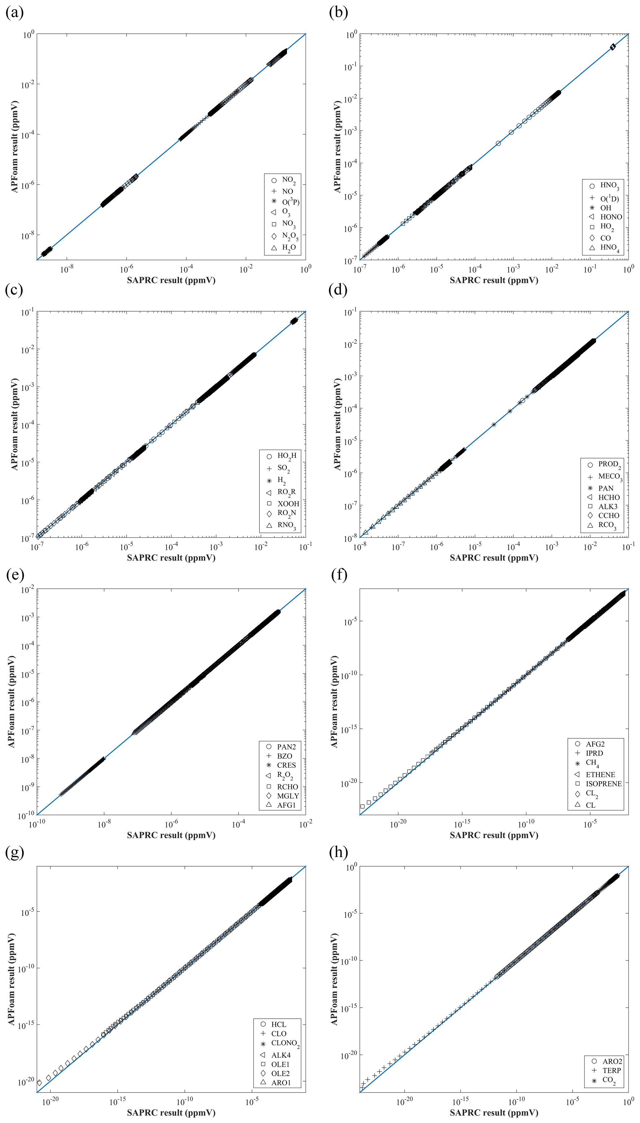
Figure 2 shows the concentrations of 52 species from two models at 24 h, which is the last time step of the simulation. In general, APFoam results have a good agreement with the SAPRC box model. The simulation results for other species from two models are basically consistent, except that some species have large errors when the magnitude is very small (Fig. 2f–h).
For further investigation, relative error (RE, %) for each species at each time step and mean relative error (MRE, %) are calculated for the selected species with large bias. These statistics are calculated as follows:
where REi,t is the relative error of species i at time step t, is the concentrations of species i at time step t from APFoam, is the concentrations of species i at time step t from SAPRC box model, MREi is the mean relative error of species i, and n is the total number of the time step.
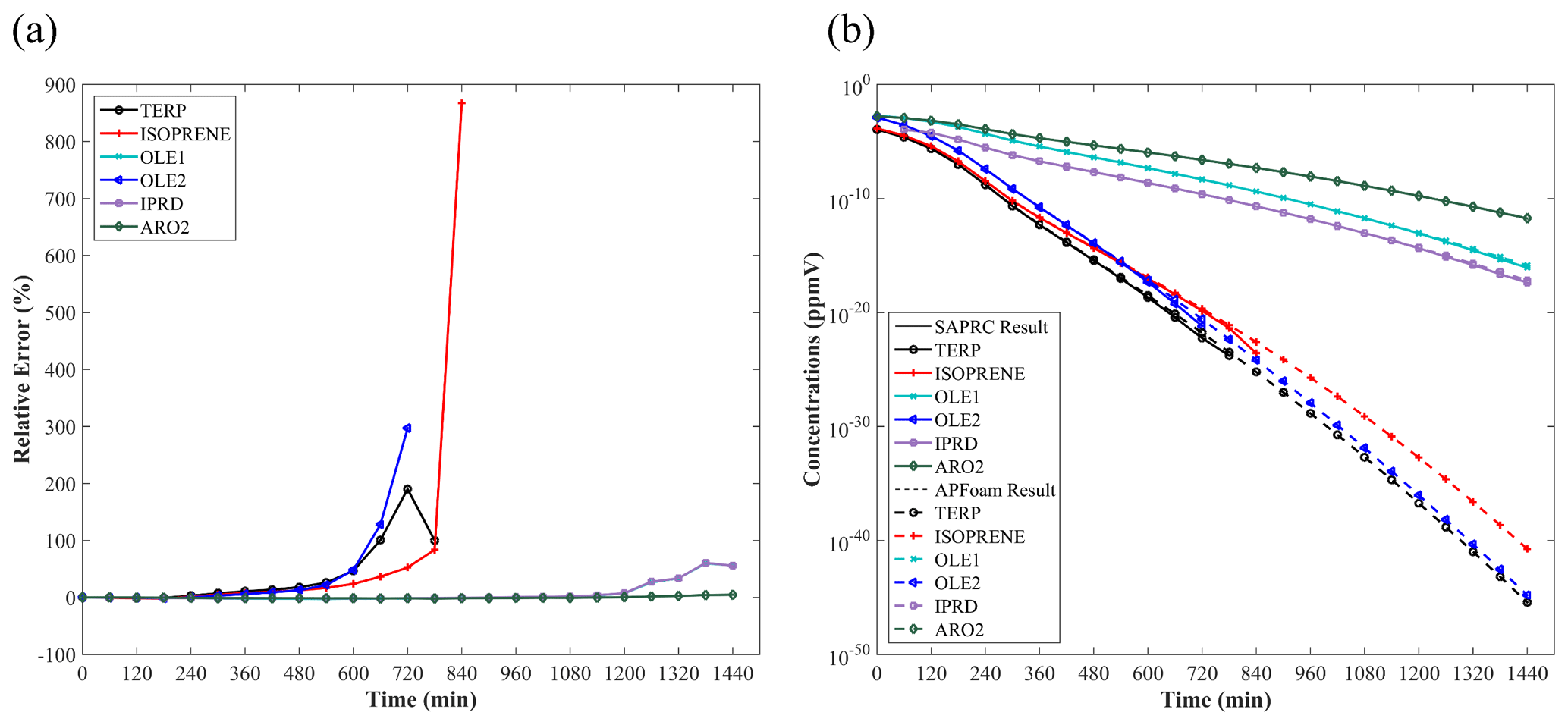
Figure 3The time series of (a) relative error (%) and (b) concentrations (ppmv) of the six species with largest bias.
Overall, most of the REi,t are less than 1 % in the concentration range between 0 to 10−20 ppmv (i.e., the concentrations under realistic conditions, ∼0 to 10−17 ppbv), indicating that the simulation error of APFoam is less than 1 % during the whole simulation period. However, there are six species with RE and MRE greater than 1 %: TERP, ISOPRENE, OLE1, OLE2, IPRD, and ARO2. The MRE of these six species are 44.0 %, 40.7 %, 7.74 %, 38.5 %, 7.71 %, and 1.20 %, respectively. Additionally, Fig. 3 shows time series of RE and concentrations for these high RE and MRE species. In Fig. 3a, RE values in the early stage of the simulation (t=0–180 min) are less than 1 % for these species. However, the REs of TERP, ISOPRENE, and OLE2 increase dramatically after t=180 min. The REs can even reach up to 190.4 %, 297.0 %, and 867.4 %, respectively, in the following simulation. It should be noted that at the later time the REs of these three species have no values because they are consumed during the chemical reaction and their concentrations from SARPC box model become zero. The significant increase in the RE values of OLE1 and IPRD begins at t=1020 min, with maximum RE values of 60.1 % and 60.9 %, respectively. Relatively, the RE of ARO2 is smaller, with a value of 5.0 %.
Figure 3b illustrates the concentration variation of these six species with the worst agreement from two models. It can be found that the concentrations of these six species keep dropping during the whole simulation period. Combined with the result of Fig. 3a, the dramatic increase of RE is due to the significant concentration decrease of these six species. In this study case, these six species are continuously consumed without supplement, which results in the concentrations of these species tending towards 0. For extremely small numbers, the processing of different model is diverse. Thus, when the reduction of magnitude exceeds 10−5 to 10−6 ppbv, the RE would become much larger between the two models. In the realistic situations, the concentrations of the species would not be completely consumed with continuous emission sources and boundary conditions. Therefore, the photochemical reaction simulation results of APFoam could be reliable, and the overall errors might be less than 1 %.
3.2 Numerical settings and validation studies in urban flow modeling
It is well known that large-eddy simulations (LES) perform more accurately when simulating urban turbulent characteristics than the Reynolds-averaged Navier–Stokes (RANS) simulations. However, RANS models (e.g., k-ε models) are still more widely utilized because of the disadvantages of LES, such as their much higher computational time and resource requirements, the difficulties in setting appropriate wall boundary conditions and defining the time-dependent domain inlet, and the challenges in developing advanced sub-grid-scale models. Among the RANS turbulence models, in contrast to the modified k-ε models (e.g., realizable and re-normalization group (RNG) k-ε models), although the standard k-ε model performs worse in predicting turbulence in the strong wind region of urban districts (e.g., separate flows near building corners), the prediction accuracy is better when simulating the low-wind-speed region (e.g., weak wind in a 2D street canyon sheltered by buildings at both sides) (Tominaga and Stathopoulos, 2013; Yoshie et al., 2007). Hence, as one of the widely adopted RANS methods, the standard k-ε model is selected to solve the incompressible steady-state turbulent flows in a 2D street canyon.
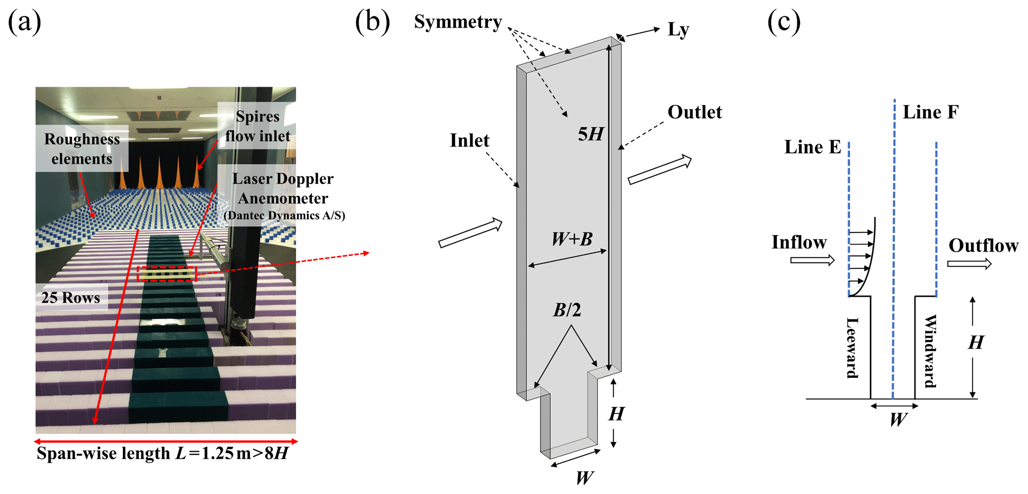
Figure 4(a) Wind tunnel experiment in a 2D street canyon. (b) The single street canyon CFD domain setups in the scaled model, (c) the inlet profile (Line E), and measurement profiles (Line F) in the street canyon.
To further evaluate the numerical accuracy of the turbulence flow simulation, a scaled CFD case is performed under the estimation of wind tunnel data. In the wind tunnel experiments (Fig. 4a), in total 25 rows of building models are set along the wind direction with the working section that is 11 m long, 3 m wide, and 1.5 m tall. For each row, building height (H), building width (B), and street width (W) are 12, 5, and 5 cm (i.e., aspect ratio ), respectively. The span-wise (or lateral) length is , which is sufficiently long to ensure the 2D flow characteristics in the street canyon (Hang et al., 2020; Oke, 1988; K. Zhang et al., 2019); i.e., the flow in the targeted street region is determined by the external flow above it but includes small impacts from the lateral boundaries. Free-flow wind speed in the wind tunnel experiment is 13 m s−1.
Figure 4b and c show the schematic diagrams of the CFD simulation domain setting for a single full-scale street canyon simulation. H and W of the street canyon are set as 24 and 10 m, with spatial scale ratio of 200:1 compared to the wind tunnel experiment. The corresponding Reynolds number () in the full-scale flow CFD validation (, H=24 m) is about 2.14×10⁷ and that in the wind-tunnel-scale experiments (, H=0.12 m) is 1.9×10⁵, which satisfies the requirement of Reynolds number independence (the critical level is about 8.7×10⁴ with the of 2) (Chew et al., 2018; Yang et al., 2020, 2021). The normalized wind profiles with two scales can be compared for validation purposes. Such validation techniques have been adopted in the literature (Hang et al., 2020; Yang et al., 2021). Besides, the building width B and Ly in the CFD simulation are 10 and 3.2 m (2), respectively, assuming that only a section () of long street canyons adopted with symmetry conditions is applied at two lateral boundaries. The minimum grid size in this case is 0.2 m, with an expansion ratio of 1.2 from the wall surface toward the around it, which refers to the grid independence tests from our previous research (K. Zhang et al., 2019). The upstream domain inlet profiles along Line E and comparison of profiles along Line F (Fig. 4c) are measured by the laser Doppler anemometry (LDA) system in wind tunnel tests. Additionally, CFD inlet profiles of stream-wise velocity (u) and turbulent kinetic energy (TKE) are fitted following the profiles in experimental data (Fig. 5).
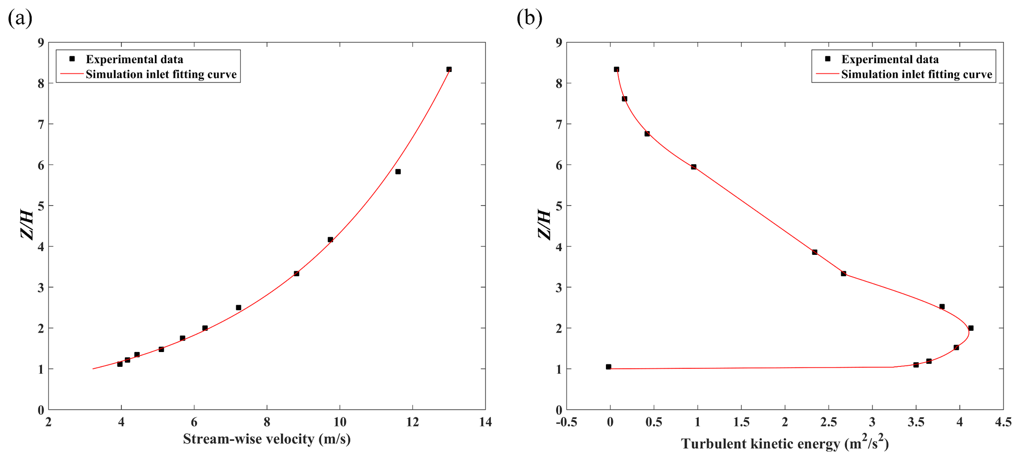
Figure 5The inlet profile of (a) stream-wise velocity and (b) turbulent kinetic energy in a single street canyon case.
All governing equations for the flow and turbulent quantities are discretized by FVM, and the SIMPLE scheme is used for the pressure and velocity coupling. The under-relaxation factors for the pressure term, momentum term, k term, and ε term are 0.3, 0.7, 0.8, and 0.8, respectively. CFD simulations do not stop until all residuals become constant. Typical residuals at convergence are , , and for Ux, Uy, and Uz, respectively; for continuity; for k; and for ε.
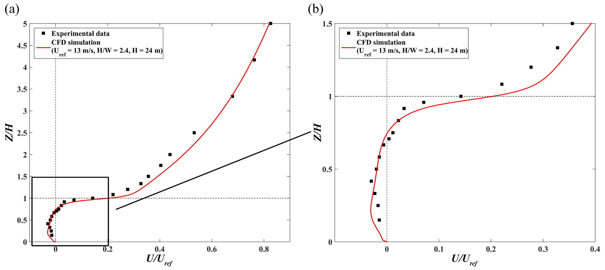
Figure 6 shows the stream-wise velocity profiles of simulation results and experimental data along the centerline (Line F) of the street canyon. The predicted wind profile agrees well with the wind tunnel data. One main vortex structure is formed in the street canyon. The center of the main velocity (i.e., where stream-wise velocity is 0) also matches well between simulation and experiment.
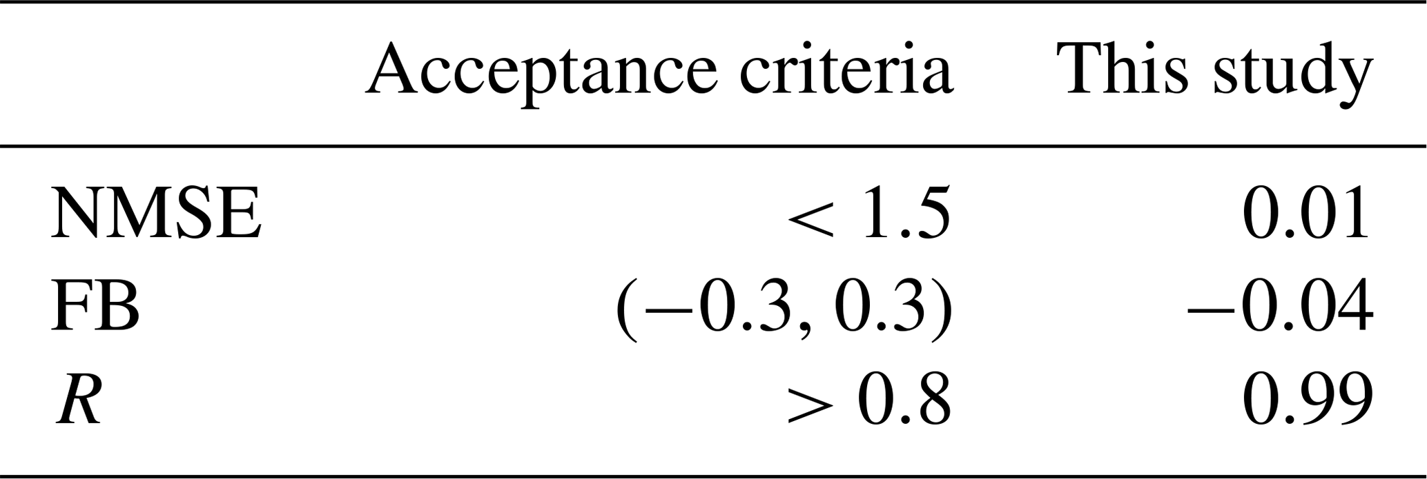
Furthermore, some statistical parameters, including normalized mean-square error (NMSE), fractional bias (FB), and correlation coefficient (R) are calculated by the following equations:
where n is the total number of measurement points, Oi is the experimental data at measurement point i, Pi is the CFD result at measurement point i, is the mean value of experimental data at all points, and is the mean value of CFD results at all points. According to the previous studies (Chang and Hanna, 2005; Sanchez et al., 2016), the model acceptance criteria for an urban configuration are NMSE < 1.5, , and R>0.8. In this simulation case, the respective NMSE, FB, and R are 0.01, −0.04, and 0.99, respectively (Table 2), which shows the good performance of APFoam in flow field simulation.
3.3 Pollutant dispersion in a 2D street canyon
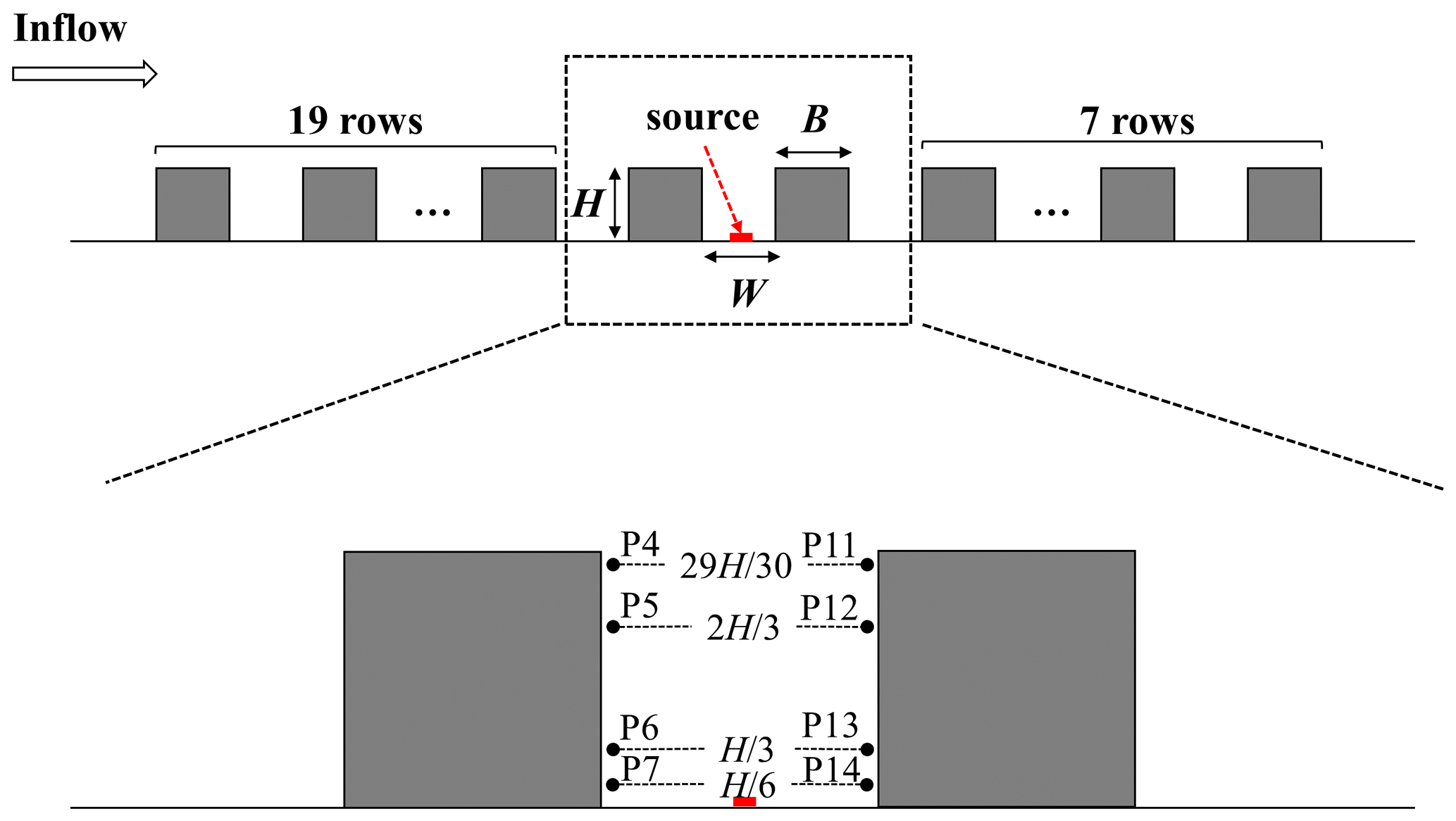
Currently, there are rarely wind tunnel experiments with chemical reactions. Thus, the pollutant dispersion accuracy in a 2D street canyon is validated by wind tunnel experimental data with tracer gas (Meroney et al., 1996), following previous studies (He et al., 2017; Zhang et al., 2020). The wind tunnel and the CFD domain configuration are presented in Fig. 7. A total of 28 rows of the wooden bar with 27 street canyons are set from upstream toward downstream along the inflow, and the street axis is perpendicular to the wind direction. Both the height (H) and width (B) of the bar are 0.06 m, and the street canyon width (W) is also 0.6 m, i.e., the aspect ratio () is 1 in this study case. A pollutant line source of ethane (C2H6) is set to emit the pollutant in the targeted street canyon. Following the wind tunnel configuration, there are 20 bars upstream and 8 bars downstream of the targeted street canyon. Eight measurement points are set in the targeted street canyon, with four (P4, P5, P6, P7) of them on the leeward side and the other four (P11, P12, P13, P14) on the windward side. The positions of the measurement points are demonstrated in Fig. 7. Pollutant concentrations at each measurement point are normalized with respect to that of the P7 (Ci/C7) within the street canyon (Sanchez et al., 2016; Santiago and Martín, 2008). For the CFD simulation, the APreactingFoam solver with the standard k-ε model is applied to solve the compressible unsteady-state turbulent flow field and pollutant dispersion. In order to be consistent with the wind tunnel experiment setting, the photochemical mechanism is not used in the simulation. The minimum grid size in this case is 0.5 mm, with an expansion ratio of 1.1 from the wall surface toward its surroundings, and the inlet velocity is constant at 3 m s−1 in the simulation. The time step of the simulation is set as s in this validation case.
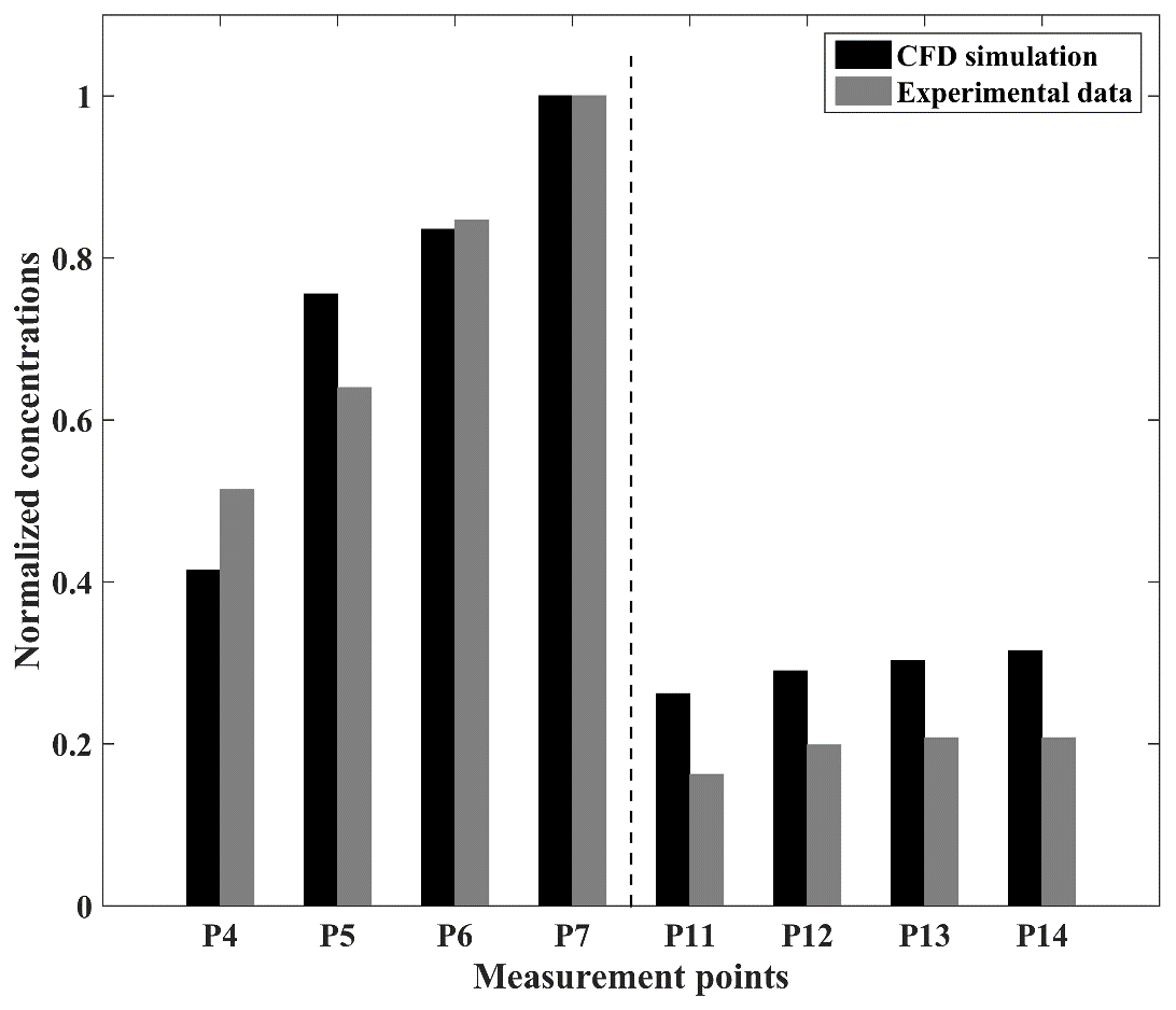
Figure 8Normalized concentrations of CFD and experimental data at each measurement point in the 2D dispersion case.
As a result of the comparison, Fig. 8 shows the normalized concentrations between the CFD simulation and experimental data. In general, the model slightly overestimates the C2H6 concentrations on the windward side. However, at P4 the model concentrations for the top of the leeward side are lower than the experimental data, and the simulation results at P5 overestimate the concentrations of the pollutants. In this simulation case, the respective values of NMSE, FB, and R are 0.06, −0.13, and 0.95 (Table 3), which shows the good performance of APFoam in 2D pollutant dispersion simulation.
Table 3Static values of the 2D pollutant dispersion simulation.
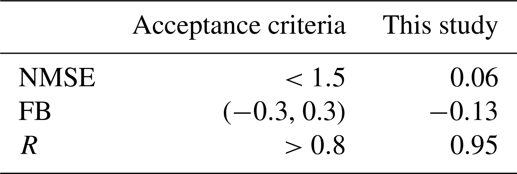
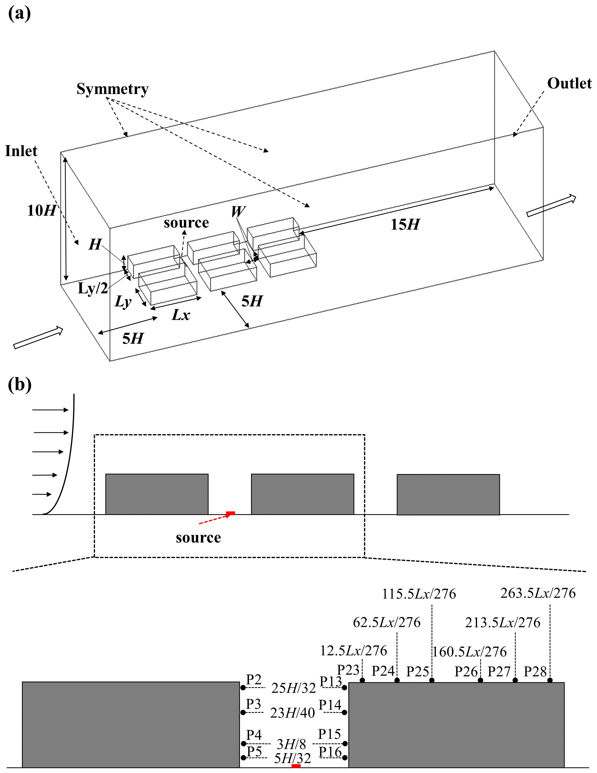
Figure 9(a) The simulation domain of 3D pollutant dispersion and (b) the measurement points' locations in the street canyon.
3.4 Pollutant dispersion in a 3D street canyon
As mentioned in Sect. 3.3, 3D pollutant dispersion validation with tracer gas is conducted in this study, following the previous study (Y. Zhang et al., 2019). Simulation results are also compared with the wind tunnel experimental data (Chang and Meroney, 2001). The CFD domain configuration is presented in Fig. 9a. In this case, six buildings are set in the domain. Building height (H) and street canyon width (W) are both 0.08 m with . Building length (Lx) and building width (Ly) are 0.276 and 0.184 m, respectively. The distance between the buildings and the domain inlet, side boundary, top boundary, and domain outlet is 5H, 5H, 10H and 15H, respectively, for simulating realistic results (Tominaga et al., 2008). Within the target street canyon, there are also eight measurement points (four are on the leeward side, and four are on the windward side) for measuring the concentrations (Fig. 9b). In addition, six more measurement points are also set on the top of the downstream building. Pollutant concentrations at each measurement point in this simulation case are normalized with respect to the P5 (Ci/C5) within the street canyon. The source of the C2H6 is set as an inlet at the bottom of the target street canyon. The size of the source is 0.005 m in width and 0.092 m in length, and it is set in the middle of canyon. The release velocity is 0.01 m s−1 toward the top boundary and the mass fraction of the C2H6 is 1 (pure gas of C2H6). For the 3D pollutant dispersion simulation, an APreactingFoam solver with a standard k-ε model is applied to solver-compressible unsteady-state turbulent flow and pollutant dispersion. The photochemical mechanism is not used in the simulation. The minimum grid size in this case is 0.0005 m with an expansion ratio of 1.1 from the wall surface toward the surrounding area. The time step of the simulation is set as s in this validation case as well. Meanwhile, the inlet velocity and TKE profile are also retrieved from and fitted by the experimental data (Fig. 10).
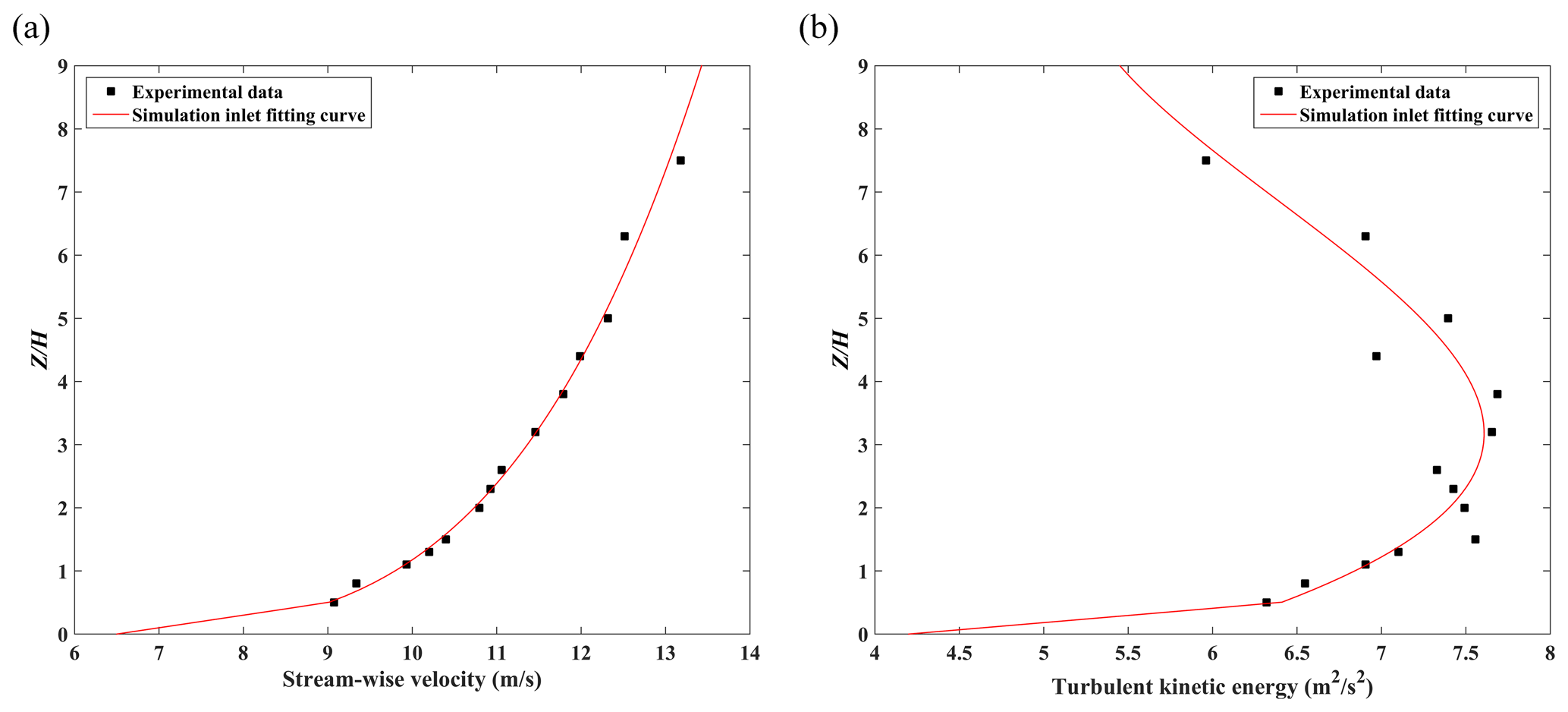
Figure 10The inlet profile of (a) stream-wise velocity and (b) turbulent kinetic energy in the 3D dispersion case.

Figure 11Normalized concentrations of CFD and experimental data at each measurement point in the 3D dispersion case.
Figure 11 shows the comparison results between the CFD simulation and experimental data. Overall, the CFD simulation in the 3D dispersion case slightly overestimates the concentrations in the street canyon. As for P23 and P24, the simulated results also overestimate the concentrations, as they are affected by the higher concentrations predicted within the street canyon. Similarly, statistical variables such as NMSE, FB, and R are calculated to evaluate the performance of the model. As shown in Table 4, the value of NMSE, FB, and R is 0.16, −0.21, and 0.93 in the 3D dispersion case, respectively, which agrees with the acceptance criteria. In general, APFoam also shows the good performance of the 3D pollutant dispersion simulation.
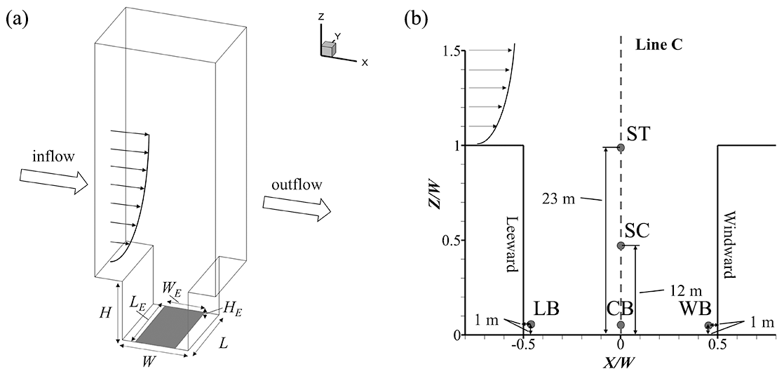
Figure 12Schematic diagram of (a) the CFD simulation domain and (b) the probe point locations.
Table 4Static values of the 3D pollutant dispersion simulation.

4.1 Simulation configuration and CFD setting
In this study, APFoam with a CS07A photochemical mechanism is applied for the street air quality simulation. As shown in Fig. 12a, the street aspect ratio () is set with building height (H=24 m), street width (W=24 m), and span-wise street length (L=30 m). A telescoping multigrid approach is adopted in the simulation with a minimum grid size of 0.2 m and an expansion ratio of 1.2 from the building walls to the surrounding area. The total grid number is about 87 300 for the whole CFD domain. The top and two lateral boundaries of the domain are set up as the symmetry boundary conditions. The emissions area is set up at the bottom of street canyon with a pollutant source size of 18 m (width, WE) × 30 m (length, LE) × 0.3 m (height, HE), representing traffic emissions near street level, and emissions data are obtained from our previous work (Wu et al., 2020). In this study, the emissions of NOx, VOCs, and CO are , , and kg m−3 s−1 (i.e., ∼35, ∼200, and ∼170 ppbv s−1), respectively. The NO and NO2 are separated from NOx by a ratio of 9:1, which is similar to the previous study (Baik et al., 2007). VOCs are speciated following the SAPRC mechanism, and the emission fraction of the species is obtained from the literature (Carter, 2015).
Figure 12b shows the probe point locations for the numerical case, wherein temporal variations of reactive pollutant concentrations are monitored, which include three points at a pedestrian height of z=1 m (near the street bottom at the leeward side (LB), center (CB), and windward side (WB)) and two other probe points near the street top (ST, z=23 m) and street center (SC, z=12 m = 0.5H).
A power-law velocity vertical profile is adopted for the inflow boundary condition, which is described as follows:
Here the reference velocity Uref is 3 m s−1, the reference height zref is 24 m, the turbulence intensity Iin is 0.1, the power-law exponent α is 0.22 (He et al., 2017; K. Zhang et al., 2019, 2020), the Von Kármán constant κ is 0.41, and the Cμ is 0.09.
In addition, the initial and inlet background concentrations for O3, NO, NO2, VOCs, and CO are 60, 5, 15, 40, and 400 ppbv, respectively, which are obtained from an observation campaign (Liu et al., 2008). For meteorological conditions, the temperature is 300 K and the operating pressure is 1013.25 hPa.
In all simulation cases, the steady-state turbulence field is first solved in advance. The result of turbulent flow drives the chemistry solution from t=0. During t=0–30 min (1800 s), the emission and chemistry solution are turned on under the statistically steady turbulent flow, reaching a quasi-dynamic and photostationary steady state. Data from the next 60 min (t=30–90 min, 1800–5400 s) are used for analysis. The time step of the chemistry solution is set as 0.1 s in all numerical cases.
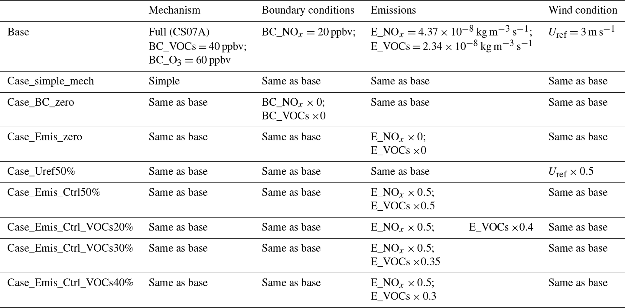
A description of all simulation cases is given in Table 5. All CFD simulations are finished with the Tianhe II supercomputer and supported by National Supercomputer Center in Guangzhou. To investigate the effect of the chemical mechanism, the background condition of the precursors (BC), emissions (Emis), and wind conditions (Uref) of the reactive pollutant concentrations in the street canyon, the cases of BC_zero_out, Emis_zero_out, and Uref0.5 are set up in numerical simulations. In Case_BC_zero and Case_Emis_zero, the precursors of O3 (i.e., NOx and VOCs) are removed from the domain inlet (background boundary conditions) and pollutant source emissions, respectively, and then we compare the results with the base case. In Case_Uref50%, the Uref is reduced by 50 % to investigate the contribution of wind conditions to the chemical reaction. However, in Case_simple_mech, only three photochemical reactions (Leighton, 1961) are considered in the simulation.
In order to improve the air quality within the urban area, some cities have tried to implement traffic control policies to reduce the pollutants from vehicle emission sources. Thus, four emission control scenarios are carried out to investigate the effect of emission reduction. Case_Emis_Ctrl50% is the scenario where 50 % of the traffic volume is reduced by applying the odd–even license plate policy (i.e., reducing 50 % of the total vehicle emissions). Case_Emis_Ctrl_VOC20%, Case_Emis_Ctrl_VOC30%, and Case_Emis_Ctrl_VOC40% are the scenarios that apply the stricter VOC control measures (corresponding to 20 %, 30 %, and 40 % more VOC emission reduction, which is a 60 %, 65 %, and 70 % reduction of total VOC emission, respectively) on the vehicles using traffic control policies.
Additionally, the change rate is used to reveal the effect of different factors on pollutant concentrations in the street canyon. For each pollutant, the change rate (CRp) for different cases is defined as
where Ccase and Cbase are the concentrations regarded as the condition change case and base case, respectively.
4.2 The comparison of pollutant distribution among the 3D CFD solvers
To investigate the difference between the APonlyChemReactingFoam, APreactingFoam, and APSteadyReactingFoam results, comparisons of O3, NO, NO2, and CO distribution are conducted in a street canyon in this study. For APonlyChemReactingFoam, the flow field is treated as the incompressible steady-state flow and pre-solved using the SIMPLE method. The under-relaxation factors and residual threshold for convergence are the same as the setting in Sect. 3.2. Chemical reaction and pollutant dispersion are solved under the steady-state flow for 90 min. For the APreactingFoam and APSteadyReactingFoam cases, turbulence flow, chemical reaction, and pollutant dispersion are solved simultaneously for 90 min. The results in Fig. 13 and all subsequent figures are the pollutant dispersion at 90 min.
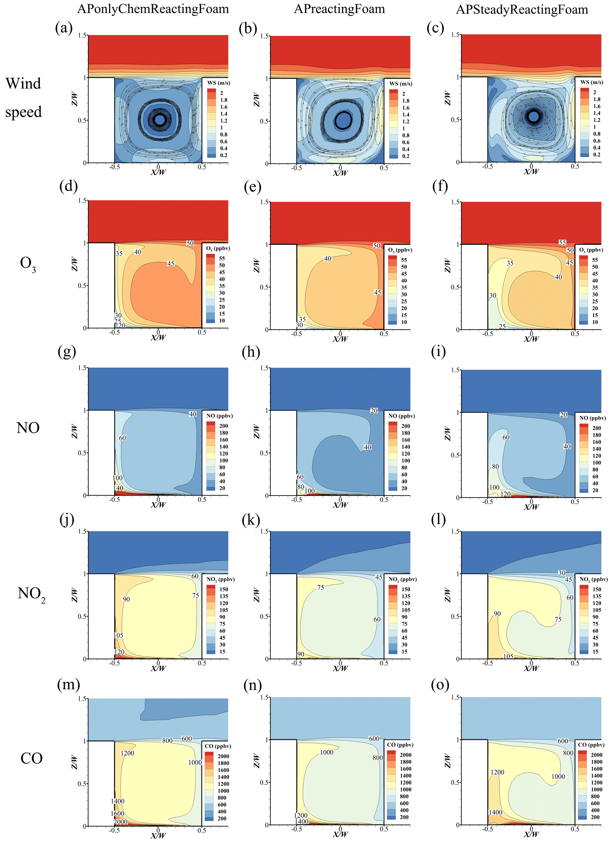
Figure 13The comparison of (a–c) wind speed, (d–f) O3, (g–i) NO, (j–l) NO2, and (m–o) CO between APonlyChemReactingFoam, APreactingFoam, and APSteadyReactingFoam.
As depicted in Fig. 13, the wind speed in the APonlyChemReactingFoam case (Fig. 13a) is lower than that in the APreactingFoam (Fig. 13b) and the APSteadyReactingFoam (Fig. 13c) cases. The reason for the difference is most likely due to the different turbulence flow algorithm, where the turbulence is treated as incompressible steady flow, compressible unsteady flow, and compressible steady flow in APonlyChemReactingFoam, APreactingFoam, and APSteadyReactingFoam, respectively. Because of the slight difference in wind speed, the concentrations of APonlyChemReactingFoam (Fig. 13d, g, j, m) for pollutants are higher (due to the lower wind speed) than those in the APreactingFoam (Fig. 13e, h, k, n) and APSteadyReactingFoam (Fig. 13f, i, l, o) cases.

Table 6 shows the elapsed time of these three simulations in same street canyon for the 90 min simulation. In total, the elapsed time of the APonlyChemReactingFoam case (226 min) is slightly longer than that of the APreactingFoam (214 min) and APSteadyReactingFoam (217 min) cases when employing 192 CPU cores (16× Intel® Xeon® E5-2692) for the simulation. However, if the flow field has been determined and there is no need to recalculate in the simulation case, the APonlyChemReactingFoam only takes 191 min to solve the chemical reaction and pollutant dispersion, which is 11 % less time than APreactingFoam.
Many previous studies have treated the urban air turbulence as incompressible steady-state flow and investigate the pollutant dispersion successfully (He et al., 2017; Ng and Chau, 2014; K. Zhang et al., 2019, 2020; Y. Zhang et al., 2019). The APonlyChemReactingFoam is applied in the study over a shorter period of time to analyze the photochemical reaction process in the street canyon.
4.3 Pollutant concentration distribution with a full chemistry mechanism vs. simple chemistry
As shown in Fig. 13a, one main clockwise vortex is formed in the street canyon with . The wind speed (WS) is small near the vortex center; i.e., the minimum wind speed is approximated at 0.03 m s−1, which is only 1 % of the speed at the domain inlet. The distributions of pollutants in the street canyon, such as O3, NO, and NO2, are also swirling (Fig. 13a, d, g, j).
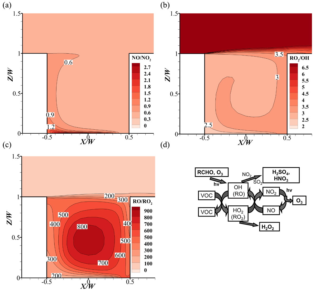
Figure 14Pollutant distribution of (a) , (b) , and (c) in the base case. (d) Schematic diagram of the formation mechanism of photochemical reactions (Tang et al., 2006).
Leeward-side O3 concentration in the base case is less than the windward side, while NO and NO2 are the opposite. At the corner of leeward side, the minimum value of O3 and maximum value of NOx appear, with less than 20 ppbv for O3, more than 200 ppbv for NO and 140 ppbv for NO2 (Fig. 13a, d, g, j), respectively. Meanwhile, due to the higher NO emissions, the ratios of NO and NO2 are higher at the bottom of the street canyon (Fig. 14a). The larger values indicate that the titration effect from NO () and ozone depletion would be stronger, leading to the lower O3 concentrations in this area.
However, on the windward side, NOx concentrations are less than that on the leeward side. This is because the NOx from the emission source first affects the leeward side, which leads to the high concentrations in this area. As the wind flows, the concentrations of NOx gradually decrease due to the wind diffusion and the dilution effect. With the comparison of background, the windward NO and NO2 concentrations increase by approximately 35 and 55 ppbv, respectively. On the one hand, pollutants from emissions are transported along the flow, which increases the concentrations. On the other hand, VOCs in street canyons react with OH via the chemical reactions and generate HO2 and RO2. Theis RO2, HO2, and O3 would react with NO and generate NO2, leading a higher increment for NO2 (Fig. 14b–c). It should be noted that the O3 concentrations could be higher due to the lower depletion reaction with NO compared to that of the leeward side.
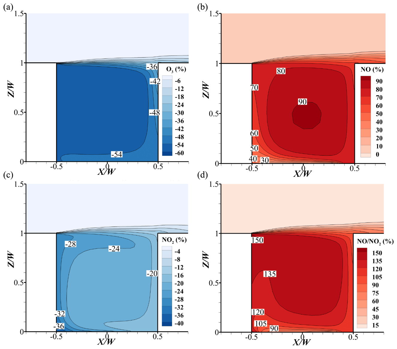
Figure 15Change rate of (a) O3, (b) NO, (c) NO2, and (d) between the simple chemistry and full chemistry mechanisms.
Figure 15 shows the change rate of pollutant concentrations (Fig. 15a–c) and the NO to NO2 ratio change rate of Case_simple_mech compared with the base case (Fig. 15d). Without the consideration of the VOC-related reactions in the mechanism, there is no consumption of NO by RO2 in the mechanism (, ), and the NO titration effect () would be stronger in this case. For O3, the concentrations are 36 %–58 % lower than that in base case within the street canyon; NO2 concentrations are also 15 %–40 % lower, and NO could be up to 90 % higher than that in the simple chemistry case. Thus, the NO to NO2 ratio would be 60 %–150 % higher in the simple chemistry case.

Figure 16Change rate of (a) O3, (b) NO, (c) NO2, (d) , (e) , and (f) at t=5400 s .(g) Time series of the reaction rate of RO2 () of Case_BC_zero.
4.4 Influence of background precursors of O3 on reactive pollutant concentrations
In Case_BC_zero, all background precursors of O3 (i.e., NOx and VOCs) from the upstream domain inlet are removed. As depicted in Fig. 16a, the change rates of O3 are negative, confirming that O3 concentration becomes lower without the background NOx and VOCs. In addition, the O3 reduction rate on the windward side (−5 % to −8 %) is smaller than that on the leeward side (−9 %). The influencing mechanisms of O3 reduction are complicated and will be explained later.
On the one hand, by analyzing Fig. 16b and c, such reduction rates on the windward side for NO (−12 % to −16 %) and NO2 (−20 % to −24 %) are greater than those on the leeward side (−2 % to −6 % for NO and −12 % to −15 % for NO2). Therefore, the ratio of increases from about 9 % to 14 % in the street canyon (Fig. 16d). Overall, this increment of enhances O3 depletion because the main source of ozone is the photolysis reaction of NO2. Meanwhile, the main sink is the titration effect of O3 and NO.
On the other hand, the RO2 from the oxidation of VOCs with OH will consume the NO (, ), which would affect the NOx–O3 circulation. Figure 16e shows that the reduction of on the windward side is more than that on the leeward side, which indicates that the background VOCs and OH reaction on the windward side are more active. However, due to the slower reaction rate of RO2 and NO compared to that of HO2 and O3 with NO, the conversion of RO2 to RO by reacting with NO would require more time. The reduction rate of (Fig. 16f) on the leeward side (−18 % to −23 %) is slightly greater than that on the windward side (−16 % to −17 %). Therefore, the influence of RO2 on NOx–O3 circulation would gradually appear on the leeward side, in addition to the flow transportation.
Additionally, Fig. 16g shows the reaction rate of RO2 () at the bottom, center, and top point on the centerline of the street canyon with (base) and without (Case_BC_zero) background conditions. At the bottom point (CB), the reduction rate of RO2 is lower in the base case. This is because the background VOCs and OH reaction consume a portion of NO on the windward side, which leads to a lower consumption of RO2 with NO. As the simulation continues, NO concentrations would increase due to the continuous release of large amounts of NO from source emissions, and the reduction rate of RO2 becomes lower in Case_BC_zero due to the lack of background VOCs.
At the top (ST) and center point (SC), however, as the reaction goes on and pollutants mix upwards, the NO concentration could become higher. Therefore, the RO2 consumption rate is lower without the background RO2. This reduction indicates that the background conditions mainly consume NO in the street canyon, which leads to the increase of O3 due to the weakening titration effect.
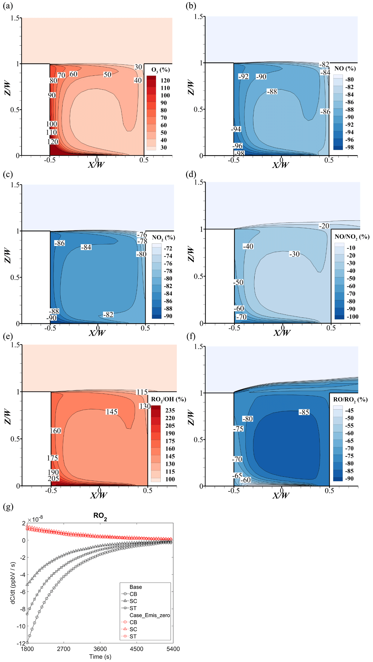
Figure 17Change rate of (a) O3, (b) NO, (c) NO2, (d) , (e) , and (f) at t=5400 s. (g) Time series of the reaction rate of RO2 () of Case_Emis_zero.
4.5 Effects of vehicular source emissions on reactive pollutants
In Case_Emis_zero, the precursors of O3 (NOx and VOCs) from near-ground emissions are removed. As shown in Fig. 17a, O3 concentrations increase by over 30 %–120 % in the whole street canyon compared to the base case. In particular, the O3 increment on the leeward side is from 80 % to 250 % (not shown here), which is much higher than that on the windward side (30 % to 40 %). However, NOx concentrations decrease significantly, i.e., the reduction rates are −84 % to −98 % for NO and −76 % to −90 % for NO2, showing that the NOx from source emissions is the dominant part of NOx in the street canyon (Fig. 17b and c). The large reduction of NOx concentrations induces the increase of O3 concentrations with weaker titration effect of O3. Specifically, both the maximum increase for O3 and minimum reduction of NO and NO2 appear at the near-ground corner of the leeward side, which is the downwind area of the pollutant source. In addition, due to a larger amount of NO emissions than NO2 (emission ratio of NO to NO2 is 9:1), the concentration ratio of considerably decreases with the reduction rates of −30 % to −70 % (Fig. 17d) if vehicular pollutant sources are removed.
Additionally, due to the large reduction of NO and NO2 concentrations, more OH would react with VOCs instead of NOx, which increases the RO2 concentration (Fig. 17e and f). Meanwhile, with the reduction of NO concentration, the consumption of RO2 significantly decreases, which leads to the dramatic increase of RO2 concentration. Thus, the ratio of rises by 115 %–205 % and the ratio of decreases by −60 % to −88 %.
In Fig. 17g, the reaction rate of RO2 at three points in Case_Emis_zero is positive, which means that the RO2 keeps being generated but is not consumed among these three points. As mentioned above, RO2 (the production of VOCs and OH) will consume the NO and weaken the O3 titration effect with NO. In the base case (Fig. 17g), the reaction rate of RO2 is negative, which means that RO2 consumes the NO. However, in Case_Emis_zero, the reaction rate of RO2 is positive during the whole simulation period, which means that there is not enough NO to react with RO2 or even O3 without the vehicular source. Therefore, the source emissions provide a large amount of NO, which enhances the O3 depletion in the street canyon.
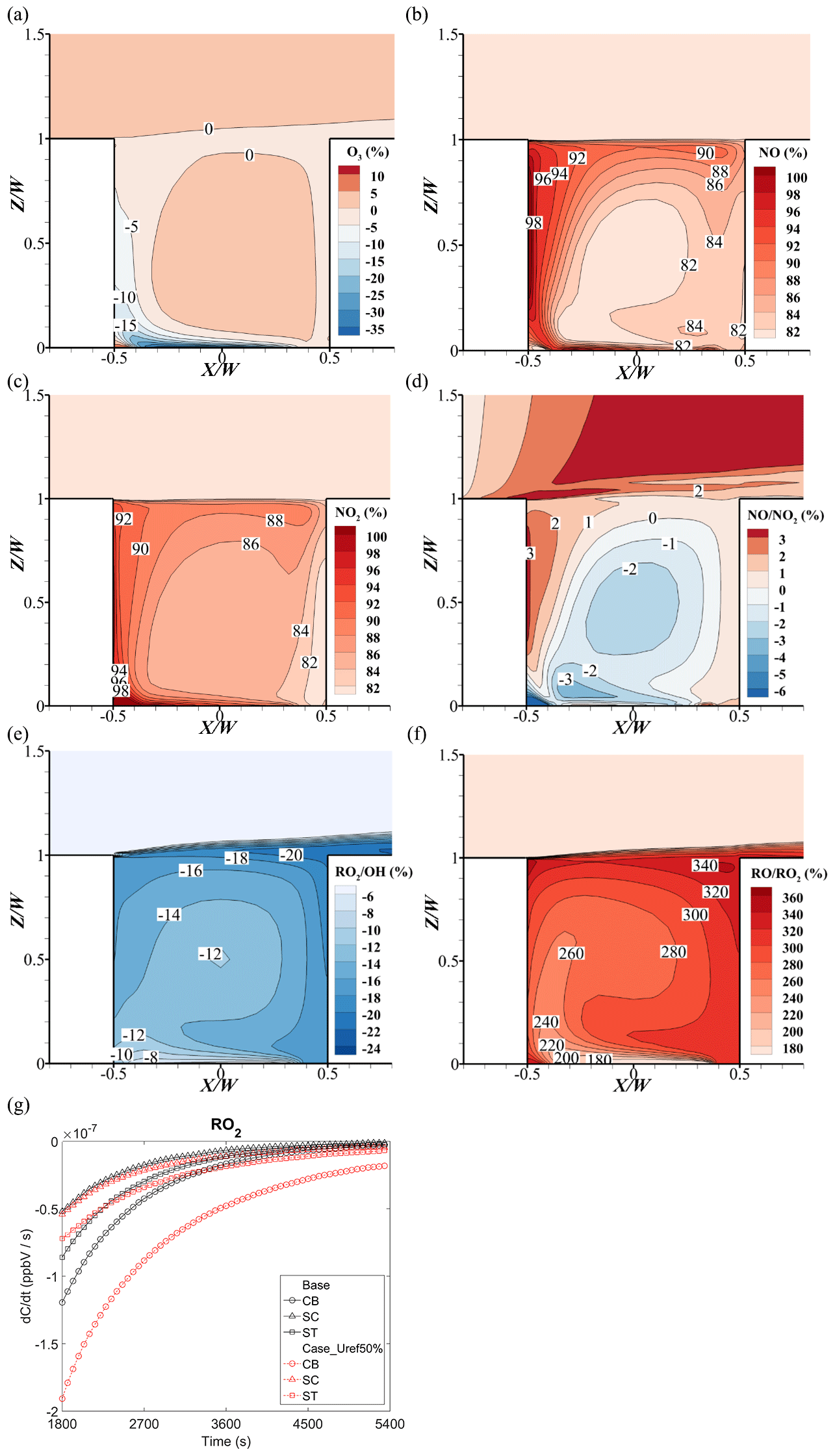
Figure 18Change rate of (a) O3, (b) NO, (c) NO2, (d) , (e) , and (f) at t=5400 s.(g) Time series of the reaction rate of RO2 () of Case_Uref50%.
4.6 Influence of wind velocity reduction on reactive pollutants
Figure 18 shows the change rates of O3, NOx, and ratios when the background wind speed decreases from Uref=3 m s−1 (base) to Uref=1.5 m s−1 (Case_Uref50%). In Fig. 18a, there is no significant change of O3 concentration at the center of street canyon. However, in the downwind area of the near-ground pollutant source, O3 concentration decreases by 5 % to 30 % compared with that of the base case. Interestingly, at the bottom of the leeward side, O3 has an increase up to 6 % under the half inlet wind speed condition.
Due to the weaker capacity of pollutant dilution caused by the smaller wind speed, the concentrations of NO and NO2 almost double (i.e., rising by 80 %–98 % in Fig. 18b and c), but the change rate has no significant change (−1 % to −3 % in Fig. 18d). Besides, a higher NOx concentration would react with more OH, which consequently weakens the RO2 production from VOCs (−8 % to −20 % in Fig. 18e). Meanwhile, the increase of NO concentration consumes more RO2 to RO, which leads to an 180 % to 340 % increase of (Fig. 18f).
Additionally, Fig. 18g illustrates the RO2 reduction in a street canyon. Because of the higher concentration of NO in Case_Uref50%, the RO2 reduction rates at three monitoring points are higher than that in the base case, particularly at the bottom of the street canyon (CB). In the early stages of the reaction, the reduction rate of RO2 at the top point (ST) is slightly lower in Case_Uref50%. This is because the RO2 concentration at ST is first affected by the background. As the NO concentrations increase in the whole street canyon, the RO2 consumptions become higher than that in the base case.
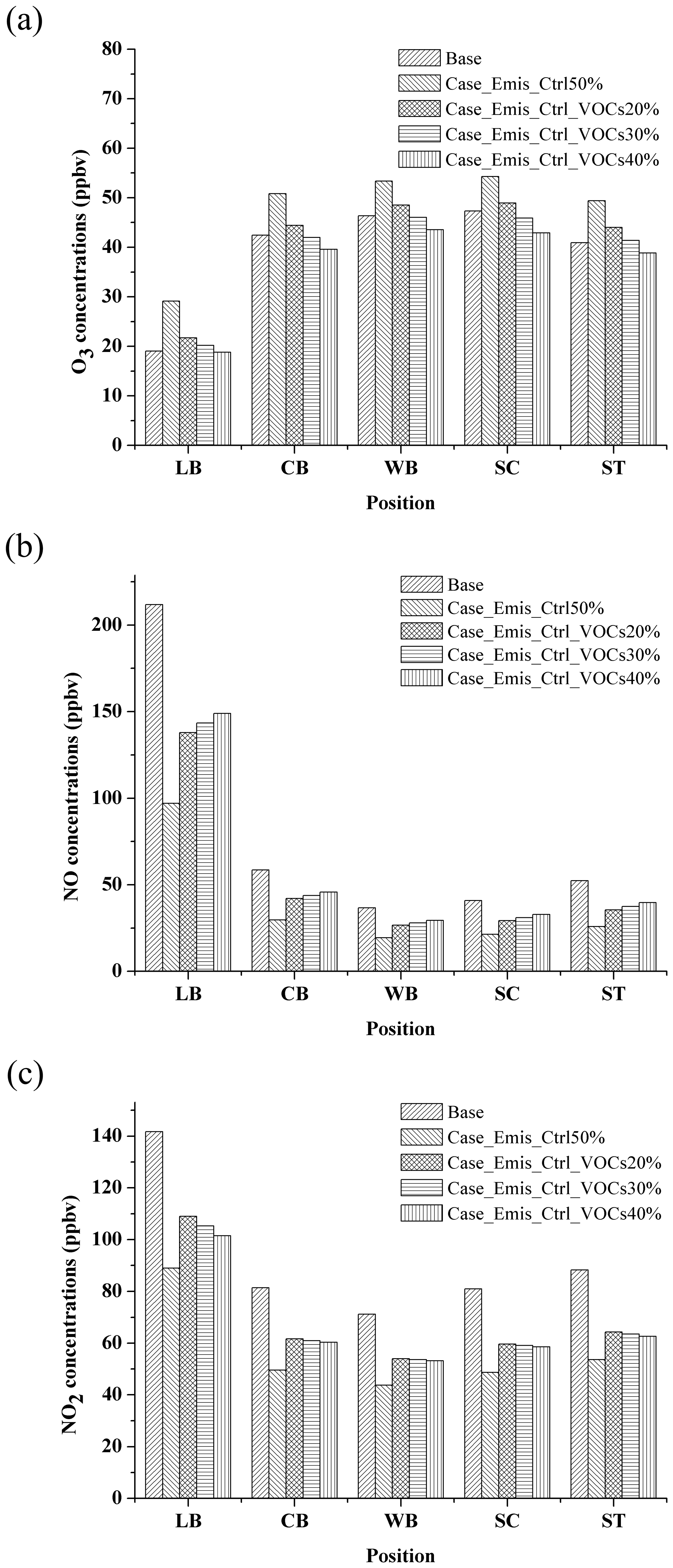
Figure 19The (a) O3, (b) NO, and (c) NO2 concentrations at 90 min in different emission control scenarios.
4.7 Emission control strategy on reactive pollutant concentrations
Figure 19 shows the concentrations of O3, NO, and NO2 in different NOx and VOC emission control scenarios at 90 min. In Case_Emis_ctrl50% (the emission of NOx and VOCs reduces 50 %, i.e., 50 % reduction of traffic volume), the O3 concentration increases from 19–47 to 29–54 ppbv (Fig. 19a). On the contrary, this control measure for NO and NO2 is very effective (Fig. 19b and c), and NO and NO2 concentrations reduce from 47 % to 54 % and 37 % to 40 % in Case_Emis_ctrl50%, respectively.
This indicates that the simple traffic control measures cannot effectively reduce O3 concentration. This is because most of the urban areas are in VOC-sensitive regions (Ye et al., 2016). When the total number of vehicles decreases under the traffic control measures, the reduction of NOx is higher than that of the VOCs (due to the larger NOx emission from vehicles), which leads to a higher VOC-to-NOx ratio, consequently resulting in a higher O3 concentration in the street canyon (Sillman and He, 2002). Thus, in order to reduce the concentrations of O3, the stricter VOC control measures on vehicles should be conducted. Based on the results shown from three other emission control scenarios (Case_Emis_ctrl_VOCs20%, Case_Emis_ctrl_VOCs30% and Case_Emis_ctrl_VOCs40%) in Fig. 19a, the emission of VOCs needs be reduced by another 30 % under traffic control (Case_Emis_ctrl50%) to bring the O3 concentrations back to the level that they were at when no traffic control measures had been taken (base case).
As for NO and NO2, when the additional VOC control measures are carried out, the concentrations are higher than those in Case_Emis_ctrl50%. Even so, their concentrations do not still exceed the concentration level before the traffic control (base case), which means that such an emission control scenario is still effective for NO and NO2. In summary, the control policies of reactive pollutants require the comprehensive consideration of the relationship between precursors and pollutants so that the goal of improving air quality can be achieved.
A detailed description of the atmospheric photolysis calculation framework APFoam 1.0 is presented in this paper, and this CFD model is coupled with multiple full atmospheric photochemical mechanisms, including SAPRC07 (CS07A and SAPRC07TB) and CB05. In order to simulate the photochemical process of reactive pollutants, five new types of the reactions, i.e., the new form of the (1) Arrhenius reactions, (2) photolysis reactions, (3) falloff reactions, (4) “three-k” reactions, and (5) “two-k” reactions, have been modified and added into APFoam. Additionally, to verify the model performance, several validations, including a photochemical mechanism (CS07A) with SAPRC box modeling, a flow field, and 2D and 3D pollutant dispersions with wind tunnel experimental data have been conducted in this study. The model results show a good agreement with the SAPRC box modeling and wind tunnel experimental data, indicating that APFoam can be applied in the analysis of microscale urban pollutant dispersion.
Key factors of chemical processes are investigated by applying APFoam with a CS07A mechanism in the simulation of reactive pollutants in a typical street canyon () with a VOC to NOx emission ratio of ∼5.7 ppbv s−1. In the comparison of chemical mechanisms, O3 and NO2 are underestimated by 36 %–58 % and 15 %–40 %, respectively, while NO is overestimated by 30 %–90 % without the consideration of the VOC reactions. Other numerical sensitivity cases (Case_BC_zero, Case_Emis_zero, and Case_Uref50%) reveal that vehicle emissions are the main source of NO and NO2, with a contribution of 82 %–98 % and 75 %–90 %, respectively. The resident part of the NOx in the street canyon is contributed by the background concentration. However, vehicle emissions with a large amount of emitted NOx, especially NO, are the main reason for the decrease of O3 due to the stronger NO titration effect within the street canyon. In contrast, 5 %–9 % of the O3 is contributed by the boundary conditions. Ventilation conditions are another reason for the NOx concentration increments, and the increase of NOx can be up to 98 % when the wind speed is reduced by half. If there are no chemical reactions, NOx concentration should rise by 100 % when the wind velocity decreases by 50 % (i.e., ventilation capacity reduces by 50 %) because the Re independence requirement is satisfied. However, O3 is reduced downwind of the emissions due to the increase of NO concentrations. In order to control and improve the air quality in the street canyon, traffic control policies are effective for NOx. However, our results indicate that at least another 30 % reduction in vehicle VOC emissions could reduce O3 concentrations below those of the odd–even license plate policy, with 24 %–32 %, 25 %–28 %, and −6 %–2 % reduction rates of NO, NO2, and O3, respectively. Overall, APFoam 1.0, a fully coupled CFD model, can be employed to investigate atmospheric photolysis calculation in urban areas and provide reliable and useful suggestions for the improvement of urban air quality.
However, in the current version of APFoam, aerosol chemistry is not included in the model, and thus it is necessary to couple it with aerosol processes, such as MOSAIC (Zaveri et al., 2008) or ISORROPIA (Fountoukis and Nenes, 2007; Nenes et al., 1998), in future work. In addition, the photolysis rates in the current model have been fixed without diurnal variation, which means that the model is not suitable for a long-term simulation and needs to be updated in subsequent versions. Moreover, the interaction between radiation and chemical reactions will be investigated by APFoam and validated by the scaled outdoor experiment (Chen et al., 2020a, b) in the future.
The source code of the APFoam 1.0 model and examples of its use are available on GitHub (https://github.com/vnuni23/APFoam, last access: 18 November 2020) and Zenodo (https://doi.org/10.5281/zenodo.4279172, Wu, 2020). More information and help are also available by contacting the authors.
The data are included in the tutorial cases of the model, which are available on GitHub (https://github.com/vnuni23/APFoam, last access: 18 November 2020) and Zenodo (https://doi.org/10.5281/zenodo.4279172, Wu, 2020).
LW and XW designed the experiments. LW and CG developed the model code. LW and JH performed the simulations and organized the results of model cases. LW and JH prepared the article with contributions from all co-authors. XW and MS proposed revision suggestions for the article.
The authors declare that they have no conflict of interest.
We acknowledge the technical support and computational time from the Tianhe II platform at the National Supercomputer Center in Guangzhou and the support from Collaborative Innovation Center of Climate Change, Jiangsu province, China.
This research has been supported by the National Key Research and Development Program of China (grant no. 2016YFC0202206) and the National Nature Science Fund for Distinguished Young Scholars (grant no. 41425020).
This paper was edited by Christoph Knote and reviewed by two anonymous referees.
Atkinson, R., Baulch, D. L., Cox, R. A., Crowley, J. N., Hampson, R. F., Hynes, R. G., Jenkin, M. E., Rossi, M. J., and Troe, J.: Evaluated kinetic and photochemical data for atmospheric chemistry: Volume I – gas phase reactions of Ox, HOx, NOx and SOx species, Atmos. Chem. Phys., 4, 1461–1738, https://doi.org/10.5194/acp-4-1461-2004, 2004.
Baik, J. J., Kang, Y. S., and Kim, J. J.: Modeling reactive pollutant dispersion in an urban street canyon, Atmos. Environ., 41, 934–949, https://doi.org/10.1016/j.atmosenv.2006.09.018, 2007.
Baker, J., Walker, H. L., and Cai, X.: A study of the dispersion and transport of reactive pollutants in and above street canyons – A large eddy simulation, Atmos. Environ., 38, 6883–6892, https://doi.org/10.1016/j.atmosenv.2004.08.051, 2004.
Bright, V. B., Bloss, W. J., and Cai, X.: Urban street canyons: Coupling dynamics, chemistry and within-canyon chemical processing of emissions, Atmos. Environ., 68, 127–142, https://doi.org/10.1016/j.atmosenv.2012.10.056, 2013.
Britter, R. E. and Hanna, S. R.: Flow and dispersion in urban areas, Annu. Rev. Fluid Mech., 35, 469–496, https://doi.org/10.1146/annurev.fluid.35.101101.161147, 2003.
Carter, W. P. L.: Development of the SAPRC-07 chemical mechanism, Atmos. Environ., 44, 5324–5335, https://doi.org/10.1016/j.atmosenv.2010.01.026, 2010.
Carter, W. P. L.: Development of a database for chemical mechanism assignments for volatile organic emissions, J. Air Waste Manag. Assoc., 65, 1171–1184, https://doi.org/10.1080/10962247.2015.1013646, 2015.
Chang, C. H. and Meroney, R. N.: Numerical and physical modeling of bluff body flow and dispersion in urban street canyons, J. Wind Eng. Ind. Aerodyn., 89, 1325–1334, https://doi.org/10.1016/S0167-6105(01)00129-5, 2001.
Chang, J. C. and Hanna, S. R.: Technical Descriptions and User's Guide for the BOOT Statistical Model Evaluation Software Package, available at: http://www.harmo.org/Kit/Download/BOOT_UG.pdf (last access: 14 July 2021), 2005.
Chatzimichailidis, A. E., Argyropoulos, C. D., Assael, M. J., and Kakosimos, K. E.: Qualitative and quantitative investigation of multiple large eddy simulation aspects for pollutant dispersion in street canyons using OpenFOAM, Atmosphere (Basel), 10, 17, https://doi.org/10.3390/atmos10010017, 2019.
Chauchat, J., Cheng, Z., Nagel, T., Bonamy, C., and Hsu, T.-J.: SedFoam-2.0: a 3-D two-phase flow numerical model for sediment transport, Geosci. Model Dev., 10, 4367–4392, https://doi.org/10.5194/gmd-10-4367-2017, 2017.
Chen, G., Wang, D., Wang, Q., Li, Y., Wang, X., Hang, J., Gao, P., Ou, C., and Wang, K.: Scaled outdoor experimental studies of urban thermal environment in street canyon models with various aspect ratios and thermal storage, Sci. Total Environ., 726, 138147, https://doi.org/10.1016/j.scitotenv.2020.138147, 2020a.
Chen, G., Yang, X., Yang, H., Hang, J., Lin, Y., Wang, X., Wang, Q., and Liu, Y.: The influence of aspect ratios and solar heating on flow and ventilation in 2D street canyons by scaled outdoor experiments, Build. Environ., 185, 107159, https://doi.org/10.1016/j.buildenv.2020.107159, 2020b.
Chew, L. W., Aliabadi, A. A., and Norford, L. K.: Flows across high aspect ratio street canyons: Reynolds number independence revisited, Environ. Fluid Mech., 18, 1275–1291, https://doi.org/10.1007/s10652-018-9601-0, 2018.
Degraeuwe, B., Thunis, P., Clappier, A., Weiss, M., Lefebvre, W., Janssen, S., and Vranckx, S.: Impact of passenger car NOx emissions on urban NO2 pollution – Scenario analysis for 8 European cities, Atmos. Environ., 171, 330–337, https://doi.org/10.1016/j.atmosenv.2017.10.040, 2017.
Fan, H., Zhao, C., and Yang, Y.: A comprehensive analysis of the spatio-temporal variation of urban air pollution in China during 2014–2018, Atmos. Environ., 220, 117066, https://doi.org/10.1016/j.atmosenv.2019.117066, 2020.
Fernandez, G., Mendina, M., and Usera, G.: Heterogeneous computing (CPU-GPU) for pollution dispersion in an Urban environment, Computation, 8, 3, https://doi.org/10.3390/computation8010003, 2020.
Fountoukis, C. and Nenes, A.: ISORROPIA II: a computationally efficient thermodynamic equilibrium model for K+–Ca2+–Mg2+–NH–Na+–SO–NO–Cl−–H2O aerosols, Atmos. Chem. Phys., 7, 4639–4659, https://doi.org/10.5194/acp-7-4639-2007, 2007.
Garcia-Gasulla, M., Banchelli, F., Peiro, K., Ramirez-Gargallo, G., Houzeaux, G., Ben Hassan Saïdi, I., Tenaud, C., Spisso, I., and Mantovani, F.: A Generic Performance Analysis Technique Applied to Different CFD Methods for HPC, Int. J. Comut. Fluid Dyn., 34, 508–528, 1–21, https://doi.org/10.1080/10618562.2020.1778168, 2020.
Garmory, A., Kim, I. S., Britter, R. E., and Mastorakos, E.: Simulations of the dispersion of reactive pollutants in a street canyon, considering different chemical mechanisms and micromixing, Atmos. Environ., 43, 4670–4680, https://doi.org/10.1016/j.atmosenv.2008.07.033, 2009.
Goodman, J. E., Prueitt, R. L., Sax, S. N., Pizzurro, D. M., Lynch, H. N., Zu, K., and Venditti, F. J.: Ozone exposure and systemic biomarkers: Evaluation of evidence for adverse cardiovascular health impacts, Crit. Rev. Toxicol., 45, 412–452, https://doi.org/10.3109/10408444.2015.1031371, 2015.
Hang, J., Chen, X., Chen, G., Chen, T., Lin, Y., Luo, Z., Zhang, X., and Wang, Q.: The influence of aspect ratios and wall heating conditions on flow and passive pollutant exposure in 2D typical street canyons, Build. Environ., 168, 106536, https://doi.org/10.1016/j.buildenv.2019.106536, 2020.
He, L., Hang, J., Wang, X., Lin, B., Li, X., and Lan, G.: Numerical investigations of flow and passive pollutant exposure in high-rise deep street canyons with various street aspect ratios and viaduct settings, Sci. Total Environ., 584–585, 189–206, https://doi.org/10.1016/j.scitotenv.2017.01.138, 2017.
Holzmann, T.: Mathematics, Numerics, Derivations and OpenFOAM, Leoben, 2017.
Kangasniemi, O., Kuuluvainen, H., Heikkilä, J., Pirjola, L., Niemi, J. V., Timonen, H., Saarikoski, S., Rönkkö, T., and Maso, M. D.: Dispersion of a traffic related nanocluster aerosol near a major road, Atmosphere (Basel), 10, 1–19, https://doi.org/10.3390/atmos10060309, 2019.
Keyte, I. J., Albinet, A., and Harrison, R. M.: On-road traffic emissions of polycyclic aromatic hydrocarbons and their oxy- and nitro- derivative compounds measured in road tunnel environments, Sci. Total Environ., 566–567, 1131–1142, https://doi.org/10.1016/j.scitotenv.2016.05.152, 2016.
Kim, M. J., Park, R. J., and Kim, J. J.: Urban air quality modeling with full O3-NOx-VOC chemistry: Implications for O3 and PM air quality in a street canyon, Atmos. Environ., 47, 330–340, https://doi.org/10.1016/j.atmosenv.2011.10.059, 2012.
Kwak, K. H. and Baik, J. J.: A CFD modeling study of the impacts of NOx and VOC emissions on reactive pollutant dispersion in and above a street canyon, Atmos. Environ., 46, 71–80, https://doi.org/10.1016/j.atmosenv.2011.10.024, 2012.
Kwak, K. H. and Baik, J. J.: Diurnal variation of NOx and ozone exchange between a street canyon and the overlying air, Atmos. Environ., 86, 120–128, https://doi.org/10.1016/j.atmosenv.2013.12.029, 2014.
Kwak, K. H., Baik, J. J., and Lee, K. Y.: Dispersion and photochemical evolution of reactive pollutants in street canyons, Atmos. Environ., 70, 98–107, https://doi.org/10.1016/j.atmosenv.2013.01.010, 2013.
Leighton, P.: Photochemistry of air pollution, Elsevier, New York and London, 1961.
Li, M., Zhang, Q., Kurokawa, J.-I., Woo, J.-H., He, K., Lu, Z., Ohara, T., Song, Y., Streets, D. G., Carmichael, G. R., Cheng, Y., Hong, C., Huo, H., Jiang, X., Kang, S., Liu, F., Su, H., and Zheng, B.: MIX: a mosaic Asian anthropogenic emission inventory under the international collaboration framework of the MICS-Asia and HTAP, Atmos. Chem. Phys., 17, 935–963, https://doi.org/10.5194/acp-17-935-2017, 2017.
Liu, C. W., Mei, S. J., and Zhao, F. Y.: A CFD modelling study of reactive pollutant dispersion in an urban street canyon, in: IOP Conference Series: Earth and Environmental Science, 188, 21–24 August 2018, Shanghai, China, 2018.
Liu, H., Liu, S., Xue, B., Lv, Z., Meng, Z., Yang, X., Xue, T., Yu, Q., and He, K.: Ground-level ozone pollution and its health impacts in China, Atmos. Environ., 173, 223–230, https://doi.org/10.1016/j.atmosenv.2017.11.014, 2018.
Liu, Y., Shao, M., Lu, S., Chang, C.-C., Wang, J.-L., and Chen, G.: Volatile Organic Compound (VOC) measurements in the Pearl River Delta (PRD) region, China, Atmos. Chem. Phys., 8, 1531–1545, https://doi.org/10.5194/acp-8-1531-2008, 2008.
Lu, H., Lyu, X., Cheng, H., Ling, Z., and Guo, H.: Overview on the spatial-temporal characteristics of the ozone formation regime in China, Environ. Sci. Process. Impacts, 21, 916–929, https://doi.org/10.1039/c9em00098d, 2019.
Lu, X., Hong, J., Zhang, L., Cooper, O. R., Schultz, M. G., Xu, X., Wang, T., Gao, M., Zhao, Y., and Zhang, Y.: Severe Surface Ozone Pollution in China: A Global Perspective, Environ. Sci. Technol. Lett., 5, 487–494, https://doi.org/10.1021/acs.estlett.8b00366, 2018.
Madronich, S. and Flocke, S.: The Role of Solar Radiation in Atmospheric Chemistry, 1–26, Springer, Berlin, Heidelberg, 1999.
Massey, S. W.: The effects of ozone and NOx on the deterioration of calcareous stone, Sci. Total Environ., 227, 109–121, https://doi.org/10.1016/S0048-9697(98)00409-4, 1999.
Merah, A. and Noureddine, A.: Reactive pollutants dispersion modeling in a street canyon, Int. J. Appl. Mech. Eng., 24, 91–103, https://doi.org/10.2478/ijame-2019-0006, 2019.
Meroney, R. N., Pavageau, M., Rafailidis, S., and Schatzmann, M.: Study of line source characteristics for 2-D physical modelling of pollutant dispersion in street canyons, J. Wind Eng. Ind. Aerodyn., 62, 37–56, https://doi.org/10.1016/S0167-6105(96)00057-8, 1996.
Nenes, A., Pilinis, C., and Pandis., S. N.: ISORROPIA: A New Thermodynamic Model for Multiphase Multicomponent Inorganic Aerosols, Aquat. Geochemistry, 4, 123–152, 1998.
Ng, W. Y. and Chau, C. K.: A modeling investigation of the impact of street and building configurations on personal air pollutant exposure in isolated deep urban canyons, Sci. Total Environ., 468–469, 429–448, https://doi.org/10.1016/j.scitotenv.2013.08.077, 2014.
Oke, T. R.: Street design and urban canopy layer climate, Energy Build., 11, 103–113, https://doi.org/10.1016/0378-7788(88)90026-6, 1988.
OpenFOAM Foundation: OpenFoam user guide. Version 6, available at: https://cfd.direct/openfoam/user-guide-v6/ (last access: 14 July 2021), 2018.
Park, S. J., Choi, W., Kim, J. J., Kim, M. J., Park, R. J., Han, K. S., and Kang, G.: Effects of building–roof cooling on the flow and dispersion of reactive pollutants in an idealized urban street canyon, Build. Environ., 109, 175–189, https://doi.org/10.1016/j.buildenv.2016.09.011, 2016.
Pu, Y. and Yang, C.: Estimating urban roadside emissions with an atmospheric dispersion model based on in-field measurements, Environ. Pollut., 192, 300–307, https://doi.org/10.1016/j.envpol.2014.05.019, 2014.
Rai, R. and Agrawal, M.: Impact of tropospheric ozone on crop plants, P. Natl. Acad. Sci. India Sect. B, 82, 241–257, https://doi.org/10.1007/s40011-012-0032-2, 2012.
Robertson, E., Choudhury, V., Bhushan, S., and Walters, D. K.: Validation of OpenFOAM numerical methods and turbulence models for incompressible bluff body flows, Comput. Fluids, 123, 122–145, https://doi.org/10.1016/j.compfluid.2015.09.010, 2015.
Sanchez, B., Santiago, J.-L., Martilli, A., Palacios, M., and Kirchner, F.: CFD modeling of reactive pollutant dispersion in simplified urban configurations with different chemical mechanisms, Atmos. Chem. Phys., 16, 12143–12157, https://doi.org/10.5194/acp-16-12143-2016, 2016.
Santiago, J. L. and Martín, F.: SLP-2D: A new Lagrangian particle model to simulate pollutant dispersion in street canyons, Atmos. Environ., 42, 3927–3936, https://doi.org/10.1016/j.atmosenv.2007.05.038, 2008.
Seinfeld, J. H. and Pandis, S. N.: Atmospheric Chemistry and Physics: From Air Pollution to Climate Change, John Wiley & Sons,Inc., New Jersey, 2016.
Sillman, S. and He, D.: Some theoretical results concerning O3-NOx-VOC chemistry and NOx-VOC indicators, J. Geophys. Res., 107, 4659, https://doi.org/10.1029/2001JD001123, 2002.
Sousa, S. I. V., Alvim-Ferraz, M. C. M., and Martins, F. G.: Health effects of ozone focusing on childhood asthma: What is now known – a review from an epidemiological point of view, Chemosphere, 90, 2051–2058, https://doi.org/10.1016/j.chemosphere.2012.10.063, 2013.
Tang, X., Zhang, Y., and Shao, M.: Atmospheric Environmental Chemistry, Higher Education Press, Beijing, China, 2006.
Tominaga, Y. and Stathopoulos, T.: CFD simulation of near-field pollutant dispersion in the urban environment: A review of current modeling techniques, Atmos. Environ., 79, 716–730, https://doi.org/10.1016/j.atmosenv.2013.07.028, 2013.
Tominaga, Y., Mochida, A., Yoshie, R., Kataoka, H., Nozu, T., Yoshikawa, M., and Shirasawa, T.: AIJ guidelines for practical applications of CFD to pedestrian wind environment around buildings, J. Wind Eng. Ind. Aerodyn., 96, 1749–1761, https://doi.org/10.1016/j.jweia.2008.02.058, 2008.
Toparlar, Y., Blocken, B., Maiheu, B., and van Heijst, G. J. F.: A review on the CFD analysis of urban microclimate, Renew. Sustain. Energy Rev., 80, 1613–1640, https://doi.org/10.1016/j.rser.2017.05.248, 2017.
Vardoulakis, S., Fisher, B. E. A., Pericleous, K., and Gonzalez-Flesca, N.: Modelling air quality in street canyons: A review, Atmos. Environ., 37, 155–182, https://doi.org/10.1016/S1352-2310(02)00857-9, 2003.
Wang, S., Gao, S., Li, S., and Feng, K.: Strategizing the relation between urbanization and air pollution: Empirical evidence from global countries, J. Clean. Prod., 243, 118615, https://doi.org/10.1016/j.jclepro.2019.118615, 2020.
Wang, T., Xue, L., Brimblecombe, P., Lam, Y. F., Li, L., and Zhang, L.: Ozone pollution in China: A review of concentrations, meteorological influences, chemical precursors, and effects, Sci. Total Environ., 575, 1582–1596, https://doi.org/10.1016/j.scitotenv.2016.10.081, 2017.
Wild, O., Zhu, X., and Prather, M. J.: Fast-J: Accurate simulation of in- and below-cloud photolysis in tropospheric chemical models, J. Atmos. Chem., 37, 245–282, https://doi.org/10.1023/A:1006415919030, 2000.
Wild, R. J., Dubé, W. P., Aikin, K. C., Eilerman, S. J., Neuman, J. A., Peischl, J., Ryerson, T. B., and Brown, S. S.: On-road measurements of vehicle emission ratios in Denver, Colorado, USA, Atmos. Environ., 148, 182–189, https://doi.org/10.1016/j.atmosenv.2016.10.039, 2017.
Wu, L.: Atmospheric Photolysis calculation framework (APFoam-1.0) (Version 1.0), Zenodo [Code], https://doi.org/10.5281/zenodo.4279172, 2020.
Wu, L., Chang, M., Wang, X., Hang, J., Zhang, J., Wu, L., and Shao, M.: Development of the Real-time On-road Emission (ROE v1.0) model for street-scale air quality modeling based on dynamic traffic big data, Geosci. Model Dev., 13, 23–40, https://doi.org/10.5194/gmd-13-23-2020, 2020.
Yang, H., Chen, T., Lin, Y., Buccolieri, R., Mattsson, M., Zhang, M., Hang, J., and Wang, Q.: Integrated impacts of tree planting and street aspect ratios on CO dispersion and personal exposure in full-scale street canyons, Build. Environ., 169, 106529, https://doi.org/10.1016/j.buildenv.2019.106529, 2020.
Yang, H., Lam, C. K. C., Lin, Y., Chen, L., Mattsson, M., Sandberg, M., Hayati, A., Claesson, L., and Hang, J.: Numerical investigations of Re-independence and influence of wall heating on flow characteristics and ventilation in full-scale 2D street canyons, Build. Environ., 189, 107510, https://doi.org/10.1016/j.buildenv.2020.107510, 2021.
Yarwood, G., Rao, S., Yocke, M., and Whitten, G. Z.: Updates to the carbon bond chemical mechanism: CB05, Rep. RT-0400675, 246 pp., available at: http://www.camx.com/files/cb05_final_report_120805.aspx (last access: 14 July 2021), 2005.
Ye, L., Wang, X., Fan, S., Chen, W., Chang, M., Zhou, S., Wu, Z., and Fan, Q.: Photochemical indicators of ozone sensitivity: application in the Pearl River Delta, China, Front. Environ. Sci. Eng., 10, 1–14, https://doi.org/10.1007/s11783-016-0887-1, 2016.
Yoshie, R., Mochida, A., Tominaga, Y., Kataoka, H., Harimoto, K., Nozu, T., and Shirasawa, T.: Cooperative project for CFD prediction of pedestrian wind environment in the Architectural Institute of Japan, J. Wind Eng. Ind. Aerodyn., 95, 1551–1578, https://doi.org/10.1016/j.jweia.2007.02.023, 2007.
Yue, X., Unger, N., Harper, K., Xia, X., Liao, H., Zhu, T., Xiao, J., Feng, Z., and Li, J.: Ozone and haze pollution weakens net primary productivity in China, Atmos. Chem. Phys., 17, 6073–6089, https://doi.org/10.5194/acp-17-6073-2017, 2017.
Zaveri, R. A., Easter, R. C., Fast, J. D., and Peters, L. K.: Model for Simulating Aerosol Interactions and Chemistry (MOSAIC), J. Geophys. Res. Atmos., 113, 1–29, https://doi.org/10.1029/2007JD008782, 2008.
Zhai, S., Jacob, D. J., Wang, X., Shen, L., Li, K., Zhang, Y., Gui, K., Zhao, T., and Liao, H.: Fine particulate matter (PM2.5) trends in China, 2013–2018: separating contributions from anthropogenic emissions and meteorology, Atmos. Chem. Phys., 19, 11031–11041, https://doi.org/10.5194/acp-19-11031-2019, 2019.
Zhang, K., Chen, G., Wang, X., Liu, S., Mak, C. M., Fan, Y., and Hang, J.: Numerical evaluations of urban design technique to reduce vehicular personal intake fraction in deep street canyons, Sci. Total Environ., 653, 968–994, https://doi.org/10.1016/j.scitotenv.2018.10.333, 2019.
Zhang, K., Chen, G., Zhang, Y., Liu, S., Wang, X., Wang, B., and Hang, J.: Integrated impacts of turbulent mixing and NOX-O3 photochemistry on reactive pollutant dispersion and intake fraction in shallow and deep street canyons, Sci. Total Environ., 712, 135553, https://doi.org/10.1016/j.scitotenv.2019.135553, 2020.
Zhang, Q., Streets, D. G., Carmichael, G. R., He, K. B., Huo, H., Kannari, A., Klimont, Z., Park, I. S., Reddy, S., Fu, J. S., Chen, D., Duan, L., Lei, Y., Wang, L. T., and Yao, Z. L.: Asian emissions in 2006 for the NASA INTEX-B mission, Atmos. Chem. Phys., 9, 5131–5153, https://doi.org/10.5194/acp-9-5131-2009, 2009.
Zhang, Y., Yang, X., Yang, H., Zhang, K., Wang, X., Luo, Z., Hang, J., and Zhou, S.: Numerical investigations of reactive pollutant dispersion and personal exposure in 3D urban-like models, Build. Environ., 169, 106569, https://doi.org/10.1016/j.buildenv.2019.106569, 2019.
Zheng, B., Huo, H., Zhang, Q., Yao, Z. L., Wang, X. T., Yang, X. F., Liu, H., and He, K. B.: High-resolution mapping of vehicle emissions in China in 2008, Atmos. Chem. Phys., 14, 9787–9805, https://doi.org/10.5194/acp-14-9787-2014, 2014.
Zheng, J., Che, W., Wang, X., Louie, P., and Zhong, L.: Road-network-based spatial allocation of on-road mobile source emissions in the pearl river delta region, China, and comparisons with population-based approach, J. Air Waste Manag. Assoc., 59, 1405–1416, https://doi.org/10.3155/1047-3289.59.12.1405, 2009.
Zhong, J., Cai, X. M., and Bloss, W. J.: Modelling the dispersion and transport of reactive pollutants in a deep urban street canyon: Using large-eddy simulation, Environ. Pollut., 200, 42–52, https://doi.org/10.1016/j.envpol.2015.02.009, 2015.
Zhong, J., Cai, X. M., and Bloss, W. J.: Large eddy simulation of reactive pollutants in a deep urban street canyon: Coupling dynamics with O3-NOx-VOC chemistry, Environ. Pollut., 224, 171–184, https://doi.org/10.1016/j.envpol.2017.01.076, 2017.