the Creative Commons Attribution 4.0 License.
the Creative Commons Attribution 4.0 License.
 | 23 Jul 2021
A discrete interaction numerical model for coagulation and fragmentation of marine detritic particulate matter (Coagfrag v.1)
Gwenaëlle Gremion
Louis-Philippe Nadeau
Christiane Dufresne
Irene R. Schloss
Philippe Archambault
Dany Dumont
A simplified model, representing the dynamics of marine organic particles in a given size range experiencing coagulation and fragmentation reactions, is developed. The framework is based on a discrete size spectrum on which reactions act to exchange properties between different particle sizes. The reactions are prescribed according to triplet interactions. Coagulation combines two particle sizes to yield a third one, while fragmentation breaks a given particle size into two (i.e. the inverse of the coagulation reaction). The complete set of reactions is given by all the permutations of two particle sizes associated with a third one. Since, by design, some reactions yield particle sizes that are outside the resolved size range of the spectrum, a closure is developed to take into account this unresolved range and satisfy global constraints such as mass conservation. In order to minimize the number of tracers required to apply this model to an ocean general circulation model, focus is placed on the robustness of the model to the particle size resolution. Thus, numerical experiments were designed to study the dependence of the results on (i) the number of particle size bins used to discretize a given size range (i.e. the resolution) and (ii) the type of discretization (i.e. linear vs. nonlinear). The results demonstrate that in a linearly size-discretized configuration, the model is independent of the resolution. However, important biases are observed in a nonlinear discretization. A first attempt to mitigate the effect of nonlinearity of the size spectrum is then presented and shows significant improvement in reducing the observed biases.
- Article
(3873 KB) - Full-text XML
- BibTeX
- EndNote


The biological carbon pump is responsible for a significant fraction of the organic carbon exports from the surface to the deep ocean (Passow and Carlson, 2012; Le Moigne, 2019), thereby influencing the climate (Kiørboe and Thygesen, 2001). Questions regarding the quantification and prediction of its efficiency and response times are still broadly unanswered. The carbon pump yields a wide variety of processes, involving the co-action of a large number of physical, chemical and biological variables (Denman et al., 2007). Coupled ocean general circulation models (OGCMs) and biogeochemical models (BGCs) contribute to our understanding of the relative importance of these processes. They were developed for decades to assess the biological pump dynamics at the global scale (e.g. Palmer and Totterdell, 2001; Aumont et al., 2003; Dutkiewicz et al., 2005) or for specific regions of the world (e.g. Sarmiento et al., 1993; Blackford and Radford, 1995; Doney et al., 2002; Wiggert et al., 2006; Karakaş et al., 2009).
Since the pioneering work of Riley (1946), BGCs have been widely used in oceanography and their complexity never ceased to increase (Vichi et al., 2007; Anderson and Gentleman, 2012). As reported by Leles et al. (2016), they evolved from a nutrient–phytoplankton–zooplankton–detritus (NPZD) type (e.g. Palmer and Totterdell, 2001), where multiple species and types of organic and inorganic constituents of the pelagic system are gathered into a broadly defined trophic compartment (Doney et al., 2003), to food webs of multiple plankton functional types (PFTs) (Hood et al., 2006; Anderson et al., 2010). In most coupled OGCMs-BGCs, efforts have concentrated on achieving an accurate representation of primary- and secondary-producer-related particle dynamics, while the detritic compartment is generally reduced to just one variable. The detritus particles found in the ocean are nevertheless essential in the downward export of carbon (Hill, 1992; Kriest, 2002). Considering only one detritus variable may lead to important biases in carbon flux estimations. The size diversity of marine particles is wide, ranging from large, rapidly sinking particulate material (i.e. marine snow) to small suspended particles and relatively non-labile dissolved organic matter (i.e. colloids), which usually also show the highest abundances. Then, their representation through a unique variable and mean values of its descriptive parameters such as sinking velocity (Doney et al., 1996; Lima et al., 2002; Aumont et al., 2003; Dutkiewicz et al., 2005; Kishi et al., 2007) to cover the entire size range in BGCs is questionable.
To overcome this caveat and improve carbon export assessments, the number of detritus-related variables in BGC models can be increased to better represent the diversity of the sinking particulate matter. For example, some studies such as Moore et al. (2002); Wiggert et al. (2006); Yool et al. (2011); Butenschön et al. (2016); Kearney et al. (2020) defined multiple (two or more) detritic compartments, each being connected differently with other variables and having constant settling velocities. This approach can certainly increase the level of realism, as these parameterizations are made based on field or experimental evidence (Doney et al., 2003), but we see two major problems with them. First, the description in the numerical framework of a high number of state variables enhances BGC models' complexity and augments the number of parameters required to characterize relations among those variables (Denman, 2003). Ultimately, it makes it challenging to properly couple them to OGCMs. In atmospheric microphysical modelling, where size spectral frameworks are used to represent the formation of clouds, efforts are made to use a small number of variables in 3-D simulations to prevent a drastic increase of the computational costs, to the expense of accuracy (Khain et al., 2015). The desire to improve realism and accuracy by adding complexity needs to be tempered by our ability to parameterize key processes as a compromise regarding computational costs and efficiency (Raick et al., 2006). As underlined by Anderson (2005), the conception of meaningful state variables and constants in numerical models is crucial, and determining representative values for parameters can be challenging (Flynn, 2005; Le Quéré, 2006). Second, this approach does not account for processes by which the size, and consequently the settling velocities of these particles, can be altered with depth. Indeed, parameterization is generally achieved by constraining detritus state variables by constant parameters or depth-dependant functions (Gloege et al., 2017, e.g. exponential decay, Martin's curve, ballast hypothesis) to represent the actions of these processes and associated living organisms. As an example, coagulation (i.e. the formation of larger particles from the collision and aggregation of smaller particles) increases particle size and may end up in aggregate formation. Fragmentation is the opposite process, breaking particles into smaller pieces. Both processes are then affecting particle size distribution but are barely explicitly implemented or parameterized in OGCMs-BGCs.
It is indeed based on the seminal work of Gelbard et al. (1980) on the sectional representation of aerosol size distribution evolution due to collision and coagulation events, that the first coagulation models applied to marine snow emerged. Jackson and Burd (1998) extended the model of Gelbard et al. (1980) and applied it to the marine environment, pointing out the role of fragmentation to counterbalance the importance of coagulation (Jackson et al., 1995; Hill, 1996). We note that coagulation and fragmentation of particles is a natural phenomenon that happens in a very broad variety of situations. It has been studied in many disciplinary fields, including atmospheric sciences, especially in microdroplet and cluster formation (e.g. Pruppacher and Klett, 2010), but also in chemistry (e.g. Lee et al., 2018), astrophysics and engineering (see the review of Pego, 2007). In oceanography, it is also applied to aggregation of nanoplastics with colloids (Oriekhova and Stoll, 2018) or the oil–marine snow interaction (Dissanayake et al., 2018; Burd et al., 2020). We note also that there a variety of modelling approaches, including Lagrangian formulations with stochastic processes (e.g. Jokulsdottir and Archer, 2016). However, Eulerian formulations are those that are still best applicable to OGCMs-BGCs and that will be considered more specifically here.
The present work stems from numerous Eulerian modelling studies, most of which are listed by De La Rocha and Passow (2007) and Jackson and Burd (2015) (e.g. for coagulation, refer to Jackson, 1990; Kriest and Evans, 1999; Jackson, 2001; Kriest, 2002, and for fragmentation to Alldredge et al., 1990; Dilling and Alldredge, 2000; Kiørboe, 2000; Ploug and Grossart, 2000; Goldthwait et al., 2004; Stemmann et al., 2004) but these models are scarcely coupled to OGCMs. It is probably due to the remaining quantitative unknowns regarding the ensemble of processes affecting transport efficiency of the particulate organic matter to depth by constraining particle size distribution even after decades of extensive work (Le Quéré et al., 2005; De La Rocha and Passow, 2007). The intrinsic heterogeneous nature of these processes at all spatiotemporal scales increases the challenge to properly implement them in complex OGCMs-BGCs and to evaluate and predict the ocean's role in the Earth's carbon budget. Similar challenges arise in atmospheric GCMs. According to Kang et al. (2019), GCMs with full cloud microphysics are still at an early stage in terms of understanding and simulating many observed aspects of weather and climate, and research is needed to circumvent these difficulties.
In order to circumvent the issues related to the representation of the dynamics of the complete particles size spectrum for OGCMs, we develop in this study a new numerical framework where a particle's size range is discretized in size bins, and where concentration dynamics over these bins is driven by coagulation and fragmentation reactions. This framework is designed to conserve mass over the size range and reactions, and can accommodate size and mass linear and nonlinear discretizations. Our approach differs from the so-called sectional approach of Jackson and Burd (2015) in that the discretized size spectrum we use is an integral quantity that depends on the discretization, as opposed to a spectral density.
Since the main motivation for developing such a model is to provide a tool allowing to characterize detritic variables relations and dynamics in coupled OGCMs without unreasonably increasing the computational cost, a formulation is sought that will attenuate the dependence of the results to the size discretization resolution. Numerical experiments are designed to study the dependence of the results on (i) the number of size bins used to discretize a given size range (i.e. the resolution) and (ii) the type of discretization (i.e. linear vs. nonlinear). Innovations of the approach with regard to previously developed coagulation–fragmentation models and designed detritic state variables are briefly discussed as well as the potential for further improvements to allow the inclusion of the presented model into OGCMs to better estimate current carbon export.
The outline of the paper is as follows. Section 2 presents the model description, Sect. 3 describes numerical experiments, and Sect. 4 presents and briefly discusses the results. A summary of our main conclusions is given in Sect. 5.
2.1 Discrete size spectrum
Whereas most laboratory and field studies estimate particle number concentration, n (m−3), along a size spectrum (McCave, 1984; Jackson et al., 1995), OGCMs use tracers' (or elements') concentration, C (mmol m−3) (e.g. carbon or nitrogen), to study fluxes among the model compartments (Doney et al., 1996). These two variables are linked by
where 𝒩 is the particles' content of the chosen currency (mmol).
Considering a closed system in a given water volume with no particle sources or sinks, particles may be sorted over a size range Ls with s a chosen size property (e.g. diameter or volume). To transpose the variables from the continuous form (Eq. 1) to a discrete form, Ls must be discretized in size bins p such that
where is the size range of the bin p, and the terms indicate the lower and upper size bounds of this bin. Therefore, the particle content of a given bin p can be interpreted as its mean value
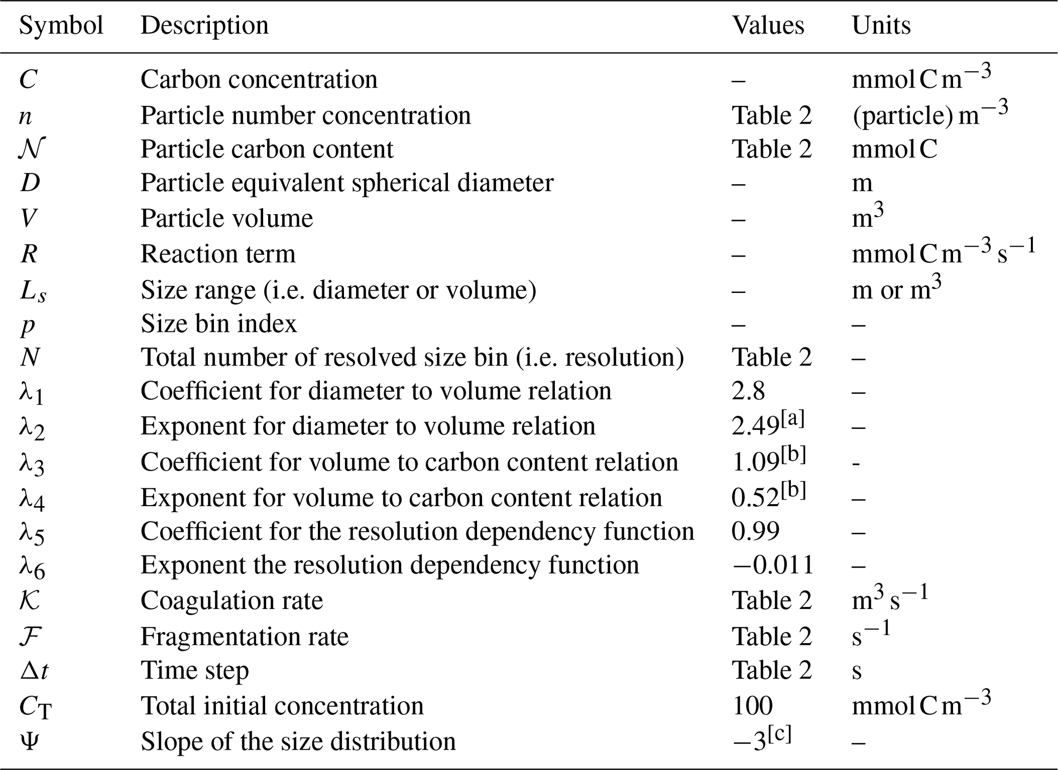
Note that other particle properties (e.g. diameter, volume, density) are similarly interpreted as a bin-averaged value. For example, the particle diameter corresponding to a given bin can be defined by . This diameter can in turn be used to determine the particle volume using an allometric relationship such as (Jackson et al., 1997; Li et al., 1998; Zahnow et al., 2011)1. Using this bin-averaged volume (Vp), the particle content can be redefined as
where λ3 and λ4 are parameters empirically determined through field and laboratory experiments depending on the element chosen (Alldredge, 1998; see Table 1).
The discrete form of Eq. (1) thus becomes
where np is the particle number concentration in p (i.e. the number of particles in p), and N the total number of resolved size bin. In a closed system without sources and sinks of particles, the total concentration, , is required to be conserved over time. The time evolution of the concentration inside a given bin obeys the simple differential form
where Rp represents all reactions occurring in p.
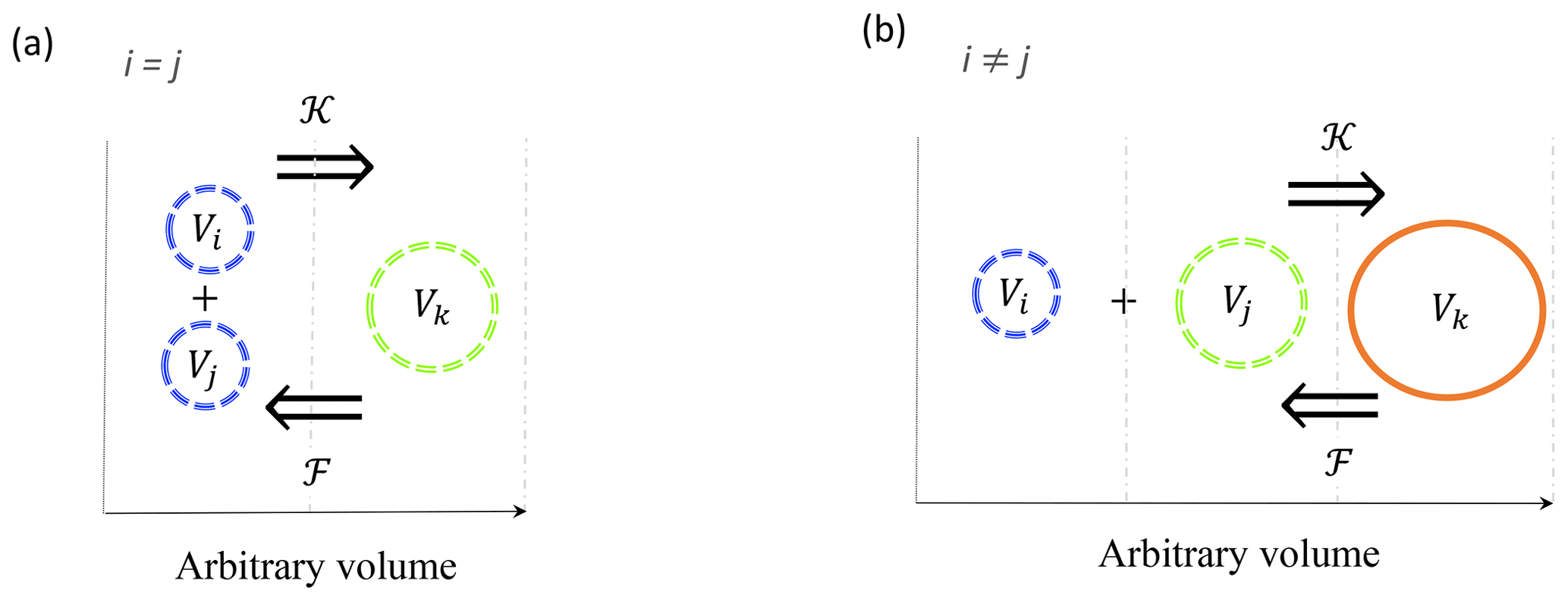
Figure 1Schematic representation of coagulation 𝒦 and fragmentation ℱ reactions between triplets of particles in a linear size discretization. Coagulation is the process by which two particles with indices i and j collide and stick together to form a third, larger one with index k. Fragmentation is the opposite process by which a particle k breaks into two smaller ones i and j. Size bounds are shown by vertical dashed grey lines. Reactions involving two small particles (a) from the same size bin (i=j) and (b) from two different size bins (i≠j) are shown.
2.2 Reaction for a triplet of particles
Coagulation and fragmentation are, by essence, reactions that involve three particles. Coagulation involves two particles, with indices i and j, that collide and stick together to form a third, larger one with index k. Conversely, fragmentation can be considered as the opposite reaction where a particle k breaks into two smaller ones i and j, in line with what was observed by Alldredge et al. (1990) in laboratory experiments. Reactions involving more than three particles can always be decomposed as a sequence of triplet reactions. Note that i and j can originate from identical or different size bins. In a linear size discretization, by definition, the k index always refers to a particle belonging to a different bin than particles i and j. Then, the volume Vk of particle k resulting from the coagulation of particles i and j=1…k obeys
The reaction is arbitrarily built so that the ith particle is always the smallest one. From this assumption, the coagulation reaction can be written as , while fragmentation is (Fig. 1). However, in the case of a nonlinear size discretization, this rule might be violated and this situation is discussed in Sect. 2.6.
In this model, the rules described above for particles will be applied on the bins' discrete spectrum of Eq. (5). For example, in a coagulation reaction implying a given triplet of bins (), the rate of change of the concentration in i will depend on that of j, and they will conjointly prescribe the rate of change of k. Such a reaction for a triplet of bins can be interpreted as multiple reactions for triplets of particles that can be found in their respective bins (). For a reaction implying a given triplet of bins (), the evolution of the concentration in each bin is described by the following set of differential equations:
is a triplet operator that represents both coagulation and fragmentation reactions acting on a given bin:
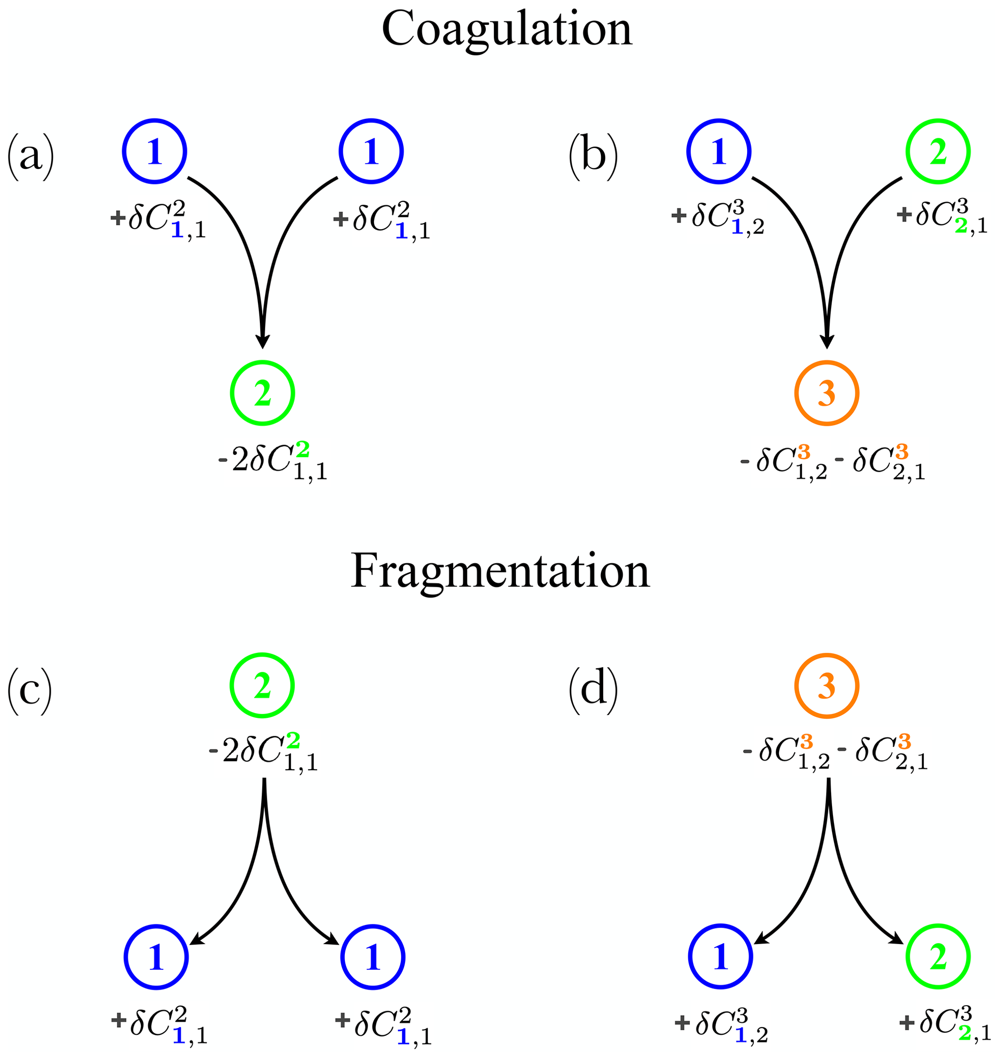
Figure 2Examples of individual reactions for a triplet of bins: (a, b) for coagulation only, assuming ℱ=0 and (c, d) for fragmentation only, assuming 𝒦=0 in Eq. (9). Panels on the left (a, c) involve terms of the diagonal matrix Di=j (Eq. 10), while panels on the right (b, d) involve terms of the off-diagonal matrices B (Eq. 11) and T (Eq. 12) in Sect. 2.3. Different colours (blue, green and black) represent different size bins.
A bold index indicates the bin on which the reaction applies (see also Fig. 2 for a visual explanation of this convention). By construction, of the total number of k particles involved in the reaction in Eq. (8), half of this number is associated with i and the other half with j (Fig. 2), which explains why we multiply all the terms in Eq. (9) by . 𝒦 is the coagulation rate, while ℱ is the fragmentation rate. Coagulation has been studied extensively in previous works both in atmospheric (Pruppacher and Klett, 2010) and oceanographic contexts (Jackson, 2001). It may be decomposed in a combination of a sticking probability and three main collision mechanisms (Kiørboe et al., 1990; Ackleh, 1997; Engel, 2000; Jackson, 2001): Brownian motion, fluid velocity shear and differential settling. Fragmentation (ℱ) can be driven by biology, e.g. related to zooplankton activities such as grazing (Banse, 1990; Green and Dagg, 1997), and swimming behaviour (Dilling and Alldredge, 2000; Stemmann et al., 2000; Goldthwait et al., 2004), or driven by physics, e.g. scales of turbulence (Alldredge et al., 1990; Kobayashi et al., 1999).
Table 1Model variables and parameters.
2.3 Reaction matrices
Let us now consider a set of discrete bins (p) that are linearly incremented and have indices (i,j) running from 1 to N. By construction, this yields reactions for k ranging from k=2 to 2N (i.e. 1+1 to N+N). To account for the concentration evolution associated with all possible reactions, we define four matrices built from the triplet operator () defined earlier, Di=j, Bi,j, Tj,i and Fi,k, referring to diagonal, bottom, top and final matrices, respectively.
Matrix Di=j has dimensions N×N and accounts for reactions in which the two particles have the same size (i=j) (Fig. 2a and c):
The square brackets above indicate the matrix dimensions. Matrix Bi,j accounts instead for all reactions acting on i only (where i<j, Fig. 2b and d):
while Tj,i accounts for those acting on j only (where j>i, Fig. 2b and d):
The fourth matrix contains all the reactions acting on k, which has dimensions N×2N, and is given by
In F, the double line separates the resolved size range (above) from the unresolved one (below). The latter contains reactions involving particle sizes outside the resolved size range of the spectrum (i.e. reactions for which k>N).
The unresolved range
Solution strategies to parameterize reactions in the unresolved range must obey two basic rules: (i) they must conserve the total concentration (CT) in absence of external sources and sinks of particles and (ii) they must limit the unbounded growth of the particle size due to coagulation. Here we propose a simple closure to account for the reactions in this range. In order to comply with conservation of the total concentration in the size range (Ls), at least one new bin must be added in which concentration fluxes in and out of the resolved range are stored. Moreover, in order to avoid unbounded growth of the size range due to coagulation, this extra bin must not be allowed to further coagulate with itself or any of the other particles sizes. As such, all reactions that fall into the unresolved range will be accounted for in a single additional bin for which coagulation is prohibited but fragmentation back into the resolved range is allowed. This extra bin can thus be interpreted as an average of all the reactions in the unresolved range () and will be referred to as . Applying this to Eqs. (10)–(13) yields matrices with dimensions :
where ΔC=2δC when i=j and δC otherwise, and 𝒦=0 in ΔC for . Equation (14) includes all reactions acting on either i or j, while Eq. (15) includes all reactions acting on k. Since the unresolved range only involves reactions acting on k, all the terms below the double line in Eq. (14) are set to zero. Moreover, each term of the last row in Eq. (15) can be viewed as a sum over all the elements of a given column below the double line in Eq. (13). Note that, for simplicity, we choose to add only one extra bin in the unresolved range, but one could alternatively choose to add up to N bins in order to improve this parametrization.
2.4 Summary of all reactions
Based on the matrices (Eqs. 14 and 15) and specific reaction rules previously described, the reaction vector Rp, representing all the reactions for a given bin () is given by
where U is a unit vector with dimension [N],
Coag and Frag in Eq. (16) are used to explicitly show the sign of the coagulation and fragmentation reactions from Eq. (9). In other words, coagulation is removing concentration from p in Xp+Yp, while adding concentration to p in Zp (and conversely for fragmentation). Equation (16) can be rewritten as a sum of the following series:
where ΔC=2δC when p=2i and δC otherwise. An example of a complete set of reactions with N=4 and its additional bin is shown in Fig. 3.
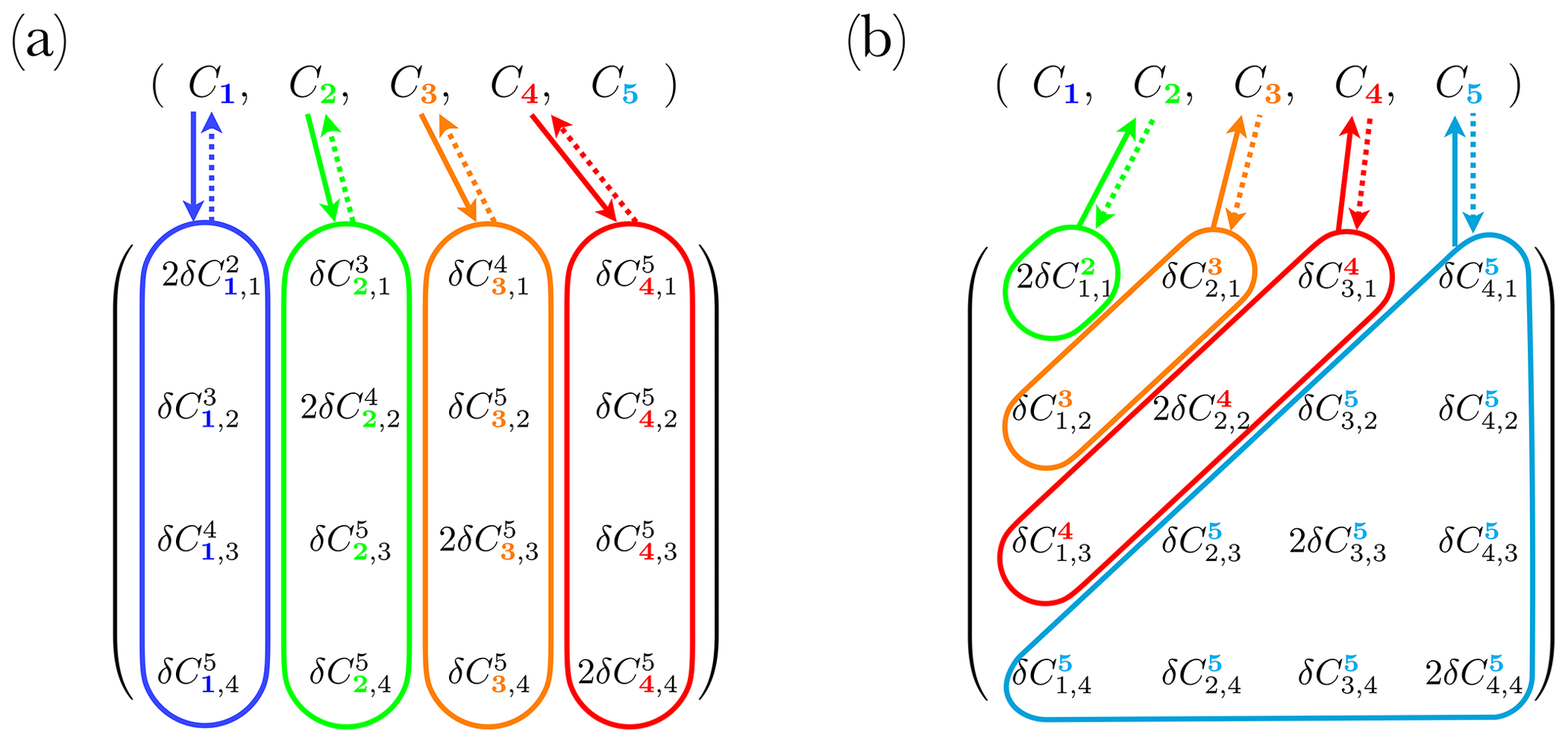
Figure 3Example of a complete set of reactions applied to N=4 size bins, with an additional class . Concentration evolution vectors are shown on top with the four size bins defined by the size range, and the last one representing the size bin . Bottom matrices are modified versions of (a) (Eq. 14) and (b) F (Eq. 15). Coloured areas and arrows indicate an exchange with the concentration vector. Solid and dashed arrows indicate coagulation and fragmentation reactions, respectively.
Focusing on the resolved range only, Eqs. (16) and (18) can be combined to yield a discrete version of the generalized Smoluchowski equation (e.g. von Smoluchowski, 1916; Hansen, 2018):
where δip is the Kronecker delta function that is equal to 1 for i=p and zero otherwise. Notice that the above equation gives the rate of change of concentration, whereas the traditional formulation for the Smoluchowski equation is written in terms of the number of particles. Equation (19) can thus be reformulated in terms of the number of particles as
The factor of in the second term ensures that the combination of two particles yields a single larger particle. This is in contrast to the concentration, for which the combination is additive (see Eq. 8).
2.5 Robustness to resolution
For a discrete representation of the full size range, Ls, larger values of N imply higher resolution of the size spectrum. The total number of reactions of the system described above increases with the size of the reaction matrices, N(N+1), which is nearly a quadratic function of resolution. On the other hand, coagulation and fragmentation are, respectively, quadratic and linear functions of concentration, as shown in Eq. (9). Since concentration is itself a quantity that depends on resolution (Eq. 5), an asymmetric response between coagulation and fragmentation to changes in resolution is expected.
In order to build an intuition on the effect of resolution on the reactions, consider a conservative system with a given total concentration, , and a linear size discretization such that both the particle content and concentration are constants given by 𝒩p=1 and , respectively. To further simplify, assume that the rates of coagulation and fragmentation are constants given by 𝒦 and ℱ, respectively. For a conservative system, the sum of all reactions integrates to zero, i.e. , such that CT remains constant at all time. Since the sum of all reactions does not allow to keep track of the total concentration exchanged along the spectrum, we instead define from Eq. (16) the total reaction amplitude as
and since
where the first term on the right-hand side is the total coagulation amplitude and the second term is the total fragmentation amplitude. In this simple example, dependence to resolution is revealed through the respective prefactors and (N+1). It thus becomes obvious that fragmentation is more sensitive to resolution than coagulation. This result can be explained a posteriori if we notice that the total number of reactions is nearly quadratic with N, while the coagulation concentration is proportional to N−2, cancelling most of the variation with N. In contrast, the fragmentation concentration is proportional to N−1, which yields a larger residual dependence on N. To counterbalance this dependence on resolution, the reaction terms are divided by their respective resolution-dependent coefficients such that
While the general case with non-constant contents and concentrations yields a similar qualitative dependence on N, this simple parametrization produces significant biases in the nonlinear experiment (E2) described in the Sect. 4.2. Thus, a more exhaustive study on robustness to resolution is needed in order to improve this parametrization, and solutions strategies are discussed in Sect. 4.3.
2.6 Nonlinear size spectrum
For simplicity, we chose to describe the above framework using a linear size discretization (i.e. where bins are equally distributed along the size range). However, this choice was arbitrary and we now generalize the framework to a nonlinear size discretization, which is a more natural choice for representing marine particles. A nonlinear size discretization can be seen as local variations of the resolution in the full size range. For example, for a given total number of bins, N, switching from a linear to a logarithmic spacing increases resolution for the small particles, while decreasing it for the large particles. Intuitively, this choice seems better suited to represent marine particles that have a wider variety of microscopic than macroscopic particles.
In this context, the main difference with the framework described in the previous sections is that volume conservation can be violated when using a nonlinear size spectrum; i.e. Eq. (7) is no longer valid. Although counterintuitive, this does not imply however that mass conservation is necessarily violated. Consider, for example, a simple nonlinear discretization where bins are each separated by an order of magnitude (1, 10, 100 µm3, etc.). Coagulation of particles belonging to bins 1 and 10 µm3 would ideally produce a particle size of 11 µm3. However, since 11 µm3 is much closer to bin 10 µm3 than bin 100 µm3 (the next larger bin), all the concentration associated with this reaction will fall into the 10 µm3 bin, thus violating volume conservation, yet conserving the concentration associated with the reaction. We thus modify Eq. (7) to allow that the resulting size of a coagulation reaction is not required to be strictly equal to the sum of the two reacting particles (and conversely for fragmentation), i.e.
The main consequence of Eq. (23) is that it modifies the reaction matrices (Eqs. 14 and 15). In Eq. (14), only the k indices will be modified by a nonlinear discretization. In Eq. (15), the elements themselves will be redistributed on different rows of the matrix. For a logarithmic discretization that enhances resolution towards smaller particles, elements will be moved upwards in the F matrix as an increased number of reactions yield . For example, could be switched from the third row using a linear spectrum to in the second row using a logarithmic spectrum. Conversely, elements will be moved downwards in the F matrix if a discretization that enhances resolution towards larger particles is chosen. Here, we do not explicitly write the matrix encompassing all possible cases since this would be unnecessarily complex. The construction of the reaction matrices (Eqs. 14 and 15) is done numerically at the beginning of our algorithm (see Gremion and Nadeau, 2021).
2.7 Application to a plankton ecosystem model
The framework presented here gives rise to N variables that together represent detritic particulate matter. Like other variables of plankton ecosystem models, these additional variables must be treated as Eulerian tracers submitted to diffusive and advective transport. In a typical three-dimensional OGCM, the evolution of the carbon concentration Cp (mmol C m−3) belonging to the size bin p is given by
where is the velocity field and . The terms on the right side are (i) the advective flux convergence, (ii) the diffusive flux divergence, with K the turbulent diffusivity, (iii) the background vertical advection due to the settling velocity wp associated to size bin p, (iv) the sources and (v) the losses of detritic matter associated with other biogeochemical processes, and (vi) the reaction term, Rp, representing coagulation and fragmentation derived in this paper (Eq. 16). The three-dimensional velocity u is provided by equations driving geophysical fluid dynamics. The vertical settling velocity, wp, is here assumed constant for a given size but can vary considerably from one size to another as it strongly depends on particle properties such as its volume, density and porosity. Therefore, Cp does not vary due to differential settling (divergence or convergence), but CT can through the action of the reaction term, Rp. In order to focus uniquely on the reaction term, Rp, we do not solve Eq. (24) explicitly in this work and leave this for a subsequent study. In the following, we use the simplified zero-dimensional form to investigate the robustness of the proposed framework on the resolution, N.
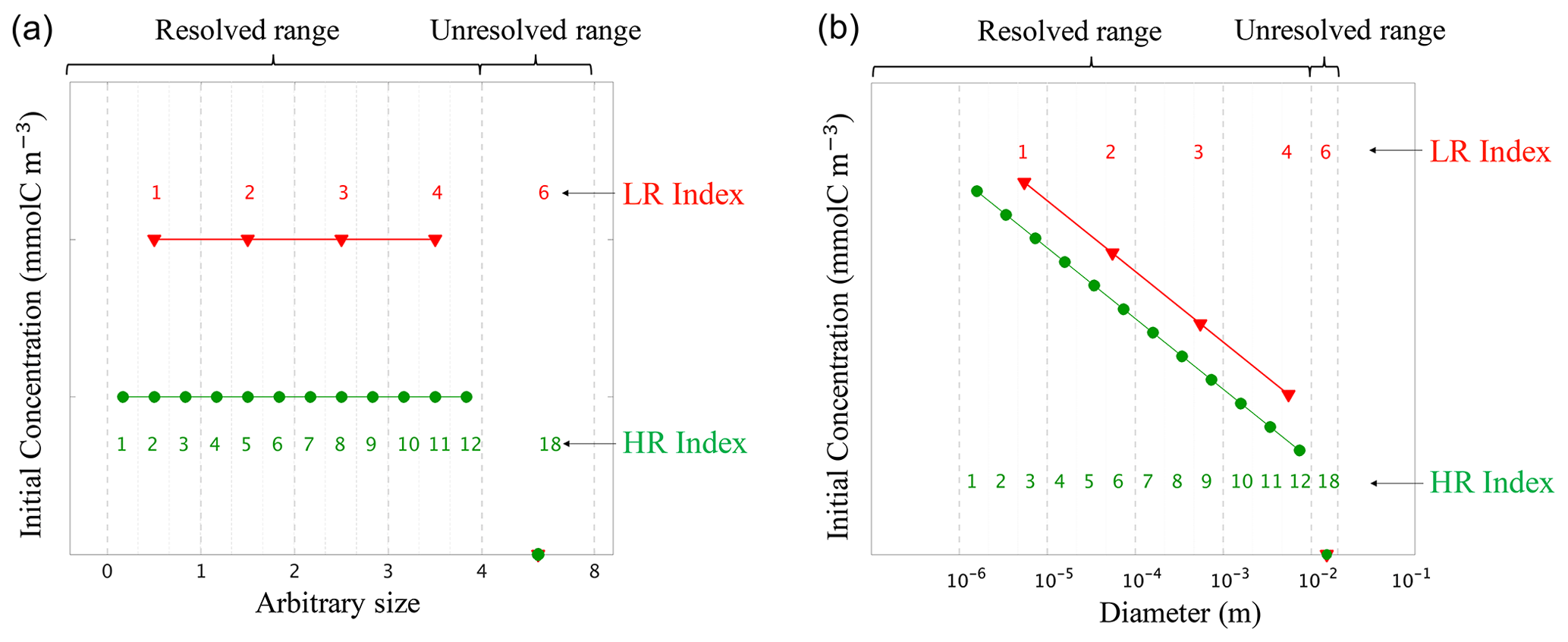
Figure 4Initial conditions for (a) the linear size discretization (E1) and (b) the nonlinear size discretization (E2), for the two resolutions. The low resolution (LR), in red, has N=4 size bins plus one unresolved size bin , while the high resolution (HR), in green, has N=12 size bins plus one unresolved bin . This is an illustrative example as the HR simulations performed in this paper with N=400. Size bin bounds are shown by vertical dashed grey lines. All simulations are initialized with the same total carbon concentration CT (see Table. 1). The initial concentration is spread uniformly over the resolved range for E1-LR and E1-HR, and following a power law for E2-LR and E2-HR (see Table. 2). No concentration is initialized in the unresolved size bin. As HR has more size bins than LR, concentrations values are consequently lower as determined by in E1. Concentrations are prescribed to the middle size value of a given bin.
Two model configurations are set up to study detritic carbon concentration (C) dynamics experiencing coagulation and fragmentation reactions using the previously described model. The first configuration, named E1, uses a linear size discretization over the arbitrarily chosen range of 0 to 8 (Fig. 4a). The second configuration, identified as E2, uses a nonlinear size discretization that more realistically represents particle number distributions observed in the ocean, i.e. particle size from D1 = 1 µm to DN = 1 cm (Stemmann et al., 2004; Monroy et al., 2017) (Fig. 4b). Each set of experiments within the configurations is performed using two different numbers of size bins (N) in order to study the impact of resolution on the model. The high-resolution (HR) simulation uses N=400 size bins, while the low-resolution (LR) simulation uses N=4. An additional bin having an index value of is added to represent the unresolved size range, which increases the total number of bins to N=401 and N=5, respectively. For each resolution, three simulations are performed: two simulations where coagulation (K) and fragmentation (F) are considered separately, and one simulation where they are combined (KF). In total, 12 simulations are performed with parameter values summarized in Tables 1 and 2.
Table 2Numerical experiments and associated model configurations and parameters.

3.1 Initialization
For each configurations, all experiments are initialized from a reference distribution at very high resolution (i.e. bins) that is meant to represent an ideal distribution. This discretization is indicated by the symbol †. The total carbon concentration is set to CT = 100 mmol C m−3, and initial concentrations, Cp(t=0), are then initialized for HR and LR by integrating on the reference distribution using a discrete version of Eq. (3):
where p refers to indices of the HR and LR discretizations and q to indices of the reference distribution. For HR and LR in configuration E1, the initial carbon concentration of the reference is uniform (i.e. ) as for the particle carbon content (𝒩p=1). The chosen time step is Δt = 86 400 s, and it is run for one time step.
In E2, the reference is initialized with a power-law-distributed carbon concentration of the form (McCave, 1984; Li et al., 2004)
where n is the number of particles of diameter D and Ψ is the slope of the distribution, by connecting with Eq. (5). Unlike in E1, particle carbon content is set to a size-dependent function following Eq. (4). HR and LR initial carbon concentration distributions are then obtained following Eq. (25), and the model is integrated for a day with a time step Δt = 3600 s.
In both configurations (E1 and E2), in order to compare results from both simulations and assess the resolution dependence of the model, HR carbon concentrations are mapped to the LR discretization following Eq. (25). Moreover, in order to simplify the problem and to focus only on the resolution dependence of the framework, coagulation and fragmentation rates, 𝒦 and ℱ, respectively, are set to constant values (Table 2).
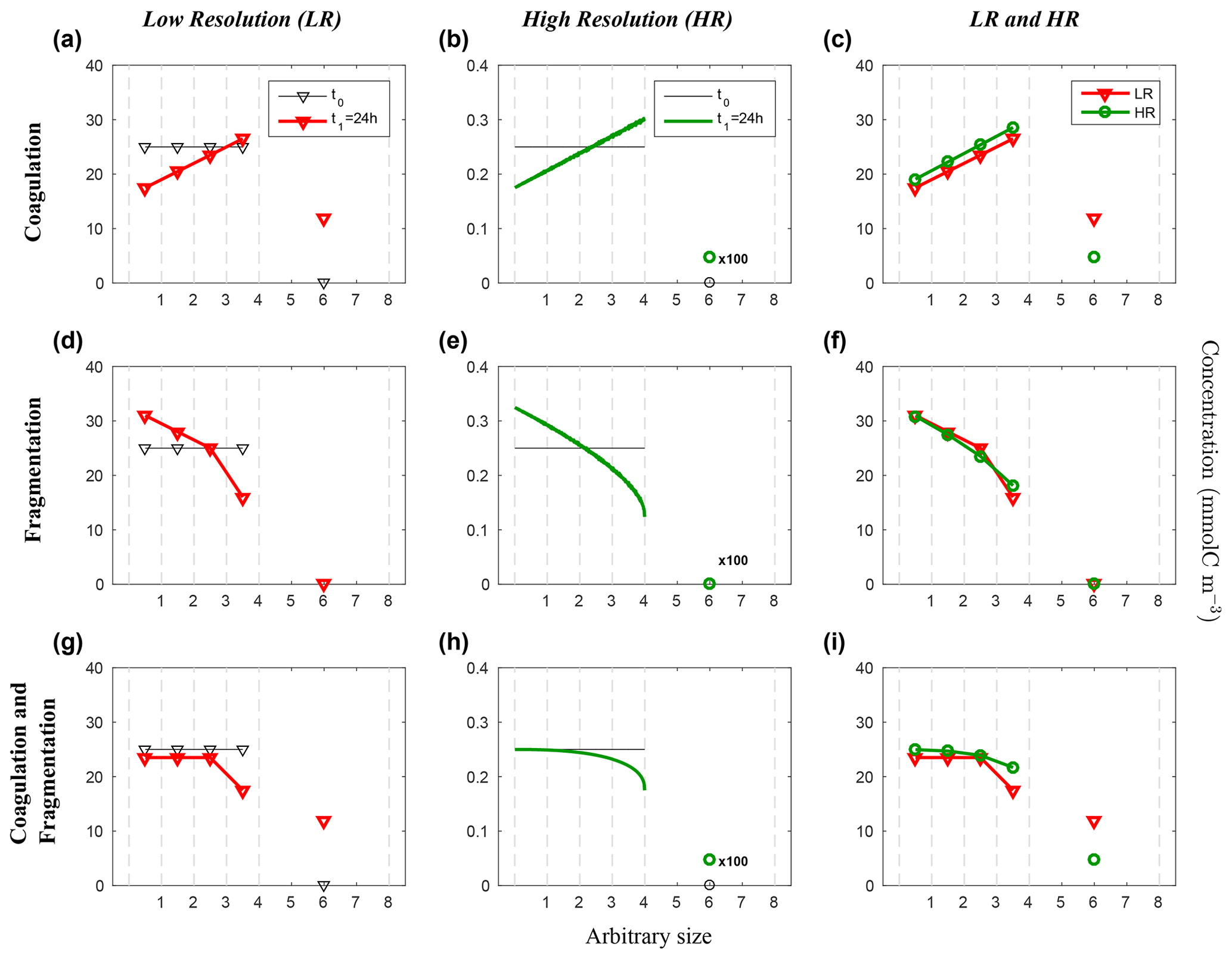
Figure 5Evolution of the carbon concentration distribution over the size range in the linear size discretization configuration (E1) as function of the arbitrary size. Our three sets of reaction simulations are represented: coagulation only (a–c), fragmentation only (d–f) and when both reactions are combined (g–i). The left column (a, d, g) represents our LR setup, the middle column (b, e, h) the HR one and the right column (c, f, i) the comparison of the HR carried back to LR (see Eq. 25 in Sect. 3.1 for details). Y abscissas are different between our resolutions and are set to allow an easy comparison. For each panel, the initial time step t0 is in black and the final time step t1 = 24 h appears in red for LR and in green for HR. As it is the linear size discretization configuration, the LR resolved bins indexes equal the arbitrary size. Solitary points represent the size bin for both resolutions, as they represent the average of a larger number of size bins (LR: 5 to 8, and HR: 401 to 800) than the ones in the resolved range. Notice that the final carbon concentration in the unresolved bin of the HR experiment is divided by a factor of 100 in order to fit in the y scale. As detailed in the methods (Sect. 2.3.1), both coagulation and fragmentation reactions occur in the resolved range but only fragmentation occurs in the unresolved range. For further details, refer to the legend of Fig. 4.
4.1 Linear discretization
Figure 5 shows the results from the linear size discretization (E1), for both LR and HR simulations and for coagulation and fragmentation considered separately as well as simultaneously.
Starting with initial uniform carbon concentration distribution, coagulation leads to a reduction of Cp in small size bins and an increase in larger ones for both LR and HR, resulting in a linearly increasing distribution of Cp over the resolved size range (p=1 to N, Fig. 5a, b). The largest accumulation of Cp appears in the unresolved size range () for both LR and HR simulations. Notice that the carbon concentration in the unresolved bin of the HR experiment is divided by a factor of 100 in order to fit in the y scale. However, a smaller amount of particles end up in this range in the HR simulation compared to the LR (Fig. 5c), which is associated with larger final concentrations Cp in the resolved range for HR since the model is conservative by design. The final carbon concentration distributions are nonetheless very similar considering the very large difference in the number of bins between LR and HR.
In contrast with coagulation, fragmentation yields a reduction of Cp in larger size bins to the benefit of an increase in the small ones (Fig. 5d–f). Only very small differences of Cp are noticeable between LR and HR over the resolved range (Fig. 5f), suggesting that fragmentation is very weakly dependent on the size range resolution when a linear discretization is used. As the unresolved range is initialized to zero, and fragmentation does not allow particle to increase in size, remains zero for both simulations.
When both reactions are combined and act simultaneously, they nearly compensate each other in small size bins in both simulations (Fig. 5g and h) but to a greater extent in the HR case. For larger size bins however, fragmentation seems to operate nonlinearly and more strongly than coagulation, leading to a smaller carbon concentrations related to large particles compared to the initial value. The comparison (Fig. 5i) shows a significantly greater Cp in each resolved size bins for HR compared to LR, but it is the inverse for the unresolved range. This is explained by the asymmetry that exists in the mathematical formulation of coagulation and fragmentation (Eq. 9), with the former being a quadratic function of concentration, while the latter is a linear function. Overall, despite the fact that coagulation and fragmentation do not compensate for each other, which is not a prerequisite in the model, the dependence on the number bins for a given range of particle sizes is quite weak when using a linear discretization.
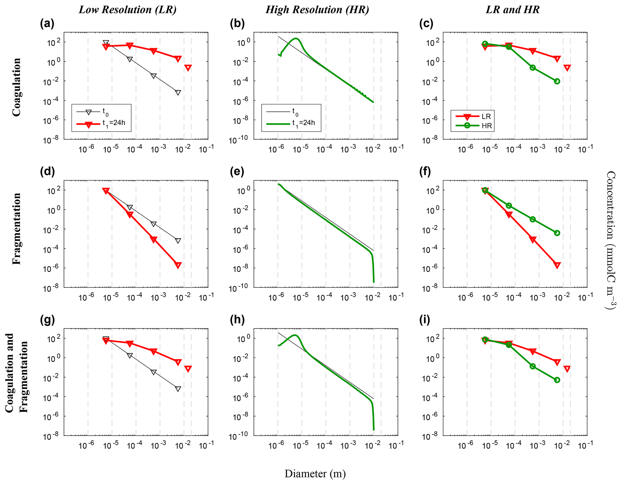
Figure 6Evolution of the carbon concentration distribution over the size range in our nonlinear size discretization configuration (E2) as function of diameters. Our three sets of reaction simulations are represented: coagulation only (a–c), fragmentation only (d–f) and when both reactions are combined (g–i). The left column (a, d, g) represents our LR setup, the middle column (b, e, h) the HR one and the right column (c, f, i) the comparison of the HR carried back to LR (see Eq. 25 in Sect. 3.1 for details). Y abscissas are different between our resolutions and are set to allow an easy comparison. For each panel, the initial time step t0 is in black and the final time step t1 = 24 h appears in red for LR and in green for HR. Solitary points represent the size bin for both resolutions, as they represent the average of a larger number of size bins (LR: 5 to 8, and HR: 401 to 800) than the ones in the resolved range. Notice that the final carbon concentration in the unresolved bin of the HR experiment is divided by a factor of 100 in order to fit in the y scale. As detailed in the methods (Sect. 2.3.1), both coagulation and fragmentation reactions occur in the resolved range but only fragmentation occurs in the unresolved range. For further details, refer to the legend of Fig. 4.
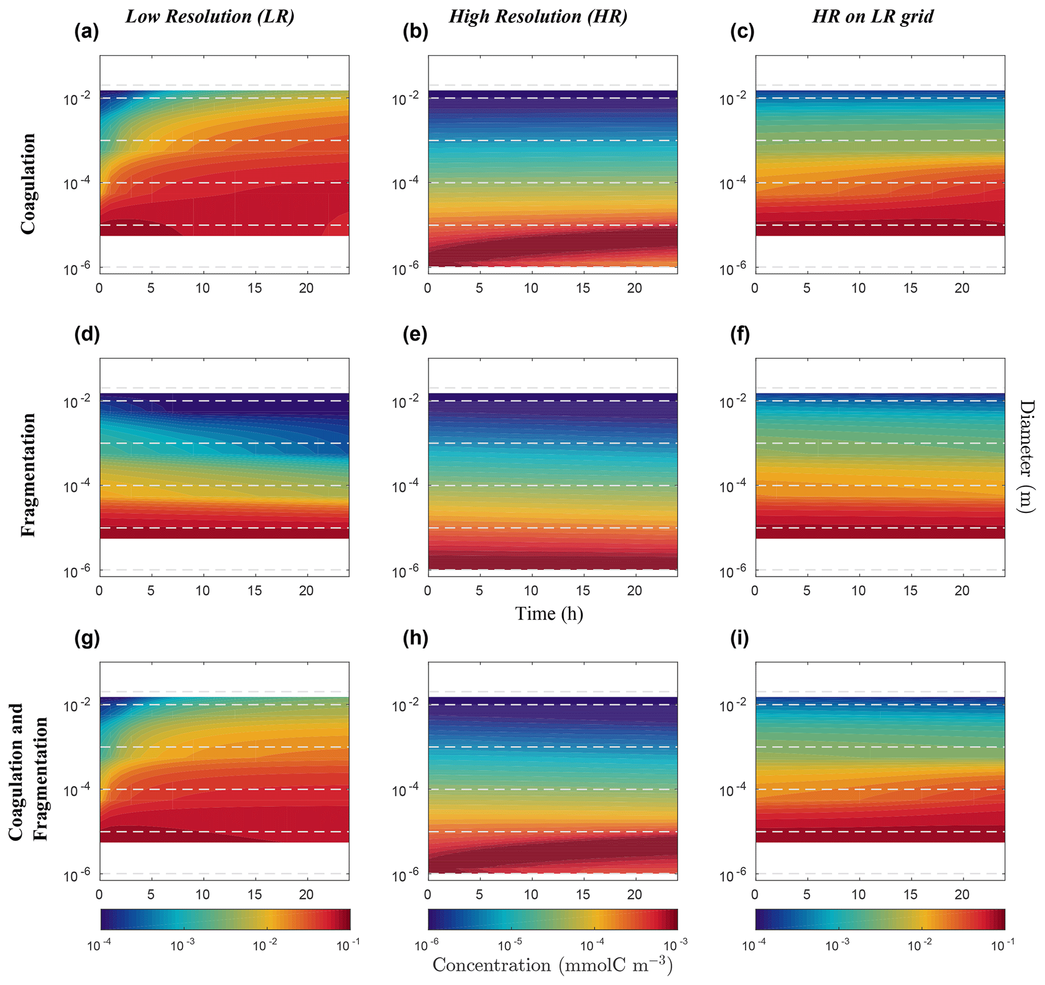
Figure 7Hovmöller plots of carbon concentration as a function of particle diameter over a 24 h period for the nonlinearly discretized configuration (E2). Simulations for coagulation and fragmentation considered separately (on top and middle lines, respectively) and combined (on bottom line), and for LR (left column) and HR (middle column), are shown. The right column shows the HR when mapped to the LR grid. Note the logarithmic scale for the vertical axis representing particle diameter (m) and for the colour scale representing carbon concentrations (mmol C m−3). Concentration value scales are different between our resolutions and are set to allow an easy comparison. Dashed lines represent the bounds of each LR size bin. Dealing with size spectrum logarithmic scale, middle size bin concentration value will induce no concentration data in the lower bound of the first size bin in the LR (a, d, g) and for the HR mapped to the LR grid (c, f, i).
These results demonstrate that in a linearly size discretized configuration, the model is reasonably independent of the resolution when coagulation and fragmentation are used independently or combined (Fig. 5). They show however the importance of considering the unresolved size range in the model design, which guarantees mass conservation and unbounded growth due to coagulation.
4.2 Nonlinear discretization
We now consider the results from the nonlinear size discretization model (E2), shown in Figs. 6 and 7. Recall that instead of a uniform Cp distribution, the model is initialized with a distribution that is exponentially decreasing over a size range from 10−6 m to 10−2 m, thus spanning 4 orders of magnitude (Eq. 26, Table 2). In this case, results differ as a function of resolution for the reactions taken separately or combined. All LR simulations (K, F and KF) react more strongly than the HR ones.
Focusing first on the resolved range in the coagulation-only experiment, we observe a diminution of Cp in the smaller size bins and an accumulation in the larger size bins in LR simulation (Fig. 6a). However in HR, this distribution pattern is limited to a small range of sizes between 10−6 m and 10−4 m (Fig. 6b). In addition, no significant accumulation of concentration is observed in the largest size bins, and by extension neither into the unresolved range (). This leads to a difference of Cp regarding the larger size bins between LR and HR when mapped on the same grid (Fig. 6c), with the LR overestimating carbon concentration for larger size bins. Figure 7 shows the time evolution of the distributions of Fig. 6. In the LR case, the initial response (roughly 2 h) is characterized by a fast timescale, followed by a slower response during the rest of the simulation (Fig. 7a). In contrast, in the HR case, the response is localized in the small size range and only the slower response is observed (Fig. 7b). While attenuated, these biases are still clearly visible when HR is remapped on LR (Fig. 7c).
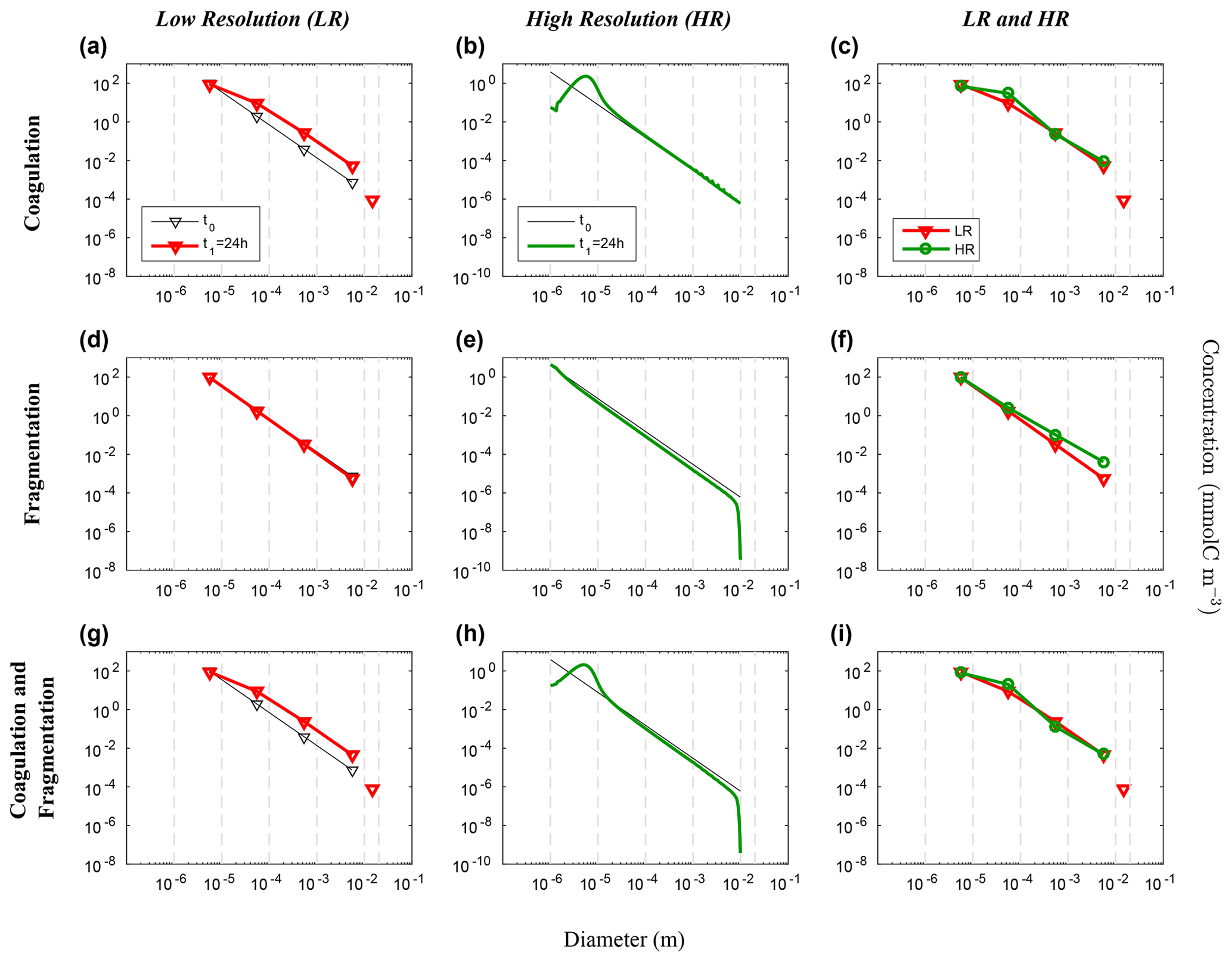
Figure 8Evolution of the carbon concentration distribution over the size range in our nonlinear size discretization configuration (E2) as function of diameters when the function reducing resolution dependency is implemented (Eq. 27). Our three sets of reaction simulations are represented: coagulation only (a–c), fragmentation only (d–f) and when both reactions are combined (g–i). The left column (a, d, g) represents our LR setup, the middle column (b, e, h) the HR one and the right column (c, f, i) the comparison of the HR carried back to LR (see Eq. 25 in Sect. 3.1 for details). For each panel, the initial time step t0 is in black and the final time step t1 = 24 h appears in red for LR and in green for HR. For further details, refer to the legend of Fig. 6.
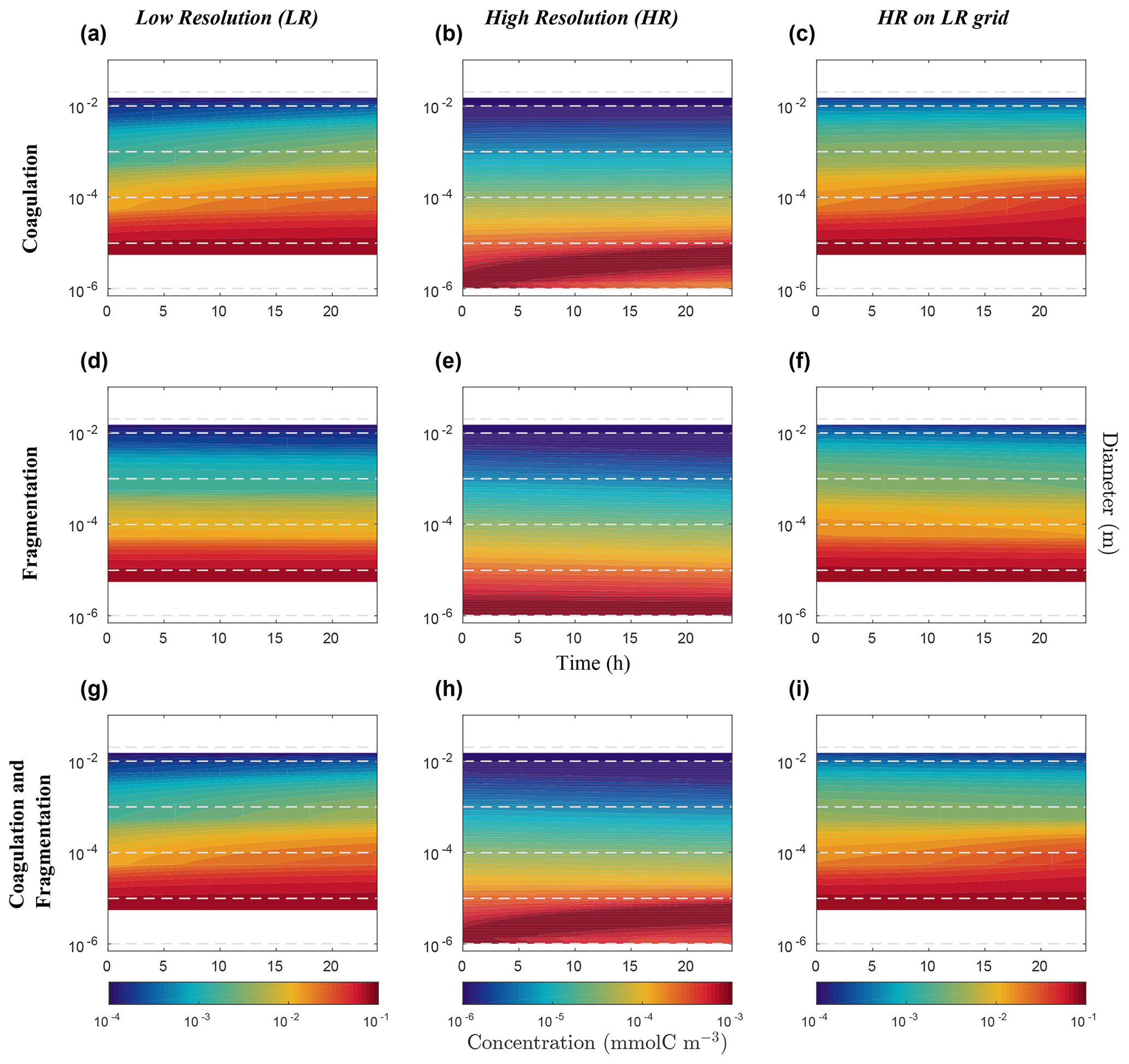
Figure 9Hovmöller plots of carbon concentration as a function of particle diameter over a 24 h period for the nonlinearly discretized configuration (E2) with the application of the function which attempt to reduce the dependency to the resolution of our model (Eq. 27). Simulations for coagulation and fragmentation considered separately (on top and middle lines, respectively) and combined (on bottom line), and for LR (left column) and HR (middle column), are shown. For further details, refer to the legend of Fig. 7.
Results for fragmentation only yield a similar biases between the LR and HR cases. Reactions are magnified in LR compared to HR (panels d–f of Figs. 6 and 7). When both reactions are combined, coagulation dominates over fragmentation to explain most of the observed changes in distribution of the LR simulation (Fig. 6g). In HR, both coagulation and fragmentation have localized effects on the smallest and largest size ranges (Fig. 6h). The comparison of HR vs. LR shows a pattern that is similar to the comparison between resolutions for the coagulation reaction (Figs. 6i and 7i). This indicates that coagulation dominates over fragmentation, which is expected for an initial concentration distribution that is highly skewed towards small particles.
These simulations demonstrate that when using a nonlinear size discretization and a nonlinear initial carbon concentration distribution, the model behaviour is significantly dependent on resolution. To attenuate this dependence, which arises from the asymmetry between coagulation and fragmentation, we propose adding and tuning a penalty function that will compensate this difference as N varies.
4.3 Resolution dependency function
The residual dependence of the model to resolution in the nonlinear discretization arises mainly from the fact that the prefactors used in Eq. (22) are derived from a linear analysis, which yields an asymmetry between coagulation and fragmentation. To minimize the effect of this asymmetry, we propose multiplying both reaction terms by a resolution-dependent function f(N) that is positive and monotonically varies between a value to be determined at low N and 1 for N→∞. For simplicity, we here assume an exponential function of the form
with λ5 and λ6 positive constant parameters that were determined empirically (see Table 1).
Simulation results obtained with this correction factor (Figs. 8 and 9) show that both LR and HR simulations now agree much better. The LR simulation is the one that is the most impacted by this change (Fig. 8a–c), as and . Comparing Fig. 6c, f and i with Fig. 8c, f and i, it is clear that a carefully chosen penalty function such as that in Eq. (27) can significantly reduce the error attributed to a number of size bins as low as four. The fundamental cause of the resolution dependency seems to be linked with the nonlinear size discretization, but it is not clear how the penalty function can be determined in a simple way from prior knowledge. Is this solely dependent on the choice of discretization, or is it also dependent on how particles are distributed along that spectrum? This remains an open question.
We have developed a new 0-D numerical model for representing coagulation and fragmentation as an interaction between three particles of arbitrary sizes. Particles are categorized in size bins that can be linearly or nonlinearly distributed along a given size spectrum. In the linear configuration, E1, the total volume of suspended particulate matter (i.e. the sum of the volume of all individual particles) is also conserved. However, this is not strictly the case in the nonlinear configuration, E2, because it can happen that two particles of two different size bins can end up in the same size bin as the biggest one. By construction, the total concentration of carbon carried by particles is conserved over the resolved and unresolved range. The unique arbitrary size bin offers (i) boundaries to avoid any exponential growth of the size range and (ii) reduces falsified carbon concentration estimation in the larger size bins. When absent, accumulation of particles was observed (exploratory studies of our current work which are not shown). This caveat is present in models using the sectional approach, the solution of which is to increase the number of bins, as described by Burd (2013).
Coagulation has a quadratic dependence on particle number concentration participating to the reaction, while fragmentation has a linear dependence on the particle number concentration. The linear configuration has a very weak dependence on the size spectral resolution (number of size bins N for a given size range). The nonlinear configuration has a significant dependence to resolution. This dependence can be overcome by multiplying both reaction terms with a function f(N) such that f(N)→1 when N→∞. However, further work is required to unearth what is causing the dependence, as the assumption made that reactions need to be divided by the inverse dependent resolution coefficient (Eq. 22) for both linear and nonlinear cases was partly wrong. The surmise that Cp will be equally distributed between the size bins (i.e. ) is not respected in the nonlinear case as distribution assigned is nonlinear over the size bins (Eq. (26), i.e. ) in addition to be coupled to a nonlinear size discretization. The presented attempt to rectify this wrong assumption via the elaboration of the function (Eq. 27) for the nonlinear case allows prospects to thrive and reassure that solutions exist. Despite this, the model succeeds in representing the evolution of the size of suspended particulate matter due to the simultaneous action of coagulation and fragmentation using a low number of size bins (N=4). This is comparable to biogeochemical models of low (e.g. Fasham et al., 1990, with seven state variables, or Neumann, 2000, with nine) to moderate complexity (e.g. Aumont et al., 2015, with 24 prognostic variables, or Ward et al., 2012, with more than 50). However, the sensitivity of our model outcomes to many arbitrary constant parameters needs to be profoundly investigated, as some of them may be size dependent and therefore vary along the size range. Such parameters are the coagulation rate and associated stickiness of particles (𝒦, Eq. 9) and the fragmentation rate (ℱ, Eq. 9). Other parameter values, such as the slope of the particle distribution (Ψ, Eq. 26) and parameters relying on the carbon content estimation of each particles (𝒩, Eq. 4), were chosen according to literature, determined through field or laboratory studies for specific geographic regions or ecosystem states. The total initial carbon concentration over the size range (CT) will also require deeper investigation, as by acting jointly with other parameters it may affect reaction thresholds in the model, and the final outcomes and conclusions. Lastly, the role of coagulation and fragmentation reactions on the cell density behaviour along the size range will be required (Gregory, 1997) in the parameterization of the settling velocity for each detritic state variable implemented. This step will be required to incorporate the model in a 1-D environment coupled to physical fields. Ultimately, when reliably parameterized, this model will be coupled to an upper-trophic-level ecological model and OGCMs that will enable addressing further questions related to the fate of particle evolution with depth.
Through our approach, a balance between a low computational cost and a proximity to particulate organic matter ecological dynamics expected to be found in the ocean was fulfilled. This is a first attempt to fill the knowledge gap underlined by Boyd et al. (2019) by offering a model of particle transformations to incorporate in OGCMs. This work, as well as the steps to come, will then offer new perspectives to estimate the downward carbon export in global models, as coagulation and fragmentation reactions will be characterized alongside of other known processes affecting the vertical flux of organic matter (e.g. grazing, remineralization). Thus, comparisons with previous studies will be possible to conclude on the influence to consider or not these often-ignored reactions on the estimation of the biological pump's response to climate change.
The current version of the model and user manual are freely available and can be downloaded from the referenced project page: https://doi.org/10.5281/zenodo.4432896 (see Gremion and Nadeau, 2021). The code concedes to the GNU General Public License v2.0 and is written in Fortran 90 and requires the gfortran compiler. MATLAB 2015b minimum is required to reproduce the figures using the scripts provided in the Zenodo archive.
The data, analysis and figures presented in this paper can be generated using the model files available in the “Code availability” section and user-defined parameters.
GG and LPN co-built the numerical framework and prepared the figures; GG ran the analysis and wrote the text; GG, LPN, CD and DD participated in discussions prior to model setup; LPN, CD, IRS, PA and DD provided edits and reviews during manuscript preparation. DD secured funding to support the development of the model.
The authors declare that they have no conflict of interest.
Publisher's note: Copernicus Publications remains neutral with regard to jurisdictional claims in published maps and institutional affiliations.
The work was conducted within the framework of ArcticNet, a Network of Centres of Excellence of Canada, and of the Quebec Ocean strategic network.
This research has been supported by the Natural Sciences and Engineering Research Council of Canada (NSERC) Discovery Grant to Dany Dumont (grant no. 402257-2013) and Arc3Bio (Marine Biodiversity, Biological Productivity and Biogeochemistry in the Changing Canadian Arctic), an ArcticNet project.
This paper was edited by Sylwester Arabas and reviewed by two anonymous referees.
Ackleh, A. S.: Parameter estimation in a structured algal coagulation-fragmentation model, Nonlinear Anal.-Theor., 28, 837–854, https://doi.org/10.1016/0362-546X(95)00195-2, 1997. a
Alldredge, A.: The carbon, nitrogen and mass content of marine snow as a function of aggregate size, Deep-Sea Res. Pt. I, 45, 529–541, https://doi.org/10.1016/S0967-0637(97)00048-4, 1998. a, b
Alldredge, A. L., Granata, T. C., Gotschalk, C. C., and Dickey, T. D.: The physical strength of marine snow and its implications for particle disaggregation in the ocean, Limnol. Oceanogr., 35, 1415–1428, https://doi.org/10.4319/lo.1990.35.7.1415, 1990. a, b, c
Anderson, T. and Gentleman, W.: The legacy of Gordon Arthur Riley (1911–1985) and the development of mathematical models in biological oceanography, J. Mar. Res., 70, 1–30, https://doi.org/10.1357/002224012800502390, 2012. a
Anderson, T. R.: Plankton functional type modelling: running before we can walk?, J. Plankton Res., 27, 1073–1081, https://doi.org/10.1093/plankt/fbi076, 2005. a
Anderson, T. R., Gentleman, W., and Sinha, B.: Influence of grazing formulations on the emergent properties of a complex ecosystem model in a global ocean general circulation model, Prog. Oceanogr., 87, 201–213, https://doi.org/10.1016/j.pocean.2010.06.003, 2010. a
Aumont, O., Maier-Reimer, E., Blain, S., and Monfray, P.: An ecosystem model of the global ocean including Fe, Si, P colimitations, Global Biogeochem. Cy., 17, 1060, https://doi.org/10.1029/2001GB001745, 2003. a, b
Aumont, O., Ethé, C., Tagliabue, A., Bopp, L., and Gehlen, M.: PISCES-v2: an ocean biogeochemical model for carbon and ecosystem studies, Geosci. Model Dev., 8, 2465–2513, https://doi.org/10.5194/gmd-8-2465-2015, 2015. a
Banse, K.: New views on the degradation and disposition of organic particles as collected by sediment traps in the open sea, Deep-Sea Res., 37, 1177–1195, https://doi.org/10.1016/0198-0149(90)90058-4, 1990. a
Blackford, J. and Radford, P.: A structure and methodology for marine ecosystem modelling, Neth. J. Sea Res., 33, 247–260, https://doi.org/10.1016/0077-7579(95)90048-9, 1995. a
Boyd, P., Claustre, H., Levy, M., Siegel, D., and Weber, T.: Multi-facted particle pumps drive carbon sequestration in the ocean, Nature, 568, 327–335, https://doi.org/10.1038/s41586-019-1098-2, 2019. a
Burd, A. B.: Modeling particle aggregation using size class and size spectrum approaches, J. Geophys. Res., 118, 3431–3443, https://doi.org/10.1002/jgrc.20255, 2013. a
Burd, A. B., Chanton, J. P., Daly, K. L., Gilbert, S., Passow, U., and Quigg, A.: The science behind marine-oil snow and MOSSFA: past, present, and future, Prog. Oceanogr., 187, https://doi.org/10.1016/j.pocean.2020.102398, 2020. a
Butenschön, M., Clark, J., Aldridge, J. N., Allen, J. I., Artioli, Y., Blackford, J., Bruggeman, J., Cazenave, P., Ciavatta, S., Kay, S., Lessin, G., van Leeuwen, S., van der Molen, J., de Mora, L., Polimene, L., Sailley, S., Stephens, N., and Torres, R.: ERSEM 15.06: a generic model for marine biogeochemistry and the ecosystem dynamics of the lower trophic levels, Geosci. Model Dev., 9, 1293–1339, https://doi.org/10.5194/gmd-9-1293-2016, 2016. a
De La Rocha, C. L. and Passow, U.: Factors influencing the sinking of POC and the efficiency of the biological carbon pump, Deep-Sea Res. Pt. II, 54, 639–658, https://doi.org/10.1016/j.dsr2.2007.01.004, 2007. a, b
Denman, K.: Modelling planktonic ecosystems: parameterizing complexity, Prog. Oceanogr., 57, 429–452, https://doi.org/10.1016/S0079-6611(03)00109-5, 2003. a
Denman, K., Brasseur, G., Chidthaisong, A., Ciais, P., Cox, P., Dickinson, R., Hauglustaine, D., Heinze, C., Holland, E., Jacob, D., Lohmann, U., Ramachandran, S., da Silva Dias, P., Wofsy, S., and Zhang, X.: 2007: Couplings Between Changes in the Climate System and Biogeochemistry, in: Climate Change 2007: The Physical Science Basis. Contribution of Working Group I to the Fourth Assessment Report of the Intergovernmental Panel on Climate Change, edited by: Solomon, S., Qin, D., Manning, M., Chen, Z., Marquis, M., Averyt, K., Tignor, M., and Miller, H., Cambridge University Press, Cambridge, UK and New York, NY, USA, availabale at: https://www.ipcc.ch/site/assets/uploads/2018/02/ar4-wg1-chapter7-1.pdf (last access: 28 June 2021), 2007. a
Dilling, L. and Alldredge, A. L.: Fragmentation of marine snow by swimming macrozooplankton: A new process impacting carbon cycling in the sea, Deep-Sea Res. Pt. I, 47, 1227–1245, https://doi.org/10.1016/S0967-0637(99)00105-3, 2000. a, b
Dissanayake, A. L., Burd, A. B., Daly, K. L., Francis, S., and Passow, U.: Numerical modeling of the interactions of oil, marine snow, and riverine sediments in the ocean, J. Geophys. Res.-Oceans, 123, 5388–5405, https://doi.org/10.1029/2018JC013790, 2018. a
Doney, S., Kleypas, J., Sarmiento, J., and Falkowski, P.: The US JGOFS Synthesis and Modeling Project – An introduction, Deep-Sea Res. Pt. II, 49, 1–20, https://doi.org/10.1016/S0967-0645(01)00092-3, 2002. a
Doney, S. C., Glover, D. M., and Najjar, R. G.: A new coupled, one-dimensional biological-physical model for the upper ocean: Applications to the JGOFS Bermuda Atlantic Time-series Study (BATS) site, Deep-Sea Res. Pt. II, 43, 591–624, https://doi.org/10.1016/0967-0645(95)00104-2, 1996. a, b
Doney, S. C., Lindsay, K., and Moore, J. K.: Global Ocean Carbon Cycle Modeling, vol. 4, in: Ocean Biogeochemistry, edited by: Fasham, M., Springer, Verlag Berlin Heidelberg, 217–238, https://doi.org/10.1007/978-3-642-55844-3_10, 2003. a, b
Dutkiewicz, S., Follows, M. J., and Parekh, P.: Interactions of the iron and phosphorus cycles: A three-dimensional model study, Global Biogeochem. Cy., 19, GB1021, https://doi.org/10.1029/2004GB002342, 2005. a, b
Engel, A.: The role of transparent exopolymer particles (TEP) in the increase in apparent particle stickiness during the decline of a diatom bloom, J. Plankton Res., 22, 485–497, https://doi.org/10.1093/plankt/22.3.485, 2000. a
Fasham, M., Ducklow, H. W., and McKelvie, M.: A nitrogen-based model of plankton dynamics in the oceanic mixed layer, J. Mar. Res., 48, 591–639, https://doi.org/10.1357/002224090784984678, 1990. a
Flynn, K. J.: Castles built on sand: dysfunctionality in plankton models and the inadequacy of dialogue between biologists and modellers, J. Plankton Res., 27, 1205–1210, https://doi.org/10.1093/plankt/fbi099, 2005. a
Gelbard, F., Tambour, Y., and Seinfeld, J. H.: Sectional representations for simulating aerosol dynamics, J. Colloid Interf. Sci., 76, 541–556, https://doi.org/10.1016/0021-9797(80)90394-X, 1980. a, b
Gloege, L., Mc Kinley, G. A., Mouw, C., and Ciochetto, A. B.: Global evaluation of particulate organic carbon flux parametrizations and implications for atmospheric pCO2, Global Biogeochem. Cy., 31, 1192–1215, https://doi.org/10.1002/2016GB005535, 2017. a
Goldthwait, S., Yen, J., Brown, J., and Alldredge, A.: Quantification of marine snow fragmentation by swimming euphausiids, Limnol. Oceanogr., 49, 940–952, https://doi.org/10.4319/lo.2004.49.4.0940, 2004. a, b
Green, E. P. and Dagg, M. J.: Mesozooplankton associations with medium to large marine snow aggregates in the northern Gulf of Mexico, J. Plankton Res., 19, 435–447, https://doi.org/10.1093/plankt/19.4.435, 1997. a
Gregory, J.: The density of particle aggregates, Water Sci. Technol., 36-4, 1–13, https://doi.org/10.1016/S0273-1223(97)00452-6, 1997. a
Gremion, G. and Nadeau, L.-P.: Source code and user manual of the Coagfrag Model (Version 1), Zenodo, 2021-01-11, https://doi.org/10.5281/zenodo.4432896, 2021. a, b
Hansen, K.: Abundance Distributions; Large Scale Features, Springer International Publishing, Cham, https://doi.org/10.1007/978-3-319-90062-9_8, pp. 205–251, 2018. a
Hill, P. S.: Reconciling aggregation theory with observed vertical fluxes following phytoplankton blooms, J. Geophys. Res.-Oceans, 97, 2295–2308, https://doi.org/10.1029/91JC02808, 1992. a
Hill, P. S.: Sectional and discrete representations of floc breakage in agitated suspensions, Deep-Sea Res. Pt. I, 43, 679–702, https://doi.org/10.1016/0967-0637(96)00030-1, 1996. a
Hood, R. R., Laws, E. A., Armstrong, R. A., Bates, N. R., Brown, C. W., Carlson, C. A., Chaig, F., Doneyh, S. C., Falkowskii, P. G., Feelyj, R. A., Friedrichsk, M., Landryl, M. R., Moorem, J. K., Nelsonn, D. M., Richardson, T. L., Salihoglup, B., Schartauq, M., Tooleh, D. A., and D., W. J.: Pelagic functional group modeling: Progress, challenges and prospects, Deep-Sea Res. Pt. II, 53, 459–512, https://doi.org/10.1016/j.dsr2.2006.01.025, 2006. a
Jackson, G. A.: A model of the formation of marine algal flocs by physical coagulation processes, Deep-Sea Res., 37, 1197–1211, https://doi.org/10.1016/0198-0149(90)90038-W, 1990. a
Jackson, G. A.: Effect of coagulation on a model planktonic food web, Deep-Sea Res. Pt. I, 48, 95–123, https://doi.org/10.1016/S0967-0637(00)00040-6, 2001. a, b, c
Jackson, G. A. and Burd, A. B.: Aggregation in the Marine Environment, Environ. Sci. Technol., 32, 2805–2814, https://doi.org/10.1021/es980251w, 1998. a
Jackson, G. A. and Burd, A. B.: Simulating aggregate dynamics in ocean biogeochemical models, Prog. Oceanogr., 133, 55–65, https://doi.org/10.1016/j.pocean.2014.08.014, 2015. a, b
Jackson, G. A., Logan, B. E., Alldredge, A. L., and Dam, H. G.: Combining particle size spectra from a mesocosm experiment measured using photographic and aperture impedance (Coulter and Elzone) techniques, Deep-Sea Res. Pt. II, 42, 139–157, https://doi.org/10.1016/0967-0645(95)00009-F, 1995. a, b
Jackson, G. A., Maffione, R., Costello, D. K., Alldredge, A. L., Logan, B. E., and Dam, H. G.: Particle size spectra between 1 µm and 1 cm at Monterey Bay determined using multiple instruments, Deep-Sea Res. Pt. I, 44, 1739–1767, https://doi.org/10.1016/S0967-0637(97)00029-0, 1997. a, b, c
Jokulsdottir, T. and Archer, D.: A stochastic, Lagrangian model of sinking biogenic aggregates in the ocean (SLAMS 1.0): model formulation, validation and sensitivity, Geosci. Model Dev., 9, 1455–1476, https://doi.org/10.5194/gmd-9-1455-2016, 2016. a
Kang, I.-S., Ahn, M.-S., Miura, H., and Subramanian, A.: Chapter 14 – GCMs With Full Representation of Cloud Microphysics and Their MJO Simulations, in: Sub-Seasonal to Seasonal Prediction, edited by: Robertson, A. W. and Vitart, F., Elsevier, the Netherlands, UK, USA, https://doi.org/10.1016/B978-0-12-811714-9.00014-0, pp. 305–319, 2019. a
Karakaş, G., Nowald, N., Schäfer-Neth, C., Iversen, M., Barkmann, W., Fischer, G., Marchesiello, P., and Schlitzer, R.: Impact of particle aggregation on vertical fluxes of organic matter, Prog. Oceanogr., 83, 331–341, https://doi.org/10.1016/j.pocean.2009.07.047, 2009. a
Kearney, K., Hermann, A., Cheng, W., Ortiz, I., and Aydin, K.: A coupled pelagic–benthic–sympagic biogeochemical model for the Bering Sea: documentation and validation of the BESTNPZ model (v2019.08.23) within a high-resolution regional ocean model, Geosci. Model Dev., 13, 597–650, https://doi.org/10.5194/gmd-13-597-2020, 2020. a
Khain, A. P., Beheng, K. D., Heymsfield, A., Korolev, A., Krichak, S. O., Levin, Z., Pinsky, M., Phillips, V., Prabhakaran, T., Teller, A., van den Heever, S. C., and Yano, J.-I.: Representation of microphysical processes in cloud-resolving models: Spectral (bin) microphysics versus bulk parameterization, Rev. Geophys., 53, 247–322, https://doi.org/10.1002/2014RG000468, 2015. a
Kishi, M. J., Kashiwai, M., Ware, D. M., Megrey, B. A., Eslinger, D. L., Werner, F. E., Noguchi-Aita, M., Azumaya, T., Fujii, M., Hashimoto, S., Huang, D., Iizumi, H., Ishida, Y., Kang, S., Kantakov, G. A., Kim, H.-C., Komatsu, K., Navrotsky, V. V., Smith, S. L., Tadokoro, K., Tsuda, A., Yamamura, O., Yamanaka, Y., Yokouchi, K. Yoshie, N., Zhang, J., Zuenko, Y. I., and Zvalinsky, V. I.: NEMURO–a lower trophic level model for the North Pacific marine ecosystem, Ecol. Model., 202, 12–25, https://doi.org/10.1016/j.ecolmodel.2006.08.021, 2007. a
Kiørboe, T.: Colonization of marine snow aggregates by invertebrate zooplankton: Abundance, scaling, and possible role, Limnol. Oceanogr., 45, 479–484, https://doi.org/10.4319/lo.2000.45.2.0479, 2000. a
Kiørboe, T. and Thygesen, U. H.: Fluid motion and solute distribution around sinking aggregates. II. Implications for remote detection by colonizing zooplankters, Mar. Ecol.-Prog. Ser., 211, 15–25, https://doi.org/10.3354/meps211015, 2001. a
Kiørboe, T., Andersen, K. P., and Dam, H. G.: Coagulation efficiency and aggregate formation in marine phytoplankton, Mar. Biol., 107, 235–245, https://doi.org/10.1007/BF01319822, 1990. a
Kobayashi, M., Adachi, Y., and Ooi, S.: Breakup of Fractal Flocs in a Turbulent Flow, Langmuir, 15, 4351–4356, https://doi.org/10.1021/la980763o, 1999. a
Kriest, I.: Different parameterizations of marine snow in a 1D-model and their influence on representation of marine snow, nitrogen budget and sedimentation, Deep-Sea Res. Pt. I, 49, 2133–2162, https://doi.org/10.1016/S0967-0637(02)00127-9, 2002. a, b
Kriest, I. and Evans, G. T.: Representing phytoplankton aggregates in biogeochemical models, Deep-Sea Res. Pt. I, 46, 1841–1859, https://doi.org/10.1016/S0967-0637(99)00032-1, 1999. a
Lee, J. K., Samanta, D., Nam, H. G., and Zare, R. N.: Spontaneous formation of gold nanostructures in aqueous microdroplets, Nat. Commun., 9, 1–9, 2018. a
Leles, S. G., Valentin, J. L., and Figueiredo, G. M.: Evaluation of the complexity and performance of marine planktonic trophic models, An. Acad. Bras. Cienc., 88, 1971–1991, https://doi.org/10.1590/0001-3765201620150588, 2016. a
Le Moigne, F.: Pathways of Organic Carbon Downward Transport by the Oceanic Biological Carbon Pump, Front. Mar. Sci., 6, 634, https://doi.org/10.3389/fmars.2019.00634, 2019. a
Le Quéré, C.: Reply to Horizons Article 'Plankton functional type modelling: running before we can walk' Anderson (2005): I. Abrupt changes in marine ecosystems?, J. Plankton Res., 28, 871–872, https://doi.org/10.1093/plankt/fbl014, 2006. a
Le Quéré, C., Harrison, S. P., Prentice, I. C., Buitenhuis, E. T., Aumont, O., Bopp, L., Claustre, H., Cotrim Da Cunha, L., Geider, R., Giraud, X., Klaas, C., Kohfeld, K. E., Legendre, L., Manizza, M., Platt, T., Rivkin, R. B., Sathyendranath, S., Uitz, J., Watson, A. J., and Wolf-Gladrow, D.: Ecosystem dynamics based on plankton functional types for global ocean biogeochemistry models, Glob. Change Biol., 11, 2016–2040, https://doi.org/10.1111/j.1365-2486.2005.1004.x, 2005. a
Li, X., Passow, U., and Logan, B. E.: Fractal dimensions of small (15–200 µm) particles in Eastern Pacific coastal waters, Deep-Sea Res. Pt. I, 45, 115–131, https://doi.org/10.1016/S0967-0637(97)00058-7, 1998. a
Li, X. Y., Zhang, J. J., and Lee, J. H.: Modelling particle size distribution dynamics in marine waters, Water Res., 38, 1305–1317, https://doi.org/10.1016/j.watres.2003.11.010, 2004. a, b
Lima, I. D., Olson, D. B., and Doney, S. C.: Intrinsic dynamics and stability properties of size-structured pelagic ecosystem models, J. Plankton Res., 24, 533–556, https://doi.org/10.1093/plankt/24.6.533, 2002. a
McCave, I.: Size spectra and aggregation of suspended particles in the deep ocean, Deep-Sea Res., 31, 329–352, https://doi.org/10.1016/0198-0149(84)90088-8, 1984. a, b, c
Monroy, P., Hernández-García, E., Rossi, V., and López, C.: Modeling the dynamical sinking of biogenic particles in oceanic flow, Nonlinear Proc. Geoph., 24, 293–305, https://doi.org/10.5194/npg-24-293-2017, 2017. a
Moore, J. K., Doney, S. C., Kleypas, J. A., Glover, D. M., and Fung, I. Y.: An intermediate complexity marine ecosystem model for the global domain, Deep-Sea Res. Pt. II, 49, 403–462, https://doi.org/10.1016/S0967-0645(01)00108-4, 2002. a
Neumann, T.: Towards a 3-D ecosystem model of the Baltic Sea, J. Marine Syst., 25, 405–419, https://doi.org/10.1016/S0924-7963(00)00030-0, 2000. a
Oriekhova, O. and Stoll, S.: Heteroaggregation of nanoplastic particles in the presence of inorganic colloids and natural organic matter, Environ. Sci.-Nano, 5, 792–799, https://doi.org/10.1039/C7EN01119A, 2018. a
Palmer, J. R. and Totterdell, I. J.: Production and export in a global ocean ecosystem model, Deep-Sea Res. Pt. I, 48, 1169–1198, https://doi.org/10.1016/S0967-0637(00)00080-7, 2001. a, b
Passow, U. and Carlson, C. A.: The biological pump in a high CO2 world, Mar. Ecol.-Prog. Ser., 470, 249–271, https://doi.org/10.3354/meps09985, 2012. a
Pego, R. L.: Lectures on dynamics in models of coarsening and coagulation, in: Dynamics in models of coarsening, coagulation, condensation and quantization, World Scientific, Pittsburgh, USA, available at: https://www.math.cmu.edu/CNA/Publications/publications2006/001abs/06-CNA-001.pdf (last access: 28 June 2021), pp. 1–61, 2007. a
Ploug, H. and Grossart, H.-P.: Bacterial growth and grazing on diatom aggregates: Respiratory carbon turnover as a function of aggregate size and sinking velocity, Limnol. Oceanogr., 45, 1467–1475, https://doi.org/10.4319/lo.2000.45.7.1467, 2000. a
Pruppacher, H. R. and Klett, J. D.: Microphysics of clouds and precipitation, no. v. 18 in Atmos. Oceanogr. Sciences Library, Springer, Dordrecht, New York, https://doi.org/10.1007/978-0-306-48100-0, 2010. a, b
Raick, C., Soetaert, K., and Grégoire, M.: Model complexity and performance: How far can we simplify?, Prog. Oceanogr., 70, 27–57, https://doi.org/10.1016/j.pocean.2006.03.001, 2006. a
Riley, G. A.: Factors controlling phytoplankton populations on Georges Bank, J. Mar. Res., 6, 54–73, available at: http://images.peabody.yale.edu/publications/jmr/jmr06-01-04.pdf (last access: 28 June 2021), 1946. a
Sarmiento, J. L.and Slater, R. D., Fasham, M. J. R., Ducklow, H. W., Toggweiler, J. R., and Evans, G. T.: A seasonal three-dimensional ecosystem model of nitrogen cycling in the North Atlantic euphotic zone, Global Biogeochem. Cy., 7, 417–450, https://doi.org/10.1029/93GB00375, 1993. a
Stemmann, L., Picheral, M., and Gorsky, G.: Diel variation in the vertical distribution of particulate matter (> 0.15 mm) in the NW Mediterranean Sea investigated with the Underwater Video Profiler, Deep-Sea Res. Pt. I, 47, 505–531, https://doi.org/10.1016/S0967-0637(99)00100-4, 2000. a
Stemmann, L., Jackson, G. A., and Ianson, D.: A vertical model of particle size distributions and fluxes in the midwater column that includes biological and physical processes–Part I: model formulation, Deep-Sea Res. Pt. I, 51, 865–884, https://doi.org/10.1016/j.dsr.2004.03.001, 2004. a, b
Vichi, M., Pinardi, N., and Masina, S.: A generalized model of pelagic biogeochemistry for the global ocean ecosystem. Part I: Theory, J. Mar. Sys., 64, 89–109, https://doi.org/10.1016/j.jmarsys.2006.03.006, 2007. a
von Smoluchowski, M.: Drei Vorträge über Diffusion, Brownsche Molekularbewegung und Koagulation von Kolloidteilchen, Phys. Z., 17, 557–571, https://fbc.pionier.net.pl/id/oai:jbc.bj.uj.edu.pl:387533, 1916. a
Ward, B. A., Dutkiewicz, S., Jahn, O., and Follows, M. J.: A size-structured food-web model for the global ocean, Limnol. Oceanogr., 57, 1877–1891, https://doi.org/10.4319/lo.2012.57.6.1877, 2012. a
Wiggert, J., Murtugudde, R., and Christian, J.: Annual ecosystem variability in the tropical Indian Ocean: Results of a coupled bio-physical ocean general circulation model, Deep-Sea Res. Pt. II, 53, 644–676, https://doi.org/10.1016/j.dsr2.2006.01.027, 2006. a, b
Yool, A., Popova, E. E., and Anderson, T. R.: Medusa-1.0: a new intermediate complexity plankton ecosystem model for the global domain, Geosci. Model Dev., 4, 381–417, https://doi.org/10.5194/gmd-4-381-2011, 2011. a
Zahnow, J. C., Maerz, J., and Feudel, U.: Particle-based modeling of aggregation and fragmentation processes: Fractal-like aggregates, Physica D, 240, 882–893, https://doi.org/10.1016/j.physd.2011.01.003, 2011. a
The two constants parameters λ1 and λ2 depend on particles and can be obtain from laboratory experiments (Jackson et al., 1997) or set by the user (Table 1).