the Creative Commons Attribution 4.0 License.
the Creative Commons Attribution 4.0 License.
 | 08 Jul 2021
Multi-variate factorisation of numerical simulations
Deepak Chandan
Alan M. Haywood
George M. Lunt
Jonathan C. Rougier
Ulrich Salzmann
Gavin A. Schmidt
Paul J. Valdes
Factorisation (also known as “factor separation”) is widely used in the analysis of numerical simulations. It allows changes in properties of a system to be attributed to changes in multiple variables associated with that system. There are many possible factorisation methods; here we discuss three previously proposed factorisations that have been applied in the field of climate modelling: the linear factorisation, the Stein and Alpert (1993) factorisation, and the Lunt et al. (2012) factorisation. We show that, when more than two variables are being considered, none of these three methods possess all four properties of “uniqueness”, “symmetry”, “completeness”, and “purity”. Here, we extend each of these factorisations so that they do possess these properties for any number of variables, resulting in three factorisations – the “linear-sum” factorisation, the “shared-interaction” factorisation, and the “scaled-residual” factorisation. We show that the linear-sum factorisation and the shared-interaction factorisation reduce to be identical in the case of four or fewer variables, and we conjecture that this holds for any number of variables. We present the results of the factorisations in the context of three past studies that used the previously proposed factorisations.
- Article
(4435 KB) - Full-text XML
-
Supplement
(3063 KB) - BibTeX
- EndNote


Factorisation (also known as “factor separation”) consists of attributing the total change of some property of a system to multiple components, each component being associated with a change to an internal variable of the system. Multiple tests can be carried out to inform this factorisation, with each test (or simulation in the case of numerical applications) consisting of different combinations of variables. Factorisation experiments are used in many disciplines, with early applications being in agricultural field experiments (Fisher, 1926), and widespread application in industrial and engineering design (Box et al., 2005) and other fields such as medicine (e.g. Smucker et al., 2019). The experiments that underpin such analysis are called “factorial experiments”. In some cases, in particular when there are a large number of variables, not all combinations of all variables are tested (usually due to practical or computational limitations), and some previous work has focused on optimising the experimental design of such “fractional factorial” experiments (e.g. Domagni et al., 2021). Furthermore, each test often has an associated error or uncertainty and may be carried out multiple times. Analysis of such experimental designs is typically carried out using analysis of variance (ANOVA), in which the total change is represented as a model consisting of a series of “main effects”, one for each factor, and “interaction effects” between the factors (Montgomery, 2013). In this paper, we focus on factorisation of numerical model simulations of the climate system; in this case, the factorisation typically consists of attributing a fundamental property of the climate system to multiple internal model parameters and/or boundary conditions. In common with previously proposed factorisation methods in this field (Stein and Alpert, 1993; Lunt et al., 2012), we limit our analysis to the case where there are two possible values for each variable, and where all combinations of all variables have been simulated; such an experimental design is called a 2k (or two-level) full factorial experiment (Montgomery, 2013). Also in common with these studies, we assume that there is zero (or negligible) uncertainty in each simulation, which is consistent with the deterministic nature of most climate models. Factorisation has been applied extensively in the climate literature; some examples include Claussen et al. (2001), Hogrefe et al. (2004), van den Heever et al. (2006), and Schmidt et al. (2010); see also the collected studies in Alpert and Sholokhman (2011). The factorisation method proposed by Stein and Alpert (1993) has currently been cited more than 280 times according to Web of Science.
In order to introduce and discuss previous factorisation methods, we use an example case study from the field of climate science. We turn to the Pliocene, ∼ 3 million years ago (Haywood et al., 2016, 2020; Dowsett et al., 2016), the most recent time of prolonged natural global warmth relative to pre-industrial times (Burke et al., 2018). The Pliocene oceans were on average about 2.5–3.5 ∘C warmer than pre-industrial oceans (McClymont et al., 2020); for this example, we would like to know how much of this warmth was due to an increase in atmospheric CO2 concentration and how much was due to the reduction in extent and volume of large ice sheets. In this case we would use a climate model to carry out simulations with combinations of high and low CO2 concentrations, and with two different configurations of ice sheets. In general there are interactions between the variables so that the contributions from them do not sum linearly.
It is worth at this stage introducing some notation. Here, we restrict ourselves to the case where there are two possible values for each variable, denoted “0” and “1”; having more than two values increases the computational cost of a factorisation and can reduce the number of factors that can be assessed in a fixed computing budget. We name the fundamental property of the climate system that we are factorising as T. If there are N variables, then the results of all possible simulations can be uniquely identified by T followed by N subscripts of either 0 or 1, with each subscript representing the value of a variable, with the variables in some predefined order. For our Pliocene example with two variables (N=2), we have CO2 (variable 1) and ice (variable 2) contributing to a global mean temperature (T); in this case there are 4 possible model simulations: a control (pre-industrial) simulation with pre-industrial CO2 and pre-industrial ice (T00), a second simulation with Pliocene CO2 and pre-industrial ice (T10), a third simulation with pre-industrial CO2 and Pliocene ice (T01), and a Pliocene simulation with Pliocene CO2 and Pliocene ice (T11) (see Fig. 1a).
2.1 The linear factorisation
The simplest factorisation that can be carried out is a linear one. For the Pliocene example with two factors, three simulations are carried out in which variables are changed consecutively, for example, T00, T10, and T11. The factorisation of the total change, ΔT, between contributions due to CO2 (ΔT1) and ice (ΔT2) would then be
This factorisation is illustrated graphically in Fig. 1a.
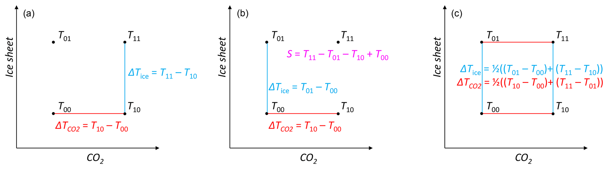
Figure 1Three different factorisation methods of temperature, T, for two variables (CO2 and ice sheets). (a) Linear factorisation, (b) Stein and Alpert (1993) factorisation, (c) Lunt et al. (2012) factorisation. The temperature, T, can be considered as a surface in a third dimension sitting above the two-dimensional plane of CO2 and ice sheets. In Eqs. (1), (3), and (4), and ΔT2=ΔTice.
However, an equally valid linear factorisation would be
and in a non-linear system this would in general give a different answer to Eq. (1). In this sense, the linear factorisation method is not “unique”. However, it is “complete” in the sense that the individual factors sum to the total change (ΔT) exactly, i.e. . Considering the linear factorisation as a “path” starting at T00 and ending at T11, it is also “symmetric”, in that if we instead started from T11 we would retrieve the same numerical values for the two linear factorisations (differing just by a minus sign for the numerical value of each factor). It is also “pure” in that it does not need additional interaction terms (see Sect. 2.2 and 2.3) in order to make it complete.
2.2 The Stein and Alpert (1993) factorisation
Stein and Alpert (1993) proposed an alternative factorisation method, illustrated in Fig. 1b. In this, for the Pliocene case, all four possible simulations are carried out, and the factorisation is performed relative to the pre-industrial case (T00) for all variables. The non-linear terms are then all grouped together in an interaction term (sometimes called the “synergy”), S:
In contrast to the linear factorisation, the Stein and Alpert (1993) factorisation is unique. It is also complete because (in fact, S is defined such that the factoristion is complete). As a result of the interaction term, S, it is not “pure”. In addition, it is not symmetric; if we instead performed the factorisation relative to T11, we would in general obtain a different numerical value of the factorisation (i.e. ).
2.3 The Lunt et al. (2012) factorisation
Lunt et al. (2012) proposed another factorisation, in which the factorisation for a particular variable is defined as the mean of the difference between each pair of simulations that differ by just that variable. This is illustrated in Fig. 1c; the factorisation of ice is represented by the mean of the two blue lines, and the factorisation of CO2 is represented by the mean of the two red lines:
The N=2 factorisation in Eq. (4) is unique, complete, symmetric, and pure. It is worth noting that Eq. (4) can be interpreted in multiple ways – either (i) as described above, the factorisation averages all the possible pairs of simulations that differ solely by a change in that variable (i.e. for a particular variable it is the mean of either the horizontal or vertical edges of the square in Fig. 1c); (ii) it is the average of the two possible linear factorisations in Eqs. (1) and (2); (iii) it is the average of the two possible Stein and Alpert (1993) factorisations obtained by swapping the Pliocene and pre-industrial values (in which case the interaction terms cancel); or (iv) it is the Stein and Alpert (1993) factorisation but with the interaction term, S, shared equally between the two factors.
In extending to N=4 variables, Lunt et al. (2012) assumed that the first of these interpretations would still hold for any number of variables. However, consider the N=3 case illustrated in Fig. 2, in which we have added vegetation as a third variable to contribute to Pliocene warming.
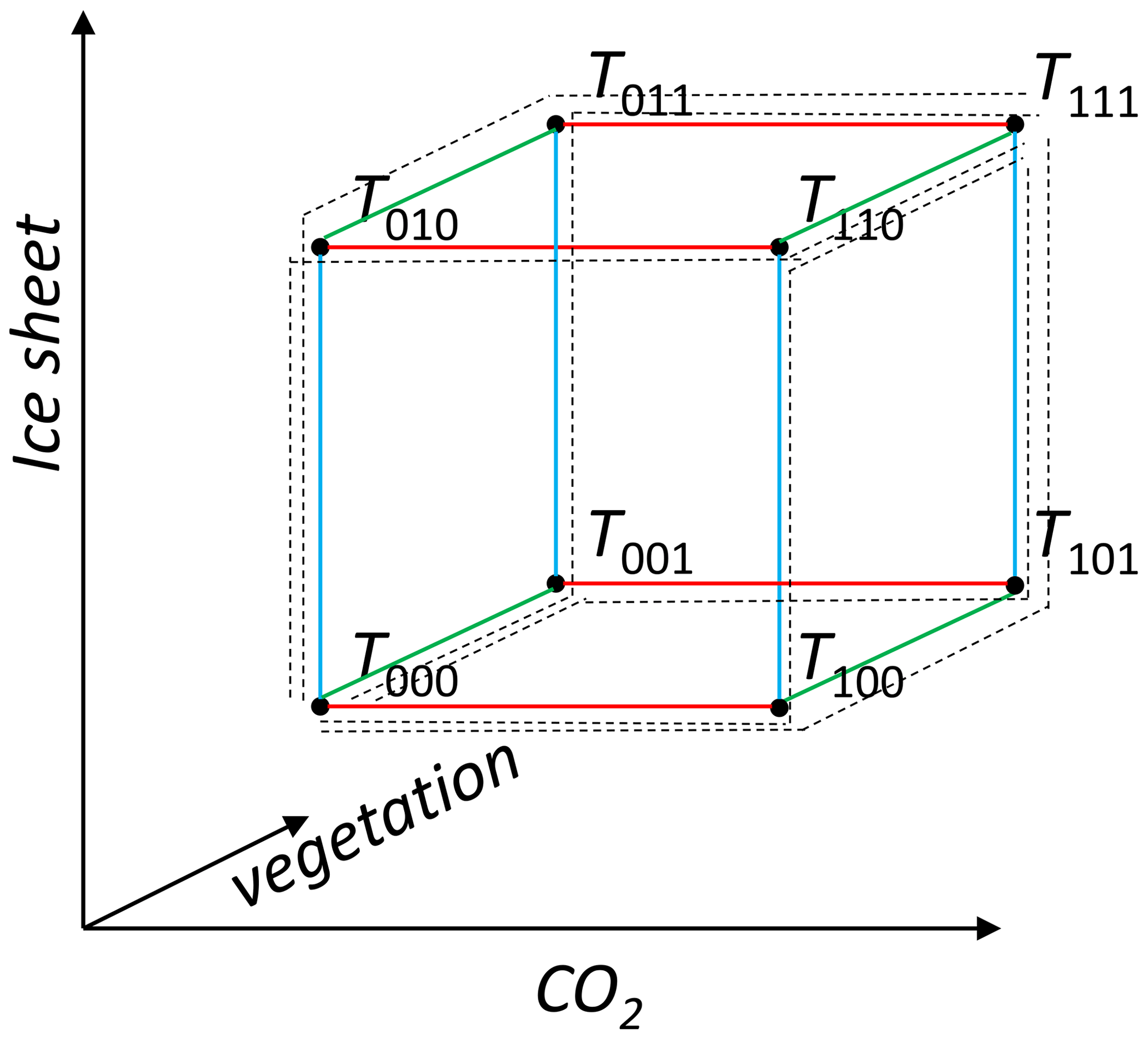
Figure 2Simulations and linear factorisations in an N=3 factorisation. Edges that represent changes in CO2 are in red, changes in ice are in blue, and changes in vegetation are in green. The paths associated with all three possible linear factorisations are shown with dotted lines.
Averaging the edges (interpretation (i) above) would result in a factorisation:
Although this is unique, symmetric, and pure, it is not complete, because . This is apparent by considering the T111 terms; the three lines in Eq. (5) each include a term equal to , which sum to , whereas they are required to sum to T111 for a complete factorisation. As such, an additional interaction term, in the sense of S in Eq. (3), would be required for the factorisation to be complete in N=3 dimensions (in which case it would no longer be pure). Note that the Lunt et al. (2012) factorisation is complete for N=2 without such an interaction term, but this is a case specific to N=2 as a result of cancellation of terms in Eq. (4).
2.4 Summary of previous factorisations
As shown above, neither the linear nor the Stein and Alpert (1993) nor the Lunt et al. (2012) factorisation methods possess all four properties of uniqueness, symmetry, purity, and completeness in N>2 dimensions. These properties are often desirable in a factorisation, because any factorisation that lacks one of these properties is less easy to interpret. For example, for the Pliocene example above, uniqueness means that we can have a single answer to the question “why is the Pliocene warmer than the pre-industrial period”. Symmetry means that we obtain the same answer to the question “why is the Pliocene warmer than the pre-industrial period” as to the question “why is the pre-industrial period colder than the Pliocene”. Completeness means that the answer to the question “how much warmer is the Pliocene than the pre-industrial period” is equal to the sum of the individual factors (plus an interaction term if one exists). “Purity” means that we can answer the question “why is the Pliocene warmer than the pre-industrial period” by referring solely to contributions from our fundamental factors CO2, ice, and vegetation, i.e. without including additional interaction terms that are not attributed to a single factor. These interaction terms are important and interesting, but there are cases where it can be useful or essential to only include attributable terms in the factorisation.
Here we discuss possible extensions to the three previous factorisations discussed above, that are unique, symmetric, pure, and complete in N dimensions.
3.1 Extension to the linear factorisation: the linear-sum factorisation
The linear-sum factorisation arises from a generalisation to N>2 dimensions of the second interpretation of Eq. (4); i.e. it arises from averaging all the possible linear factorisations. This will result in a complete and pure factorisation because each individual linear factorisation is itself complete and pure. For three dimensions, this is illustrated by the dotted lines in Fig. 2.
Each possible linear factorisation can be represented as a non-returning “path” from the vertex T000 to the opposite vertex T111, traversing edges along the way (dotted lines in Fig. 2). When considering the sum of all possible paths, some edges are traversed more than others. In general, those edges near the initial or final vertices are traversed more times than edges that are further away from these vertices. As such, when we average the possible linear factorisations, different edges (corresponding to different terms in the factorisation) will have different weightings. This is in contrast to Eq. (5) where each term (i.e. edge of the cube) has the same weighting. For three dimensions, Fig. 2 shows that the six edges adjacent to the initial and final vertex are traversed twice, whereas the six other edges are traversed only once. Therefore, the factorisation is
This factorisation is complete (), unique, symmetric, and pure.
To generalise to N dimensions, consider an N-dimensional cube, which has a total of 2N vertices and edges. There are 2N−1 edges in each dimension. There are N! paths from the initial vertex of the cube to the final opposite vertex, each of which consists of a traverse along N edges. Therefore, in each dimension there are a total of N! edges traversed for all paths combined.
As for the three-dimensional case above, let us label each vertex, V, of this N-dimensional cube as , where each ai is either 0 or 1. A value ai=0 represents the first value for variable i, and ai=1 represents the second value for variable i. Each vertex is also associated with a system value, denoted (see Fig. 2 for the case N=3).
All factorisations consist of partitioning the total change, between N factors. Each factor is associated with a dimension, i, in the N-dimensional cube. The factorisation for dimension i is ΔTi.
For the linear-sum factorisation, all paths that we consider start at the origin vertex, 0⋯0, and end at the opposite vertex 1⋯1, and they are made up of a series of edges. For all edges on the N-dimensional cube, let us define X as the set of all possible starting vertices, for a given N. For example, for N=3, . Let us define Xi as the set of all possible starting vertices for an edge that is oriented in the ith dimension, i.e. all those vertices that have a 0 in the ith subscript. For example, for N=3 and i=2, . Let us define Yi as the set of all possible ending vertices for an edge that is oriented in the ith dimension, so that Yi is related to Xi by changing the ith subscript of each element from 0 to 1. For example, for N=3 and i=2, . Order Xi and Yi so that their elements correspond. Then we write to indicate the jth element of Xi, and as indicating the jth element of Yi. For example, for the X2 defined above, .
The Lunt et al. (2012) factorisation averages along each edge oriented in dimension i:
For the linear-sum factorisation, we instead carry out a weighted average, with the weight for each edge in dimension i given by how many times it is traversed in all N! paths. Consider all the paths that traverse an edge which starts at a vertex defined by k subscripts of “1” and N−k subscripts of “0”. There are k! possible paths to the start of this edge, and paths from the end of this edge to the final corner (defined by N subscripts of “1”). Therefore, there are paths that use this edge. As such, we can write the linear-sum factorisation as
where is the number of subscripts of “1” in .
For example, for N=4 and i=1, we have N!=24 edges traversed in this dimension, and edges. , and . For those edges with a starting subscript with k=0 subscripts of “1” (i.e. 0000), the weighting . For those edges with a starting subscript with k=1 subscripts of “1” (i.e. ), the weighting . For those edges with a starting subscript with k=2 subscripts of “1” (i.e. ), the weighting . For those edges with a starting subscript with k=3 subscripts of “1” (i.e. 0111), the weighting . Therefore, for N=4 and i=1, we have
3.2 Extension to the Stein and Alpert (1993) factorisation: the shared-interactions factorisation
As stated in Sect. 2.3, the Lunt et al. (2012) factorisation for N=2 can be interpreted as being identical to the Stein and Alpert (1993) factorisation but with the interaction term shared between the two factors (thereby removing the interaction term, resulting in a pure factorisation). Here we explore what happens when this interpretation is generalised to N>2 dimensions. For consistency, we use the same notation as Stein and Alpert (1993). In their notation, represents the difference between a simulation in which only factor i is modified with a simulation in which no factors are modified, and represents interaction terms between the different factors. For example, for our original N=2 example illustrated in Fig. 1 and given in Eq. (3), , , and .
For our Pliocene example for N=3, is the interaction between factors 1 and 2 (CO2 and ice), is the interaction between factors 1 and 3 (CO2 and vegetation), is the interaction between factors 2 and 3 (ice and vegetation), and is the interaction between all three factors. In this case, Stein and Alpert (1993) give that
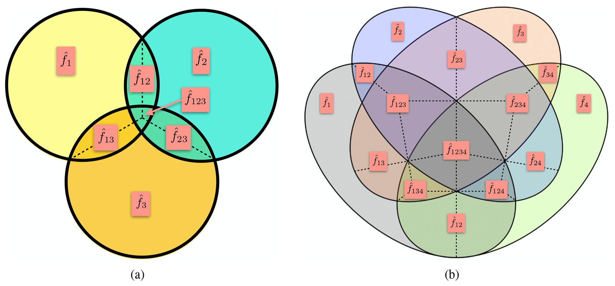
Figure 3(a) Visual representation of the shared-interaction factorisation for N=3, as given by Eq. (10). The straight dotted lines represent the sharing of the interactions according to Eq. (11). (b) Visual representation of the shared-interaction factorisation for N=4. The straight dotted lines represent the sharing of the interactions according to Eq. (13).
As discussed in Sect. 2.2, this factorisation is not symmetric or unique (e.g. we could define ) or pure, but it is complete if we include all the interaction terms, which are not attributed to any particular factor. By extending the interpretation of the shared interaction term in two dimensions discussed in Sect. 2.3, we can choose to share the interaction terms equally between their contributing factors, an approach applied by Schmidt et al. (2010) (although they carried out a fractional factorisation in which not all combinations of all variables were included). This results in a factorisation that is complete and pure (because we are just re-partitioning the interaction terms). It turns out that it is also symmetric. For example for CO2,
This factorisation for N=3 is represented visually in Fig. 3a. Equations (10) and (11) give that, for CO2,
This is identical to the equivalent term in Eq. (6), indicating that the shared-interaction and linear-sum interpretations are identical for N=3, and that therefore for N=3 the shared-interaction factorisation is unique, symmetric, pure, and complete.
Stein and Alpert (1993) give the generalisation of their factorisation to N factors (their Eqs. 11–16). For N=4, the interaction terms are shared so that, for example for CO2,
This factorisation for N=4 is represented visually in Fig. 3b. Again, for N=4 this is identical to the linear-sum interpretation (Eq. 9). We conjecture that for any N these two interpretations will give identical results.
3.3 Extension to the Lunt et al. (2012) factorisation: the scaled-residual factorisation
In the scaled-residual factorisation, the Lunt et al. (2012) factorisation is modified so that it is complete (and remains pure). This is achieved by taking the total residual term required for completeness and sharing this between the factors in proportion to the magnitude of their Lunt et al. (2012) factorisation. For the N=3 example of the Pliocene, we have that the residual term, R, is defined such that
where the values are defined in Eq. (5). We then share this residual proportionally across the three factors, such that
In N dimensions, this is
where is defined in Eq. (7), and
For example, for N=4 and i=1 we have
and the same applies to , , and .
Here we discuss three examples of papers in which the Lunt et al. (2012) factorisation has been used. For each, we show how using our factorisations would affect the results in that paper.
4.1 Implications for Lunt et al. (2012)
Lunt et al. (2012) presented a factorisation of global mean temperature change in the Pliocene into four variables: CO2, orography, ice, and vegetation. As described in Sect. 2.3, in extending to N=4 variables, the Lunt et al. (2012) factorisation is unique, symmetric, and pure, but not complete. Using their notation, their factorisation for the CO2 variable is (equivalent to Eq. 9 in their paper)
The equivalent linear-sum/shared-interaction factorisation is given by Eq. (9), which in the notation of Lunt et al. (2012) is
and similarly for the other three variables.
The equivalent scaled-residual factorisation is given by Eq. (18), which in the notation of Lunt et al. (2012) is
where is given in Eq. (19), and the same applies to the other three variables.
In Lunt et al. (2012), although Eq. (19) (Eq. 9 in their paper) was presented, the four variables were actually factorised by two N=2 factorisations for all the analysis in that paper (Eq. 13 in their paper). Because for N=2 dimensions the Lunt et al. (2012), linear-sum/shared-interaction, and scaled-residual factorisations are identical, the actual results related to Pliocene temperature change presented in Lunt et al. (2012) would not be affected by using our proposed new factorisations.
4.2 Implications for Haywood et al. (2016)
Haywood et al. (2016), in the context of the experimental design for model simulations of the Pliocene in the PlioMIP project, presented a three-variable factorisation of Pliocene warming into components due to CO2, topography, and ice, based on the Lunt et al. (2012) factorisation (presented in their Sect. 3.2).
An alternative, using the linear-sum/shared-interaction factorisation that is complete, is obtained from Eq. (6), which in their notation is, for CO2 (and analogously for the other two components),
Another alternative, using the scaled-residual factorisation that is complete, is obtained from Eqs. (14) and (15), which in their notation is, for CO2 (and analogously for the other two components),
4.3 Implications for Chandan and Peltier (2018)
Chandan and Peltier (2018) applied the N=3 factorisation of Lunt et al. (2012) (Eq. 5), as also given by Haywood et al. (2016) (first line of Eq. 23), to their suite of Pliocene simulations. The factorisation was applied to each grid cell in the model, resulting in 296 factorisations over the globe. The two-dimensional mid-Pliocene minus pre-industrial temperature anomaly, reproduced here in Fig. 4a, was factorised into contributions originating from a change in CO2, orography and ice sheets. Figure 4b–d show the results of the original factorisation and are identical to those presented in Fig. 7 of Chandan and Peltier (2018). Figure 4f–h show the factorisation of the same anomaly using the linear-sum/shared-interaction method (Eq. 22), while Fig. 4j–m show the results of employing the scaled-residual method (Eq. 23). The first thing to note is that the three factorisations all have very similar results; visually it is difficult to tell them apart on a regional scale, and they result in global means for each factor that differ by less than 10 %. This is because, in this example, the non-linearities (i.e. the interaction terms) are relatively small. As such, the main conclusions of the Chandan and Peltier (2018) study are robust to a change in factorisation methodology.

Figure 4Comparison of various factorisation methods. (a) The mid-Pliocene minus pre-industrial anomaly (T111−T000) modelled by Chandan and Peltier (2017). (b–m) The top three rows present factorisations of the total anomaly into contributions arising from changes to CO2 (upper, b, f, j), orography (middle, c, g, k), and ice sheets (lower, d, h, l), while the bottom row shows the residual required for completeness (e, i, m). Note that the residual term, R, for panel (e) is given by Eq. (14) and is equal to . The first column (b, c, d, e) shows results using the methodology of Lunt et al. (2012) and is identical to results reported in Fig. 7 of Chandan and Peltier (2018). The second column (f, g, h, i) shows results from the linear-sum/shared-interaction factorisation (Eq. 6), and the third column (j, k, l, m) shows results of the scaled-residual factorisation (Eq. 15). The values at the top-right of each panel give the global mean, in units of ∘C.
Table 1Properties of the factorisations discussed in this paper.

* For these properties, we show that the properties hold for the linear-sum factorisation for N factors and conjecture that the linear-sum and shared-interaction factorisations are identical.
The bottom row in Fig. 4 shows, for the case of each method, the residual difference between the sum of all the factors and the total change (i.e. the interaction/synergy terms in the sense of Stein and Alpert, 1993). The Lunt et al. (2012) method yields spatially coherent structures in the residual whose magnitude can be comparable to those of the factorised components, whereas the residuals for the other two methods are zero by definition, because they are pure (in the figures they are very close to zero – essentially numerical noise due to round-off error). The non-linearity (indicated by the magnitude of the residual term associated with the Lunt et al. (2012) factorisation) is greatest in the North Atlantic (Fig. 4d) and is likely associated with changes in the sea-ice margin that are non-linearly influenced by all three boundary conditions (CO2, orography, and ice sheets).
We also explored using a version of the scaled-residual factorisation in which the residual terms were shared, not by the absolute magnitude of the individual factors, but by their relative values, so that Eq. (15) became
and similarly for the other variables. However, at a small number of grid cells this produced highly divergent results, when the denominator in Eq. (24) became very close to zero (see Supplement Fig. S1).
In this paper, we have reviewed three previously proposed factorisations and extended them to produce factorisations that are unique, symmetric, pure, and complete. We have presented them for three dimensions (i.e. three factors) and generalised to N dimensions. The first factorisation, “linear-sum” (Eq. 8), averages all the possible linear factorisations on the N-dimensional cube. The second factorisation, “shared-interaction”, shares the interaction terms between each corresponding factor equally. The linear-sum and shared-interaction factorisations are shown to reduce to be identical for N≤4, and we conjecture that this holds for any N. The third factorisation, “scaled-residual” (Eq. 16), takes the residual term required for completeness in the Lunt et al. (2012) factorisation and shares it between the factors, in proportion to their magnitude. We have presented results of these extended factorisations in the context of previous work carried out by Lunt et al. (2012), Haywood et al. (2016), and Chandan and Peltier (2018) in the context of Pliocene climate change. We recommend the use of the linear-sum/shared-interaction factorisation or the scaled-residual factorisation for cases where the properties of uniqueness, symmetry, purity, and completeness are desirable. In some cases, the interaction terms may, of course, be of great interest, and in such cases a non-pure factorisation (e.g. Stein and Alpert, 1993) can be very informative. Also, it is worth noting that if the interaction terms are zero, i.e. we have a completely linear system, then all the factorisation methods reduce to be identical. The properties of all the factorisations discussed in this paper are shown in Table 1 for and N dimensions.
The methods that we present here will be of particular use in the analysis of systems with multiple variables and are applicable beyond solely climate science.
The model fields underlying Fig. 4 are available from the University of Toronto Dataverse in NetCDF format: https://doi.org/10.5683/SP2/QGK5B0 (Chandan, 2020). The code used to calculate the factorisations illustrated in Fig. 4 is available in the Supplement, in both Python and NCL. They are also available on GitHub at https://github.com/danlunt1976/factor_separation/blob/master/factor_separation.ncl (last access: 2 July 2021) and at https://github.com/danlunt1976/factor_separation/blob/master/factorize_gmd.py (last access: 2 July 2021).
The supplement related to this article is available online at: https://doi.org/10.5194/gmd-14-4307-2021-supplement.
DJL led the study and wrote the first draft of the paper. GAS made Fig. 3 and DC made Fig. 4. DJL devised the linear-sum factorisation, GAS devised the shared-interaction factorisation, and GML devised the scaled-residual factorisation. JCR provided the derivation of Eq. (8). US, PJV, and AMH developed the boundary conditions and early Pliocene modelling that underpin the Pliocene simulations discussed. All authors contributed to writing the final version of the paper.
The authors declare that they have no conflict of interest.
Publisher's note: Copernicus Publications remains neutral with regard to jurisdictional claims in published maps and institutional affiliations.
The authors are grateful to Harry J. Dowsett for developing the boundary conditions that underpin the Pliocene simulations discussed.
This research has been supported by NERC (grant no. NE/P01903X/1).
This paper was edited by James Annan and reviewed by Chris Brierley and one anonymous referee.
Alpert, P. and Sholokhman, T. (Eds.): Factor Separation in the Atmosphere: Applications and Future Prospects, Cambridge University Press, https://doi.org/10.1017/CBO9780511921414, 2011. a
Box, G. E. P., Hunter, J. S., and Hunter, W. G.: Statistics for Experimenters, 2nd Edn., John Wiley and Sons, 2005. a
Burke, K. D., Williams, J. W., Chandler, M. A., Haywood, A. M., Lunt, D. J., and Otto-Bliesner, B. L.: Pliocene and Eocene provide best analogs for near-future climates, P. Natl. Acad. Sci. USA, 115, 13288–13293, https://doi.org/10.1073/pnas.1809600115, 2018. a
Chandan, D.: Pliocene surface temperature data for Multi-variate factorisation methods, Scholars Portal Dataverse, V1, https://doi.org/10.5683/SP2/QGK5B0, 2020. a
Chandan, D. and Peltier, W. R.: Regional and global climate for the mid-Pliocene using the University of Toronto version of CCSM4 and PlioMIP2 boundary conditions, Clim. Past, 13, 919–942, https://doi.org/10.5194/cp-13-919-2017, 2017. a
Chandan, D. and Peltier, W. R.: On the mechanisms of warming the mid-Pliocene and the inference of a hierarchy of climate sensitivities with relevance to the understanding of climate futures, Clim. Past, 14, 825–856, https://doi.org/10.5194/cp-14-825-2018, 2018. a, b, c, d, e
Claussen, M., Brovkin, V., and Ganopolski, A.: Biogeophysical versus biogeochemical feedbacks of large-scale land cover change, Geophys. Res. Lett., 28, 1011–1014, https://doi.org/10.1029/2000GL012471, 2001. a
Domagni, K. F., Hedayat, A., and Sinha, B. K.: On the nature of saturated 2k- factorial designs for unbiased estimation of non-negligible parameters, J. Stat. Plan. Infer., 211, 33–40, https://doi.org/10.1016/j.jspi.2020.05.006, 2021. a
Dowsett, H., Dolan, A., Rowley, D., Moucha, R., Forte, A. M., Mitrovica, J. X., Pound, M., Salzmann, U., Robinson, M., Chandler, M., Foley, K., and Haywood, A.: The PRISM4 (mid-Piacenzian) paleoenvironmental reconstruction, Clim. Past, 12, 1519–1538, https://doi.org/10.5194/cp-12-1519-2016, 2016. a
Fisher, R. A.: The arrangement of field experiments, Journal of the Ministry of Agriculture of Great Britain, 33, 503–513, 1926. a
Haywood, A. M., Dowsett, H. J., Dolan, A. M., Rowley, D., Abe-Ouchi, A., Otto-Bliesner, B., Chandler, M. A., Hunter, S. J., Lunt, D. J., Pound, M., and Salzmann, U.: The Pliocene Model Intercomparison Project (PlioMIP) Phase 2: scientific objectives and experimental design, Clim. Past, 12, 663–675, https://doi.org/10.5194/cp-12-663-2016, 2016. a, b, c, d
Haywood, A. M., Tindall, J. C., Dowsett, H. J., Dolan, A. M., Foley, K. M., Hunter, S. J., Hill, D. J., Chan, W.-L., Abe-Ouchi, A., Stepanek, C., Lohmann, G., Chandan, D., Peltier, W. R., Tan, N., Contoux, C., Ramstein, G., Li, X., Zhang, Z., Guo, C., Nisancioglu, K. H., Zhang, Q., Li, Q., Kamae, Y., Chandler, M. A., Sohl, L. E., Otto-Bliesner, B. L., Feng, R., Brady, E. C., von der Heydt, A. S., Baatsen, M. L. J., and Lunt, D. J.: The Pliocene Model Intercomparison Project Phase 2: large-scale climate features and climate sensitivity, Clim. Past, 16, 2095–2123, https://doi.org/10.5194/cp-16-2095-2020, 2020. a
Hogrefe, C., Lynn, B., Civerolo, K., Ku, J.-Y., Rosenthal, J., Rosenzweig, C., Goldberg, R., Gaffin, S., Knowlton, K., and Kinney, P. L.: Simulating changes in regional air pollution over the eastern United States due to changes in global and regional climate and emissions, J. Geophys. Res.-Atmos., 109, D22301, https://doi.org/10.1029/2004JD004690, 2004. a
Lunt, D. J., Haywood, A. M., Schmidt, G. A., Salzmann, U., Valdes, P. J., Dowsett, H. J., and Loptson, C. A.: On the causes of mid-Pliocene warmth and polar amplification, Earth Planet. Sc. Lett., 321–322, 128–138, https://doi.org/10.1016/j.epsl.2011.12.042, 2012. a, b, c, d, e, f, g, h, i, j, k, l, m, n, o, p, q, r, s, t, u, v, w, x, y, z, aa
McClymont, E. L., Ford, H. L., Ho, S. L., Tindall, J. C., Haywood, A. M., Alonso-Garcia, M., Bailey, I., Berke, M. A., Littler, K., Patterson, M. O., Petrick, B., Peterse, F., Ravelo, A. C., Risebrobakken, B., De Schepper, S., Swann, G. E. A., Thirumalai, K., Tierney, J. E., van der Weijst, C., White, S., Abe-Ouchi, A., Baatsen, M. L. J., Brady, E. C., Chan, W.-L., Chandan, D., Feng, R., Guo, C., von der Heydt, A. S., Hunter, S., Li, X., Lohmann, G., Nisancioglu, K. H., Otto-Bliesner, B. L., Peltier, W. R., Stepanek, C., and Zhang, Z.: Lessons from a high-CO2 world: an ocean view from ∼ 3 million years ago, Clim. Past, 16, 1599–1615, https://doi.org/10.5194/cp-16-1599-2020, 2020. a
Montgomery, D. C.: Design and Analysis of Experiments, John Wiley & Sons, Inc), ISBN 978-1-118-14692-7, 8th Edn., 724 pp., 2013. a, b
Schmidt, G. A., Ruedy, R., Miller, R. L., and Lacis, A. A.: The attribution of the present-day total greenhouse effect, J. Geophys. Res., 115, D20106, https://doi.org/10.1029/2010JD014287, 2010. a, b
Smucker, B., Krzywinski, M., and Altman, N.: Two-level factorial experiments, Nature Methods, 16, 211–212, https://doi.org/10.1038/s41592-019-0335-9, 2019. a
Stein, U. and Alpert, P.: Factor separation in numerical simulations, J. Atmos. Sci., 50, 2107–2115, 1993. a, b, c, d, e, f, g, h, i, j, k, l, m, n, o, p
van den Heever, S. C., Carrió, G. G., Cotton, W. R., DeMott, P. J., and Prenni, A. J.: Impacts of Nucleating Aerosol on Florida Storms. Part I: Mesoscale Simulations, J. Atmos. Sci., 63, 1752–1775, https://doi.org/10.1175/JAS3713.1, 2006. a
- Abstract
- Introduction
- Previous factorisation methods
- Extensions to the previous factorisations
- Implications for previous published work
- Conclusions
- Code and data availability
- Author contributions
- Competing interests
- Disclaimer
- Acknowledgements
- Financial support
- Review statement
- References
- Supplement
swapping in and outdifferent values of these factors, and can also carry out experiments with many different combinations of these factors. This paper discusses how best to analyse the results from such experiments.
- Abstract
- Introduction
- Previous factorisation methods
- Extensions to the previous factorisations
- Implications for previous published work
- Conclusions
- Code and data availability
- Author contributions
- Competing interests
- Disclaimer
- Acknowledgements
- Financial support
- Review statement
- References
- Supplement