the Creative Commons Attribution 4.0 License.
the Creative Commons Attribution 4.0 License.
 | 05 Jul 2021
Inclusion of a suite of weathering tracers in the cGENIE Earth system model – muffin release v.0.9.23
Andy Ridgwell
Fanny M. Monteiro
Ian J. Parkinson
Alexander J. Dickson
Philip A. E. Pogge von Strandmann
Matthew S. Fantle
Sarah E. Greene
The metals strontium (Sr), lithium (Li), osmium (Os) and calcium (Ca), together with their isotopes, are important tracers of weathering and volcanism – primary processes which shape the long-term cycling of carbon and other biogeochemically important elements at the Earth's surface. Traditionally, because of their long residence times in the ocean, isotopic shifts in these four elements observed in the geologic record are almost exclusively interpreted with the aid of isotope-mixing, tracer-specific box models. However, such models may lack a mechanistic description of the links between the cycling of the four metals to other geochemically relevant elements, particularly carbon, or climate. Here we develop and evaluate an implementation of Sr, Li, Os and Ca isotope cycling in the Earth system model cGENIE. The model offers the possibility to study the dynamics of these metal systems alongside other more standard biogeochemical cycles, as well as their relationship with changing climate. We provide examples of how to apply this new model capability to investigate Sr, Li, Os and Ca isotope dynamics and responses to environmental change, for which we take the example of massive carbon release to the atmosphere.
- Article
(5766 KB) - Full-text XML
-
Supplement
(87 KB) - BibTeX
- EndNote


The evolution of life and climate on Earth is intrinsically linked to the dynamics of carbon, oxygen and nutrients at the Earth's surface. While complex interactions on a range of spatial and temporal scales determine the distribution of these elements between surficial (non-lithological) reservoirs like oceans, atmosphere, biomass and soils, the total amount and isotopic distribution of these elements is ultimately governed by the balance between crustal weathering, marine sediment deposition and mantle inputs associated with oceanic crust formation. The geological record shows that the abundance of these elements at Earth's surface has varied on timescales of thousands to millions of years. For example, the changing composition of mantle fluxes into the ocean and nutrient supply during weathering of large mountain ranges were potentially drivers of the accumulation of surficial oxygen during the Archean and Proterozoic (e.g., Kump and Barley, 2007; Campbell and Allen, 2008). Increased basalt weathering in the Cenozoic could have led to a continuous decline in CO2 concentrations, contributing to the reconstructed long-term cooling trend (e.g., Kent and Muttoni, 2013; Mills et al., 2014) while the emplacement of large igneous provinces (LIPs) repeatedly led to climatic and biotic crises by increasing the supply of mantle-derived carbon and nutrients to the oceans, e.g., during oceanic anoxic events (e.g., Erba et al., 2010; Jenkyns, 2010; Bottini et al., 2012; Monteiro et al., 2012; Percival et al., 2015). At the other (late Quaternary) end of the geological timescale, the supply of particulate iron from airborne ground rock to the oceans of the Quaternary has been invoked as a mechanism to drive glacial–interglacial carbon cycle dynamics (e.g., Martin, 1990; Martínez-Garcia et al., 2011; Loveley et al., 2017; Hooper et al., 2019), linking erosion of the land surface, trace metal cycles in the ocean, and atmospheric pCO2 (Ridgwell and Watson, 2002).
Understanding mass fluxes between the lithosphere and Earth's dynamic surface are thus key to understanding climate change over geological timescales. However, past changes cannot be reconstructed directly. Instead, variations in the oceanic content and isotopic composition of trace metals like strontium (Sr), osmium (Os), lithium (Li) and calcium (Ca) preserved in marine sediments are used to study lithological processes. The dynamics of these metals are controlled by processes that also shape the long-term carbon and nutrient cycles, namely continental and oceanic weathering and direct mantle emissions, and variations in their isotopic compositions can be linked more directly to changes in these processes since radioactive decay and mass-dependent fractionation form isotopically distinct lithological metal reservoirs. Furthermore, the long residence time of these metals in the ocean, which is generally assumed to be greater than the mixing time of the ocean, generally removes the complexity of spatially heterogeneous marine records since their marine distribution is comparably homogeneous (e.g., Faure and Mensing, 2005), and marine sedimentary records are typically understood as capturing global signals.
Despite laboratory methods to measure and reconstruct the evolving trace metal composition of seawater have become increasingly precise, our ability to interpret these records is limited by our incomplete mechanistic understanding of the cycling of these metals and their isotopes. Mass balances and box models have been most commonly used to interpret geological records of trace metal variations (e.g., Tejada et al., 2009; Misra and Froelich, 2012; Kristall et al., 2017; Them et al., 2017). However, they cannot mechanistically resolve spatially heterogeneous metal burial, and hence they often rely on assumed global fluxes and residence times based on today's ocean, which might not always be applicable throughout the geological record. Additionally, they tend not to include effects of Earth system feedbacks (e.g., climate-driven weathering flux changes, sediment dissolution), the simulation of which requires information about spatially heterogeneous climate and ocean variables, bathymetry, and continental configuration. In contrast, more mechanistic and spatially resolved Earth system models of intermediate complexity (EMIC) aim to capture spatial heterogeneity in marine sources and sinks while making numerical compromises elsewhere (such as in omitting atmospheric dynamics). Of relevance here, the EMIC “cGENIE” has been used successfully to study marine biogeochemical cycles (including C and Ca) under various boundary conditions and external forcings (e.g., Ridgwell and Zeebe, 2005; Ridgwell et al., 2007; John et al., 2014; Death et al., 2014; Turner and Ridgwell, 2016; Hülse e al., 2019). Adding a mechanistic description of the cycling of Sr, Os, Li and Ca (plus isotopes) in cGENIE thus allows us to test their behavior under environmental perturbations alongside nutrient, redox and carbon dynamics (plus climate change) and to compute their spatial distributions and marine residence times under different assumptions about source and sink mechanisms.
Here, we present an implementation of the marine cycling of Sr, Os, Li and Ca in cGENIE. We evaluate the model's performance by comparing simulations of pre-industrial trace metal distributions in the oceans to seawater measurements and study their equilibration times under imposed geochemical perturbations compared to established seawater residence times.
We first provide a brief review of Sr, Os, Li and Ca cycling in the ocean (Sect. 2.1–2.4), as well as their observed concentrations and isotopic compositions in seawater (Sect. 2.5) and their applications as proxies for Earth system processes (Sect. 2.6).
2.1 Strontium
Of the four metal cycles simulated in this study, Sr has the second-highest marine concentration (3 to 4 times more abundant than Li and more than a billion times more abundant than Os, Angino et al., 1966). The main source for marine Sr is continental weathering, replenishing the ocean reservoir through rivers and potentially groundwater discharge (Basu et al., 2001; Beck et al., 2013). Smaller sources include hydrothermal input of mantle-derived Sr and refluxes from diagenetic alteration of carbonates at the seafloor. The chemical and physical similarity of Sr to Ca leads to its substitution in aragonite and, to a lesser degree, calcite (Fietzke and Eisenhauer, 2006; Rüggeberg et al., 2008; Böhm et al., 2012; Stevenson et al., 2014). Angino et al. (1966) argue that biological uptake is the dominant driver of spatial gradients in Sr concentrations in today's oceans, and Krabbenhöft et al. (2010) predict that marine carbonate burial could be the most important sink of seawater Sr. The concentration of Sr incorporated into biogenic carbonates depends on the mineralogy and the growth rate with higher ratios in aragonite precipitated at fast growth rates (Rickaby et al., 2002; Stevenson et al., 2014). In contrast, direct effects of temperature on elemental fractionation during the formation of calcite, the major carbonate buried in marine sediments, are small (Tang et al., 2008). Assuming rivers to be the only supply of continental Sr to the oceans and that the marine Sr reservoir size is in equilibrium, Hodell et al. (1989) estimate the marine residence time of Sr to be 1.9–3.45 Myr. Considering the potentially appreciable Sr influx from groundwater, the actual residence time might be at or below the lower end of this estimate, and it may be even more different if the marine Sr reservoir is not currently in equilibrium with Sr inputs, as suggested by, e.g., Vance et al. (2009).
Strontium has four stable isotopes (0.56 % 84Sr, 9.87 % 86Sr, 7.04 % 87Sr, 82.53 % 88Sr) (Veizer, 1989), 87Sr being the product of β decay of 87Rb (half-life 4.88×10¹⁰ years, Faure and Mensing, 2005). Radiogenic Sr isotope ratios are reported as ratios, whereas stable Sr isotope ratios are reported as , which is the per mill (‰) deviation in the relative to the NBS987 standard (, Fietzke and Eisenhauer, 2006). Elemental fractionation during magmatic processes creates different ratios that over time generate reservoirs with distinct Sr isotopic signatures, with the continental crust being considerably more radiogenic than the mantle (Faure and Mensing, 2005). Dust and rainwater isotopic signatures, both radiogenic and stable, are generally lower than modern-day seawater values (Pearce et al., 2015). Volcanic material brings un-radiogenic particulate Sr into sediments and can over time significantly affect the radiogenic composition of dissolved Sr in the sediment column while having little effect on the isotopic composition of dissolved Sr in seawater (Elderfield and Gieskes, 1982; Pearce et al., 2015). Changes in isotope abundances caused by kinetic and equilibrium mass-dependent fractionation during carbonate formation are much smaller, and one can thus assume that the of seawater and deposited carbonates is only controlled by inputs to the ocean (Krabbenhöft, 2011). By contrast, variations in Sr are only controlled by fractionation during chemical processes, biogenic carbonate formation being the most important one in the ocean (e.g., Krabbenhöft et al., 2010). There is no evidence for a general dependence of Sr fractionation during biogenic carbonate formation on environmental conditions, although temperature and growth rate effects were observed in some calcifying species (Fietzke and Eisenhauer, 2006; Böhm et al., 2012; Stevenson et al., 2014; Vollstaedt et al., 2014).
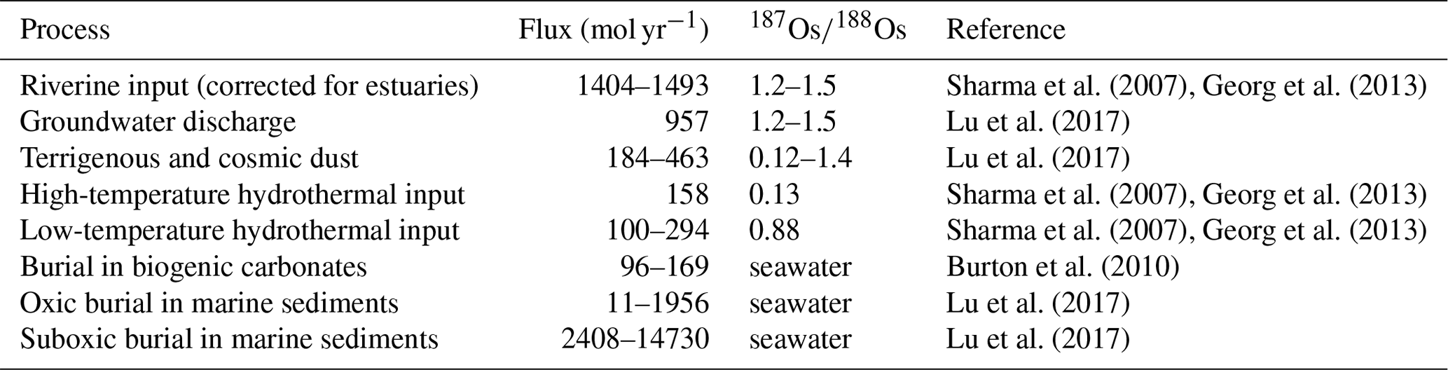
A list of the different sources and sinks of Sr, together with flux estimates and isotopic values, is given in Table 1. The Sr cycle is also summarized in Fig. 2.
Pearce et al. (2015)Kristall et al. (2017)Kristall et al. (2017)Allègre et al. (2010)Peucker-Ehrenbrink et al. (2010)Pearce et al. (2015)Kristall et al. (2017)Allègre et al. (2010)Peucker-Ehrenbrink et al. (2010)Kristall et al. (2017)Basu et al. (2001)Beck et al. (2013)Pearce et al. (2015)Krabbenhöft et al. (2010)Stevenson et al. (2014)Kristall et al. (2017)Krabbenhöft et al. (2010)Menzies and Seyfried (1979)Kristall et al. (2017)Table 1Estimates of pre-industrial Sr fluxes between surface reservoirs and their isotopic composition.

2.2 Osmium
Osmium, a siderophile (affinity for iron) and chalcophile (affinity for sulfur) element, is compatible during mantle melting and as such is accumulated in Earth's core (Goldschmidt, 1922). As a result, it is one of the rarest elements in the Earth's crust and the oceans. Because of its low concentrations, the ability to measure Os in seawater was only developed in the past few decades, limiting the number of observations of marine Os concentrations and isotopic compositions.
The cycling of Os at the Earth's surface is similar to that of radiogenic Sr in many aspects. Oxidative weathering of sediments exposed at the land surface is currently the most important natural source of Os to the oceans (Peucker-Ehrenbrink and Ravizza, 2000; Lu et al., 2017). The estimated annual input of such Os to the oceans via aeolian and riverine transport and groundwater discharge is about 5 times larger than all other natural inputs combined (Lu et al., 2017). Hydrothermal inputs constitute the next largest source of oceanic Os, with high- and low-temperature systems being of roughly equal importance (Georg et al., 2013). The high-temperature hydrothermal source can be split into a basaltic and a peridotitic source (Burton et al., 2010). Unlike for Sr, cosmic and terrestrial dust are significant sources of marine Os (Sharma et al., 2007). Os is removed from the ocean by deposition at the seafloor, predominantly under suboxic conditions and in association with organic matter, and in ferro-manganese nodules (Lu et al., 2017). Os incorporation into biogenic carbonates constitutes an additional but minor sink (Burton et al., 2010). The marine residence time of Os is inherently uncertain given the uncertainty in Os fluxes. Estimates range from 3–50 kyr (Sharma et al., 1997; Levasseur et al., 1998; Oxburgh, 2001).
Os has seven naturally occurring isotopes (0.02 % 184Os, 1.59 % 186Os, 1.51 % 187Os, 13.29 % 188Os, 16.22 % 189Os, 26.38 % 190Os, 40.98 % 192Os). 186Os has such a long half-life that it can also be treated as stable over geologic time, whereas 187Os is radiogenic due to the β decay of 187Re (Faure and Mensing, 2005). The isotopic composition of Os in marine sediments provides insight into changing fluxes between different Os reservoirs, particularly weathering-related Os fluxes from the continents and mantle-derived fluxes from volcanic activity. During partial melt in the upper mantle, Os is more compatible than rhenium (Re), leading to an increased ratio in continental crust relative to the mantle (Dąbek and Halas, 2007) and therefore elevated ratios in the continental crust compared to the mantle. No isotopic fractionation has been observed during Os uptake into macroalgae (Racionero-Gómez et al., 2017), nor is it assumed to occur during other transfers between surface reservoirs.
A list of the different sources and sinks of Os together with flux estimates and isotopic values is given in Table 2. The Os cycle is also summarized in Fig. 2.
Sharma et al. (2007)Georg et al. (2013)Lu et al. (2017)Lu et al. (2017)Sharma et al. (2007)Georg et al. (2013)Sharma et al. (2007)Georg et al. (2013)Burton et al. (2010)Lu et al. (2017)Lu et al. (2017)Table 2Estimates of pre-industrial Os fluxes between surface reservoirs and their isotopic composition. In the calculation of Os burial with Ca carbonate, the estimates of Ca burial in Table 4 were used.
2.3 Lithium
Lithium is the 25th most abundant element in the Earth's crust, and it is more concentrated in continental crust than in oceanic crust (Baskaran, 2011). Weathering, in particular of silicate rocks, releases dissolved Li to rivers and soils where it is partially removed and bound during clay formation (Kısakűrek et al., 2005; Dellinger et al., 2015; Pogge von Strandmann et al., 2017). The remaining dissolved Li is transported to the oceans via rivers and groundwater. Aeolian transport only contributes a minor flux of Li to the oceans (Baskaran, 2011). Li is also added to the oceans by hydrothermal vents and submarine weathering, but the size of this flux is more uncertain (Chan et al., 1992; Hathorne and James, 2006). Removal from the ocean happens predominantly via Li adsorption onto clay minerals, with a minor proportion buried as Li-containing biogenic calcite (Hathorne and James, 2006). These removal fluxes are dependent on the abundance of inorganic carbon and pH (or carbonate saturation) (Hall and Chan, 2004; Marriott et al., 2004) and are not spatially uniform (Hathorne and James, 2006). The residence time of Li in the ocean is estimated to be 0.3–3 Myr (Stoffyn-Egli and Mackenzie, 1984) with more recent estimates closer to 1 Myr (Vigier and Goddéris, 2015).
Li has two stable isotopes (7.52 % 6Li and 92.48 % 7Li, Penniston-Dorland et al., 2017). The isotopic composition of Li is expressed as δ7Li, which is the ‰ deviation of the ratio from the L-SVEC standard (). While earlier studies suggested considerable spatial variability in seawater δ7Li (Carignan et al., 2004), more recent studies suggest that seawater is remarkably homogeneous in its δ7Li (Hall et al., 2005; Rosner et al., 2007; Penniston-Dorland et al., 2017) consistent with its long residence time. Isotope fractionation has been observed during clay formation, adsorption onto minerals and incorporation of Li into calcite shells (Pistiner and Henderson, 2003; Rudnick et al., 2004; Dellinger et al., 2015; Hindshaw et al., 2019) in magmatic systems (Parkinson et al., 2007; Penniston-Dorland et al., 2017), as well as potentially in aqueous solutions (Richter et al., 2006). Isotopic differences in weathered lithologies and post-weathering formation of secondary minerals in rivers and soils result in large spatial and temporal variability of the δ7Li of continental runoff (Huh et al., 1998; Pistiner and Henderson, 2003; Dellinger et al., 2015; Pogge von Strandmann and Henderson, 2015). Temporal variations in the amount of secondary mineral formation on land have the potential to drive shifts in seawater δ7Li over geological time (Misra and Froelich, 2012; Pogge von Strandmann and Henderson, 2015). Fractionation during biogenic carbonate formation results in carbonate δ7Li values that are a few per mill lower than seawater, but this offset seems to be carbonate producer dependent (Hathorne and James, 2006).
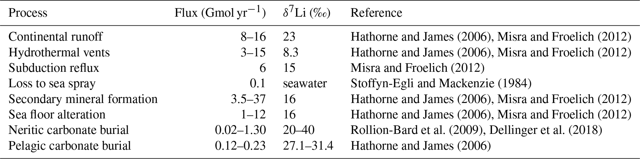
A list of the different sources and sinks of Li, together with flux estimates and isotopic values, is given in Table 3. The Li cycle is also summarized in Fig. 2.
Hathorne and James (2006)Misra and Froelich (2012)Hathorne and James (2006)Misra and Froelich (2012)Misra and Froelich (2012)Stoffyn-Egli and Mackenzie (1984)Hathorne and James (2006)Misra and Froelich (2012)Hathorne and James (2006)Misra and Froelich (2012)Rollion-Bard et al. (2009)Dellinger et al. (2018)Hathorne and James (2006)Table 3Estimates of pre-industrial Li fluxes between surface reservoirs and their isotopic composition. In the calculation of Li burial with calcium carbonate, the estimates of calcium burial in Table 4 were used, assuming a 50:50 split in calcium carbonate burial fluxes between neritic and pelagic environments (Milliman, 1993).
2.4 Calcium
Calcium cycling is closely linked to the C cycle, both shaping and shaped by the size of C reservoirs and C fluxes at the Earth's surface. Similar to Sr, Os and Li, the dominant Ca source for today's oceans is weathering-derived dissolved and particulate Ca in continental runoff. Input through hydrothermal vents near ocean ridges is on the order of 20 % of the riverine flux (e.g., Milliman, 1993; DePaolo, 2004). Unlike Sr, Os and Li, Ca plays an important role in many biological systems, predominantly as an electrolyte and building block for biogenic minerals (e.g., shells, exoskeletons, bones and teeth). In the ocean, Ca ions are incorporated into biogenic minerals (e.g., foraminiferal tests and calcareous nannoplankton), or form hydrogenetic or authigenic minerals (Fantle et al., 2020) if waters are highly saturated (). The resulting minerals will tend to be dissolved in undersaturated conditions or buried, compacted and lithified under saturated conditions. Carbonate formation creates the biggest long-term Ca and C sinks in today's oceans, and marine carbonate accumulation and dissolution constitute a significant buffer mechanism to stabilize marine and atmospheric pCO2 during periods of enhanced exogenic C input (see Ridgwell and Zeebe, 2005). The residence time of Ca in seawater is estimated to be 0.5–1.3 million years (Milliman, 1993; Sime et al., 2007; Griffith et al., 2008).
Ca has 6 stable isotopes (96.941 % 40Ca, 0.647 % 42Ca, 0.135 % 43Ca, 2.086 % 44Ca, 0.004 % 46Ca, 0.187 % 48Ca). 48Ca has such a long half-life that it can be treated as a stable isotope, whereas a small component of the 40Ca in a rock mineral is radiogenic (via decay of 40K; Ga) and accumulates in continental crust over geological timescales (Fantle and Tipper, 2014). The isotopic composition of Ca is reported as either or Ca, which are the ‰ deviations in and Ca, respectively, from NIST SRM-915a, SRM-915b, or modern seawater (see Fantle and Tipper, 2014, for discussion): ( and ). We use the notation in this study, from now on shortened to δ44Ca, with NIST SRM-915a as standard. Dissolution of carbonates and silicates, as well as the precipitation of secondary silicate minerals, control the Ca isotopic composition in soil pore fluids, lakes and rivers (Farkaš et al., 2007; Tipper et al., 2008; Hindshaw et al., 2013; Fantle and Tipper, 2014; Kasemann et al., 2014; Perez-Fernandez et al., 2017). Both biotic and abiotic precipitation of carbonates fractionate Ca isotopically, generating minerals with low δ44Ca values relative to aqueous Ca2+. The isotopic fractionation factor is most strongly a function of precipitation rate (and thus and solution chemistry, e.g. DePaolo, 2011) and is close to one (Δ∼0) in the marine sedimentary column (see reviews in Blättler et al., 2012; Fantle and Tipper, 2014). In the ocean, species-dependent fractionation has been observed for several groups of calcifiers, with a small dependence on temperature (e.g., Nägler et al., 2000).
A list of the different sources and sinks of Ca, together with flux estimates and isotopic values, is given in Table 4. The Ca cycle is also summarized in Fig. 2.
Berner and Berner (2012)Zhu and Macdougall (1998)Holmden et al. (2012)Tipper et al. (2016)Berner and Berner (2012)Fantle and Tipper (2014)Berner and Berner (2012)Holmden et al. (2012)Fantle and Tipper (2014)Berner and Berner (2012)Holmden et al. (2012)Fantle and Tipper (2014)Fantle et al. (2012)Fantle and Tipper (2014)Holmden et al. (2012)Fantle and Tipper (2014)Table 4Estimates of pre-industrial Ca fluxes between surface reservoirs and their isotopic composition. is given relative to NIST SRM915a (offset by from seawater, Holmden et al., 2012).
2.5 Metal distributions in seawater
Dissolved Sr, Os, Li and Ca are largely homogeneous in seawater, which is illustrated in Fig. 1 by sorting all seawater measurements – independent of location and depth – by their measured value. Measurements of a perfectly homogeneous – salinity-normalized – seawater property would appear as a horizontal line in this plot (for Sr, Li, Ca), since the same value would be measured everywhere in the ocean. Most trace metal measurements have a difference of less than 1 standard deviation from the respective mean, suggesting very small spatial heterogeneities. In particular, most measured isotopic compositions are analytically indistinguishable from the standard deviation of the overall data population. Larger differences between lowest and highest measured metal concentrations indicate heterogeneity (potentially horizontal and/or vertical gradients) in metal abundances or are an artifact of the small number of sub-surface measurements. One possible example is Sr, which is reportedly less abundant in surface waters and waters in the North Atlantic than in deeper waters and sites outside the North Atlantic (see Fig. F1). Higher Li concentrations in the surface ocean compared with deeper waters are only reported in one study, Angino and Billings (1966), while no vertical gradients are apparent in Fabricand et al. (1967) and Hall (2002). These differences suggest that the spread in Li concentrations in Fig. 1 could be the result of analytical uncertainty rather than real gradients in dissolved Li. In contrast, Os concentrations, which are not salinity-normalized in our compilation, have a relative spread of Os concentrations (factor 2 between the lowest and highest measurements) that is larger than that of salinity (maximum factor of 1.1 Talley, 2002) with a considerable variation in Os concentration between sites and measurement techniques (Gannoun and Burton, 2014). Ca (salinity-normalized) values show no spatial heterogeneity.
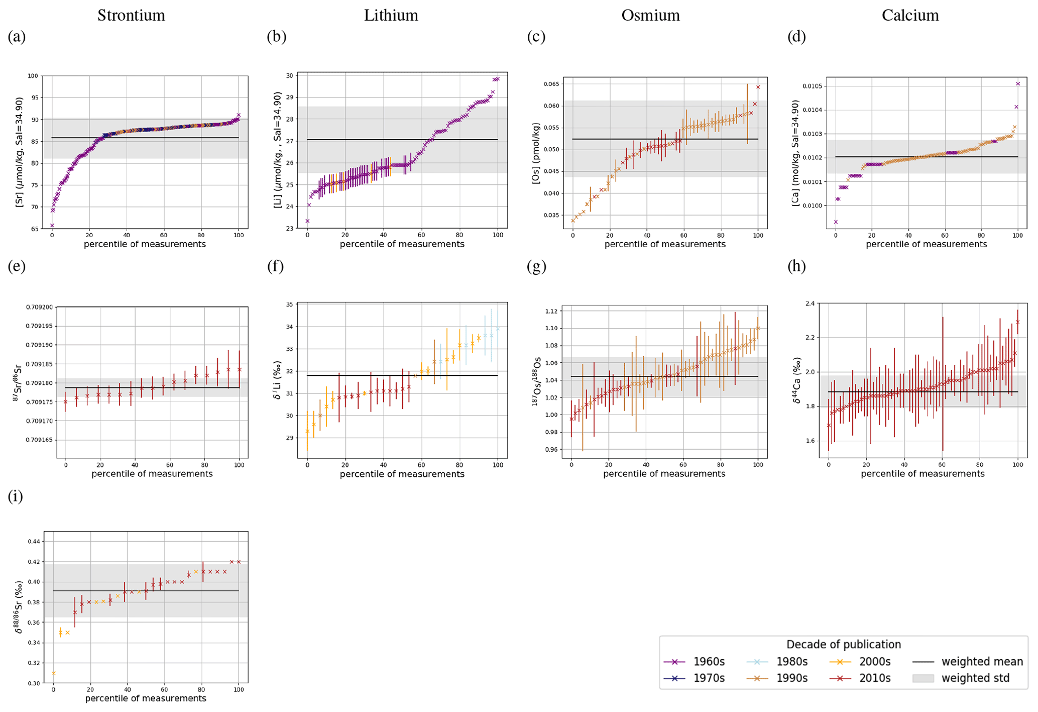
Figure 1Sr (a, e, i), Li (b, f), Os (c, g) and Ca (d, h) composition of modern seawater. Shown are composites of all published measured concentrations (a–d) and isotope ratios (e-i) with reported errors. From these, we calculated mean concentrations and isotope ratios weighted by the reported error (the more uncertain a value, the less it contributes to the mean), which are indicated by horizontal lines. Shading indicates a single weighted standard deviation around the means. Data are taken from Angino et al. (1966), Fabricand et al. (1967), Bernat et al. (1972), Brass and Turekian (1974), De Villiers (1999), Pearce et al. (2015), Mokadem et al. (2015), and the compilation of Wakaki et al. (2017) for Sr; Angino and Billings (1966), Fabricand et al. (1967), Chan (1987), Chan and Edmond (1988), You and Chan (1996), Moriguti and Nakamura (1998), Tomascak et al. (1999), James and Palmer (2000), Košler et al. (2001), Nishio and Nakai (2002), Hall (2002), Bryant et al. (2003), Pistiner and Henderson (2003), Millot et al. (2004), Choi et al. (2010), Pogge von Strandmann et al. (2010), Phan et al. (2016), Lin et al. (2016), Henchiri et al. (2016), Weynell et al. (2017), Fries et al. (2019), Gou et al. (2019), Hindshaw et al. (2019), Murphy et al. (2019), and Pogge von Strandmann et al. (2019b) for Li; Levasseur et al. (1998), Woodhouse et al. (1999) and Gannoun and Burton (2014) for Os; and Fabricand et al. (1967), De Villiers (1999), and Fantle and Tipper (2014) for Ca. The decade of publication is indicated by color as measurement techniques for some metals and isotopes have improved over time. Concentrations of Sr, Li and Ca are normalized to a salinity of 34.90. Os concentrations could not be salinity-normalized because of missing salinity measurements at one out of three measurement sites (Woodhouse et al., 1999).
2.6 Application of Sr, Os, Li and Ca isotopes as proxies of weathering and mantle emissions
The isotopic differences between Sr, Os, Li and Ca in the ocean and exogenic reservoirs make these metals important proxies for mass exchange occurring between the surficial Earth system and the mantle, continental crust (all four) and extra-terrestrial material (Os). Because they record different geochemical pathways, behave differently in water and have different predominant host lithologies, their combined interpretative power is much greater than any one single proxy used in isolation and which is the basis of our model development philosophy here.
Radiogenic Sr and Os isotopes have previously mostly been used separately as proxies for the balance between the weathering of old and juvenile basalt or direct mantle emissions (e.g., Hodell et al., 1990; Goddéris and François, 1995; Tejada et al., 2009; Finlay et al., 2010; Bottini et al., 2012; Dickson et al., 2015). However, in combination, they also provide information about sedimentary rock weathering since continental Sr is primarily derived from carbonates while Os resides predominantly in shales and evaporites (e.g., Peucker-Ehrenbrink et al., 1995). Li is orders of magnitude more abundant in silicates than in carbonates and thus is regarded as the most direct proxy for silicate weathering (Kısakűrek et al., 2005; Millot et al., 2010; Pogge von Strandmann et al., 2020). The isotopic composition of dissolved Li is also not affected by plant growth (Lemarchand et al., 2010; Clergue et al., 2015) or phytoplankton growth (Pogge von Strandmann et al., 2016). Instead, the light Li isotope (6Li) is preferentially taken up by secondary minerals (clays, oxides, zeolites) formed during weathering, enriching residual waters in 7Li. Hence, surface water δ7Li is controlled by the ratio of primary rock dissolution to secondary mineral formation, known as the weathering congruency (Misra and Froelich, 2012; Pogge von Strandmann and Henderson, 2015), which in turn can act as a tracer of weathering intensity (that is, the ratio of the weathering rate to the denudation rate, Dellinger et al., 2015; Pogge von Strandmann et al., 2017; Murphy et al., 2019; Gou et al., 2019). This also relates to the efficiency of CO2 drawdown, as weathering-derived cations cannot assist carbon sequestration in the ocean if they are retained on the continents in secondary minerals (Pogge von Strandmann and Henderson, 2015; Pogge von Strandmann et al., 2017). Ca isotopes have also been used to examine weathering processes in the geological record (Kasemann et al., 2005; Farkaš et al., 2007; Kasemann et al., 2008; Blättler et al., 2011; Holmden et al., 2012; Fantle and Tipper, 2014; Kasemann et al., 2014), and additionally are crucial proxies for the quantification of carbonate precipitation rates (Pogge von Strandmann et al., 2019b), including authigenesis (Fantle and Ridgwell, 2020). Furthermore, Ca isotopes have been considered a potential temperature proxy (e.g., Nägler et al., 2000), but this application might be complicated by the strong control of aqueous chemistry on Ca fractionation (DePaolo, 2011). Alongside Ca, stable Sr isotopes provide information about the dominant form of carbonate burial (Paytan et al., 2021) and growth rate in marine calcifiers, mostly influenced by temperature and pCO2 (Stevenson et al., 2014; Müller et al., 2018). Likewise, changes in the ratio in calcifiers reflect shifts in ecosystem structure, carbonate mineralogy and calcification rate (Stoll and Schrag, 2001).
While each system individually gives valuable insight into Earth system dynamics, in concert these trace metal systems can provide information on feedbacks and event durations, as well as improve the accuracy of our reconstructions (e.g., Kasemann et al., 2008).
For this paper, we developed a series of parameterizations of marine cycling of Sr, Os and Li and Ca isotopes in the Earth system model cGENIE, focusing on the elemental and isotopic fluxes most essential to tracking external metal additions or weathering rate changes. Our implementation is hence deliberately not exhaustive in this initial paper, and representation of elemental cycles, particularly with respect to processes occurring in terrestrial freshwater environments and at the seafloor, could be further improved upon (Sect. 5 discusses ideas for added complexity). The present section provides an overview of the existing implementation.
cGENIE is best described as a modeling framework (Lenton et al., 2007) and comprises, in our study, modules for ocean physics (GOLDSTEIN, Edwards and Marsh, 2005), marine biogeochemistry (BIOGEM, Ridgwell et al., 2007), continental weathering and runoff (ROKGEM, Colbourn et al., 2013), sea-floor sediment formation (SEDGEM, Ridgwell and Hargreaves, 2007), atmospheric chemistry (ATCHEM) and atmospheric energy balance (EMBM, Ridgwell et al., 2007). As such, our implementation of cGENIE includes a 3D ocean combined with a 2D atmosphere and can capture the cycling of carbon and a range of other elements relevant for biogeochemical studies of the ocean water column and at the sea–sediment and sea–air interfaces, as well as climate-sensitive continental runoff and explicit sedimentary carbonate burial.
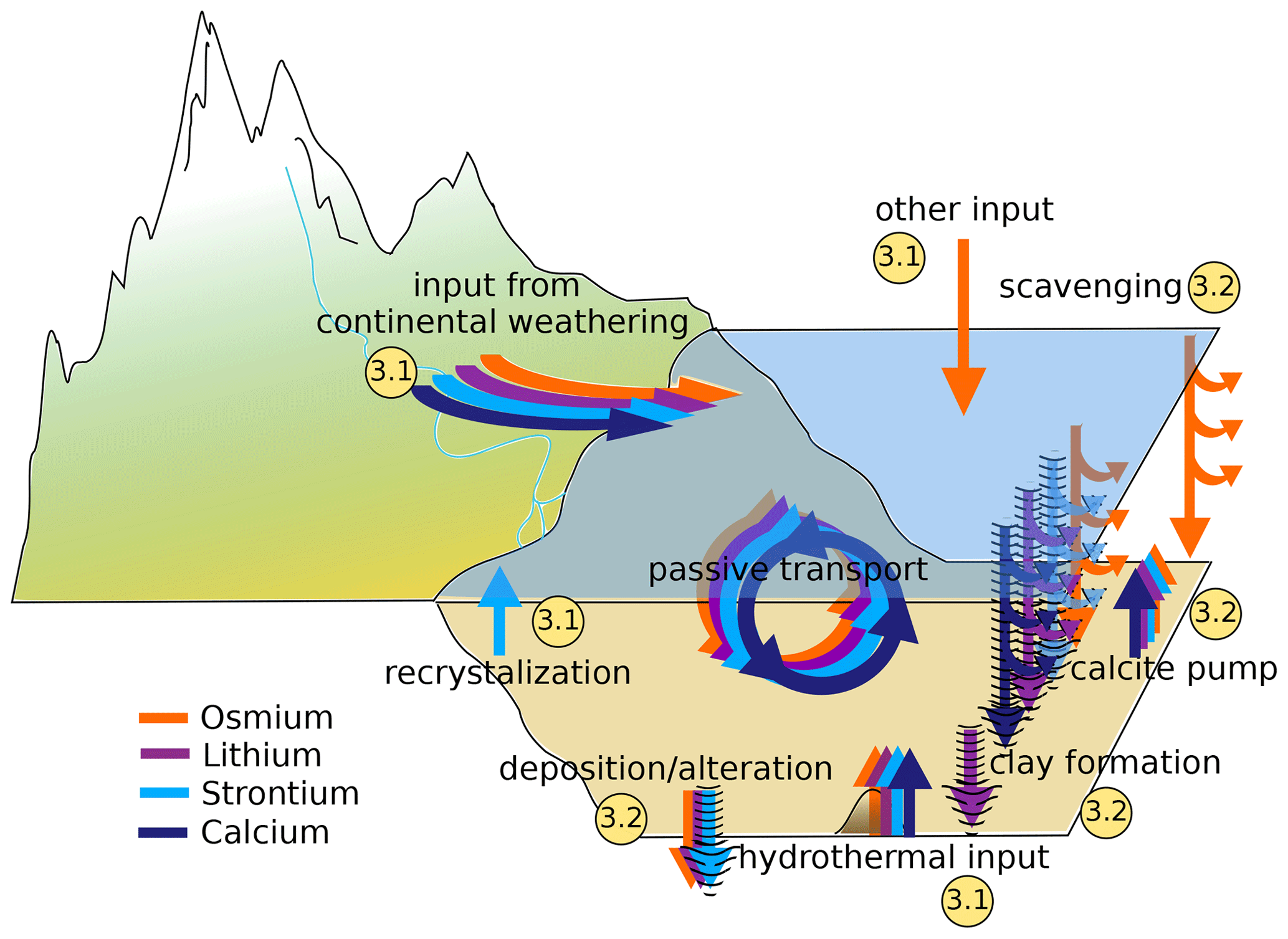
Figure 2Processes included in the cGENIE trace metal implementation and the number of the subsection describing their implementation. Hashed arrows indicate processes during which isotopic fractionation occurs in the model.
Figure 2 shows a conceptual model of the Sr, Os, Li and Ca cycles in cGENIE with arrows of different colors showing mass fluxes of different metals. The implementation of these processes involves code additions to the modules ROKGEM, BIOGEM and SEDGEM that are described in the following sections. Each code addition requires the model user to set parameters controlling the respective metal fluxes. These parameters, as well as a parameter set that reproduces the present-day marine distributions of Sr, Os, Li and Ca in steady-state metal cycles, are provided in Appendix E, together with example experiments as part of the model code release.
3.1 Marine Sr, Os, Li and Ca sources
Continental weathering is the main source for marine Sr, Os, Li and Ca today and changes in the weathered lithology or weathering intensity are invoked as major drivers of the evolution of trace metal concentrations and their isotopic compositions in seawater over time (e.g., Misra and Froelich, 2012; Kristall et al., 2017). ROKGEM, the weathering module of cGENIE, provides a framework for calculating climate- and CO2-dependent additions of Ca, Mg and alkalinity from carbonate weathering (following Berner, 1994) and silicate weathering (following Brady, 1991) to the ocean (see Colbourn et al., 2013, for a full description of the weathering module). By applying linear and exponential relationships of temperature and carbonate and silicate weathering rates, respectively, ROKGEM modifies user-given baseline weathering fluxes according to climatic variations. Additional (optional) modifiers can be selected to represent the effect of changes in precipitation, vegetation and atmospheric CO2 concentration.
The modification of weathering fluxes is either calculated locally, based on a geographic distribution of carbonates and silicates taken from user input (“2-D case”, described in more detail in the Supplement) or globally, based on a globally averaged change in climate (“0-D case”). In both implementations, the ROKGEM module calculates a drainage map based on a prescribed continental topography and determines the coastal locations where weathering input (either of regionally variant composition in the 2D case or homogeneous in the 0D case) is added to the ocean. The flux of metals added to the ocean in these locations is determined by the size of the model catchment and can optionally be scaled by the proportion of global runoff entering the ocean (when rg_opt_weather_runoff=.true.).
Depending on the primary source rock, we tied the rate M of Sr, Os or Li ion delivery to the ocean to Ca and magnesium (Mg) input rates from weathering of carbonates () and/or silicates (), related by a constant ratio k:
ROKGEM allows for different CaSiO3 weathering schemes, including one which separates total CaSiO3 weathering into contributions from granite and basalt weathering. For this case, we imposed individual parameters for Sr weathering for each lithology. Because the amount and isotopic composition of weathering-derived Os is mostly dependent on organic matter content (Jaffe et al., 2002; Georg et al., 2013; Dubin and Peucker-Ehrenbrink, 2015), whereas the 0D weathering scheme in ROKGEM only differentiates between Os delivery from CaSiO3 and CaCO3 weathering. To enable a more realistic simulation of continental Os weathering fluxes, we extended the 2D weathering schemes in ROKGEM to trace Os and its isotopes. While slightly computationally more expensive, Os weathering fluxes can be tied to specific lithologies in these schemes, including organic-rich shales.
The effect of secondary mineral formation on land on Li concentrations and isotope abundances in continental runoff is simulated based on the empirical relationships between the weathering Li flux () and the ratio of weathering to denudation rate (WD, also referred to as weathering congruency) reported in Pogge von Strandmann et al. (2020):
cGENIE derives an estimate of WD from the climate weathering modifier, which adjusts the chemical weathering flux from silicates on the basis of a deviation of climate (e.g., surface land temperature) from some reference value (and a value of WD of 1.0).
To represent the vast range of chemical conditions and reaction rates at the sediment–water interface in the ocean efficiently, three biogeochemically distinct depositional environments are represented in the SEDGEM module: (1) shallow seafloor with reef-building biota (“reef”), (2) shallow seafloor, assumed depleted in oxygen with reef-building biota absent and characterized by organic rich sediments (“muds”), and (3) plankton-derived carbonate (and opal) deposition in the open ocean (“deep sea”). CaCO3 deposition and dissolution, as well as elemental fluxes across the sediment–water interface, are parameterized differently in each of these environments, with masks used to distinguish the different environments.
Mantle-derived metal input via hydrothermal vents is also parameterized in the SEDGEM module and the fluxes to ocean bottom waters occur only in grid cells that represent deep sea. We parameterized this flux such that a global total input flux is prescribed, but it is then either distributed equally across deep-sea grid cells or according to an easily adjustable, spatially explicit map (e.g., following the line of mid-ocean ridges). There is no differentiation between seafloor areas with predominant high- or low-temperature hydrothermal venting in our implementation, and hence we make no isotopic distinction spatially between fluxes from the seafloor. Recrystallization of SrCO3 is an additional source of Sr to the water column (see above). Its parameterization is similar to that for hydrothermal inputs, except that elemental fluxes from recrystallization only occur in bottom waters of grid cells labeled as “reef”. The size and rate of this Sr flux can also either be set as a total global or an area-weighted value.
To account for inputs at the air–sea interface (only assumed to be relevant for Os, as described in the previous section), we added the option to prescribe a spatially explicit field of annual input into the surface ocean (or technically anywhere into the water column).
3.2 Marine Sr, Os, Li and Ca sinks
Ca export from the surface ocean is linked to the export of particulate organic carbon (POC) by a constant CaCO3:POC ratio (rain ratio) (see Ridgwell et al., 2007, for a description of POC export simulation in cGENIE). We parameterize the incorporation of Os, Li and Sr into carbonates by scaling their export in carbonates to the Ca export. This can be done by setting either a constant Sr, Li and Os to Ca ion ratio () or a constant scaling factor α that links the local Sr/Li/Os-to-Ca ratio in seawater to the Sr/Li/Os-to-Ca ratio in the precipitate (following, e.g., Tang et al., 2008):
The Sr/Li/Os-to-Ca ratio of the precipitate is then used to calculate the metal consumption during carbonate formation, as well as metal release during carbonate dissolution. To reflect the different Sr/Li/Os-to-Ca ratios in pelagic compared to reef carbonates, a separate factor can be set for reef production. Reef CaCO3 immediately contributes to surface sediments, whereas pelagically formed CaCO3 sinks through the water column, and might be dissolved before reaching the deep-sea sediment–water interface as a result of local chemical equilibria.
We further included the sequestration of Sr and Li in seafloor sediments due to seafloor weathering by scaling the metal flux into the uppermost sediment layer (fMetal) to the metal concentration of the overlying ocean grid cell ([Metal]):
This burial occurs in all grid cells that are labeled as deep sea. In the absence of better constraints on depositional mechanisms, we include a mathematically similar sink for Os. For a desired global burial rate B (mol s−1), the value of k can be estimated by considering the total area of deep-sea Adeep (m2) and equilibrium metal concentration [Metal] (mol kg−1):
Our model calculates Li burial during clay formation locally at the sea–sediment interface. The burial flux fLiclay is scaled to the concentrations of Li in the deepest grid box of the water column and the detrital flux into the sediments:
To test implications of Os burial with particulate organic carbon, we included an option for [O2]-sensitive scavenging from the water column. In the surface ocean, organic carbon is exported as a function of the concentration of inorganic carbon, light, nutrient availability (PO in our set up), sea ice cover and temperature (Ridgwell et al., 2007). This export production of organic carbon is split into dissolved and particulate organic carbon (DOC and POC) at an adjustable ratio. DOC is advected and diffused in the ocean, while POC is instantly exported to deeper water layers. Remineralization of organic matter can either be set to follow empirical decay functions or to depend on local temperature and redox conditions. Depending on which chemical species are accounted for in a particular experiment, the redox state is calculated based on oxygen, sulfate, methane, nitrate and iron oxide concentrations. O2 is exchanged between the atmosphere and the ocean at the air–sea interface, depending on the solubility of O2 in water. In the ocean, O2 is released during primary production in the surface ocean and consumed during remineralization of DOC and POC under oxic conditions. Sulfur, iron, methane and nitrogen cycling are less relevant for the redox state in the modern open ocean but influenced POC fluxes in the past and are described in detail in van de Velde et al. (2021), Reinhard et al. (2020) and Naafs et al. (2019). Following the example of existing scavenging parameterization schemes in cGENIE, we implemented this by scaling the flux of scavenged Os (fscav) to the local concentrations of Os and POC:
Since there is evidence that Os needs to be reduced in order to be buried, we include a switch to use the scavenging code only where ambient [O2] falls below some specified threshold.
3.3 Isotopes
cGENIE tracks isotopes in total molar abundances rather than delta notation or ratios so that they can be advected and diffused like any other tracer. Li has two stable isotopes, and thus its implementation follows that of other elements with two stable isotopes (e.g., C, Ridgwell, 2001; Ridgwell et al., 2007). The addition of Sr, Os and Ca isotopes needed different approaches because they have more than two principal stable isotopes. We chose to reduce the number of traced isotopes to three for Sr and Os and to two for Ca because these subsets contain the most abundant isotopes of the respective element (Sr) and/or are most relevant for their application as seawater proxies (Sr, Os and Ca). Calcium is thus currently treated like an element with two stable isotopes in cGENIE. To track three isotopes rather than two, we track two isotopes explicitly and one implicitly by subtracting from the bulk abundance of the trace metal. In the case of Sr, abundances of 87Sr and 88Sr are tracked explicitly. The abundance of 86Sr is then taken as the difference between the abundances of the two explicitly tracked isotopes and the bulk Sr abundance, since 84Sr can be neglected. Os has more than two stable isotopes, but only two of them, 187Os and 188Os, are currently used as a proxy system, and thus these two isotopes are tracked explicitly and the bulk Os abundance contains all remaining stable isotopes.
Every metal flux in the model is accompanied by fluxes of the traced isotopes. The scale of these isotope fluxes depends on the size of the metal flux and the relative abundance of the respective isotope, derived from the model configuration in which the model user prescribes the isotopic composition of marine metal inputs and outputs. For simplicity, the user can prescribe these isotopic compositions in delta notation for stable isotopes and ratios for radiogenic isotopes. The model then converts these values into molar isotope abundances, using the isotope standards listed in Table 5 (international standards where available and observations of modern-day seawater otherwise). If required, these internal standards can be changed by the user, although this currently requires an edit to the code.
Mokadem et al. (2015)Nier (1938)Lu et al. (2017)Dąbek and Halas (2007)Heuser et al. (2002)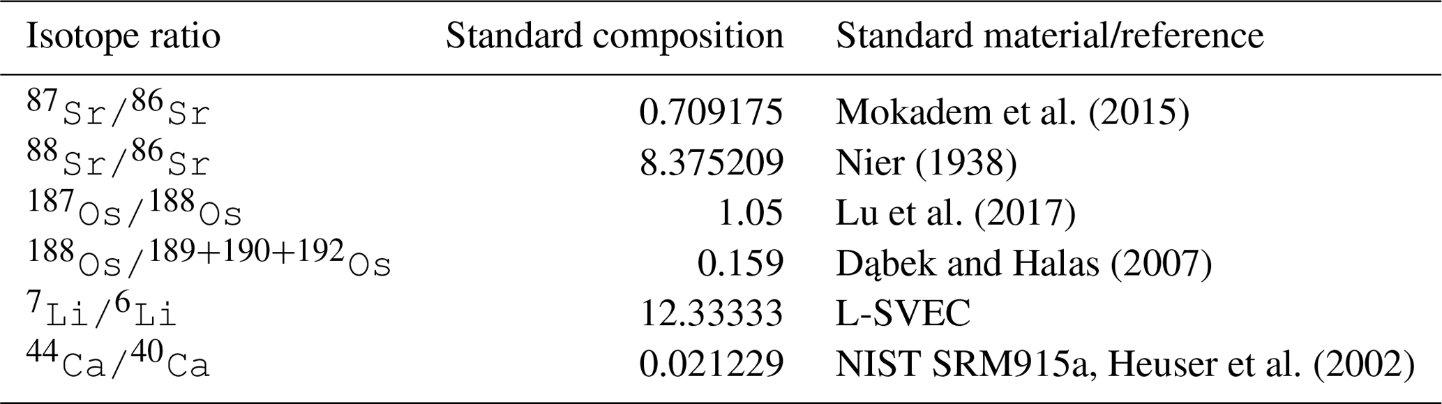
Given the current lack of evidence for Os isotopic fractionation outside of the lithosphere (e.g. Nanne et al., 2017), we do not include a fractionation factor for marine Os sinks (or rather, it is assume to be 1.0). For Sr and Li, we account for isotopic fractionation during carbonate and secondary mineral formation. In its default setting, cGENIE uses constant fractionation factors for Sr, Li and Ca fluxes, but we have included optional schemes to simulate environmental controls on stable Li and Ca isotope fractionation. For Li, we included an optional correction of riverine δ7Li for weathering congruency (following Pogge von Strandmann et al., 2020) and the temperature sensitivity of Li isotope fractionation during terrestrial and marine clay formation (Millot et al., 2010):
with being the assumed δ7Li of weathered silicates at the reference temperature, k the isotopic effect of a 1 ∘C temperature change and T0 being the reference temperature. A consistency check prevents the resulting δ7Lirunoff from falling below the composition of continental crust. If these functions are not used, the absence of simulated Li fractionation in freshwater should be taken into account by setting the parameters for terrestrial Li input based on the composition of river water rather than weathered Li at the reference temperature.
cGENIE also offers two different choices for Ca isotope fractionation during carbonate formation (in addition to the default of a fixed fractionation), carbonate ion concentration-dependent fractionation following Gussone et al. (2005) and saturation state (Ω)-dependent fractionation following Tang et al. (2008):
These fractionation schemes are explored in Appendix C, as well as in Fantle et al. (2020).
The model parameters required to set isotopic fractionation of Os, Li and Sr are listed in Table E8.
The three-dimensional grid of cGENIE allows for comparison of the spatial pattern produced by the simulated set of processes to observations, which can further bolster or challenge our assumptions about global trace metal cycling on diverse timescales. Here we set up the model to represent the pre-industrial state of trace metal cycling, and compare the model output to measured modern seawater profiles.
4.1 Pre-industrial configuration
We initialized cGENIE with a modern-day geography on a 36×36 grid with eight depth layers in the ocean (following Ridgwell and Hargreaves, 2007) and with a pre-industrial CO2 concentration of 278 ppm. Marine biological productivity is simulated using a single-nutrient scheme as outlined in Ridgwell et al. (2007), but here it is done with a constant CaCO3:POC rain ratio set to 0.043, in line with typical paleo-configurations of the model (Panchuk et al., 2008). Burial and dissolution of CaCO3 in deep-sea sediments follows Ridgwell and Hargreaves (2007). This configuration results in a pelagic CaCO3 burial rate of 0.125 PgC yr−1, close to the observationally calibrated CaCO3 sink of Ridgwell and Hargreaves (2007). In addition to the pelagic environment, covering 350.6 million square kilometers, we simulated reef deposition on shelves, which covers 5.5 million square kilometers in our particular (low-resolution) modern model grid (see Appendix D). The sediment model bathymetry was derived from ETOPO5, Data Announcement 88-MGG-02, 1988). Reefal deposition was simulated in grid cells representing marine sediments shallower than 1000 m and not further polewards than 41.8∘ N/S, on the basis that reefal carbonate deposition is predominantly a tropical and subtropical process. We prescribe a reefal CaCO3 sink of 0.05 PgC yr−1 associated with these environments (approximately 40 % of the deep-sea value). Temperature-dependent terrestrial silicate and carbonate weathering (Lord et al., 2016) formulations were selected, with the baseline temperature and rates of carbonate and silicate weathering set to 8.48 ∘C, 8.4 and 6.0 Tmol yr−1, respectively. Silicate weathering was split into the CO2-consuming weathering components: CaSiO3 () and MgSiO3 (). In the absence of a numerical representation of hydrothermal cation exchange (Coogan and Gillis, 2018), we balanced the Ca and Mg cycles by including a constant exchange between sedimentary Ca and dissolved Mg of 2.0 Tmol yr−1 at the seafloor. To close the long-term carbon cycle, we prescribed a fixed rate of organic C burial of 0.031 PgC yr−1 with ‰, as well as a total exogenic carbon influx of 0.103 PgC yr−1 with ‰. This net input can be regarded as the result of 0.103 PgC yr−1 subaerial outgassing with ‰ (Mason et al., 2017), hydrothermal emissions of 0.018 PgC yr−1 with ‰ at mid-ocean ridges and consumption of 0.018 PgC yr−1 with δ13C=2 ‰ during seafloor weathering (Cocker et al., 1982).
Table 6 summarizes the trace metal fluxes we prescribed to simulate the pre-industrial trace metal cycling, consistent with the observational constraints provided in Tables 1–4. We used the 0D weathering scheme for computational efficiency, but since a differentiation between carbonate and silicate derived Os does not capture the lithology dependence of the Os weathering flux appropriately, we prescribed the net abundance and isotopic composition of Os in continental runoff rather than lithology-specific compositions. We also did not simulate Os scavenging in these pre-industrial spin-ups because the dependence of marine Os burial on organic matter abundance and redox state are uncertain and today's ocean is predominantly oxic. However, in Appendix A1 and A2 we included the results of two pre-industrial Os cycle spin-ups – one with the 2D weathering scheme and the second with Os scavenging under occurring anoxic conditions and accounting for 50 % of marine Os burial. Note that the prescribed hydrothermal metal fluxes are net fluxes of high- and low-temperature hydrothermal activity. The specific model parameters that need to be prescribed to achieve these fluxes are given in the Supplement and in the GitHub repository containing all relevant configuration files, which can be accessed as outlined under “code availability”.
In running the model to steady state, we assume that metal fluxes are currently in equilibrium. This is a common assumption when modeling weathering tracer isotopes and their perturbations in the geological record (e.g., Misra and Froelich, 2012; Bauer et al., 2017). However, given the long residence time estimates in today's ocean, it is likely that at least the Sr, Li and Ca cycles are not fully in steady state today (i.e., Derry, 2009). For example, Paytan et al. (2021) inferred that the marine Sr has constantly fluctuated over the last 35 Myr. Constant Os isotopic compositions of seawater over the last millennia suggest that Os has reached steady state since the last deglaciation. However, residence time estimates of >20 kyr based on modern day Os fluxes put this into question (Oxburgh, 2001). The newly implemented tracers in cGENIE can be used to study different equilibria and transient adaptations of the marine metal reservoirs to new boundary conditions. For example, we were not able to simulate the observed marine Sr reservoir using the observed Sr input fluxes, which indicates an imbalance between observed Sr fluxes and the marine Sr reservoir. Hence, we simulated two different steady states for Sr under pre-industrial boundary conditions: one with a best estimate of pre-industrial Sr fluxes (hereafter referred to as FLUXES) and one tuned to best fit the spatial mean of observations (TUNED).

The model spin-up was carried out in three stages to improve computational efficiency. The first stage (20 kyr) was carried out with a “closed” marine carbonate system, where the marine C and alkalinity reservoirs are artificially restored by balancing losses through CaCO3 burial with external inputs to the ocean. During this stage, the climate and ocean dynamics adjust to the physical boundary conditions and ocean–atmosphere C exchanges come into balance. In the second phase (500 kyr), the marine carbonate system was “open” so that prescribed inputs from terrestrial weathering and the mantle and marine burial dynamically adjusted to balance one another. During the third stage (15 Myr), when ocean dynamics, C, nutrient and Ca cycles were already equilibrated, the prescribed Sr, Os and Li sources were added, and the model was run until metal concentrations and their isotopic composition in the ocean were at steady state. The model calculations were accelerated during the last two stages of the spin-up using the time-stepping method introduced by Lord et al. (2016).
4.2 Comparison between simulated and observed trace metal contents of seawater
One advantage of simulating trace metal cycles within a 3D Earth system model is that we can test simulated metal concentrations and isotopes against observed spatial patterns. In the following sections, the simulated pre-industrial distribution of each metal is compared against observational data shown in Sect. 2.5.
4.2.1 Strontium
Figure 3 compares Sr concentrations and isotopic compositions in our simulation with observations. The simulated marine Sr reservoir is more homogeneous than observed in terms of concentrations and isotopic composition. The FLUXES simulation, in which we prescribe observationally constrained marine Sr inputs, results in more radiogenic and isotopically heavy marine Sr than observed. To yield a steady-state marine close to observations, we need to assume that the continental Sr supply is on average less radiogenic than observed (in agreement with, e.g., Pearce et al., 2015). Similarly, the observed fractionation factor for stable Sr isotopes during biogenic CaCO3 formation is too large to equilibrate the model at the observed low Sr if we do not assume that all Sr sources only provide mantle-like light Sr ( ‰, TUNED simulation). Corroborating the conclusion of, e.g., Vance et al. (2009), this suggests that the isotopic composition of marine dissolved Sr is currently not at equilibrium.
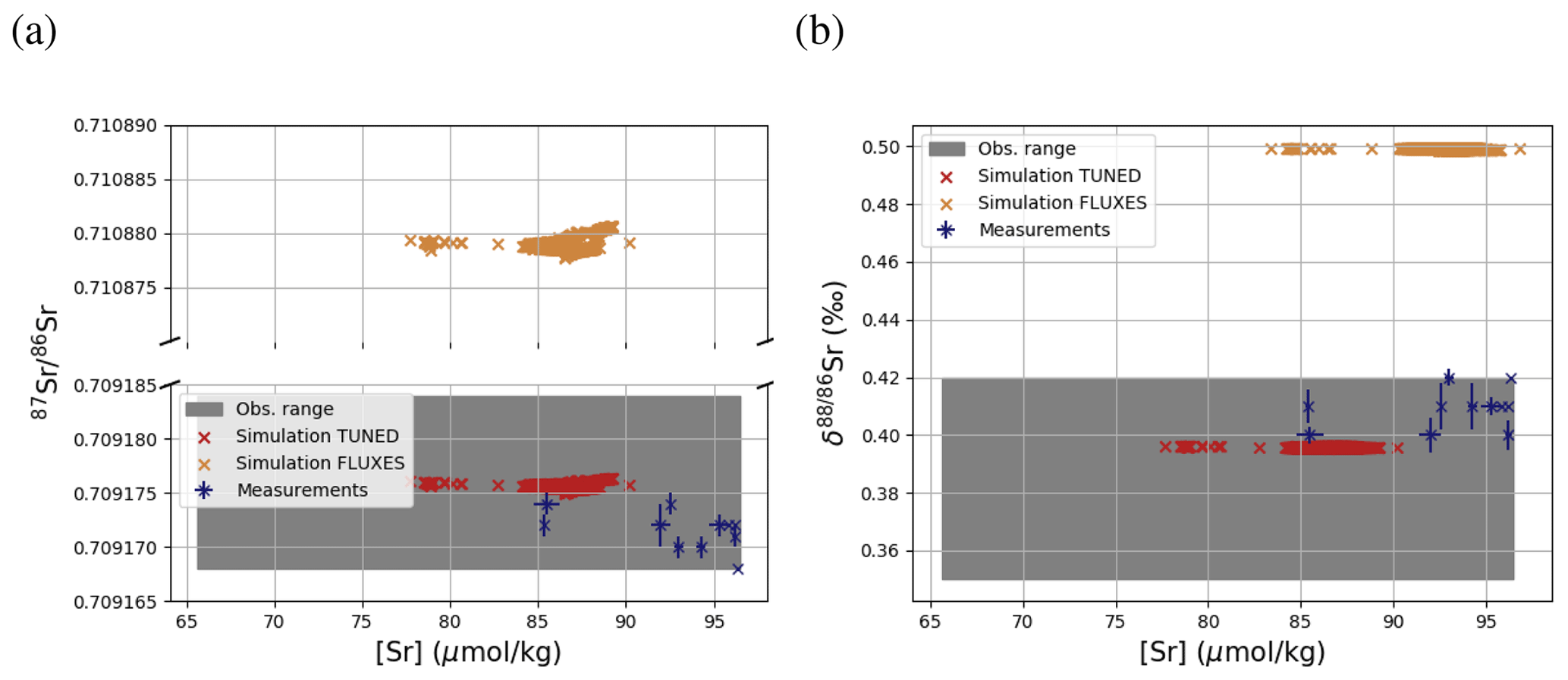
Figure 3Comparison between measured and simulated concentrations (a) and isotopic composition (b) of dissolved Sr in seawater. The displayed data points are paired measurements of Sr concentrations and isotope ratios (Wakaki et al., 2017), while the gray box also indicates the full range of concentrations and isotopic compositions (separate measurements of Sr concentration or isotope ratios) (Angino et al., 1966; Fabricand et al., 1967; Bernat et al., 1972; Brass and Turekian, 1974; De Villiers, 1999; Mokadem et al., 2015). Observations and model results are salinity-normalized.
The simulations capture the homogeneous vertical profiles of Sr concentrations observed at most sites (see Figs. F1 and F5). One exception are modeled Sr concentrations in the North Atlantic, which are high compared with older measurements. Given that these low observed North Atlantic values come from one of the first studies measuring Sr concentrations in seawater (Angino et al., 1966) and that other studies of North Atlantic seawater yielded higher Sr concentrations (e.g., De Villiers, 1999), this difference could be partially the result of analytical errors, although influences from seasonal or inter-annual variability not captured by the model cannot be ruled out.
4.2.2 Osmium
Os concentrations and isotopes are generally more spatially homogeneous in the simulation compared with observations. For 80 % of the paired measurements of Os concentrations and isotopic compositions, one or more cGENIE simulated grid cells fall within measurement uncertainty. The remaining 20 % of the Os observational data (those measurements with the lowest Os concentrations and isotopic ratios) were not reproduced in any grid cells in our simulation. This discrepancy between model simulation and observations is not the result of the simplified homogeneous terrestrial Os input in the model. In a repetition of the model experiment but employing spatially variable Os input (see Fig. A1), we found no appreciable change to the simulated ranges of Os concentrations and isotope ratios in the oceans, i.e., no appreciable increase in spatial heterogeneity. Since the low Os concentrations not captured by the model are observations from surface and intermediate waters from the East Pacific (Fig. F6, Woodhouse et al., 1999; Gannoun and Burton, 2014), some processes affecting Os removal in that region might instead be missing in our model. For example, Woodhouse et al. (1999) suggested that Os could bind onto organic matter in the water column under low-oxygen conditions.

Figure 4Comparison between measured and simulated concentrations and isotopic composition of dissolved Os in seawater. Shown are all available measured Os concentrations and isotope ratios for the modern ocean alongside the values of all ocean grid cells in the simulation. Data are taken from Levasseur et al. (1998), Woodhouse et al. (1999), and Gannoun and Burton (2014).
We tested the effect of increased Os removal with particulate organic matter from anoxic water masses in cGENIE by associating half of the marine Os burial with the optional Os scavenging sink (Eq. 9, see the results of our sensitivity study in Sect. A2). The true magnitude of Os burial associated with organic matter is uncertain, but we assumed here that it is responsible for all suboxic Os removal, which is estimated to account for at least 50 % of total marine burial flux that we assumed (Lu et al., 2017). Adding such dependence of Os burial on environmental conditions increased the range of simulated Os concentrations beyond that observed; i.e., Os scavenging is more than capable of producing the observed spatial heterogeneity in Os concentrations. However, there is no known Os isotopic fractionation associated with scavenging or burial; in the absence such fractionation, scavenging does not increase the range of simulated marine Os isotope ratios. Observations from sites outside the East Pacific show no vertical Os concentration gradients, which is well reproduced by our simulation set-up. The Os isotopic composition shows a uniform vertical distribution in the simulations, which is consistent with observations at all sites (see Fig. F6). While our initial simulation is thus consistent with the majority of Os measurements, we showed that cGENIE provides the necessary framework to investigate regionally variable environmental controls on the marine Os reservoir.
4.2.3 Lithium
Similar to Sr and Os, the model simulations fall within the range of observed concentrations and isotopic compositions of dissolved Li, although they are more homogeneous than observed (see Fig. 5). cGENIE can be used to explore whether environmental influences on local Li inputs and burial can explain this disparity, though underestimated measurement uncertainties and inter-laboratory inconsistencies, particularly in older studies, could also contribute to the spread in observed values. For example, the high concentrations, which are underrepresented in our simulation (see Figs. F7 and F3), come from one study in the Caribbean Sea (Angino and Billings, 1966), a marginal ocean that is not representative of the open ocean and which might not be sufficiently resolved in the coarse grid of cGENIE. However, Angino and Billings (1966) was one of the first studies measuring Li concentrations in seawater, and their measurements may be associated with much larger uncertainties than reported. Were these measurements excluded, the spatial mean of observed Li concentrations would be lower, and the model could be retuned by prescribing slightly lower Li fluxes in and out of the ocean, which would be permissible given the current range of flux estimates (see Table 3).

Figure 5Comparison between measured and simulated concentrations and isotopic composition of dissolved Li in seawater. The displayed data points are measurements of Sr concentrations and isotope ratios on the same samples (Hall, 2002), while the gray box also indicates the range of concentrations and isotopic compositions that were measured separately (Angino and Billings, 1966; Fabricand et al., 1967; Chan, 1987; Chan and Edmond, 1988; You and Chan, 1996; Moriguti and Nakamura, 1998; Tomascak et al., 1999; James and Palmer, 2000; Košler et al., 2001; Nishio and Nakai, 2002; Bryant et al., 2003; Pistiner and Henderson, 2003; Millot et al., 2004; Choi et al., 2010; Pogge von Strandmann et al., 2010; Lin et al., 2016; Henchiri et al., 2016; Phan et al., 2016; Weynell et al., 2017; Fries et al., 2019; Gou et al., 2019; Hindshaw et al., 2019; Murphy et al., 2019; Pogge von Strandmann et al., 2019b). Observations and model results are salinity-normalized.
Only one measured vertical profile of Li isotopes is available in the literature (Hall, 2002), and it shows no vertical δ7Li variation, which is reproduced by our simulation. The simulated 7Li is offset from the profile reported by Hall (2002) since we tuned the model to the average of reported seawater 7Li measurements but the profile in Hall (2002) contains some of the most 7Li-enriched published seawater values.
4.2.4 Calcium
Simulated concentrations of dissolved Ca and its homogeneous isotopic composition closely resemble the observations, the spread in observed Ca isotope ratios likely being due to measurement uncertainty given the large reported error bars (see Fig. 1). Repeating our model spin-up with different parameterizations of Ca isotope fractionation during biogenic carbonate formation did not appreciably increase the simulated range of marine Ca isotope ratios (see our sensitivity study in Sect. C). Similar to the average Ca concentration in seawater, the uniform vertical distribution is well captured by the model simulation (see Fig. F8). Likewise, no vertical gradients are observed or simulated. Observed ratios are in between simulation results with tuned and untuned marine Sr reservoirs. This is an artifact of the tuning to mean observed Sr concentrations, which is lower than the mean Sr concentrations of the sites shown in Fig. F8 because it includes the anomalously depleted samples from the North Atlantic. This mismatch is another indication that the Sr measurements reported in Angino et al. (1966) might be associated with a larger uncertainty than reported.
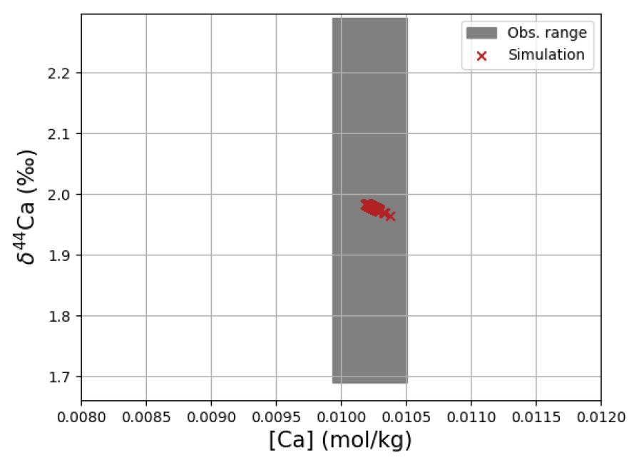
Figure 6Comparison between measured and simulated concentrations and isotopic composition of dissolved Ca in seawater. The gray box indicates the range of concentrations and isotopic compositions that were measured on separate samples (Fabricand et al., 1967; De Villiers, 1999; Fantle and Tipper, 2014). Observations and model results are salinity-normalized.
4.3 Transient perturbation experiments
Adding the new metal cycles to cGENIE now enables us to study their transient behavior under external forcings in a fully coupled system, including effects from ocean circulation and primary productivity changes, climate-sensitive weathering, and marine carbonate accumulation and dissolution. Here we present one such example, where we instantaneously release either 1000 or 5000 Pg C into the atmosphere to produce temporary weathering responses which gradually re-equilibrate the model (similar to Lord et al., 2016). These scenarios allow us to showcase the sensitivity of the simulated metal systems and to discuss the Earth system processes that shape their transient evolution. Our experiments are set up to understand model behavior rather than to compare against any particular geological records or represent any particular event, although the choices of carbon release relate to estimates associated with differing “hyperthermal” events of the Paleogene (e.g., Panchuk et al., 2008; Kirtland Turner and Ridgwell, 2013). It is also important to note that some of these scenarios generate isotopic perturbations smaller than the analytical uncertainty of real-world measurements.
Table 7Marine trace metal concentrations and residence times in our pre-industrial spin-up compared to those reported in literature (see scientific background).

In our spin-up, the prescribed metal fluxes result in residence times within the range of published estimates (Table 7). Li has the longest residence time in our simulations, and thus the largest inertia to external perturbations. Sr and Ca follow, with Os being the most responsive system.

Figure 7Transient changes in modeled Sr, Os, Li, Ca, composition of seawater, and atmospheric CO2 and temperature following instant releases of 1000 and 5000 Pg C. Shown are changes (a) in concentrations, and (b) in the isotopic composition of seawater.
Figure 7 shows the modeled transient response of Sr, Os, Li, Ca concentrations and isotopic compositions to an exogenic CO2 pulse, together with mean global ocean dissolved inorganic carbon (DIC) δ13C, atmospheric CO2 and temperature. After the instantaneous carbon release, atmospheric CO2 concentration increases and the δ13C of seawater decreases on the timescale of years. The increase in atmospheric CO2 and invasion of CO2 into the ocean also suppresses biogenic carbonate formation in the surface ocean and leads to the dissolution of pelagic carbonates. Over the next ∼10 000 years, “carbonate compensation” removes the majority of the initial excess carbon from the atmosphere (Lord et al., 2016). Increased atmospheric CO2 also enhances the greenhouse effect and thus leads to a rise in global mean air temperature, altering the hydrological cycle and speeding up reaction kinetics, in turn resulting in increased rates of continental crust weathering. After a few tens of thousands of years, increased continental weathering supplies enough alkalinity to the ocean to reverse the dissolution of carbonates on the seafloor and increase carbonate burial. Through enhanced silicate weathering and carbonate burial, the remaining excess carbon is sequestered over the timescale of ∼100 000 years after the initial emissions pulse. Over the same timescale, temperature, which due to Earth system feedbacks initially recovers more slowly than atmospheric CO2 concentrations, returns to pre-emissions values and ends the phase of enhanced weathering.
Metal input from continental weathering (and marine carbonate dissolution for Sr and Ca) leads to a transient growth of marine metal reservoirs and isotopic excursions. Increased continental weathering increases the influx of radiogenic Sr and Os, driving the respective marine reservoirs to more radiogenic isotopic compositions. The continental crust is also depleted in heavy stable isotopes compared to seawater, such that the increased weathering influx reduces the Sr, δ7Li and δ44Ca values of seawater. The isotopic composition of carbonates and silicates in continental crust is spatially uniform in our set-up, and cGENIE does not simulate any isotopic effects associated with changes in erosion rate. By default, isotopic shifts due to changes in secondary mineral formation and dissolution in freshwater systems are also not simulated. However, such a shift has been deduced from observed δ7Li isotope excursions (e.g., for δ7Li, Lechler et al., 2015). Enabling the climate-sensitive parameterization of δ7Li in continental runoff demonstrates that this can increase the excursion amplitude to be more consistent with perturbations in the geologic record (see our sensitivity study in Sect. B).
At steady state, alkalinity and Ca2+ inputs to the ocean are equal. Since the alkalinity supply is entirely derived from climate-sensitive continental weathering but one-third of the Ca2+ influx is derived from a constant hydrothermal source, the climate-driven increase in weathering results in a temporarily larger supply of alkalinity than of Ca2+, which does not occur in C-cycle simulations without an igneous Ca2+ source at the seafloor (e.g., Lord et al., 2016; Vervoort et al., 2019). The imbalance between alkalinity and Ca2+ input is small (10 % of the Ca2+ input at its peak), but cumulatively enough excess alkalinity is supplied to cause a slight reduction of the steady-state marine Ca and Sr reservoirs (by ∼0.5 % following the emission of 5000 Pg C). Our assumption of a climate-insensitive Ca2+ source at the seafloor is a simplification since there is evidence that this flux varies with bottom-water properties, in particular temperature (e.g., Krissansen-Totton and Catling, 2017). However, the temperature sensitivity of the seafloor Ca2+ influx is likely lower than that of continental weathering (Brady and Gíslason, 1997), and temperature change is dampened in the deep ocean. Thus, even if the temperature sensitivity of hydrothermal Ca2+ input was considered, a temporary imbalance of alkalinity and Ca2+ supplies during a transient warming event is likely when alkalinity and Ca2+ enter the ocean via different pathways. Our set-up thus produces an upper limit for such a transient imbalance between alkalinity and Ca2+ supply, assuming constant seafloor fluxes.
In the presented simulations, only the excursion amplitudes of radiogenic and δ7Li assuming climate-driven runoff modifications are larger than measurement uncertainty in present-day seawater (see Figs. 3–6). Stronger or prolonged climate change, a larger isotopic offset between seawater and continental runoff, or a more sensitive weathering regime would be required to produce detectable weathering changes in the other isotope systems. Regardless, our idealized perturbation of the modern system illustrates the differing responses of all five isotope systems to a C emission pulse. Specifically, we find that the timings of excursion peaks and minima differ strongly between the isotope systems, which might provide a “fingerprint” of rapid C injection. For instance, the radiogenic and negative Sr and δ44Ca excursions peak a few tens of thousands of years after the C injection, while the radiogenic and negative δ7Li excursions take hundreds of thousands of years to reach their full amplitude. These time lags result from different residence times and fractionation processes.
With the shortest residence time, estimated both from present-day inventories and in our simulation (see Table 7), Os is the first metal to re-equilibrate after the perturbation. The excursions in Os concentration and isotopes are only driven by enhanced weathering rates, and thus both recover within 300 kyr once atmospheric temperature, and with it continental weathering rates, decrease sufficiently. The radiogenic excursion, however, continues to grow until weathering rates have fully returned to pre-event levels because concentration-dependent Sr sinks adapt more slowly to enhanced continental Sr input as a result of the longer residence time. The re-equilibration of the marine Sr reservoir is substantially slower than that of the Os reservoir for the same reason. However, the removal of marine Sr is also dependent on carbonate chemistry, since marine carbonate preservation constitutes the largest marine Sr sink. Biogenic carbonate preservation initially decreases because of the pH and carbonate saturation drop following the C injection, but it increases during the C cycle recovery as a result of enhanced weathering-related alkalinity input. Increased marine carbonate burial causes the marine Ca reservoir to re-equilibrate on a similar timescale to Os, although Ca has a substantially longer residence time in our spin-up. The effect is not strong enough to stop the growth of the marine Sr reservoir, but it reduces its growth rate. Isotopic fractionation of Ca and Sr during biogenic carbonate formation enhances the speed of the δ44Ca recovery and stops the Sr excursion from growing, despite continued excess input of isotopically light continental Sr. Li has the longest residence time of the four metals in our simulations, and Li burial is only dependent on the marine Li concentration and not carbonate chemistry. Hence, the marine Li reservoir continues to grow until all excess weathering stops. Once more dissolved Li is buried than added to the ocean, i.e., the marine Li reservoir shrinks, the δ7Li trend reverses because excess sources of isotopically light Li cease and isotopically light Li is preferentially buried during clay formation, enriching seawater in the heavier 7Li. In the longer term, stable isotope fractionation during the removal of excess Sr, Li and Ca from the ocean results in transient positive Sr, δ7Li and δ44Ca excursions which, in the case of Sr and Li, last for several million years. In our simulations, the staggered timings of the and excursion peaks, as well as the δ44Ca and δ7Li excursion minima, are thus predominantly the result of different elemental residence times, while enhanced carbonate burial is the main reason for the time lag between δ7Li and Sr and the coincidence of the excursion minima of Sr and δ44Ca.
Incorporation of Sr, Os, Li and Ca cycle dynamics in cGENIE constitutes a useful tool to study perturbations of marine metal reservoirs during environmental changes and, importantly, in concert with other biogeochemical tracers. Several extensions of this model can be envisaged to include the representation of metal-specific processes that we did not address in this initial cGENIE implementation. Firstly, the SEDGEM module could be expanded by adding temperature dependency to the fluxes of Sr, Os, Li, Ca, C and Mg related to seafloor alteration. Although secular variation in Cenozoic climate altered these fluxes by an order of magnitude less than those connected to terrestrial weathering (Krissansen-Totton and Catling, 2017), this extra model feature could still improve the simulated metal isotope response to long-term environmental change and constrain metal fluxes in warmer Earth system states. Secondly, the weathering module ROKGEM could be extended to simulate C and S release from organic shale weathering alongside Os fluxes to better capture the climatic and biogeochemical effects of changing shale weathering. Thirdly, celestite-bound Sr could be added as an additional particulate Sr tracer to improve the representation of Sr cycling in oceans with higher celestite stability than at present. Similarly, growth rate-dependent isotope fractionation factors could be implemented in the ecosystem module ECOGEM (Ward et al., 2018). However, the benefit of more complex biological metal cycles will have to be weighed against increased computational costs and the need to constrain additional rate constants and fractionation factors.
Sr, Os, Li and Ca isotope records can help identify mantle activity and lithological responses to climate change in the geological record if processes governing their distribution in the ocean and their response to geological perturbations are well understood. Our implementation of the marine cycling of Sr, Os, Li and Ca in the Earth system model cGENIE allows us to investigate these processes and their consistency with observations. Simulating pre-industrial Sr, Os, Li and Ca distributions in the ocean, the model achieves slightly more homogeneous fields than observed but is consistent with the widely used assumption of homogeneous metal isotope distributions in a fully equilibrated state (e.g., Elderfield, 1986; Chan and Edmond, 1988). It reproduces the mostly homogeneous mean observed depth profiles of concentrations and isotopic compositions well but partially deviates from local observations. This could be an artifact of measurement uncertainties, non-equilibrated cycles in today's ocean, or local processes that are not resolved or parameterized in cGENIE. We showed how this new cGENIE tracer development provides an opportunity to investigate the consistency between reported metal compositions in the ocean and marine sources and sinks. Further investigations of the differences between cGENIE simulations and observations thus have the potential to improve our understanding of present-day marine trace metal cycling. Furthermore, the new implementation can be used to study the response of these metal cycles to transient environmental change. As an example, we showed how these systems respond to a sudden CO2 release through perturbation to their input and output fluxes on different timescales. cGENIE thus becomes a valuable tool to quantitatively interrogate the environmental signals of these isotope systems as preserved in sedimentary records and their relationship to more traditional isotope systems such as carbon.
We tested two additional Os cycle set-ups besides the pre-industrial spin-up described in the main paper: one with a 2D continental weathering scheme in which Os delivery is tied to organic-rich shale and basalt weathering, and one assuming that half of marine Os deposition happens through association with POC in anoxic conditions. The following two subsections show the two set-ups and the simulation results.
A1 Continental Os inputs calculated with a 2D weathering scheme
We added Os and stable isotope (187Os and 188Os) tracers to the 2D weathering schemes available in ROKGEM (Colbourn et al., 2013). Derived from Suchet and Probst (1995), Bluth and Kump (1994), Gibbs and Kump (1994), and Gibbs et al. (1999), these weathering schemes calculate alkalinity and DIC fluxes entering coastal grid cells based on lithology-specific dependencies on runoff. Depending on the scheme, the model user can specify the locations of five or six pre-defined lithologies (carbonates, sandstone, shales, basalt, granites), the relative contribution of weathering fluxes from these lithologies to the overall input of carbonate- and silicate-derived weathering fluxes to the ocean, and parameters that define the sensitivity of these fluxes to runoff changes. Similarly, flux and isotopic composition of Os derived from each of these lithologies can now be prescribed by changing the input files of ROKGEM (see the cGENIE.muffin manual, p. 372–373, for a step-by-step guide). To test the effect of spatially explicit Os weathering fluxes on the isotopic composition of dissolved Os in the ocean, we tied the continental Os weathering flux to shale and basalt weathering, which are assumed to be dominant continental Os sources (Li et al., 2009). We ascribed typical isotopic compositions ( for shales, Dubin and Peucker-Ehrenbrink, 2015, and for basalt, Peucker-Ehrenbrink and Jahn, 2001) to Os derived from these lithologies and Os yields that resulted in the same global Os weathering input as in the pre-industrial spin-up presented in the main text (2605 mol Os yr−1 with ).
Table A1Model parameters setting Os scavenging under sub-oxic conditions.
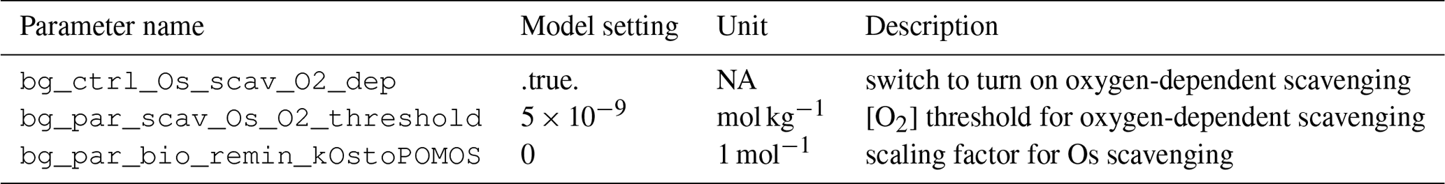
Figure A1 shows the simulated spatial pattern of Os weathering flux alongside measurements. The comparison between Os concentrations in rivers and in cGENIE runoff is complicated by the high reactivity of Os in river deltas (Turekian et al., 2007), which might result in lower Os addition to the open than to the coastal ocean. However, there is general agreement between the measured and simulated isotopic composition of local Os weathering fluxes. This spatially heterogeneous Os weathering flux does not change the ranges of simulated marine Os concentrations and isotope ratios substantially (Fig. A2), suggesting that assumptions about the homogeneity of marine Os inputs are not the cause of differences between the simulated and observed marine Os reservoir.
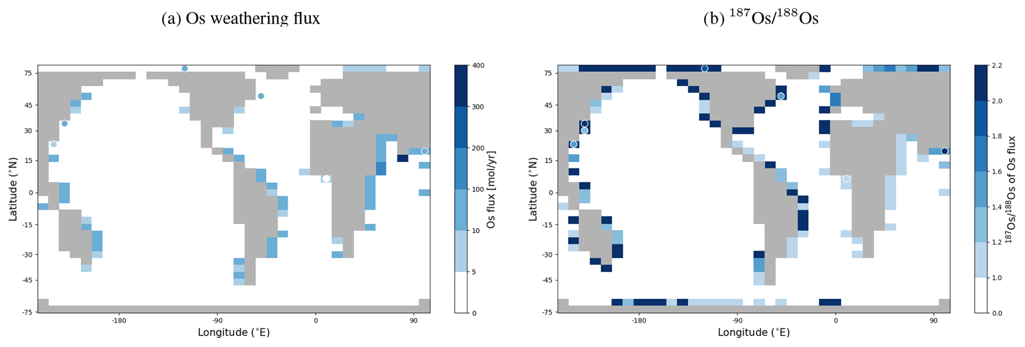
Figure A1Spatially explicit Os weathering flux using the ROKGEM 2D weathering scheme “GEM_CO2” and observed Os river fluxes (colored dots) based on measured Os concentrations (a) and their isotopic composition (b) in rivers (Levasseur et al., 1999) and annual river runoff (Milliman and Farnsworth, 2013).
A2 Marine Os sequestration by association with POC
Another possible explanation for the wider range of observed compared with simulated Os concentrations and isotopic ratios in seawater is spatially-variable Os burial rates. The inclusion of Os cycling in cGENIE enables for the first time the simulation of the effects of heterogeneous marine biogeochemistry on Os burial. As part of the Os cycle implementation, we included options for simulating enhanced Os burial in suboxic settings and Os scavenging by POC in cGENIE, since it is assumed that low oxygen concentrations and/or burial of organic matter intensify Os sequestration (Lu et al., 2017), although rates and exact mechanisms are still uncertain. Here, we present an alteration of the previously presented spin-up of the pre-industrial Os cycle by including enhanced Os deposition via association with POC in sub-oxic conditions and scaled this sink to account for 50 % of marine Os burial (see parameter choices in Table A1).
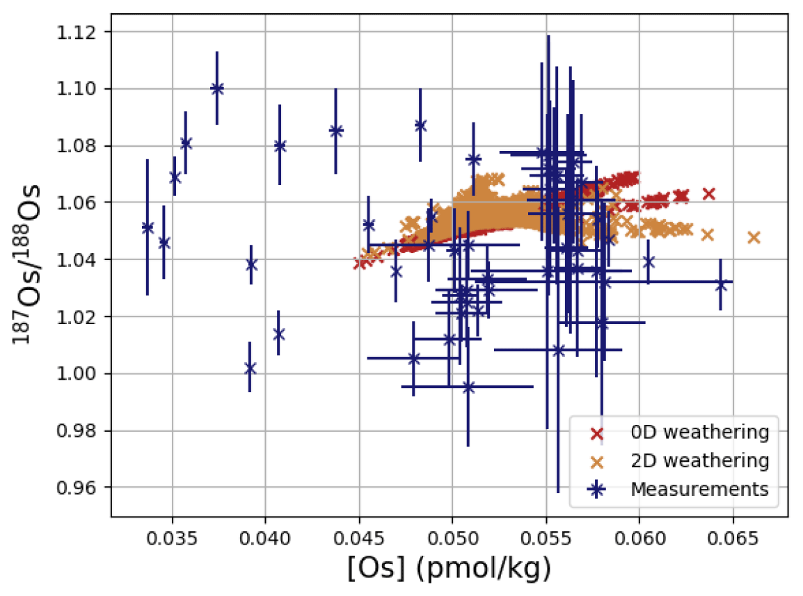
Figure A2Cross plot of measured and simulated Os concentrations and isotopic compositions in seawater, comparing the modern ocean measurements against every ocean grid cell for spin-ups using both the 0D and 2D weathering schemes.
Spatially variable Os burial rates increase the range of simulated Os concentrations in seawater beyond that observed (Fig. A3). While we found that the previous range of simulated Os concentrations covered only half of the observed range, we cannot assess if the lowest simulated Os concentrations with sub-oxic Os scavenging are realistic for the pre-industrial ocean, since only a few Os measurements from oxygen-poor water masses with high POC fluxes are available. However, the range of measured isotopic compositions of Os in seawater is also not reproduced by including spatially variable Os burial. Further modeling and Os measurements in diverse marine settings are urgently needed to address these discrepancies.
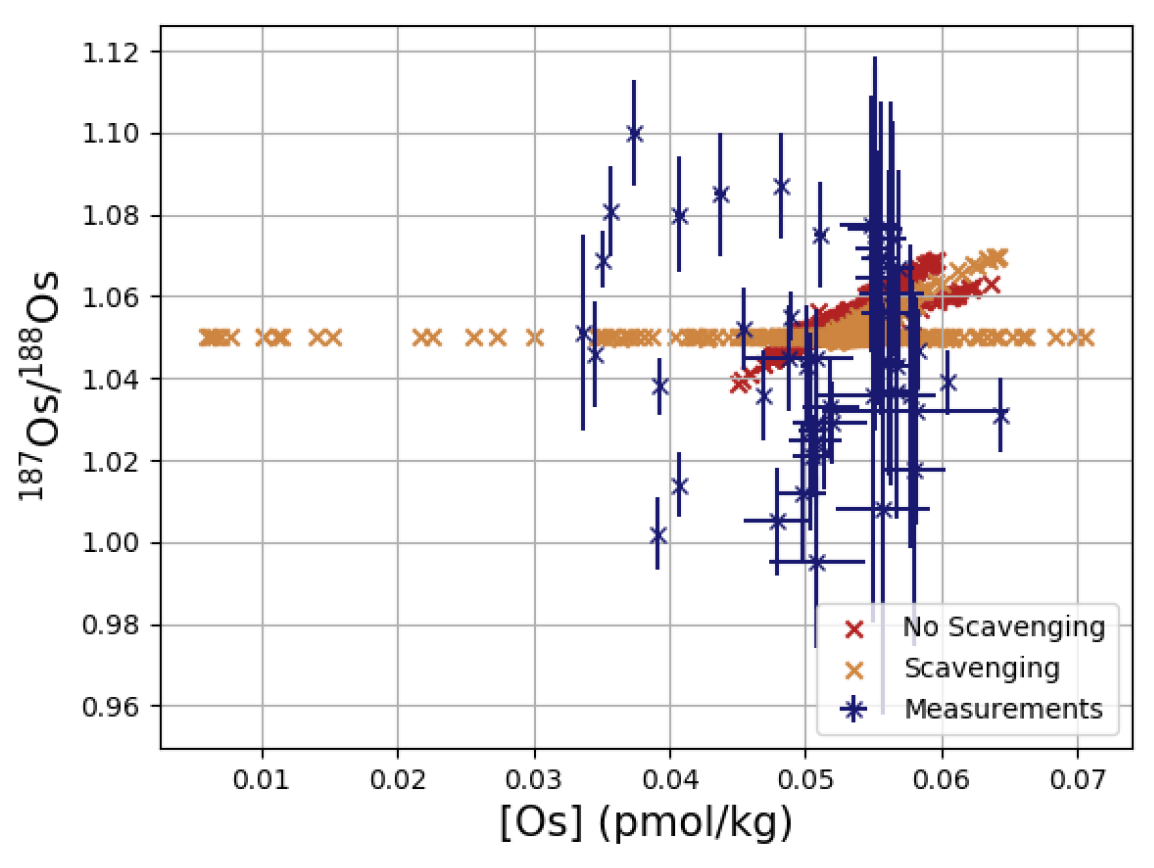
Figure A3Cross plot of measured and simulated Os concentrations and isotopic compositions in seawater with and without Os scavenging under sub-oxic conditions.
A3 Marine signal of large C injections with O2-sensitive Os scavenging
We tested the implications of dynamic Os scavenging on the isotopic response of the marine Os reservoir to climate change by repeating the previously shown C injection simulations with the Os scavenging scheme.
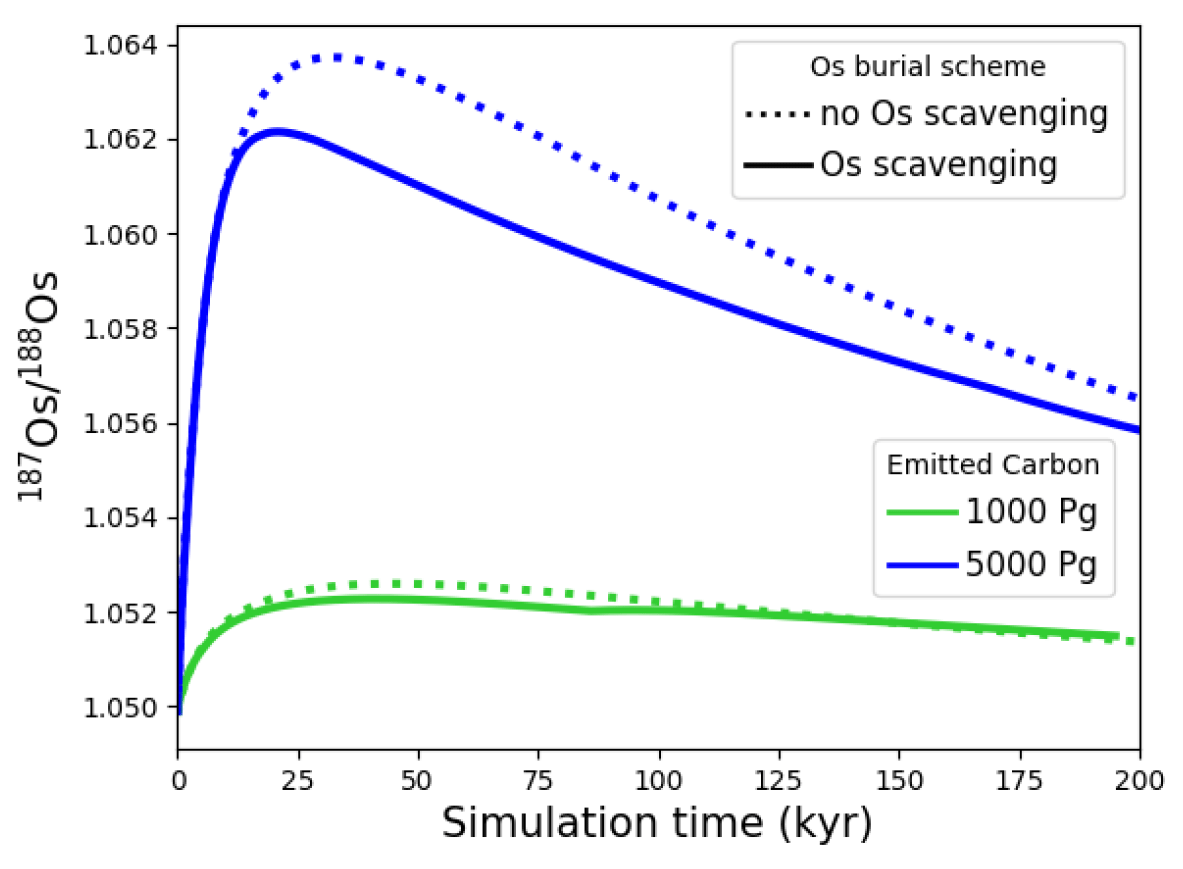
Figure A4Time series of marine changes in response to an immediate release of two different masses of C into the atmosphere–ocean system with and without Os scavenging from the water column
Figure A4 shows that the inclusion of Os scavenging from O2-poor water masses only results in small changes to the simulated evolution of in the C injection experiments. Enhanced remineralization of particulate organic matter in the warmer ocean overcompensates for the effects of reduced marine oxygenation and leads to less Os scavenging and hence a transient growth of the marine Os reservoir. Because the marine Os reservoir grows larger in the simulation with Os scavenging than in the simulation without Os scavenging, the amplitude of the isotopic excursion is smaller.
The abundance and isotopic composition of riverine Li depends primarily on the weathering regime and temperature during clay formation and not on the host lithology (Pogge von Strandmann et al., 2020). Simulations of continental Li fluxes based on rock weathering rates alone therefore do not capture the full variability of the Li cycle under climate change if the latter shifts the weathering regime. ROKGEM does not provide a detailed land surface model, but we included the first-order approximations of the sensitivity of continental Li fluxes on the weathering regime and temperature described in Sect. 3. Here, we show the different simulated response of the marine Li reservoir to a transient warming event with and without these approximations. For this purpose, we repeated the C injection experiments with the optional dependence of continental Li fluxes on the ratio of chemical to physical weathering rates and temperature.

Figure B1Time series of marine δ7Li changes in response to an immediate release of two different amounts of C into the atmosphere–ocean system with and without effects of the ratio of weathering to denudation rate () and temperature on the composition of riverine Li.
Figure B1 shows that appreciable isotopic changes in the marine Li reservoir are only simulated if the continental Li flux changes with changing and temperature. In the simulation with the larger C release, a sudden temperature increase, +7 ∘C at the peak and +3 ∘C sustained for almost 100 kyr, resulted in a marine negative δ7Li excursion of −3 ‰. Although our simulation is set up to represent pre-industrial metal cycles, this amplitude is at the lower end of δ7Li excursions recorded during the Paleocene–Eocene Thermal Maximum, a past C injection event with a similar global mean temperature change (Gehler et al., 2016; Pogge von Strandmann et al., 2019a). cGENIE provides the necessary functionalities to further investigate this and other past δ7Li excursions by enabling the user to prescribe and test early Eocene constraints on the Li cycle, including baseline weathering regimes and rates, the scale of marine clay and evaporite formation and hydrothermal inputs, and the Li concentration in seawater.

Figure C1Cross plot of measured and simulated Ca concentrations and isotopic compositions in seawater using different Ca isotope fractionation schemes.
cGENIE contains three different parameterizations for Ca isotope fractionation during carbonate formation. By default, a fixed user-prescribed fractionation factor is applied across the whole ocean. Alternatively, the fractionation factor can be made dependent on the local concentration of carbonate ions (following Gussone et al., 2005 and Komar and Zeebe, 2016) or the local saturation state (following Tang et al., 2008). A detailed discussion of these approaches can be found in Fantle and Ridgwell (2020). Here, we show the effect of these schemes on the simulated distribution of in pre-industrial seawater and surface sediments.
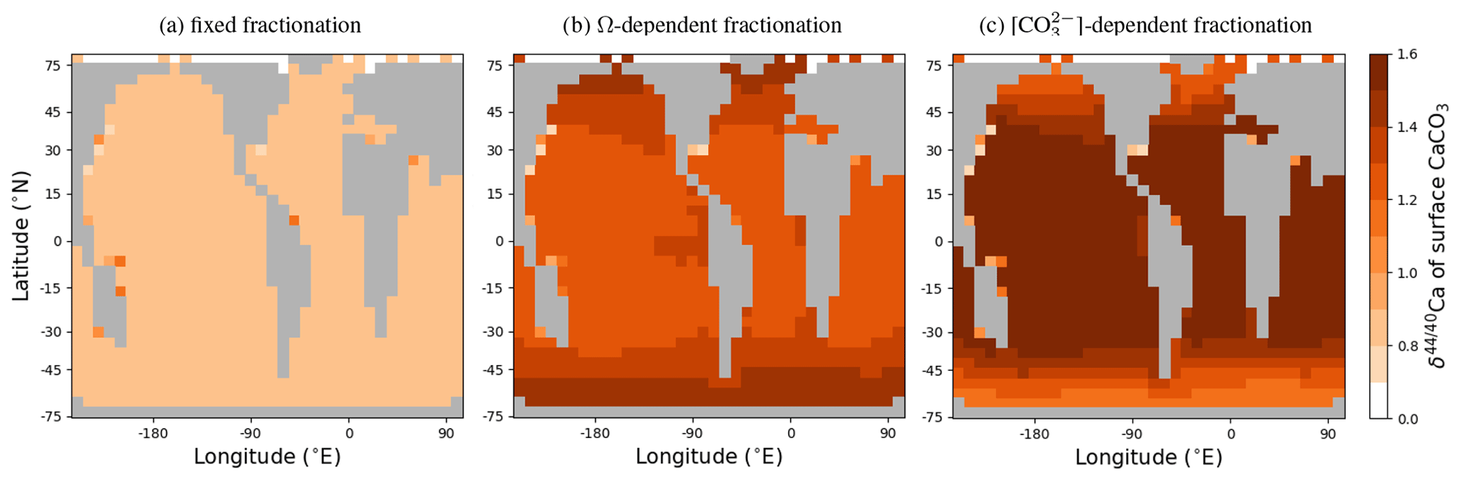
Figure C2The of CaCO3 in the top layer of marine sediments in simulations with different Ca isotope fractionation schemes: (a) fixed fractionation, (b, c) fractionation dependent on local conditions.
We tuned the mean seawater to the same value in all simulations by varying the isotopic composition of continental Ca input, hence the mean composition of seawater aligns in all three simulations but the spatial variability differs. The simulated range of is largest with a fixed fractionation factor because local conditions reduce the fractionation factor across most of the ocean in the simulations with dynamic fractionation factors. The smallest range is simulated when the fractionation factor is dependent on the local concentration of carbonate ions. However, these differences are negligible compared to measurement uncertainty.
In contrast to seawater, the top layer of marine sediments shows substantial differences in in the three simulations (Fig. C2), with generally higher and large spatial variability when the fractionation factor is set by environmental conditions. Sedimentary carbonate is highest at the poles and decreases towards the Equator when the fractionation factor varies with saturation state, while the opposite gradients are simulated using the carbonate-ion-dependent fractionation scheme from Gussone et al. (2005). This illustrates that the surface ocean fractionation factor is shifted in opposing directions by changing carbonate ion abundance in these fractionation schemes Fantle and Ridgwell (2020).
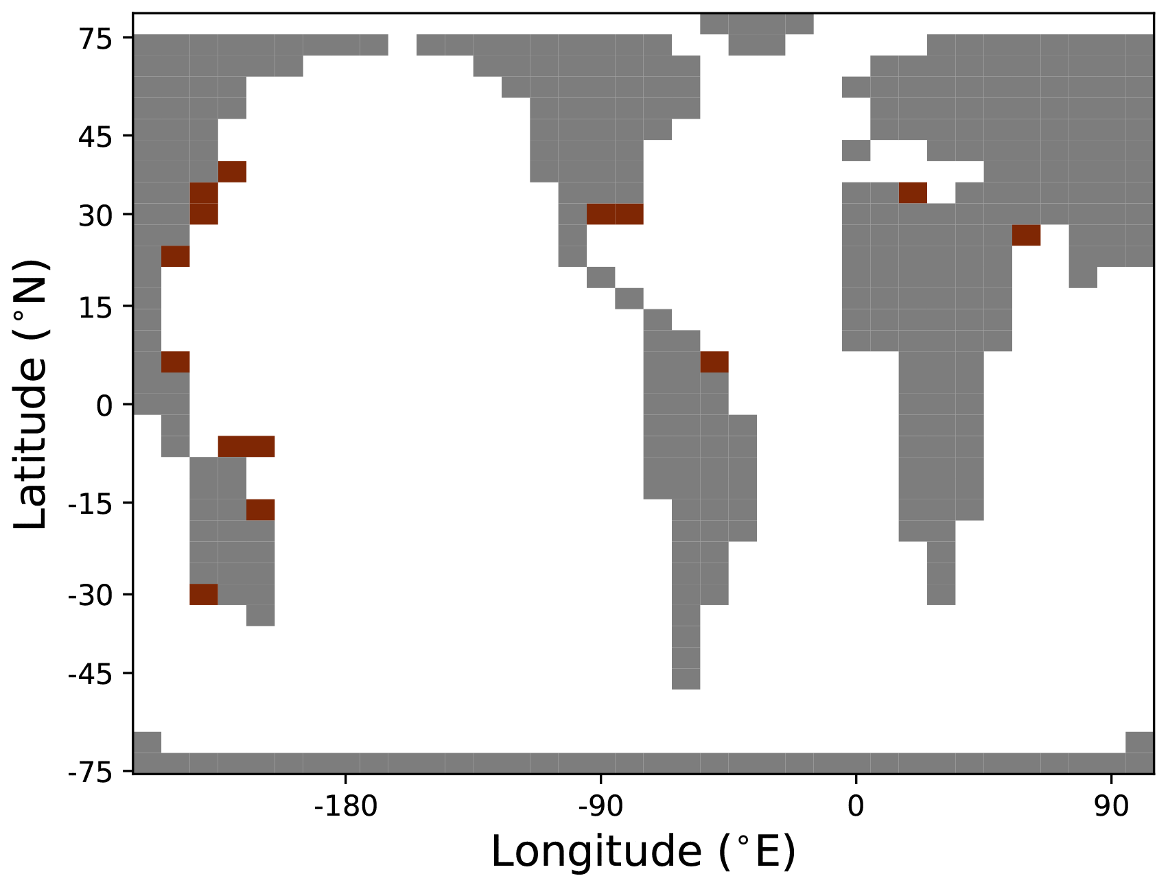
Figure D1Locations with prescribed benthic carbonate deposition representing carbonate reefs. Reef grid cells are highlighted in brown.
Table E1Model parameters setting continental weathering-related trace metal fluxes.

NA: not available.
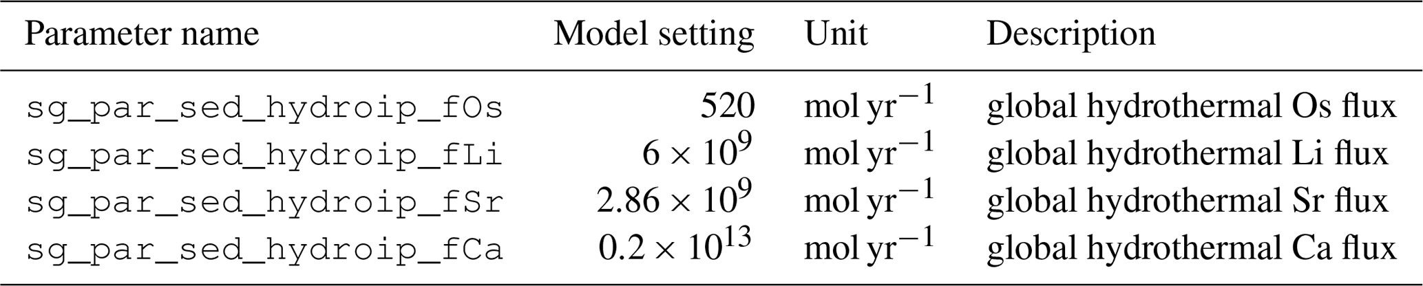
Table E3Model parameters setting the Os, Li and Sr contents of calcite shells.
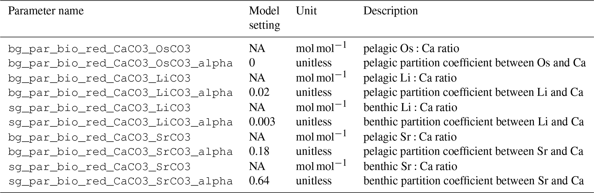
NA: not available.
Table E4Model parameters setting Os scavenging.
NA: not available.
Table E5Model parameters for weathering-related trace metal fluxes.

Table E6Model parameters for Sr recrystallization.
NA: not available.
Table E8Model parameters for the representation of isotopes and isotopic fractionation.
NA: not available.

Figure F1Measured Sr ocean profiles. Composites of all available profiles of measured concentrations (a) and isotopic compositions (b) are shown. Data are taken from Angino et al. (1966), Fabricand et al. (1967), Bernat et al. (1972), Brass and Turekian (1974), De Villiers (1999), Mokadem et al. (2015), and Wakaki et al. (2017). Sr concentrations are normalized to a salinity of 34.90.
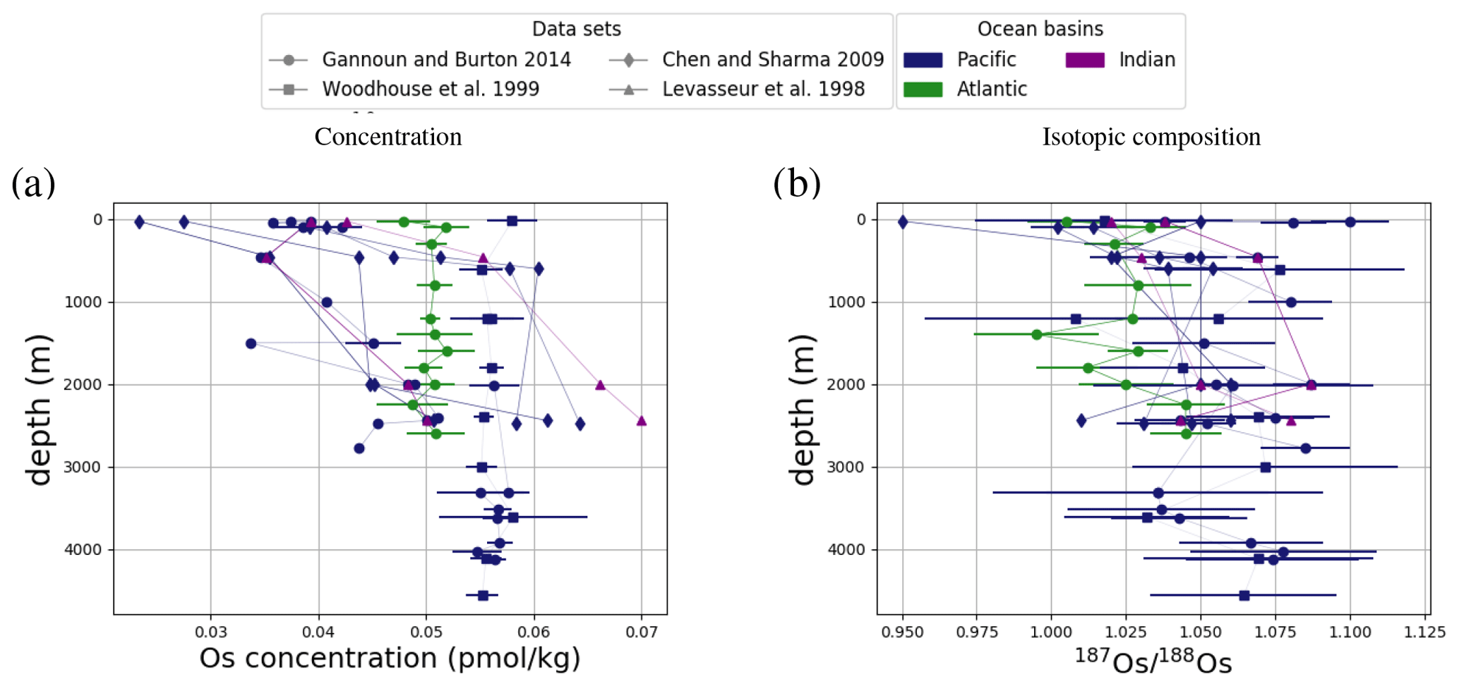
Figure F2Measured Os ocean profiles. Composites of all available profiles of measured concentrations (a) and isotopic compositions (b) are shown. Data are taken from Levasseur et al. (1998), Woodhouse et al. (1999), and Gannoun and Burton (2014).
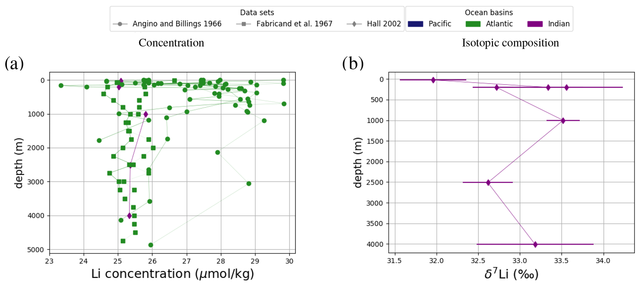
Figure F3Measured Li ocean profiles. Composites of all available profiles of measured concentrations (a) and isotopic compositions (b) are shown. Data are taken from Angino and Billings (1966), Fabricand et al. (1967), Chan (1987), and Hall (2002). Li concentrations are normalized to a salinity of 34.90.
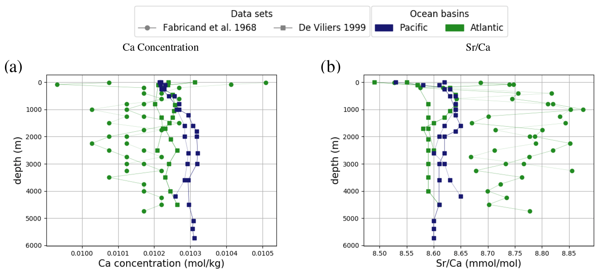
Figure F4Composites of all available ocean Ca concentration (a) and Sr/Ca profiles (b). Data are taken from Fabricand et al. (1967) and De Villiers (1999). Ca concentrations are normalized to a salinity of 34.90.
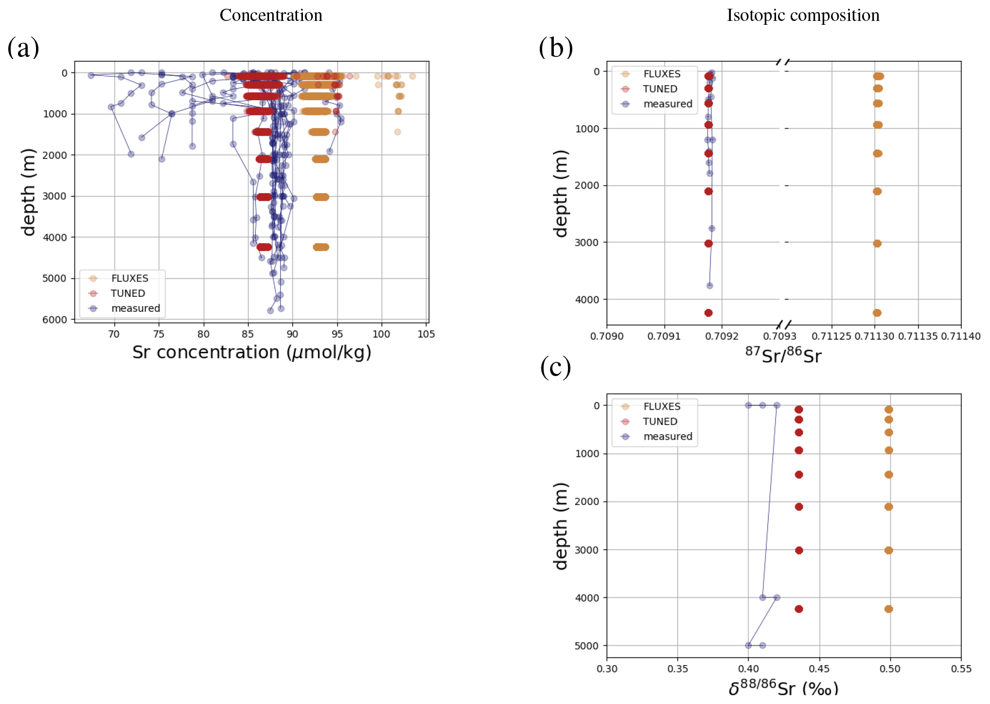
Figure F5Comparison between measured and simulated Sr profiles in seawater. Composites of all available measured Sr concentration (a) and isotope ratio (b, c) profiles and all profiles in the simulation are shown. Data are taken from Angino et al. (1966), Fabricand et al. (1967), Bernat et al. (1972), Brass and Turekian (1974), De Villiers (1999), and Mokadem et al. (2015). Sr concentrations are normalized to a salinity of 34.90.

Figure F6Comparison between measured and simulated Os vertical profiles in seawater. Composites of all available measured Os concentration (a) and isotope ratio (b) profiles and all profiles in the simulation are shown. Data are taken from Levasseur et al. (1998), Woodhouse et al. (1999), and Gannoun and Burton (2014).
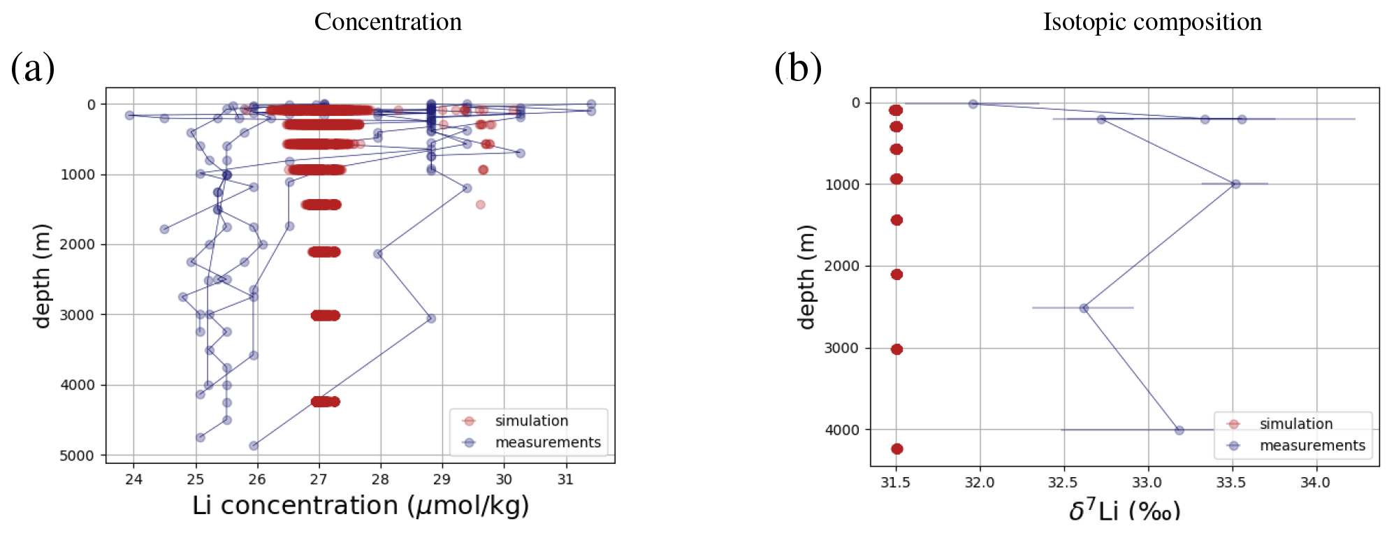
Figure F7Comparison between measured and simulated Li profiles in seawater. Composites of all available measured Li concentration (a) and isotope ratio (b) profiles and all profiles in the simulation are shown. Data are taken from Angino and Billings (1966), Fabricand et al. (1967), Chan (1987), Chan and Edmond (1988), You and Chan (1996), Moriguti and Nakamura (1998), Tomascak et al. (1999), James and Palmer (2000), Košler et al. (2001), Nishio and Nakai (2002), Hall (2002), Bryant et al. (2003), Pistiner and Henderson (2003), Millot et al. (2004), Choi et al. (2010), and Lin et al. (2016). Li concentrations are normalized to a salinity of 34.90.
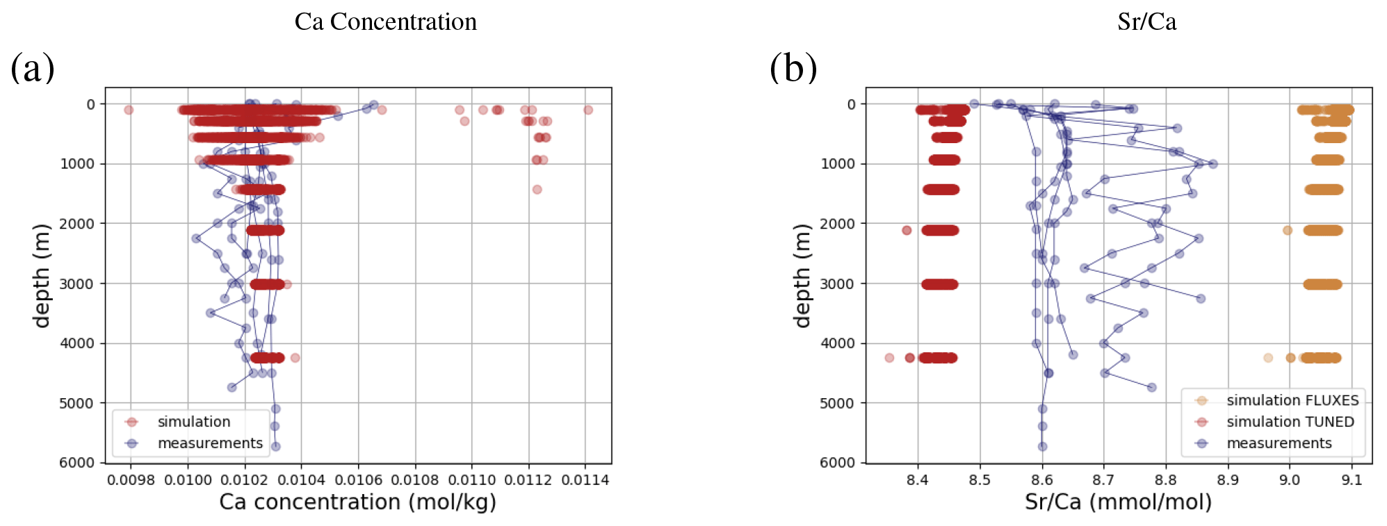
Figure F8Comparison between measured and simulated Ca (a) and (b) profiles in seawater. Composites of all available measured concentration profiles and all profiles in the simulation are shown. Data are taken from Fabricand et al. (1967), De Villiers (1999), and Fantle and Tipper (2014). Ca concentrations are normalized to a salinity of 34.90.

Figure G1Comparison between measured and simulated Sr concentrations (a) and isotopic composition (b, c) in surface waters. Measurements are shown as symbols on the map, with the color indicating the respective value. Data are taken from Angino et al. (1966), Fabricand et al. (1967), Bernat et al. (1972), Brass and Turekian (1974), De Villiers (1999), Mokadem et al. (2015), and Wakaki et al. (2017).
Summary tables of all Sr, Os, Li, and Ca concentration measurements; their locations; and references are provided as separate spreadsheets in the Supplement. Ca isotope ratios in seawater were taken from the compilation in Fantle and Tipper (2014).
The code for the version of the “muffin” release of the cGENIE Earth system model used in this paper is tagged as v0.9.23 and is assigned the following DOI: https://doi.org/10.5281/zenodo.4776445 (Ridgwell et al., 2021a).
Configuration files for the specific experiments presented in the paper can be found in the following directory: genie-userconfigs/MS/adloffetal.GMD.2021. Details of the experiments, plus the command line needed to run each experiment, are given in the readme.txt file in that directory. All other configuration files and boundary conditions are provided as part of the code release.
A manual detailing code installation, basic model configuration, tutorials covering various aspects of model configuration and experimental design, and the results of output and processing is assigned the following DOI: https://doi.org/10.5281/zenodo.4776512 (Ridgwell et al., 2021b).
All observational data have previously been published and are referenced in the figure captions. For convenience, we included spreadsheets with this data compilation in the Supplement to this paper. All scripts to reproduce the model simulations are provided on GitHub (see instructions under Code availability). The model output can also be obtained from Markus Adloff upon request.
The supplement related to this article is available online at: https://doi.org/10.5194/gmd-14-4187-2021-supplement.
The implementation of the Sr, Li and Ca cycles was conceived by AR, PAEPvS and MSF and done by AR. The cGENIE Os cycle was conceived by MA, IJP, AJD and AR and implemented by MA and AR. MA compiled the observational data, validated the model output, and produced the simulations and figures. MA prepared the manuscript with contributions from all co-authors.
The authors declare that they have no conflict of interest.
We thank the two anonymous reviewers and the editor Guy Munhoven for their thorough and constructive reviews, which substantially improved the manuscript. We would also like to thank our funding bodies.
This research has been supported by the Natural Environment Research Council (NERC; grant nos. NE/L002434/1, Markus Adloff; NE/L011050/1 and NE/P01903X/1, Sarah E. Greene; NE/N011112/1, Fanny M. Monteiro), the NERC GW4+ Doctoral Scholarship (Markus Adloff), ERC Consolidator (grant no. 682760, Philip A. E. Pogge von Strandmann), the NSF (grant nos. 1658024 and 1702913), and the Heising Simons Foundation (Andy Ridgwell).
This paper was edited by Guy Munhoven and reviewed by two anonymous referees.
Allègre, C. J., Louvat, P., Gaillardet, J., Meynadier, L., Rad, S., and Capmas, F.: The fundamental role of island arc weathering in the oceanic Sr isotope budget, Earth Planet. Sc. Lett., 292, 51–56, https://doi.org/10.1016/j.epsl.2010.01.019, 2010. a, b
Angino, E. E. and Billings, G. K.: Lithium content of sea water by atomic absorption spectrometry, Geochim. Cosmochim. Ac., 30, 153–158, https://doi.org/10.1016/0016-7037(66)90104-9, 1966. a, b, c, d, e, f, g
Angino, E. E., Billings, G. K., and Andersen, N.: Observed variations in the strontium concentration of sea water, Chem. Geol., 1, 145–153, https://doi.org/10.1016/0009-2541(66)90013-1, 1966. a, b, c, d, e, f, g, h, i
Baskaran, M.: Handbook of environmental isotope geochemistry, Springer Science & Business Media, Berlin, Heidelberg, ISBN: 9783642106361, 2011. a, b
Basu, A. R., Jacobsen, S. B., Poreda, R. J., Dowling, C. B., and Aggarwal, P. K.: Large groundwater strontium flux to the oceans from the Bengal Basin and the marine strontium isotope record, Science, 293, 1470–1473, https://doi.org/10.1126/science.1060524, 2001. a, b
Bauer, K. W., Zeebe, R. E., and Wortmann, U. G.: Quantifying the volcanic emissions which triggered Oceanic Anoxic Event 1a and their effect on ocean acidification, Sedimentology, 64, 204–214, https://doi.org/10.1111/sed.12335, 2017. a
Beck, A. J., Charette, M. A., Cochran, J. K., Gonneea, M. E., and Peucker-Ehrenbrink, B.: Dissolved strontium in the subterranean estuary–implications for the marine strontium isotope budget, Geochim. Cosmochim. Ac., 117, 33–52, https://doi.org/10.1016/j.gca.2013.03.021, 2013. a, b
Bernat, M., Church, T., and Allegre, C. J.: Barium and strontium concentrations in Pacific and Mediterranean sea water profiles by direct isotope dilution mass spectrometry, Earth Planet. Sc. Lett., 16, 75–80, https://doi.org/10.1016/0012-821X(72)90238-5, 1972. a, b, c, d, e
Berner, E. K. and Berner, R. A.: Global environment: water, air, and geochemical cycles, Princeton University Press, Princeton, New Jersey, ISBN: 0691136785, 2012. a, b, c, d
Berner, R.: GEOCARB II: a revised model of atmospheric CO2 levels over Phanerozoic time, Science, 249, 1382–1386, 1994. a
Blättler, C. L., Jenkyns, H. C., Reynard, L. M., and Henderson, G. M.: Significant increases in global weathering during Oceanic Anoxic Events 1a and 2 indicated by calcium isotopes, Earth Planet. Sc. Lett., 309, 77–88, https://doi.org/10.1016/j.epsl.2011.06.029, 2011. a
Blättler, C. L., Henderson, G. M., and Jenkyns, H. C.: Explaining the Phanerozoic Ca isotope history of seawater, Geology, 40, 843–846, https://doi.org/10.1130/G33191.1, 2012. a
Bluth, G. J. and Kump, L. R.: Lithologic and climatologic controls of river chemistry, Geochim. Cosmochim. Ac., 58, 2341–2359, 1994. a
Böhm, F., Eisenhauer, A., Tang, J., Dietzel, M., Krabbenhöft, A., Kisakürek, B., and Horn, C.: Strontium isotope fractionation of planktic foraminifera and inorganic calcite, Geochim. Cosmochim. Ac., 93, 300–314, https://doi.org/10.1016/j.gca.2012.04.038, 2012. a, b
Bottini, C., Cohen, A. S., Erba, E., Jenkyns, H. C., and Coe, A. L.: Osmium-isotope evidence for volcanism, weathering, and ocean mixing during the early Aptian OAE 1a, Geology, 40, 583–586, https://doi.org/10.1130/G33140.1, 2012. a, b
Brady, P. V.: The effect of silicate weathering on global temperature and atmospheric CO2, J. Geophys. Res.-Sol. Ea., 96, 18101–18106, https://doi.org/10.1029/91JB01898, 1991. a
Brady, P. V. and Gíslason, S. R.: Seafloor weathering controls on atmospheric CO2 and global climate, Geochim. Cosmochim. Ac., 61, 965–973, https://doi.org/10.1016/S0016-7037(96)00385-7, 1997. a
Brass, G. W. and Turekian, K. K.: Strontium distribution in GEOSECS oceanic profiles, Earth Planet. Sc. Lett., 23, 141–148, https://doi.org/10.1016/0012-821X(74)90041-7, 1974. a, b, c, d, e
Bryant, C. J., McCulloch, M. T., and Bennett, V. C.: Impact of matrix effects on the accurate measurement of Li isotope ratios by inductively coupled plasma mass spectrometry (MC-ICP-MS) under “cold” plasma conditions, J. Anal. Atom. Spectrom., 18, 734–737, https://doi.org/10.1039/B212083F, 2003. a, b, c
Burton, K. W., Gannoun, A., and Parkinson, I. J.: Climate driven glacial–interglacial variations in the osmium isotope composition of seawater recorded by planktic foraminifera, Earth Planet. Sc. Lett., 295, 58–68, https://doi.org/10.1016/j.epsl.2010.03.026, 2010. a, b, c
Campbell, I. H. and Allen, C. M.: Formation of supercontinents linked to increases in atmospheric oxygen, Nat. Geosci., 1, 554–558, https://doi.org/10.1038/ngeo259, 2008. a
Carignan, J., Cardinal, D., Eisenhauer, A., Galy, A., Rehkamper, M., Wombacher, F., and Vigier, N.: A reflection on Mg, Cd, Ca, Li and Si isotopic measurements and related reference materials, Geostand. Geoanal. Res., 28, 139–148, https://doi.org/10.1111/j.1751-908X.2004.tb01050.x, 2004. a
Chan, L., Edmond, J., Thompson, G., and Gillis, K.: Lithium isotopic composition of submarine basalts: implications for the lithium cycle in the oceans, Earth Planet. Sc. Lett., 108, 151–160, https://doi.org/10.1016/0012-821X(92)90067-6, 1992. a
Chan, L. H.: Lithium isotope analysis by thermal ionization mass spectrometry of lithium tetraborate, Anal. Chem., 59, 2662–2665, https://doi.org/10.1021/ac00149a007, 1987. a, b, c, d
Chan, L.-H. and Edmond, J. M.: Variation of lithium isotope composition in the marine environment: A preliminary report, Geochim. Cosmochim. Ac., 52, 1711–1717, https://doi.org/10.1016/0016-7037(88)90239-6, 1988. a, b, c, d
Choi, M. S., Shin, H. S., and Kil, Y. W.: Precise determination of lithium isotopes in seawater using MC-ICP-MS, Microchem. J., 95, 274–278, https://doi.org/10.1016/j.microc.2009.12.013, 2010. a, b, c
Clergue, C., Dellinger, M., Buss, H., Gaillardet, J., Benedetti, M., and Dessert, C.: Influence of atmospheric deposits and secondary minerals on Li isotopes budget in a highly weathered catchment, Guadeloupe (Lesser Antilles), Chem. Geol., 414, 28–41, https://doi.org/10.1016/j.chemgeo.2015.08.015, 2015. a
Cocker, J., Griffin, B., and Muehlenbachs, K.: Oxygen and carbon isotope evidence for seawater-hydrothermal alteration of the Macquarie Island ophiolite, Earth Planet. Sc. Lett., 61, 112–122, 1982. a
Colbourn, G., Ridgwell, A., and Lenton, T. M.: The Rock Geochemical Model (RokGeM) v0.9, Geosci. Model Dev., 6, 1543–1573, https://doi.org/10.5194/gmd-6-1543-2013, 2013. a, b, c
Coogan, L. A. and Gillis, K. M.: Low-temperature alteration of the seafloor: Impacts on ocean chemistry, Annu. Rev. Earth Pl. Sc., 46, 21–45, 2018. a
Dąbek, J. and Halas, S.: Physical foundations of rhenium-osmium method-a review, Geochronometria, 27, 23–26, https://doi.org/10.2478/v10003-007-0011-4, 2007. a, b
Data Announcement 88-MGG-02: Digital relief of the Surface of the Earth, NOAA, National Geophysical Data Center, Boulder, Colorado, 1988. a
De Villiers, S.: Seawater strontium and Sr/Ca variability in the Atlantic and Pacific oceans, Earth Planet. Sc. Lett., 171, 623–634, https://doi.org/10.1016/S0012-821X(99)00174-0, 1999. a, b, c, d, e, f, g, h, i, j
Death, R., Wadham, J. L., Monteiro, F., Le Brocq, A. M., Tranter, M., Ridgwell, A., Dutkiewicz, S., and Raiswell, R.: Antarctic ice sheet fertilises the Southern Ocean, Biogeosciences, 11, 2635–2643, https://doi.org/10.5194/bg-11-2635-2014, 2014. a
Dellinger, M., Gaillardet, J., Bouchez, J., Calmels, D., Louvat, P., Dosseto, A., Gorge, C., Alanoca, L., and Maurice, L.: Riverine Li isotope fractionation in the Amazon River basin controlled by the weathering regimes, Geochim. Cosmochim. Ac., 164, 71–93, https://doi.org/10.1016/j.gca.2015.04.042, 2015. a, b, c, d
Dellinger, M., West, A. J., Paris, G., Adkins, J. F., Pogge von Strandmann, P. A., Ullmann, C. V., Eagle, R. A., Freitas, P., Bagard, M.-L., Ries, J. B., Corsetti, F. A., Perez-Huerta, A., and Kampf, A. R.: The Li isotope composition of marine biogenic carbonates: Patterns and Mechanisms, Geochim. Cosmochim. Ac., 236, 315–335, https://doi.org/10.1016/j.gca.2018.03.014, 2018. a
DePaolo, D. J.: Calcium isotopic variations produced by biological, kinetic, radiogenic and nucleosynthetic processes, Reviews in Mineralogy and Geochemistry, 55, 255–288, https://doi.org/10.2138/gsrmg.55.1.255, 2004. a
DePaolo, D. J.: Surface kinetic model for isotopic and trace element fractionation during precipitation of calcite from aqueous solutions, Geochim. Cosmochim. Ac., 75, 1039–1056, https://doi.org/10.1016/j.gca.2010.11.020, 2011. a, b
Derry, L. A.: Geochemistry: A glacial hangover, Nature, 458, 417–418, https://doi.org/10.1038/458417a, 2009. a
Dickson, A. J., Cohen, A. S., Coe, A. L., Davies, M., Shcherbinina, E. A., and Gavrilov, Y. O.: Evidence for weathering and volcanism during the PETM from Arctic Ocean and Peri-Tethys osmium isotope records, Palaeogeogr. Palaeocl., 438, 300–307, https://doi.org/10.1016/j.palaeo.2015.08.019, 2015. a
Dubin, A. and Peucker-Ehrenbrink, B.: The importance of organic-rich shales to the geochemical cycles of rhenium and osmium, Chem. Geol., 403, 111–120, https://doi.org/10.1016/j.chemgeo.2015.03.010, 2015. a, b
Edwards, N. R. and Marsh, R.: Uncertainties due to transport-parameter sensitivity in an efficient 3-D ocean-climate model, Clim. Dynam., 24, 415–433, https://doi.org/10.1007/s00382-004-0508-8, 2005. a
Elderfield, H.: Strontium isotope stratigraphy, Palaeogeogr. Palaeocl., 57, 71–90, https://doi.org/10.1016/0031-0182(86)90007-6, 1986. a
Elderfield, H. and Gieskes, J. M.: Sr isotopes in interstitial waters of marine sediments from Deep Sea Drilling Project cores, Nature, 300, 493–497, https://doi.org/10.1038/300493a0, 1982. a
Erba, E., Bottini, C., Weissert, H. J., and Keller, C. E.: Calcareous nannoplankton response to surface-water acidification around Oceanic Anoxic Event 1a, Science, 329, 428–432, https://doi.org/10.1126/science.1188886, 2010. a
Fabricand, B., Imbimbo, E., and Brey, M.: Atomic absorption analyses for Ca, Li, Mg, K, Rb, and Sr at two Atlantic Ocean stations, Deep Sea Research and Oceanographic Abstracts, 14, 785–789, https://doi.org/10.1016/S0011-7471(67)80014-7, 1967. a, b, c, d, e, f, g, h, i, j, k, l, m, n
Fantle, M. S. and Ridgwell, A.: Towards an understanding of the Ca isotopic signal related to ocean acidification and alkalinity overshoots in the rock record, Chem. Geol., 547, 119672, https://doi.org/10.1016/j.chemgeo.2020.119672, 2020. a, b, c
Fantle, M. S. and Tipper, E. T.: Calcium isotopes in the global biogeochemical Ca cycle: Implications for development of a Ca isotope proxy, Earth-Sci. Rev., 129, 148–177, https://doi.org/10.1016/j.earscirev.2013.10.004, 2014. a, b, c, d, e, f, g, h, i, j, k, l, m, n
Fantle, M. S., Tollerud, H., Eisenhauer, A., and Holmden, C.: The Ca isotopic composition of dust-producing regions: Measurements of surface sediments in the Black Rock Desert, Nevada, Geochim. Cosmochim. Ac., 87, 178–193, https://doi.org/10.1016/j.gca.2012.03.037, 2012. a
Fantle, M. S., Barnes, B. D., and Lau, K. V.: The Role of Diagenesis in Shaping the Geochemistry of the Marine Carbonate Record, Annu. Rev. Earth Pl. Sc., 48, 549–583, https://doi.org/10.1146/annurev-earth-073019-060021, 2020. a, b
Farkaš, J., Böhm, F., Wallmann, K., Blenkinsop, J., Eisenhauer, A., Van Geldern, R., Munnecke, A., Voigt, S., and Veizer, J.: Calcium isotope record of Phanerozoic oceans: Implications for chemical evolution of seawater and its causative mechanisms, Geochim. Cosmochim. Ac., 71, 5117–5134, https://doi.org/10.1016/j.gca.2007.09.004, 2007. a, b
Faure, G. and Mensing, T. M.: Isotopes: principles and applications, Wiley-Blackwell Hoboken, New Jersey, ISBN: 0471384372, 2005. a, b, c, d
Fietzke, J. and Eisenhauer, A.: Determination of temperature-dependent stable strontium isotope () fractionation via bracketing standard MC-ICP-MS, Geochem. Geophy. Geosy., 7, https://doi.org/10.1029/2006GC001243, 2006. a, b, c
Finlay, A. J., Selby, D., and Gröcke, D. R.: Tracking the Hirnantian glaciation using Os isotopes, Earth Planet. Sc. Lett., 293, 339–348, https://doi.org/10.1016/j.epsl.2010.02.049, 2010. a
Fries, D. M., James, R. H., Dessert, C., Bouchez, J., Beaumais, A., and Pearce, C. R.: The response of Li and Mg isotopes to rain events in a highly-weathered catchment, Chem. Geol., 519, 68–82, https://doi.org/10.1016/j.chemgeo.2019.04.023, 2019. a, b
Gannoun, A. and Burton, K. W.: High precision osmium elemental and isotope measurements of North Atlantic seawater, J. Anal. Atom. Spectrom., 29, 2330–2342, https://doi.org/10.1039/C4JA00265B, 2014. a, b, c, d, e, f
Gehler, A., Gingerich, P. D., and Pack, A.: Temperature and atmospheric CO2 concentration estimates through the PETM using triple oxygen isotope analysis of mammalian bioapatite, P. Natl. Acad. Sci. USA, 113, 7739–7744, 2016. a
Georg, R., West, A., Vance, D., Newman, K., and Halliday, A. N.: Is the marine osmium isotope record a probe for CO2 release from sedimentary rocks?, Earth Planet. Sc. Lett., 367, 28–38, https://doi.org/10.1016/j.epsl.2013.02.018, 2013. a, b, c, d, e
Gibbs, M. T. and Kump, L. R.: Global chemical erosion during the last glacial maximum and the present: sensitivity to changes in lithology and hydrology, Paleoceanography, 9, 529–543, 1994. a
Gibbs, M. T., Bluth, G. J., Fawcett, P. J., and Kump, L. R.: Global chemical erosion over the last 250 My; variations due to changes in paleogeography, paleoclimate, and paleogeology, Am. J. Sci., 299, 611–651, 1999. a
Goddéris, Y. and François, L.: The Cenozoic evolution of the strontium and carbon cycles: relative importance of continental erosion and mantle exchanges, Chem. Geol., 126, 169–190, https://doi.org/10.1016/0009-2541(95)00117-3, 1995. a
Goldschmidt, V. M.: Der Stoffwechsel der Erde, Z. Elektrochem. Angew. P., 28, 411–421, 1922. a
Gou, L.-F., Jin, Z., Pogge von Strandmann, P. A., Li, G., Qu, Y.-X., Xiao, J., Deng, L., and Galy, A.: Li isotopes in the middle Yellow River: Seasonal variability, sources and fractionation, Geochim. Cosmochim. Ac., 248, 88–108, https://doi.org/10.1016/j.gca.2019.01.007, 2019. a, b, c
Griffith, E. M., Paytan, A., Caldeira, K., Bullen, T. D., and Thomas, E.: A dynamic marine calcium cycle during the past 28 million years, Science, 322, 1671–1674, https://doi.org/10.1126/science.1163614, 2008. a
Gussone, N., Böhm, F., Eisenhauer, A., Dietzel, M., Heuser, A., Teichert, B. M., Reitner, J., Wörheide, G., and Dullo, W.-C.: Calcium isotope fractionation in calcite and aragonite, Geochim. Cosmochim. Ac., 69, 4485–4494, 2005. a, b, c
Hall, J. M.: Barium and lithium in foraminifera: Glacial-interglacial changes in the North Atlantic, LSU Doctoral Dissertations, State University, Louisiana, 2002. a, b, c, d, e, f, g, h
Hall, J. M. and Chan, L.-H.: in multiple species of benthic and planktonic foraminifera: thermocline, latitudinal, and glacial-interglacial variation, Geochim. Cosmochim. Ac., 68, 529–545, https://doi.org/10.1016/S0016-7037(03)00451-4, 2004. a
Hall, J. M., Chan, L.-H., McDonough, W. F., and Turekian, K. K.: Determination of the lithium isotopic composition of planktic foraminifera and its application as a paleo-seawater proxy, Mar. Geol., 217, 255–265, https://doi.org/10.1016/j.margeo.2004.11.015, 2005. a
Hathorne, E. C. and James, R. H.: Temporal record of lithium in seawater: A tracer for silicate weathering?, Earth Planet. Sc. Lett., 246, 393–406, https://doi.org/10.1016/j.epsl.2006.04.020, 2006. a, b, c, d, e, f, g, h, i
Henchiri, S., Gaillardet, J., Dellinger, M., Bouchez, J., and Spencer, R. G.: Riverine dissolved lithium isotopic signatures in low-relief central Africa and their link to weathering regimes, Geophys. Res. Lett., 43, 4391–4399, https://doi.org/10.1002/2016GL067711, 2016. a, b
Heuser, A., Eisenhauer, A., Gussone, N., Bock, B., Hansen, B., and Nägler, T. F.: Measurement of calcium isotopes (δ44Ca) using a multicollector TIMS technique, Int. J. Mass Spectrom., 220, 385–397, https://doi.org/10.1016/S1387-3806(02)00838-2, 2002. a
Hindshaw, R. S., Reynolds, B. C., Wiederhold, J. G., Kiczka, M., Kretzschmar, R., and Bourdon, B.: Calcium isotope fractionation in alpine plants, Biogeochemistry, 112, 373–388, https://doi.org/10.1007/s10533-012-9732-1, 2013. a
Hindshaw, R. S., Tosca, R., Goût, T. L., Farnan, I., Tosca, N. J., and Tipper, E. T.: Experimental constraints on Li isotope fractionation during clay formation, Geochim. Cosmochim. Ac., 250, 219–237, https://doi.org/10.1016/j.gca.2019.02.015, 2019. a, b, c
Hodell, D. A., Mueller, P. A., McKenzie, J. A., and Mead, G. A.: Strontium isotope stratigraphy and geochemistry of the late Neogene ocean, Earth Planet. Sc. Lett., 92, 165–178, https://doi.org/10.1016/0012-821X(89)90044-7, 1989. a
Hodell, D. A., Mead, G. A., and Mueller, P. A.: Variation in the strontium isotopic composition of seawater (8 Ma to present): Implications for chemical weathering rates and dissolved fluxes to the oceans, Chemical Geology: Isotope Geoscience section, 80, 291–307, https://doi.org/10.1016/0168-9622(90)90011-Z, 1990. a
Holmden, C., Papanastassiou, D., Blanchon, P., and Evans, S.: Ca variability in shallow water carbonates and the impact of submarine groundwater discharge on Ca-cycling in marine environments, Geochim. Cosmochim. Ac., 83, 179–194, https://doi.org/10.1016/j.gca.2011.12.031, 2012. a, b, c, d, e, f
Hooper, J., Mayewski, P., Marx, S., Henson, S., Potocki, M., Sneed, S., Handley, M., Gassó, S., Fischer, M., and Saunders, K. M.: Examining links between dust deposition and phytoplankton response using ice cores, Aeolian Res., 36, 45–60, https://doi.org/10.1016/j.aeolia.2018.11.001, 2019. a
Huh, Y., Chan, L.-H., Zhang, L., and Edmond, J. M.: Lithium and its isotopes in major world rivers: implications for weathering and the oceanic budget, Geochim. Cosmochim. Ac., 62, 2039–2051, https://doi.org/10.1016/S0016-7037(98)00126-4, 1998. a
Hülse, D., Arndt, S., and Ridgwell, A.: Mitigation of extreme Ocean Anoxic Event conditions by organic matter sulfurization, Paleoceanography and Paleoclimatology, 34, 476–489, https://doi.org/10.1029/2018PA003470, 2019. a
Jaffe, L. A., Peucker-Ehrenbrink, B., and Petsch, S. T.: Mobility of rhenium, platinum group elements and organic carbon during black shale weathering, Earth Planet. Sc. Lett., 198, 339–353, https://doi.org/10.1016/S0012-821X(02)00526-5, 2002. a
James, R. H. and Palmer, M. R.: The lithium isotope composition of international rock standards, Chem. Geol., 166, 319–326, https://doi.org/10.1016/S0009-2541(99)00217-X, 2000. a, b, c
Jenkyns, H. C.: Geochemistry of oceanic anoxic events, Geochem. Geophy. Geosy., 11, Q03004, https://doi.org/10.1029/2009GC002788, 2010. a
John, E. H., Wilson, J. D., Pearson, P. N., and Ridgwell, A.: Temperature-dependent remineralization and carbon cycling in the warm Eocene oceans, Palaeogeogr. Palaeocl., 413, 158–166, https://doi.org/10.1016/j.palaeo.2014.05.019, 2014. a
Kasemann, S. A., Hawkesworth, C. J., Prave, A. R., Fallick, A. E., and Pearson, P. N.: Boron and calcium isotope composition in Neoproterozoic carbonate rocks from Namibia: evidence for extreme environmental change, Earth Planet. Sc. Lett., 231, 73–86, https://doi.org/10.1016/j.epsl.2004.12.006, 2005. a
Kasemann, S. A., Schmidt, D. N., Pearson, P. N., and Hawkesworth, C. J.: Biological and ecological insights into Ca isotopes in planktic foraminifers as a palaeotemperature proxy, Earth Planet. Sc. Lett., 271, 292–302, https://doi.org/10.1016/j.epsl.2008.04.007, 2008. a, b
Kasemann, S. A., Pogge von Strandmann, P. A., Prave, A. R., Fallick, A. E., Elliott, T., and Hoffmann, K.-H.: Continental weathering following a Cryogenian glaciation: Evidence from calcium and magnesium isotopes, Earth Planet. Sc. Lett., 396, 66–77, https://doi.org/10.1016/j.epsl.2014.03.048, 2014. a, b
Kent, D. V. and Muttoni, G.: Modulation of Late Cretaceous and Cenozoic climate by variable drawdown of atmospheric pCO2 from weathering of basaltic provinces on continents drifting through the equatorial humid belt, Clim. Past, 9, 525–546, https://doi.org/10.5194/cp-9-525-2013, 2013. a
Kirtland Turner, S. and Ridgwell, A.: Recovering the true size of an Eocene hyperthermal from the marine sedimentary record, Paleoceanography, 28, 700–712, 2013. a
Kısakűrek, B., James, R. H., and Harris, N. B.: Li and δ7Li in Himalayan rivers: proxies for silicate weathering?, Earth Planet. Sc. Lett., 237, 387–401, https://doi.org/10.1016/j.epsl.2005.07.019, 2005. a, b
Komar, N. and Zeebe, R.: Calcium and calcium isotope changes during carbon cycle perturbations at the end-Permian, Paleoceanography, 31, 115–130, 2016. a
Košler, J., Kučera, M., and Sylvester, P.: Precise measurement of Li isotopes in planktonic foraminiferal tests by quadrupole ICPMS, Chem. Geol., 181, 169–179, https://doi.org/10.1016/S0009-2541(01)00280-7, 2001. a, b, c
Krabbenhöft, A.: Stable Strontium Isotope (Sr) Fractionation in the Marine Realm: A Pilot Study, PhD thesis, Christian-Albrechts Universität Kiel, Germany, 2011. a
Krabbenhöft, A., Eisenhauer, A., Böhm, F., Vollstaedt, H., Fietzke, J., Liebetrau, V., Augustin, N., Peucker-Ehrenbrink, B., Müller, M., Horn, C., Hansen, B. T., Nolte, N., and Wallmann, K.: Constraining the marine strontium budget with natural strontium isotope fractionations (, ) of carbonates, hydrothermal solutions and river waters, Geochim. Cosmochim. Ac., 74, 4097–4109, https://doi.org/10.1016/j.gca.2010.04.009, 2010. a, b, c, d
Krissansen-Totton, J. and Catling, D. C.: Constraining climate sensitivity and continental versus seafloor weathering using an inverse geological carbon cycle model, Nat. Commun., 8, 1–15, https://doi.org/10.1038/ncomms15423, 2017. a, b
Kristall, B., Jacobson, A. D., and Hurtgen, M. T.: Modeling the paleo-seawater radiogenic strontium isotope record: A case study of the Late Jurassic-Early Cretaceous, Palaeogeogr. Palaeocl., 472, 163–176, https://doi.org/10.1016/j.palaeo.2017.01.048, 2017. a, b, c, d, e, f, g, h
Kump, L. R. and Barley, M. E.: Increased subaerial volcanism and the rise of atmospheric oxygen 2.5 billion years ago, Nature, 448, 1033, https://doi.org/10.1038/nature06058, 2007. a
Lechler, M., Pogge von Strandmann, P. A., Jenkyns, H. C., Prosser, G., and Parente, M.: Lithium-isotope evidence for enhanced silicate weathering during OAE 1a (Early Aptian Selli event), Earth Planet. Sc. Lett., 432, 210–222, 2015. a
Lemarchand, E., Chabaux, F., Vigier, N., Millot, R., and Pierret, M.-C.: Lithium isotope systematics in a forested granitic catchment (Strengbach, Vosges Mountains, France), Geochim. Cosmochim. Ac., 74, 4612–4628, https://doi.org/10.1016/j.gca.2010.04.057, 2010. a
Lenton, T. M., Marsh, R., Price, A. R., Lunt, D. J., Aksenov, Y., Annan, J. D., Cooper-Chadwick, T., Cox, S. J., Edwards, N. R., Goswami, S., Hargreaves, J. C., Harris, P. P., Jiao, Z., Livina, V. N., Payne, A. J., Rutt, I. C., Shepherd, J. G., Valdes, P. J., Williams, G., Williamson, M. S., and Yool, A.: Effects of atmospheric dynamics and ocean resolution on bi-stability of the thermohaline circulation examined using the Grid ENabled Integrated Earth system modelling (GENIE) framework, Clim. Dynam., 29, 591–613, 2007. a
Levasseur, S., Birck, J.-L., and Allègre, C. J.: Direct measurement of femtomoles of osmium and the ratio in seawater, Science, 282, 272–274, https://doi.org/10.1126/science.282.5387.272, 1998. a, b, c, d, e
Levasseur, S., Birck, J.-L., and Allegre, C.: The osmium riverine flux and the oceanic mass balance of osmium, Earth Planet. Sc. Lett., 174, 7–23, 1999. a
Li, G., Ji, J., Chen, J., and Kemp, D. B.: Evolution of the Cenozoic carbon cycle: The roles of tectonics and CO2 fertilization, Global Biogeochem. Cy., 23, GB1009, https://doi.org/10.1029/2008GB003220, 2009. a
Lin, J., Liu, Y., Hu, Z., Yang, L., Chen, K., Chen, H., Zong, K., and Gao, S.: Accurate determination of lithium isotope ratios by MC-ICP-MS without strict matrix-matching by using a novel washing method, J. Anal. Atom. Spectrom., 31, 390–397, https://doi.org/10.1039/C5JA00231A, 2016. a, b, c
Lord, N. S., Ridgwell, A., Thorne, M., and Lunt, D.: An impulse response function for the “long tail” of excess atmospheric CO2 in an Earth system model, Global Biogeochem. Cy., 30, 2–17, https://doi.org/10.1002/2014GB005074, 2016. a, b, c, d, e
Loveley, M. R., Marcantonio, F., Wisler, M. M., Hertzberg, J. E., Schmidt, M. W., and Lyle, M.: Millennial-scale iron fertilization of the eastern equatorial Pacific over the past 100,000 years, Nature Geoscience, 10, 760–764, https://doi.org/10.1038/ngeo3024, 2017. a
Lu, X., Kendall, B., Stein, H. J., and Hannah, J. L.: Temporal record of osmium concentrations and 187Os/188Os in organic-rich mudrocks: Implications for the osmium geochemical cycle and the use of osmium as a paleoceanographic tracer, Geochim. Cosmochim. Ac., 216, 221–241, https://doi.org/10.1016/j.gca.2017.06.046, 2017. a, b, c, d, e, f, g, h, i, j
Marriott, C. S., Henderson, G. M., Belshaw, N. S., and Tudhope, A. W.: Temperature dependence of δ7Li, δ44Ca and during growth of calcium carbonate, Earth Planet. Sc. Lett., 222, 615–624, https://doi.org/10.1016/j.epsl.2004.02.031, 2004. a
Martin, J. H.: Glacial-interglacial CO2 change: The iron hypothesis, Paleoceanography, 5, 1–13, https://doi.org/10.1029/PA005i001p00001, 1990. a
Martínez-Garcia, A., Rosell-Melé, A., Jaccard, S. L., Geibert, W., Sigman, D. M., and Haug, G. H.: Southern Ocean dust–climate coupling over the past four million years, Nature, 476, 312–315, https://doi.org/10.1038/nature10310, 2011. a
Mason, E., Edmonds, M., and Turchyn, A. V.: Remobilization of crustal carbon may dominate volcanic arc emissions, Science, 357, 290–294, https://doi.org/10.1126/science.aan5049, 2017. a
Menzies, M. and Seyfried Jr., W.: Basalt-seawater interaction: trace element and strontium isotopic variations in experimentally altered glassy basalt, Earth Planet. Sc. Lett., 44, 463–472, https://doi.org/10.1016/0012-821X(79)90084-0, 1979. a
Milliman, J. D.: Production and accumulation of calcium carbonate in the ocean: budget of a nonsteady state, Global Biogeochem. Cy., 7, 927–957, https://doi.org/10.1029/93GB02524, 1993. a, b, c
Milliman, J. D. and Farnsworth, K. L.: River discharge to the coastal ocean: a global synthesis, Cambridge University Press, Cambridge University, ISBN: 9780511781247, 2013. a
Millot, R., Guerrot, C., and Vigier, N.: Accurate and high-precision measurement of lithium isotopes in two reference materials by MC-ICP-MS, Geostand. Geoanal. Res., 28, 153–159, https://doi.org/10.1111/j.1751-908X.2004.tb01052.x, 2004. a, b, c
Millot, R., Vigier, N., and Gaillardet, J.: Behaviour of lithium and its isotopes during weathering in the Mackenzie Basin, Canada, Geochim. Cosmochim. Ac., 74, 3897–3912, https://doi.org/10.1016/j.gca.2010.04.025, 2010. a, b
Mills, B., Daines, S. J., and Lenton, T. M.: Changing tectonic controls on the long-term carbon cycle from Mesozoic to present, Geochem. Geophy. Geosy., 15, 4866–4884, https://doi.org/10.1002/2014GC005530, 2014. a
Misra, S. and Froelich, P. N.: Lithium isotope history of Cenozoic seawater: changes in silicate weathering and reverse weathering, Science, 335, 818–823, https://doi.org/10.1126/science.1214697, 2012. a, b, c, d, e, f, g, h, i, j
Mokadem, F., Parkinson, I. J., Hathorne, E. C., Anand, P., Allen, J. T., and Burton, K. W.: High-precision radiogenic strontium isotope measurements of the modern and glacial ocean: Limits on glacial–interglacial variations in continental weathering, Earth Planet. Sc. Lett., 415, 111–120, https://doi.org/10.1016/j.epsl.2015.01.036, 2015. a, b, c, d, e, f
Monteiro, F., Pancost, R., Ridgwell, A., and Donnadieu, Y.: Nutrients as the dominant control on the spread of anoxia and euxinia across the Cenomanian-Turonian oceanic anoxic event (OAE2): Model-data comparison, Paleoceanography, 27, PA4209, https://doi.org/10.1029/2012PA002351, 2012. a
Moriguti, T. and Nakamura, E.: High-yield lithium separation and the precise isotopic analysis for natural rock and aqueous samples, Chem. Geol., 145, 91–104, https://doi.org/10.1016/S0009-2541(97)00163-0, 1998. a, b, c
Müller, M. N., Krabbenhöft, A., Vollstaedt, H., Brandini, F., and Eisenhauer, A.: Stable isotope fractionation of strontium in coccolithophore calcite: Influence of temperature and carbonate chemistry, Geobiology, 16, 297–306, https://doi.org/10.1111/gbi.12276, 2018. a
Murphy, M. J., Porcelli, D., Pogge von Strandmann, P. A., Hirst, C. A., Kutscher, L., Katchinoff, J. A., Mörth, C.-M., Maximov, T., and Andersson, P. S.: Tracing silicate weathering processes in the permafrost-dominated Lena River watershed using lithium isotopes, Geochim. Cosmochim. Ac., 245, 154–171, https://doi.org/10.1016/j.gca.2018.10.024, 2019. a, b, c
Naafs, B. D. A., Monteiro, F. M., Pearson, A., Higgins, M. B., Pancost, R. D., and Ridgwell, A.: Fundamentally different global marine nitrogen cycling in response to severe ocean deoxygenation, P. Natl. Acad. Sci. USA, 116, 24979–24984, 2019. a
Nägler, T. F., Eisenhauer, A., Müller, A., Hemleben, C., and Kramers, J.: The δ44Ca-temperature calibration on fossil and cultured Globigerinoides sacculifer: New tool for reconstruction of past sea surface temperatures, Geochem. Geophy. Geosy., 1, 1052, https://doi.org/10.1029/2000GC000091, 2000. a, b
Nanne, J. A., Millet, M.-A., Burton, K. W., Dale, C. W., Nowell, G. M., and Williams, H. M.: High precision osmium stable isotope measurements by double spike MC-ICP-MS and N-TIMS, J. Anal. Atom. Spectrom., 32, 749–765, https://doi.org/10.1039/C6JA00406G, 2017. a
Nier, A. O.: The isotopic constitution of strontium, barium, bismuth, thallium and mercury, Phys. Rev., 54, 275, https://doi.org/10.1103/PhysRev.54.275, 1938. a
Nishio, Y. and Nakai, S.: Accurate and precise lithium isotopic determinations of igneous rock samples using multi-collector inductively coupled plasma mass spectrometry, Anal. Chim. Acta, 456, 271–281, https://doi.org/10.1016/S0003-2670(02)00042-9, 2002. a, b, c
Oxburgh, R.: Residence time of osmium in the oceans, Geochem. Geophy. Geosy., 2, 1018, https://doi.org/10.1029/2000GC000104, 2001. a, b
Panchuk, K., Ridgwell, A., and Kump, L.: Sedimentary response to Paleocene-Eocene Thermal Maximum carbon release: A model-data comparison, Geology, 36, 315–318, https://doi.org/10.1130/G24474A.1, 2008. a, b
Parkinson, I. J., Hammond, S. J., James, R. H., and Rogers, N. W.: High-temperature lithium isotope fractionation: Insights from lithium isotope diffusion in magmatic systems, Earth Planet. Sc. Lett., 257, 609–621, https://doi.org/10.1016/j.epsl.2007.03.023, 2007. a
Paytan, A., Griffith, E. M., Eisenhauer, A., Hain, M. P., Wallmann, K., and Ridgwell, A.: A 35-million-year record of seawater stable Sr isotopes reveals a fluctuating global carbon cycle, Science, 371, 1346–1350, 2021. a, b
Pearce, C. R., Parkinson, I. J., Gaillardet, J., Charlier, B. L., Mokadem, F., and Burton, K. W.: Reassessing the stable (Sr) and radiogenic () strontium isotopic composition of marine inputs, Geochim. Cosmochim. Ac., 157, 125–146, https://doi.org/10.1016/j.gca.2015.02.029, 2015. a, b, c, d, e, f, g
Penniston-Dorland, S., Liu, X.-M., and Rudnick, R. L.: Lithium isotope geochemistry, Rev. Mineral. Geochem., 82, 165–217, https://doi.org/10.2138/rmg.2017.82.6, 2017. a, b, c
Percival, L., Witt, M., Mather, T., Hermoso, M., Jenkyns, H., Hesselbo, S., Al-Suwaidi, A., Storm, M., Xu, W., and Ruhl, M.: Globally enhanced mercury deposition during the end-Pliensbachian extinction and Toarcian OAE: A link to the Karoo–Ferrar Large Igneous Province, Earth Planet. Sc. Lett., 428, 267–280, https://doi.org/10.1016/j.epsl.2015.06.064, 2015. a
Perez-Fernandez, A., Berninger, U.-N., Mavromatis, V., Pogge von Strandmann, P. A., and Oelkers, E.: Ca and Mg isotope fractionation during the stoichiometric dissolution of dolomite at temperatures from 51 to 126 ∘C and 5 bars CO2 pressure, Chem. Geol., 467, 76–88, https://doi.org/10.1016/j.chemgeo.2017.07.026, 2017. a
Peucker-Ehrenbrink, B. and Jahn, B.-m.: Rhenium-osmium isotope systematics and platinum group element concentrations: Loess and the upper continental crust, Geochem. Geophy. Geosy., 2, 1061, https://doi.org/10.1029/2001GC000172, 2001. a
Peucker-Ehrenbrink, B. and Ravizza, G.: The marine osmium isotope record, Terra Nova, 12, 205–219, https://doi.org/10.1046/j.1365-3121.2000.00295.x, 2000. a
Peucker-Ehrenbrink, B., Ravizza, G., and Hofmann, A.: The marine record of the past 80 million years, Earth Planet. Sc. Lett., 130, 155–167, https://doi.org/10.1016/0012-821X(95)00003-U, 1995. a
Peucker-Ehrenbrink, B., Miller, M. W., Arsouze, T., and Jeandel, C.: Continental bedrock and riverine fluxes of strontium and neodymium isotopes to the oceans, Geochem. Geophy. Geosy., 11, Q03016, https://doi.org/10.1029/2009GC002869, 2010. a, b
Phan, T. T., Capo, R. C., Stewart, B. W., Macpherson, G., Rowan, E. L., and Hammack, R. W.: Factors controlling Li concentration and isotopic composition in formation waters and host rocks of Marcellus Shale, Appalachian Basin, Chem. Geol., 420, 162–179, https://doi.org/10.1016/j.chemgeo.2015.11.003, 2016. a, b
Pistiner, J. S. and Henderson, G. M.: Lithium-isotope fractionation during continental weathering processes, Earth Planet. Sc. Lett., 214, 327–339, https://doi.org/10.1016/S0012-821X(03)00348-0, 2003. a, b, c, d, e
Pogge von Strandmann, P. A. and Henderson, G. M.: The Li isotope response to mountain uplift, Geology, 43, 67–70, https://doi.org/10.1130/G36162.1, 2015. a, b, c, d
Pogge von Strandmann, P. A., Burton, K. W., James, R. H., van Calsteren, P., and Gislason, S. R.: Assessing the role of climate on uranium and lithium isotope behaviour in rivers draining a basaltic terrain, Chem. Geol., 270, 227–239, https://doi.org/10.1016/j.chemgeo.2009.12.002, 2010. a, b
Pogge von Strandmann, P. A., Burton, K. W., Opfergelt, S., Eiríksdóttir, E. S., Murphy, M. J., Einarsson, A., and Gislason, S. R.: The effect of hydrothermal spring weathering processes and primary productivity on lithium isotopes: Lake Myvatn, Iceland, Chem. Geol., 445, 4–13, https://doi.org/10.1016/j.chemgeo.2016.02.026, 2016. a
Pogge von Strandmann, P. A., Frings, P. J., and Murphy, M. J.: Lithium isotope behaviour during weathering in the Ganges Alluvial Plain, Geochim. Cosmochim. Ac., 198, 17–31, https://doi.org/10.1016/j.gca.2016.11.017, 2017. a, b, c
Pogge von Strandmann, P., Jones, M., Schmidt, D., and Murphy, M.: Lithium Isotope Evidence for More Efficient CO2 Drawdown Across the PETM, Goldschmidt Abstracts, 2019a. a
Pogge von Strandmann, P. A., Hendry, K. R., Hatton, J., and Robinson, L.: The response of magnesium, silicon and calcium isotopes to rapidly uplifting and weathering terrains: South Island, New Zealand, Front. Earth Sci., 7, 240, https://doi.org/10.3389/feart.2019.00240, 2019b. a, b, c
Pogge von Strandmann, P. A., Kasemann, S. A., and Wimpenny, J. B.: Lithium and lithium isotopes in Earth’s surface cycles, Elements, 16, 253–258, 2020. a, b, c, d
Racionero-Gómez, B., Sproson, A., Selby, D., Gannoun, A., Gröcke, D., Greenwell, H., and Burton, K. W.: Osmium uptake, distribution, and and compositions in Phaeophyceae macroalgae, Fucus vesiculosus: Implications for determining the composition of seawater, Geochim. Cosmochim. Ac., 199, 48–57, https://doi.org/10.1016/j.gca.2016.11.033, 2017. a
Reinhard, C. T., Olson, S. L., Kirtland Turner, S., Pälike, C., Kanzaki, Y., and Ridgwell, A.: Oceanic and atmospheric methane cycling in the cGENIE Earth system model – release v0.9.14, Geosci. Model Dev., 13, 5687–5706, https://doi.org/10.5194/gmd-13-5687-2020, 2020. a
Richter, E., Hennig, C., Zeimer, U., Weyers, M., Tränkle, G., Reiche, P., Ganschow, S., Uecker, R., and Peters, K.: Freestanding two inch c-plane GaN layers grown on (100) γ-lithium aluminium oxide by hydride vapour phase epitaxy, Phys. Status Solidi (c), 3, 1439–1443, https://doi.org/10.1002/pssc.200565278, 2006. a
Rickaby, R., Schrag, D., Zondervan, I., and Riebesell, U.: Growth rate dependence of Sr incorporation during calcification of Emiliania huxleyi, Global Biogeochem. Cy., 16, 6-1–6-8, https://doi.org/10.1029/2001GB001408, 2002. a
Ridgwell, A. and Hargreaves, J.: Regulation of atmospheric CO2 by deep-sea sediments in an Earth system model, Global Biogeochem. Cy., 21, GB2008, https://doi.org/10.1029/2006GB002764, 2007. a, b, c, d
Ridgwell, A. and Watson, A. J.: Feedback between aeolian dust, climate, and atmospheric CO2 in glacial time, Paleoceanography, 17, 11-1–11-11, 2002. a
Ridgwell, A. and Zeebe, R. E.: The role of the global carbonate cycle in the regulation and evolution of the Earth system, Earth Planet. Sc. Lett., 234, 299–315, https://doi.org/10.1016/j.epsl.2005.03.006, 2005. a, b
Ridgwell, A., Hargreaves, J. C., Edwards, N. R., Annan, J. D., Lenton, T. M., Marsh, R., Yool, A., and Watson, A.: Marine geochemical data assimilation in an efficient Earth System Model of global biogeochemical cycling, Biogeosciences, 4, 87–104, https://doi.org/10.5194/bg-4-87-2007, 2007. a, b, c, d, e, f, g
Ridgwell, A., Reinhard, C., van de Velde, S., Adloff, M., Monteiro, F., Hülse, D., Wilson, J., Ward, B., Vervoort, P., Kirtland Turner, S., and Li, M.: derpycode/cgenie.muffin: Adloff et al. [revised for GMD] (Version v0.9.23), Zenodo [code], https://doi.org/10.5281/zenodo.4776445, 2021a. a
Ridgwell, A., Hülse, D., Peterson, C., Ward, B., sjszas, evansmn, and Jones, R.: derpycode/muffindoc: (Version v0.9.23), Zenodo [code], https://doi.org/10.5281/zenodo.4776512, 2021b. a
Ridgwell, A. J.: Glacial-interglacial perturbations in the global carbon cycle, PhD thesis, University of East Anglia, Norwich, UK, 2001. a
Rollion-Bard, C., Vigier, N., Meibom, A., Blamart, D., Reynaud, S., Rodolfo-Metalpa, R., Martin, S., and Gattuso, J.-P.: Effect of environmental conditions and skeletal ultrastructure on the Li isotopic composition of scleractinian corals, Earth Planet. Sc. Lett., 286, 63–70, https://doi.org/10.1016/j.epsl.2009.06.015, 2009. a
Rosner, M., Ball, L., Peucker-Ehrenbrink, B., Blusztajn, J., Bach, W., and Erzinger, J.: A simplified, accurate and fast method for lithium isotope analysis of rocks and fluids, and δ7Li values of seawater and rock reference materials, Geostand. Geoanal. Res., 31, 77–88, https://doi.org/10.1111/j.1751-908X.2007.00843.x, 2007. a
Rudnick, R. L., Tomascak, P. B., Njo, H. B., and Gardner, L. R.: Extreme lithium isotopic fractionation during continental weathering revealed in saprolites from South Carolina, Chem. Geol., 212, 45–57, https://doi.org/10.1016/j.chemgeo.2004.08.008, 2004. a
Rüggeberg, A., Fietzke, J., Liebetrau, V., Eisenhauer, A., Dullo, W.-C., and Freiwald, A.: Stable strontium isotopes (Sr) in cold-water corals – a new proxy for reconstruction of intermediate ocean water temperatures, Earth Planet. Sc. Lett., 269, 570–575, https://doi.org/10.1016/j.epsl.2008.03.002, 2008. a
Sharma, M., Papanastassiou, D., and Wasserburg, G.: The concentration and isotopic composition of osmium in the oceans, Geochim. Cosmochim. Ac., 61, 3287–3299, https://doi.org/10.1016/S0016-7037(97)00210-X, 1997. a
Sharma, M., Rosenberg, E. J., and Butterfield, D. A.: Search for the proverbial mantle osmium sources to the oceans: Hydrothermal alteration of mid-ocean ridge basalt, Geochim. Cosmochim. Ac., 71, 4655–4667, https://doi.org/10.1016/j.gca.2007.06.062, 2007. a, b, c, d
Sime, N. G., Christina, L., Tipper, E. T., Tripati, A., Galy, A., and Bickle, M. J.: Interpreting the Ca isotope record of marine biogenic carbonates, Geochim. Cosmochim. Ac., 71, 3979–3989, https://doi.org/10.1016/j.gca.2007.06.009, 2007. a
Stevenson, E. I., Hermoso, M., Rickaby, R. E., Tyler, J. J., Minoletti, F., Parkinson, I. J., Mokadem, F., and Burton, K. W.: Controls on stable strontium isotope fractionation in coccolithophores with implications for the marine Sr cycle, Geochim. Cosmochim. Ac., 128, 225–235, https://doi.org/10.1016/j.gca.2013.11.043, 2014. a, b, c, d, e
Stoffyn-Egli, P. and Mackenzie, F. T.: Mass balance of dissolved lithium in the oceans, Geochim. Cosmochim. Ac., 48, 859–872, 1984. a, b
Stoll, H. M. and Schrag, D. P.: Sr/Ca variations in Cretaceous carbonates: relation to productivity and sea level changes, Palaeogeogr. Palaeocl., 168, 311–336, https://doi.org/10.1016/S0031-0182(01)00205-X, 2001. a
Suchet, P. A. and Probst, J.-L.: A global model for present-day atmospheric/soil CO2 consumption by chemical erosion of continental rocks (GEM-CO2), Tellus B, 47, 273–280, 1995. a
Talley, L. D.: Salinity patterns in the ocean, in: The Earth system: physical and chemical dimensions of global environmental change, edited by: MacCracken, M. C., Perry, J. S., and Munn, T., John Wiley & Sons, Ltd Chichester, England, 1, 629–640, 2002. a
Tang, J., Köhler, S. J., and Dietzel, M.: and fractionation during inorganic calcite formation: I. Sr incorporation, Geochim. Cosmochim. Ac., 72, 3718–3732, https://doi.org/10.1016/j.gca.2008.05.033, 2008. a, b, c, d
Tejada, M. L. G., Suzuki, K., Kuroda, J., Coccioni, R., Mahoney, J. J., Ohkouchi, N., Sakamoto, T., and Tatsumi, Y.: Ontong Java Plateau eruption as a trigger for the early Aptian oceanic anoxic event, Geology, 37, 855–858, https://doi.org/10.1130/G25763A.1, 2009. a, b
Them, T. R., Gill, B. C., Selby, D., Gröcke, D. R., Friedman, R. M., and Owens, J. D.: Evidence for rapid weathering response to climatic warming during the Toarcian Oceanic Anoxic Event, Scientific Reports, 7, 1–10, https://doi.org/10.1038/s41598-017-05307-y, 2017. a
Tipper, E. T., Galy, A., and Bickle, M. J.: Calcium and magnesium isotope systematics in rivers draining the Himalaya-Tibetan-Plateau region: Lithological or fractionation control?, Geochim. Cosmochim. Ac., 72, 1057–1075, https://doi.org/10.1016/j.gca.2007.11.029, 2008. a
Tipper, E. T., Schmitt, A.-D., and Gussone, N.: Global Ca cycles: coupling of continental and oceanic processes, in: Calcium Stable Isotope Geochemistry, Springer, Berlin, Heidelberg, 173–222, 2016. a
Tomascak, P. B., Carlson, R. W., and Shirey, S. B.: Accurate and precise determination of Li isotopic compositions by multi-collector sector ICP-MS, Chem. Geol., 158, 145–154, https://doi.org/10.1016/S0009-2541(99)00022-4, 1999. a, b, c
Turekian, K. K., Sharma, M., and Gordon, G. W.: The behavior of natural and anthropogenic osmium in the Hudson River–Long Island Sound estuarine system, Geochim. Cosmochim. Ac., 71, 4135–4140, 2007. a
Turner, S. K. and Ridgwell, A.: Development of a novel empirical framework for interpreting geological carbon isotope excursions, with implications for the rate of carbon injection across the PETM, Earth Planet. Sc. Lett., 435, 1–13, https://doi.org/10.1016/j.epsl.2015.11.027, 2016. a
van de Velde, S. J., Hülse, D., Reinhard, C. T., and Ridgwell, A.: Iron and sulfur cycling in the cGENIE.muffin Earth system model (v0.9.21), Geosci. Model Dev., 14, 2713–2745, https://doi.org/10.5194/gmd-14-2713-2021, 2021. a
Vance, D., Teagle, D. A., and Foster, G. L.: Variable Quaternary chemical weathering fluxes and imbalances in marine geochemical budgets, Nature, 458, 493–496, https://doi.org/10.1038/nature07828, 2009. a, b
Veizer, J.: Strontium isotopes in seawater through time, Annu. Rev. Earth Pl. Sc., 17, 141–167, https://doi.org/10.1146/annurev.ea.17.050189.001041, 1989. a
Vervoort, P., Adloff, M., Greene, S., and Turner, S. K.: Negative carbon isotope excursions: an interpretive framework, Environ. Res. Lett., 14, 085014, https://doi.org/10.1088/1748-9326/ab3318, 2019. a
Vigier, N. and Goddéris, Y.: A new approach for modeling Cenozoic oceanic lithium isotope paleo-variations: the key role of climate, Clim. Past, 11, 635–645, https://doi.org/10.5194/cp-11-635-2015, 2015. a
Vollstaedt, H., Eisenhauer, A., Wallmann, K., Böhm, F., Fietzke, J., Liebetrau, V., Krabbenhöft, A., Farkaš, J., Tomašovýh, A., Raddatz, J., and Veizer, J.: The Phanerozoic Sr record of seawater: New constraints on past changes in oceanic carbonate fluxes, Geochim. Cosmochim. Ac., 128, 249–265, https://doi.org/10.1016/j.gca.2013.10.006, 2014. a
Wakaki, S., Obata, H., Tazoe, H., and Ishikawa, T.: Precise and accurate analysis of deep and surface seawater Sr stable isotopic composition by double-spike thermal ionization mass spectrometry, Geochem. J., 51, 227–239, https://doi.org/10.2343/geochemj.2.0461, 2017. a, b, c, d
Ward, B. A., Wilson, J. D., Death, R. M., Monteiro, F. M., Yool, A., and Ridgwell, A.: EcoGEnIE 1.0: plankton ecology in the cGEnIE Earth system model, Geosci. Model Dev., 11, 4241–4267, https://doi.org/10.5194/gmd-11-4241-2018, 2018. a
Weynell, M., Wiechert, U., and Schuessler, J. A.: Lithium isotopes and implications on chemical weathering in the catchment of Lake Donggi Cona, northeastern Tibetan Plateau, Geochim. Cosmochim. Ac., 213, 155–177, https://doi.org/10.1016/j.gca.2017.06.026, 2017. a, b
Woodhouse, O., Ravizza, G., Falkner, K. K., Statham, P., and Peucker-Ehrenbrink, B.: Osmium in seawater: vertical profiles of concentration and isotopic composition in the eastern Pacific Ocean, Earth Planet. Sci. Lett., 173, 223–233, https://doi.org/10.1016/S0012-821X(99)00233-2, 1999. a, b, c, d, e, f, g
You, C.-F. and Chan, L.-H.: Precise determination of lithium isotopic composition in low concentration natural samples, Geochim. Cosmochim. Ac., 60, 909–915, https://doi.org/10.1016/0016-7037(96)00003-8, 1996. a, b, c
Zhu, P. and Macdougall, J. D.: Calcium isotopes in the marine environment and the oceanic calcium cycle, Geochim. Cosmochim. Ac., 62, 1691–1698, https://doi.org/10.1016/S0016-7037(98)00110-0, 1998. a
- Abstract
- Introduction
- Observational constraints
- Model implementation
- Model configuration and validation
- Potential for further model development
- Conclusions
- Appendix A: Sensitivity studies of the Os cycle
- Appendix B: Climate-sensitive continental Li fluxes
- Appendix C: Ca isotope fractionation during biogenic carbonate formation
- Appendix D: Map of locations with prescribed reefal carbonate deposition
- Appendix E: Model parameters for pre-industrial spin-up
- Appendix F: Observed and simulated metal distributions in the water column
- Appendix G: Site-specific model–data comparison
- Appendix H: Seawater measurements used for the model evaluation
- Code availability
- Data availability
- Author contributions
- Competing interests
- Acknowledgements
- Financial support
- Review statement
- References
- Supplement