the Creative Commons Attribution 4.0 License.
the Creative Commons Attribution 4.0 License.
 | 01 Jul 2021
CM2Mc-LPJmL v1.0: biophysical coupling of a process-based dynamic vegetation model with managed land to a general circulation model
Werner von Bloh
Stefan Petri
Boris Sakschewski
Sibyll Schaphoff
Matthias Forkel
Willem Huiskamp
Georg Feulner
Kirsten Thonicke
The terrestrial biosphere is exposed to land-use and climate change, which not only affects vegetation dynamics but also changes land–atmosphere feedbacks. Specifically, changes in land cover affect biophysical feedbacks of water and energy, thereby contributing to climate change. In this study, we couple the well-established and comprehensively validated dynamic global vegetation model LPJmL5 (Lund–Potsdam–Jena managed Land) to the coupled climate model CM2Mc, the latter of which is based on the atmosphere model AM2 and the ocean model MOM5 (Modular Ocean Model 5), and name it CM2Mc-LPJmL. In CM2Mc, we replace the simple land-surface model LaD (Land Dynamics; where vegetation is static and prescribed) with LPJmL5, and we fully couple the water and energy cycles using the Geophysical Fluid Dynamics Laboratory (GFDL) Flexible Modeling System (FMS). Several improvements to LPJmL5 were implemented to allow a fully functional biophysical coupling. These include a sub-daily cycle for calculating energy and water fluxes, conductance of the soil evaporation and plant interception, canopy-layer humidity, and the surface energy balance in order to calculate the surface and canopy-layer temperature within LPJmL5. Exchanging LaD with LPJmL5 and, therefore, switching from a static and prescribed vegetation to a dynamic vegetation allows us to model important biospheric processes, including fire, mortality, permafrost, hydrological cycling and the impacts of managed land (crop growth and irrigation). Our results show that CM2Mc-LPJmL has similar temperature and precipitation biases to the original CM2Mc model with LaD. The performance of LPJmL5 in the coupled system compared to Earth observation data and to LPJmL offline simulation results is within acceptable error margins. The historical global mean temperature evolution of our model setup is within the range of CMIP5 (Coupled Model Intercomparison Project Phase 5) models. The comparison of model runs with and without land-use change shows a partially warmer and drier climate state across the global land surface. CM2Mc-LPJmL opens new opportunities to investigate important biophysical vegetation–climate feedbacks with a state-of-the-art and process-based dynamic vegetation model.
- Article
(7656 KB) - Full-text XML
-
Supplement
(5004 KB) - BibTeX
- EndNote


Human activities, including land-use change and fossil fuel emissions, alter the climate and lead to profound changes in the components of the Earth system and their interactions. For example, increasing managed land for agriculture and other human activities not only reduces natural vegetation cover but also changes how energy, water and carbon are exchanged between land, atmosphere and ocean. However, a functioning biosphere ensures stable energy, carbon and water cycles; hence, the atmospheric composition and radiative forcing are maintained. While plants sequester carbon dioxide (CO2), they also contribute to water cycling, albedo and roughness length, influencing the exchange of energy on multiple timescales (Green et al., 2017; Chapin et al., 2008; Heyder et al., 2011). These effects can alter the regional and global climate and, in turn, lead to changes in land vegetation. To address the implications of climate and land-use change on vegetation dynamics and land–atmospheric feedbacks, Earth system models (ESMs) with embedded dynamic vegetation components are required.
ESMs increasingly incorporate dynamic global vegetation models (DGVMs) to advance from quantifying only simple fluxes of carbon, energy and water from land to also capturing climate feedbacks that result from changes in vegetation cover due to plant mortality and regrowth (Quillet et al., 2010; Forrest et al., 2020; Viterbo, 2002; Pokhrel et al., 2016; Fisher et al., 2018; Mueller and Seneviratne, 2014; Hajima et al., 2020; Green et al., 2017). Originally, DGVMs were developed as stand-alone vegetation models to quantify climate change impacts on terrestrial vegetation (Prentice et al., 2007). However, over the last 2 decades, they have evolved into whole-ecosystem models, capturing a wide range of biospheric processes for natural and managed vegetation, and simulating global carbon, energy and water fluxes with a good modeling skill when compared to observation data (e.g., Schaphoff et al., 2018a). Therefore, embedding these whole-ecosystem DGVMs in ESMs allows one to quantify which ecosystem response or change in land use can cause climate feedbacks and could have wider implications for the Earth system in the Anthropocene.
Several modeling attempts have been made over the past 2 decades to achieve this goal, often coupling a DGVM to the land-surface model of ESMs and not directly to the atmosphere itself. Bonan et al. (2003) showed the first implementation of an early version of the LPJ DGVM (Sitch et al., 2003) into a land-surface scheme and, in turn, a coupling to an atmosphere model. Another attempt to couple a DGVM to a general circulation model (GCM) was carried out by Strengers et al. (2010), who used an older version of LPJmL (Bondeau et al., 2007) in its land-surface scheme. In recent years, many state-of-the-art DGVMs, such as JSBACH (Verheijen et al., 2013) and ORCHIDEE (Krinner et al., 2005), have been coupled to GCMs, while the JULES DGVM (Best et al., 2011) was specifically developed to add vegetation dynamics to the Hadley Center ESM (Harper et al., 2018). These model developments have allowed researchers to investigate the effects of biophysical and biogeochemical coupling in the Earth system, turning atmosphere–ocean general circulation models (AOGCMs) into ESMs (Eyring et al., 2016; Anav et al., 2013). Recently, ESMs have evolved to include land use by explicitly simulating crops (e.g., Nyawira et al., 2016; Levis, 2010) and by including full biogeochemical cycling of marine and terrestrial carbon and nitrogen (Hajima et al., 2020).
With increasing process detail and the number of processes captured in the biospheric components of ESMs rising, new challenges regarding correctly representing potential feedback mechanisms might arise. This includes error propagation resulting from changes in climate that could be amplified by factors such as increased tree mortality, which then changes land-surface characteristics over time (Quillet et al., 2010). Hence, a bidirectional and stable coupling of a DGVM with a full water, energy and carbon cycle remains challenging (Forrest et al., 2020; Pokhrel et al., 2016).
In this study, we introduce the biophysical coupling of water and energy fluxes resulting from vegetation dynamics as simulated by the adapted whole-ecosystem Lund–Potsdam–Jena managed Land (LPJmL5) DGVM (Schaphoff et al., 2018b; Von Bloh et al., 2018) with the Geophysical Fluid Dynamics Laboratory (GFDL) coupled model CM2 (Milly and Shmakin, 2002) in a coarse-resolution setup called CM2Mc (Galbraith et al., 2011). The flexible modeling system (FMS; Balaji, 2002) is used to couple the terrestrial biosphere, modeled by LPJmL5, to the other ESM model components. In this new model configuration, CM2Mc-LPJmL v1.0, LPJmL5 supplies the variables necessary for the coupling (canopy temperature, canopy humidity, albedo and roughness length), thereby replacing the original LaD GFDL land-surface model (Milly and Shmakin, 2002) in the CM2Mc setup. To accomplish the interactive coupling between LPJmL5 and CM2Mc, additional quantities which were not part of the stand-alone LPJmL5 (e.g., the temperature and canopy humidity) were introduced. The benefits of coupling LPJmL5 include the use of the process-based SPITFIRE fire model (Thonicke et al., 2010; Drüke et al., 2019), its advanced land-use and land-management scheme, the representation of permafrost and state-of-the-art water cycling (Schaphoff et al., 2018b). By using FMS as the coupling infrastructure, we remain flexible in terms of other ESM components. The coarse CM2Mc model grid enables us to have a relatively fast and computationally low-cost Earth system model, which allows many model realizations to be conducted under different land-use and trace gas settings. While CM2Mc uses the relatively old but fast AM2 atmospheric model (Anderson et al., 2004) in a coarse-resolution setup and the MOM5 (Modular Ocean Model 5) ocean model (Galbraith et al., 2011), it will be possible to employ the latest GFDL model developments in our coupled system in the future.
We do not repeat a full evaluation of the CM2Mc model, which can be found in Galbraith et al. (2011). Rather, the evaluation of CM2Mc-LPJmL under transient historical conditions focuses on vegetation, historical climate change, and the temperature and precipitation climate variables, due to their strong feedback on the biophysical coupling. In addition, we forced CM2Mc-LPJmL with historical land-use change to analyze the contribution of crops and managed grasslands to biophysical land–climate feedbacks.
2.1 CM2Mc and the GFDL modeling framework
We couple LPJmL5 to the Climate Model 2 (Anderson et al., 2004, CM2) framework developed at the Geophysical Fluid Dynamics Laboratory (GFDL) including the Modular Ocean Model 5 (MOM5) in a lower-resolution configuration.
This model configuration, called CM2Mc, uses the same code as CM2.1, with slight parameter changes in order to adjust to the coarser grid (Galbraith et al., 2011). In its original configuration, CM2Mc includes MOM5 and the global atmosphere and land model AM2-LaD2 or AM2-LaD (Anderson et al., 2004) with static vegetation. The atmospheric resolution is 3∘ with respect to latitude and 3.75∘ with respect to longitude, making the computation time 10 times faster than CM2, although at the expense of larger biases in the modeling results.
The model components are connected via the GFDL Flexible Modeling System (FMS; Balaji, 2002).
For our development, we use the code version 5.1.0 from the MOM5 project's Git repository.1
The model configuration is based on the accompanying test case named CM2M_coarse_BLING.
2.1.1 The Flexible Modeling System (FMS)
The Flexible Modeling System (FMS) is the coupler between the different model components of CM2Mc and has been developed at GFDL (Balaji, 2002).2 FMS is a software framework for supporting the efficient development, construction, execution and scientific interpretation of atmospheric, oceanic and coupled climate model systems. The infrastructure is prepared to handle the data interpolation between various model grids in a parallel computing infrastructure. It standardizes the interfaces between various model components and handles the fluxes between them. The flexibility of FMS allows for the relatively simple exchange of model components. All model components are simulated on different spatial and temporal scales, and the coupler is the interface directly connected to the different parts. It interpolates the different scales to a common grid and adapts the respective fluxes to the grid of the receiving model component. Usually the variables are not directly exchanged between model components – for instance, the land model calculates the humidity of the canopy layer, and the atmosphere calculates the humidity of the lowest atmospheric layer. The coupler calculates the moisture flux between both layers and provides them to the different models on their respective spatial and temporal scales, while the different humidity variables are not transferred. By tracking these explicit fluxes of energy and water, the coupler ensures the conservation of these quantities.
2.1.2 Modular Ocean Model 5
CM2Mc employs the GFDL Modular Ocean Model (MOM) version 5 in a nominal 3∘ × 3∘ lateral grid, with 28 vertical levels (Galbraith et al., 2011). The meridional grid resolution increases to a maximum of 0.6∘ at the Equator to allow the explicit simulation of some equatorial currents. The model uses rescaled pressure vertical coordinates (p*), with the uppermost eight layers having a thickness of 10 dbar, which increases with depth to a maximum layer thickness of 506 dbar (Galbraith et al., 2011). MOM5 utilizes the tripolar model grid of Murray (1996) to avoid a singularity at the North Pole and partial bottom cells for a more accurate representation of bottom topography. Where the grid fails to resolve important exchanges of water between ocean basins, the cross-land mixing scheme of Griffies et al. (2005) is employed. MOM5 in CM2Mc is coupled to the GFDL thermodynamic–dynamic sea ice model (SIS; Delworth et al., 2006). We refer to Galbraith et al. (2011) for a more complete description of the model setup.
Enclosed in the ocean component MOM5, the Biogeochemistry with Light, Nutrients and Gases (BLING) model is run. It was developed at Princeton/GFDL as an intermediate-complexity tool to approximate marine biogeochemical cycling of key elements and their isotopes. More details can be found in Galbraith et al. (2011).
2.1.3 Atmospheric Model 2
The atmospheric module in CM2Mc is the GFDL Atmospheric Model version 2.1 (AM2; Anderson et al., 2004). It uses the finite volume dynamical core as described in Lin (2004) and implemented in CM2.1 (Delworth et al., 2006): a latitudinal resolution of 3∘, a longitudinal resolution of 3.75∘ and 24 vertical levels, with the lowest being at 30 m and the top at about 40 km above the surface. For the coupled setup, we use a general atmospheric time step of 1 h at which variables are exchanged with the coupler. Dynamic motion and the thermodynamic state of the atmosphere are calculated at a 9 min time step, whereas the radiation scheme has a time step of 3 h. The coupled model includes an explicit representation of the diurnal cycle of solar radiation. For a more detailed description of the model and its configuration, see Galbraith et al. (2011) and Delworth et al. (2006).
2.2 LPJmL5
The LPJmL5 (Lund–Potsdam–Jena managed Land) DGVM simulates the surface energy balance, water fluxes, and carbon fluxes and stocks in natural and managed ecosystems globally, and has been intensively evaluated (Von Bloh et al., 2018; Schaphoff et al., 2018b, a). The model is driven by climate, atmospheric CO2 concentration and soil texture data. Since its original implementation by Sitch et al. (2003), LPJmL has been improved by a better representation of the water balance (Gerten et al., 2004), the introduction of agriculture (Bondeau et al., 2007), and new modules for fire (Thonicke et al., 2010), permafrost (Schaphoff et al., 2013) and phenology (Forkel et al., 2014). In this study, we use the updated version of the SPITFIRE fire model as described in Drüke et al. (2019). All LPJmL (sub-)versions that build on the LPJmL5 version published by Von Bloh et al. (2018) include the nitrogen and nutrient cycle. Because further adaptations would be necessary to include the nitrogen cycle in the coupled model, we concluded that it is beyond the scope of this study and deactivated it in this study.
LPJmL5 simulates global vegetation distribution as the fractional coverage (foliage projective cover – FPC) of plant functional types (PFTs, Appendix B), which changes depending on climate constraints and plant performance (establishment, growth, mortality). Plants establish according to their bioclimatic limits (adaptation to local climate) and survive depending on their productivity and growth, their sensitivity to heat damage, light and water limitation as well as fire-related mortality. The interaction of these processes describes the simulated vegetation dynamics in natural vegetation. The model also simulates land use, i.e., the sowing, growth and harvest of 14 crop functional types and managed grassland (Rolinski et al., 2018). The proportion of potential natural vegetation and land use within one grid cell is determined by the prescribed land-use input. Each type of land cover (i.e., natural vegetation, managed grassland or crops) has its own respective stand. While receiving the same climate information, soil and water properties as well as carbon-related processes are simulated separately.
In standard settings, the model operates on a global grid with a 0.5∘ × 0.5∘ spatial resolution. However, the actual resolution can be changed according to the spatial resolution of the model input.
To bring vegetation and soil carbon pools into equilibrium with climate, the model is run for a uncoupled spin-up time of 5000 years, where the first 30 years of the given climate data set are repeated.
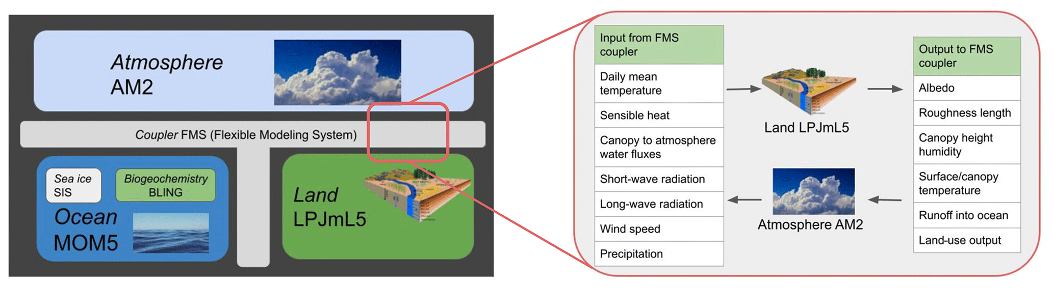
Figure 1Schematic overview of CM2Mc-LPJmL and the most important variables exchanged between LPJmL5, FMS and AM2.
2.3 Adapting LPJmL5 to implement it into the FMS coupling framework
While Sect. 2.2 described the standard LPJmL5 model as previously published, we now introduce our adaptations to LPJmL5 in order for it to be coupled with the FMS coupling framework. An overview of our coupling approach between LPJmL5 and the CM2Mc model is provided in Fig. 1. The FMS coupling software (and hence the atmosphere model) expects a certain set of variables for full dynamic coupling. We consider canopy humidity, soil and canopy temperature, roughness length and albedo as essential variables to allow dynamic vegetation to fully interact with the atmosphere, and we describe their implementation in the following. All of these variables are exchanged with the atmosphere on the so-called “fast time step”, which we currently set as 1 h. Because the offline version of LPJmL5 simulates carbon and water fluxes only at a daily time step, we introduced a sub-daily time step of the same duration as the fast time step and ensured a diurnal cycle for temperature and humidity, which is important to stabilize the atmosphere and the coupled model system (Randall et al., 1991; Kim et al., 2019). These processes included calculations of the water and energy cycles (i.e., surface temperature, evapotranspiration and water stress). Albedo and roughness lengths are expected to be less dynamic and are, thus, independent of the diurnal cycle. Hence, they are calculated at the original daily time step within LPJmL5 but are still exchanged every hour. For ecosystems that are temporarily covered by snow, sublimation is implemented by building on the simple snow model in LPJmL5, which also operates at the fast time step. On every fast time step, the coupling variables are sent from LPJmL5 to the FMS coupler. The coupler then provides the synoptic climate variables (temperature, precipitation, radiation) as the input for LPJmL5 at the next (fast) time step.
In this section, we describe our coupling approach at the interface between the land model (LPJmL5) and the FMS coupler. FMS calculates the fluxes between the different model components and provides this information to the subcomponents. The tasks of the coupler also include the calculation of air stability and surface drag; hence, it has some functionality of a land-surface model. Because it is beyond the scope of this paper to explain the processes within FMS in detail, we refer to Milly and Shmakin (2002) and Anderson et al. (2004) for further details.
2.3.1 Interface between FMS and LPJmL5
The C main function of LPJmL5 used in the offline version is replaced by a coupler function providing the interface between the internal C functions of LPJmL5 and the Fortran functions of the CM2Mc model. The coupler function is called by FMS at an hourly time step, and it calls the specific update functions of LPJmL5 at the end of each hour, day, month or year, respectively. Ingoing and outgoing data are transferred as array arguments of this function. The mapping of the coarse resolution of the CM2Mc model to the 0.5∘ × 0.5∘ resolution of LPJmL5 is done by the FMS coupler. We found that the FMS land model component must be run at LPJmL5 resolution, which is 0.5∘, so that all model components and the FMS coupler agree on which cells belong to land and which to the ocean. This yields slight changes of the land–sea mask from the original CM2M_coarse_BLING setup.
CM2Mc as well as LPJmL5 can use the message passing interface (MPI) to run the simulation in parallel on a compute cluster. CM2Mc uses FMS to set up a two-dimensional domain decomposition (i.e., it splits the global grid into rectangular domains which are mapped to concurrent MPI tasks). In contrast, the LPJmL5 grid is represented by an unsorted one-dimensional array of land cells, which is evenly distributed onto the MPI tasks. As this LPJmL5 grid is not compatible with the FMS grid exchange framework, a small wrapper library was developed for the data exchange between LPJmL5 and FMS domains. The wrapper library is called for the ingoing and outgoing data, and the time overhead for this data exchange is negligible. The coupler function as well as the wrapper library are part of the LPJmL5 distribution.
2.3.2 New canopy module
The stand-alone version of LPJmL5 does not calculate the essential coupling variables, canopy temperature and humidity, which is remedied in the coupled configuration via the addition of a new canopy module. In this new module, the canopy humidity and canopy temperature and some further quantities linked to those variables are calculated (Fig. 2). In this setting, the canopy layer corresponds to the lower boundary for the temperature in the atmosphere. The atmospheric diurnal cycle as well as the seasonal changes depend on the surface energy balance. The canopy humidity, on the other hand, is the lower boundary for the atmospheric humidity and, hence, sets the moisture content and the amount of precipitation in the atmosphere as well as the potential for evapotranspiration at the surface. A schematic overview of the different calculation steps is provided in Fig. 3.
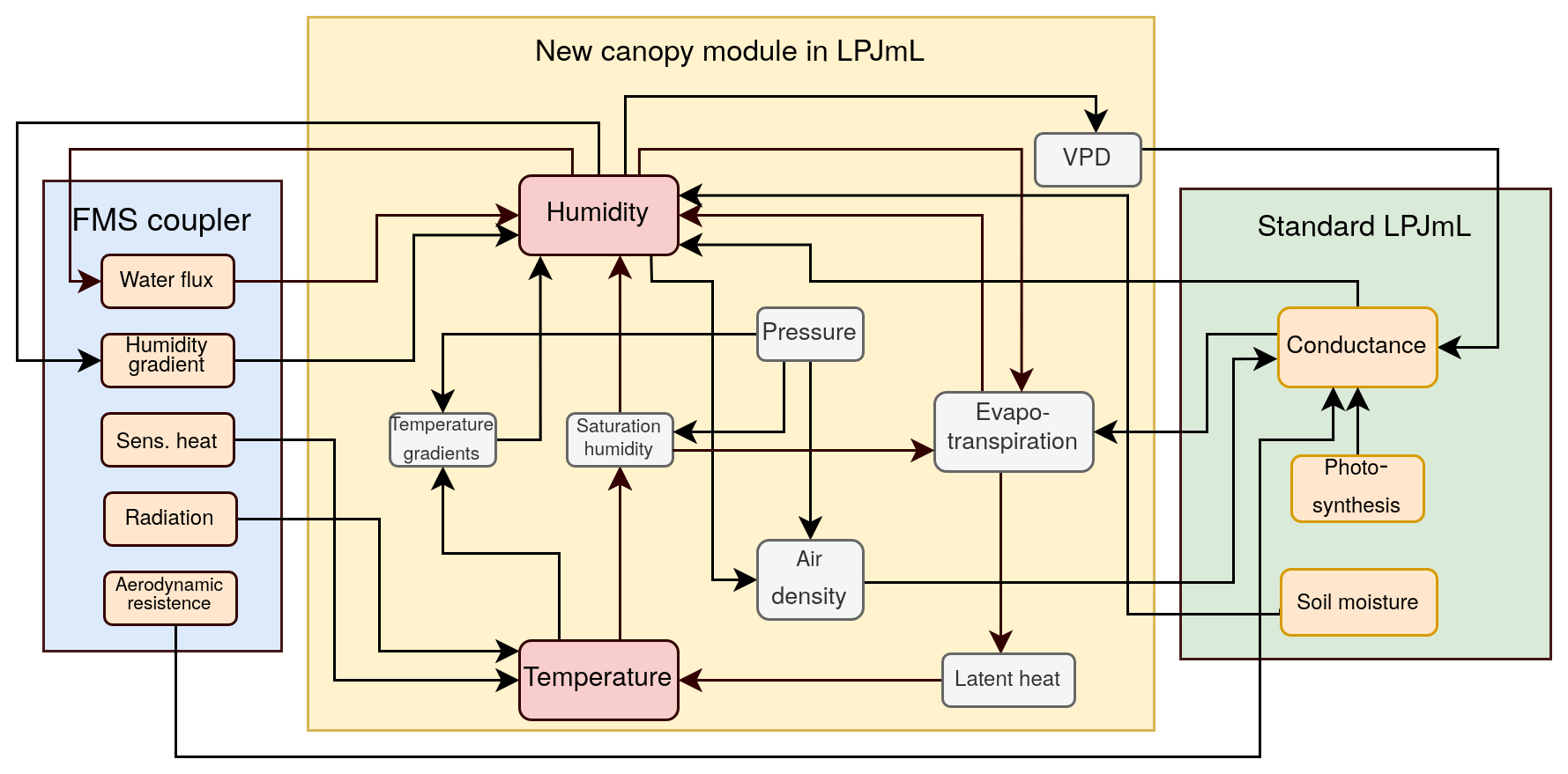
In the stand-alone version of LPJmL5, climatic input is prescribed; therefore, calculations of processes and fluxes, such as evapotranspiration, do not feed back to the atmosphere. In the coupled version, however, a small perturbation in a positive feedback loop can influence the climate and push the process towards an even larger perturbation. Thus, special attention has to be given to ensure the stability of the model by either ignoring the feedback and implementing a simple, empirical and stabilizing relationship or by increasing the complexity of the implementation, in order to get a more realistic representation of the vegetation embedded in the Earth system. The latter was done in CM2Mc-LPJmL by replacing the former simple Priestley–Taylor approach for calculating potential evapotranspiration ET0 with the more complex and process-based Penman–Monteith evapotranspiration (Monteith, 1965). The Penman–Monteith approximation also accounts for additional parameters, such as humidity, that were previously not available in the stand-alone LPJmL5 model (Fig. 2):
where Lv is the volumetric latent heat of vaporization of 2453 MJ m−3, ET0 is the evapotranspiration (in m d−1), is the slope of the vapor pressure curve (in kPa ∘C−1), Rn is the net radiation at the surface (in MJ m−2 d−1), G is the soil heat-flux density (in MJ m−2 d−1), 86 400 is the conversion factor from seconds to daily values, ρa is the air density (in kg m−3), Cp is the specific heat of dry air ( MJ kg−1 ∘C−1), is the saturated water vapor pressure (in kPa), ea is the actual water vapor pressure (in kPa), τaν is the bulk surface aerodynamic resistance for water vapor (in s m−1) and τs is the canopy surface resistance (in s m−1). γ is the psychrometric constant (in kPa ∘C−1) and is calculated as follows:
where P is the atmospheric pressure at the surface (in kPa), λ is the latent heat of vaporization of 2.45 MJ kg−1 and μ is the ratio of molecular weight of water vapor to dry air (which is 0.622). ET0 is presented here in the general daily form but is applied to the model on the sub-daily timescale; thus, it is divided by the number of time steps per day (in the current version 24).
Equation (1) uses the canopy surface resistance τs, which is the reciprocal of the non-water-stressed canopy conductance gp (in mm s−1). gp was also slightly changed, compared with Schaphoff et al. (2018b), in order to include climate feedbacks. Following Medlyn et al. (2011), we included a PFT-specific stomatal conductance parameter g1 (as defined in De Kauwe et al., 2015) and the vapor pressure deficit (D).
where g0 (in mm s−1) is a PFT-specific minimum canopy conductance scaled by FPC, occurring due to processes other than photosynthesis. pa is the ambient partial pressure of CO2 (in Pa), Adt denotes the daily net daytime photosynthesis and 1000 is the unit conversion factor from millimeters to meters. D (in Pa) can be obtained by the canopy humidity qca and the saturation humidity qsat:
While the new potential evapotranspiration is calculated at the sub-daily time step, the non-water-stressed canopy conductance is calculated at a daily time step, due to the daily calculation of the photosynthesis in LPJmL5. As climate data from FMS are available on a sub-daily basis, the photosynthesis routine uses a diurnal average of air temperature and photosynthetic active radiation.
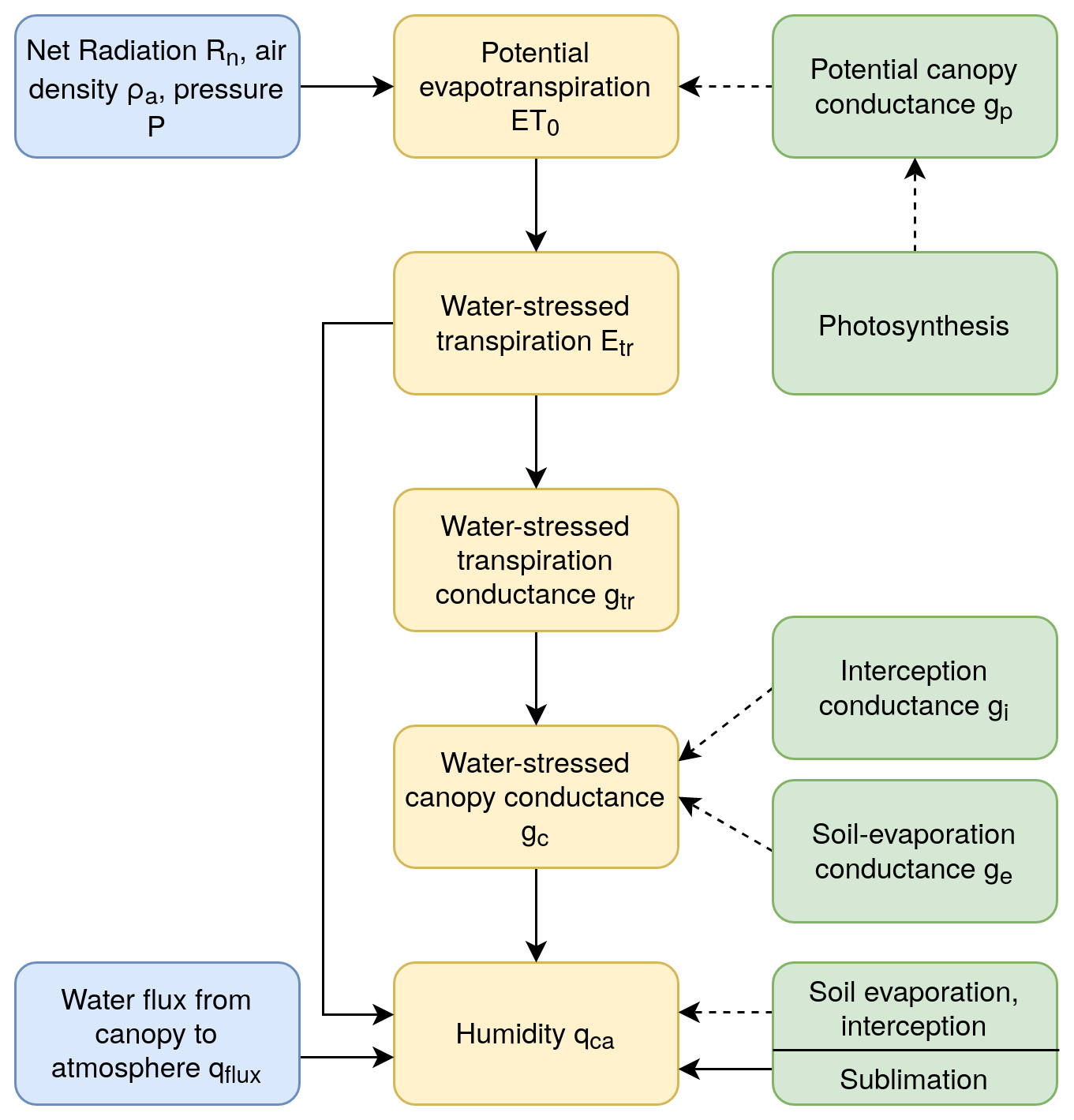
Figure 3Schematic overview of the most important processes to determine the canopy humidity. Yellow denotes newly implemented processes in the new canopy layer in LPJmL5, green denotes internal LPJmL5 calculations and blue denotes input, provided by the FMS coupler. Daily processes are indicated by a dotted line, and processes operating at a sub-daily time step are shown using a solid line.
The newly calculated potential evapotranspiration, accounting for gp, is then also used in several LPJmL5 routines (e.g., bare soil evaporation or interception) instead of the equilibrium evapotranspiration (Eq), which was based on the Priestley–Taylor formula (Schaphoff et al., 2018b).
As a next step, we calculate the water-stressed transpiration Etr, using the supply–demand functions of LPJmL5 as follows: the demand is calculated by the newly implemented potential evapotranspiration (Eq. 1, corrected by the fraction used for interception), and the supply is driven by vertical root distribution and phenology (as in Schaphoff et al., 2018b). The initial transpiration is then a function of the minimum of supply and demand for water. Following this, transpiration is subtracted from the various soil layers, depending on water availability. If the available water is not sufficient, transpiration decreases. The adjusted transpiration is consequently used in an inverse version of the Penman–Monteith formula in order to calculate the actual canopy conductance, linked to transpiration gtr.
The total canopy conductance is additionally influenced by the conductance of soil evaporation (ge) and plant interception (gi). Therefore, we use a simple approach taking the maximum rainfall interception conductance (GIMAX=10 mm s−1) into account and considering the fraction of rainfall i stored in the canopy of a biome-dependent rainfall regime (Gerten et al., 2004):
where fv is the vegetated grid cell fraction, and Pr is the daily precipitation. Pr and ET0 are applied in millimeters per second (mm s−1) here. The soil-evaporation conductance is calculated for the non-vegetated area of a grid cell and depends on the maximum soil conductance (GEMAX=10 mm s−1; Huntingford and Monteith, 1998) and an empirical scaling factor for the dependency of soil-evaporation conductance on soil water status (α0=10, Zhou et al., 2006):
where wevap is the soil water content relative to the water-holding capacity available for evaporation defined for a certain soil depth (Schaphoff et al., 2018b). Both conductances are calculated at a daily time step.
We then calculate the total canopy conductance gc by adding gtr, gi and ge and using τaν following Milly and Shmakin (2002).
where βph is the water available for photosynthesis:
with Wr as the actual soil water and as the maximum available soil water. The increment of the canopy humidity qca per time step is then calculated as follows, using gc:
where qflux is the water flux from the canopy layer to the atmosphere, provided by the FMS coupler; is the gradient of the surface temperature over time; and ET is the final evapotranspiration, consisting of transpiration, evaporation, interception and sublimation from surface or vegetation into the canopy layer. For the calculation of ET, we used the Penman–Monteith equation (Eq. 1), now applying the total water-stressed canopy conductance gc (Eq. 7). is the evaporation–humidity gradient. The total canopy conductance and the final increment of the canopy humidity, which is important for the FMS coupler, are calculated at a sub-daily time step. Equation (9) is based on Milly and Shmakin (2002) and is derived in Appendix C.
It was also necessary to implement the calculation of surface/canopy temperature within LPJmL5, which required major adaptions to the energy cycle in LPJmL5. The stand-alone LPJmL5 model calculates the temperature of different soil layers by employing a temperature transport scheme and considering air temperature as climatic input. In CM2Mc, however, the energy balance is calculated on the surface and then passed to the coupler and the atmosphere. Therefore, we had to implement this energy balance analogously in the coupled version of LPJmL5. While this surface temperature depends on several inputs from the coupler, such as radiation, it also uses several variables connected to the water cycle in LPJmL5 (evaporation, sublimation and melted water). As our approach does not account for a height-dependent canopy temperature, we used the surface temperature as an approximation for the canopy temperature, which is needed to calculate canopy humidity and evapotranspiration. Hence, surface temperature and canopy temperature are assumed to be the same, following the approach in the LaD model (Milly and Shmakin, 2002).
The soil temperature is still important for internal processes in LPJmL, such as permafrost, but it is not needed in the coupler to calculate fluxes from the land to the atmosphere. The calculation of heat transfer in the soil layers uses the heat-convection scheme as in stand-alone LPJmL5 model (Schaphoff et al., 2018b) by taking the air temperature into account, which highly depends on the canopy temperature. Both temperature calculations, for the surface/canopy temperature and for the soil temperature, operate at the fast time step.
In order to calculate the surface/canopy temperature within LPJmL5, we employed a simple energy balance formulation for the incremental change in temperature ΔT for each time step (adapted from Milly and Shmakin, 2002):
where m is the melted ice transformed to water (in kg m−2 s−1), LEf is the latent heat of the conversion of ice into water (in J kg−1), LEv is the latent heat of the conversion of water into vapor (in J kg−1), Qsn is the energy released by snow (in W m−2), H is the sensible heat provided by the FMS (in W m−2), Cs is the heat capacity of the soil (in J kg−1) and Δt is the fast time step duration (in s). Rn is used here in watts per square meter (W m−2). While the temperature is calculated individually for each stand, a weighted average over all stands within one grid cell is used in the humidity calculation and passed to the coupler. The heat balance of snow is calculated as performed for the soil layers (see Schaphoff et al., 2018b), where snow temperature changes (ΔTsnow) depend on the thermal conductivity (λsnow=0.2 W m−2 K−1) and heat capacity (Csnow=630 000 J m−3 K−1) of snow as follows:
The heat flux from snow (Qsnow) is calculated as follows:
where zsnow is the snow depth, Tair is the air temperature and is the soil temperature of the first layer.
2.3.3 Albedo and roughness length
Albedo (β), the average reflectivity of the grid cell, is calculated as in Schaphoff et al. (2018b), based on a first implementation by Strengers et al. (2010) and later improved by considering several drivers of phenology by Forkel et al. (2014):
where the albedo for bare soil βsoil is defined as 0.3, and the albedo for snow βsnow is defined as 0.7. βPFT is calculated for each PFT depending on the foliage projective cover (FPC) and the stem, litter and leaf albedo of the respective PFT. The value for each parameter is as in Schaphoff et al. (2018b). Fsnow and Fbare are the snow coverage and the fraction of bare soil, respectively. Water bodies such as lakes and rivers have a constant albedo value of 0.1.
Roughness length z0 m is calculated according to Strengers et al. (2010):
and
where zb is the height of the boundary layer under stable conditions, set to 100 m (Ronda et al., 2003); is the PFT-specific roughness length; and FPCi is the foliage projective cover of each PFT, respectively. The coupler uses the roughness length to calculate aerodynamic resistance and surface drag and provides these variables to the different sub-models of the ESM.
2.3.4 Further changes in the coupled LPJmL5
For a global model we also need to consider Antarctica, which has not been part of the standard grid of the stand-alone LPJmL5 modeling configuration. It was implemented using a simplified approach and will be replaced with the Parallel Ice Sheet Model (PISM, Winkelmann et al., 2011) in the future. For now, Antarctica is assigned the ice soil type and a constant albedo of 0.7. The temperature balance is calculated as on the other continents.
In the stand-alone LPJmL5 model, sublimation is subsumed by a constant global value of 0.1 mm d−1, likely underestimating the sublimation at high latitudes. Especially in wintertime, we do not expect much evapotranspiration; hence, the sublimation changes with meteorological conditions and becomes an important process. For this reason, we implemented the calculation of sublimation Es using the formula from Gelfan et al. (2004):
where u is the wind speed (in m s−1) from the coupler, es is the saturated vapor pressure (in mbar) and ea is the air vapor pressure (in mbar).
Furthermore, the first test runs of the coupled models proved the need to tune some LPJmL5 PFT-specific parameters: we increased the effective rooting depths of the tropical tree PFTs to 2.3 m in order to counter a negative AM2 precipitation bias in northern South America. Therefore, we increased the β value of each tropical tree PFT, describing their vertical fine-root distribution in the soil column from 0.96 as in Schaphoff et al. (2018b) to 0.99 in this study.
2.4 Model setup and forcing
In the stand-alone version, as well as in the coupled version, LPJmL5 is forced with gridded soil texture data (Nachtergaele et al., 2009). Global atmospheric CO2 values are from Mauna Loa station data (Le Quéré et al., 2015) and land-use information is from Fader et al. (2010). The SPITFIRE fire module (Thonicke et al., 2010) requires human population density as input, which is taken from Goldewijk et al. (2011), as well as lightning flashes, which are taken from the Optical Transient Detector (OTD) and Lightning Imaging Sensor (LIS) satellite product (Christian et al., 2003). In the coupled LPJmL5 version, we activated permafrost, the new phenology and SPITFIRE using the vapor pressure deficit as the fire danger index (Drüke et al., 2019). The nitrogen cycle, which is part of LPJmL5 (Von Bloh et al., 2018), was deactivated in this study. Running in the coupled model, LPJmL5 receives climatic input as, for instance, temperature, precipitation and radiation from the coupler interactively.
For the stand-alone LPJmL5 spin-up, we used the climate data (temperature and precipitation) from the Land Data Assimilation System (GLDAS; Rodell et al., 2004). The original data have a spatial resolution of 0.25∘ × 0.25∘ and a time step of 3 h. We regridded the data set to the 0.5∘ × 0.5∘ LPJmL5 resolution and aggregated it to a daily time step. For the spin-up, we recycled data from the years 1948–1978 (the earliest years available in GLDAS). Short-wave and long-wave radiation was used from the coupled model CM2Mc, where the vegetation has been calculated by LaD (Milly and Shmakin, 2002).
For the fully coupled model run, we used 20 CPUs for the land and atmosphere calculations and 8 CPUs for the ocean, totaling 28 CPUs. With these settings, 1 model year needs roughly 30 min on the PIK HPC cluster (Xeon E5-2667v3 8C 3.2 GHz, Infiniband FDR14). The number of MPI tasks is limited by the coarse resolution of the atmosphere grid. Parts of the atmosphere code can employ hybrid MPI and OpenMP parallelism, but computational costs for LPJmL5 remain unaffected.
2.5 Modeling protocol
Soil carbon and vegetation biomass need timescales of hundreds to several thousand years to reach an equilibrium with climate, which would require extremely long spin-up simulations in the coupled model. Hence, we first produce a spin-up for 5000 years with the more computationally efficient stand-alone LPJmL5 model, using climate input from GLDAS and an earlier CM2Mc-LaD run. To bring vegetation, soil and climate into a consistent equilibrium (stand-alone LPJmL5 spin-up and the restart files from CM2Mc using LaD), we subsequently perform a fully coupled run of 500 simulation years under preindustrial conditions with land use deactivated. The climate of this run is then used as forcing for another stand-alone LPJmL5 spin-up run of 5000 years, producing restart conditions much closer to the state of the coupled model. This multistep spin-up approach minimizes the time for the computationally expensive coupled model to reach a stable state.
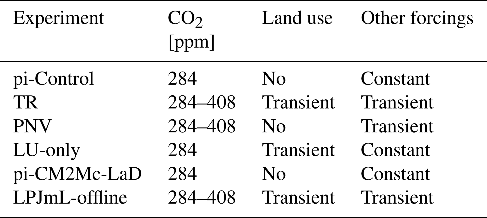
To account for changed dynamics in the coupled system, the LPJmL5 spin-up is then followed by a coupled spin-up, which runs for 500 years under preindustrial and potential natural vegetation (PNV, i.e., without land use) conditions in a fully coupled setting. This fully coupled spin-up is the starting point for the production runs (see Table 1), except for the pi-CM2Mc-LaD and LPJmL-offline experiments.
As a baseline run, we complete another 250 simulation years under preindustrial PNV conditions in addition to the 500 simulation years of the coupled spin-up, resulting in 750 simulation years with the same settings (pi-Control experiment).
The transient run (TR) with variable land use and forcings is performed for the years 1700 until 2018, using historical land-use data from 1700 onward, prescribed as outlined in Fader et al. (2010); the concentration of greenhouse gases, solar radiation, ozone concentrations and the amount of aerosols in the atmosphere are kept constant at preindustrial conditions until 1860 and then vary according to historical data. From 2004 onward, solar radiation, ozone and aerosols are kept constant due to missing data.
Similar to the TR experiment, we conduct two more experiments in order to investigate the impact of climate and land-use change in CM2Mc-LPJmL separately. Both runs are performed for the years 1700–2018: one with transient, historical climate but PNV conditions without land use (PNV experiment), and the other with transient land use but preindustrial climate (LU-only experiment).
Two additional simulation experiments are conducted that did not use the 500-year coupled spin-up: to compare the performance of CM2Mc-LPJmL against the original CM2Mc model under preindustrial conditions, we conduct a 200-year run of the CM2Mc model using the original LaD land model (pi-CM2Mc-LaD) and compare it against pi-Control. Here, we use restart files provided with the CM2Mc modeling suite. We also perform a transient stand-alone LPJmL5 (LPJmL-offline) run with a deactivated nitrogen cycle (Schaphoff et al., 2018b; Von Bloh et al., 2018) in order to compare the results to CM2Mc-LPJmL.
Table 1Overview of the simulation experiments conducted in this study. All runs, except for pi-CM2Mc-LaD and LPJmL-offline, are performed with CM2Mc-LPJmL. Other forcings include aerosols, non-CO2 greenhouse gases, ozone and the solar constant. In the case of non-transient simulations, these are kept constant at their values from the year 1860. Land use can either be transient (i.e., capturing historical changes) or be deactivated.
2.6 Model evaluation
Model performance is evaluated in terms of stability and historical climate changes, and the results are compared to pi-CM2Mc-LaD runs, LPJmL5 stand-alone and observational data. Specifically, our simulation experiments (see Table 1) are evaluated as follows: to analyze the stability of CM2Mc-LPJmL, we evaluate temperature and precipitation of the 500-year coupled spin-up run combined with the 250-year pi-Control run (750 years in total).
Climate biases in precipitation and temperature are evaluated by comparing the TR experiment from 1994 to 2003 with global evaluation data sets from ERA5 (Dee et al., 2011). During the years 1994–2003, all forcing in CM2Mc-LPJmL is transient. Simulated biomass is evaluated by comparing aboveground biomass from the TR experiment with the GlobBiomass gridded data set by Santoro (2018) and Santoro et al. (2020). GlobBiomass provides vegetation carbon for roughly the year 2010; hence, we compare it to average model data from 2006 to 2015. The PFT distribution, a measure of vegetation cover, is evaluated using data from Li et al. (2018) and Forkel et al. (2019) and comparing these data with results from the TR experiment for the years 2006–2015.
The historical temperature increase is quantified by comparing the transient temperature increase between 1860 and 2018 of the TR experiment with GISTEMP data (Lenssen et al., 2019). GISTEMP combines various measurements from meteorological stations. To evaluate the impact of changes in atmospheric forcing on the spatial distribution of climate parameters and vegetation, results from the last 10 years of the pi-Control experiment are compared with results from 2006 to 2015 of the PNV experiment (Sect. S2). For analyzing land-use sensitivity (without variability in the atmospheric forcing), we compare the last 10 years of the pi-Control and the years 2006–2015 of the LU-only experiment against each other.
In the Supplement, we further provide a comparison of the results of CM2Mc-LPJmL and CM2Mc-LaD, using an average over the last 10 years of the pi-Control and the pi-CM2Mc-LaD experiments (Sect. S3), as well as a comparison with Coupled Model Intercomparison Project Phase 5 (CMIP5) data (Taylor et al., 2012) and LPJmL5-offline (Sect. S4).
As evaluation metrics, we used the normalized mean error (NME; Kelley et al., 2013):
where yi is the simulated value in grid cell i, and xi is the observed value in grid cell i. is the mean observed value. The NME is one if the model is as good as using the data mean as a predictor, larger than one for worse performance and zero for perfect agreement. We use this metric for the evaluation of the performance of temperature, precipitation and aboveground biomass.
The evaluation of the model performance is provided in Sect. 3.1, and the impact of land-use change on the results of the coupled CM2Mc-LPJmL model is analyzed in Sect. 3.2.
3.1 Model performance
Here, we evaluate the performance of CM2Mc-LPJmL against climate and biosphere observations by first looking into the long-term stability of global mean surface temperature (referred to as temperature, hereafter) and precipitation (Sect. 3.1.1) from the pi-Control experiment, before evaluating the historical temperature increase of the coupled model, using the TR experiment results. Finally, a detailed analysis of climate (Sect. 3.1.2 and 3.1.3) and vegetation cover (Sect. 3.1.4) is provided, also based on the TR experiment.
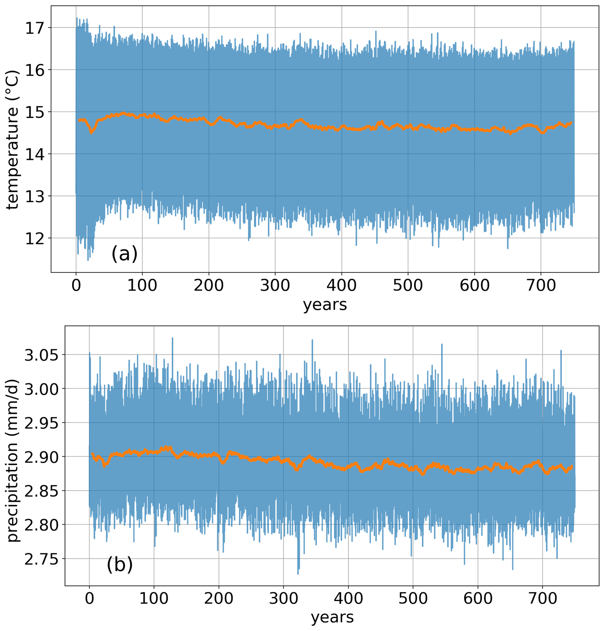
Figure 4Time series of monthly mean global (a) temperature and (b) precipitation (blue lines), and the corresponding 10-year running means (orange lines) in the pi-Control experiment.
3.1.1 Model stability
The analysis of the model stability was based on the pi-Control experiment, which ran over 750 years in total (see Sect. 2.5 for details). Here, we evaluate temperature and precipitation in terms of absolute values as well as the rate of change over time and the variability.
After the initial 300 years, the global temperature remains relatively stable at ca. 14.7 ∘C over the remaining simulation period of 400 years with a slight drift of less than of 0.05 ∘C per 100 years (Fig. 4a). The interannual variability in this period is ca. 0.1–0.2 ∘C. The decreasing temperature over most of the 750-year simulation period can be explained by the energy uptake of the ocean, as deep ocean layers are not yet in equilibrium. The average precipitation follows a similar trend as temperature and reaches a relatively stable state at around 2.88 mm d−1 after ca. 400 years, changing less than 0.01 mm d−1 over the remaining period (Fig. 4b). The interannual variability is 0.01–0.02 mm d−1.
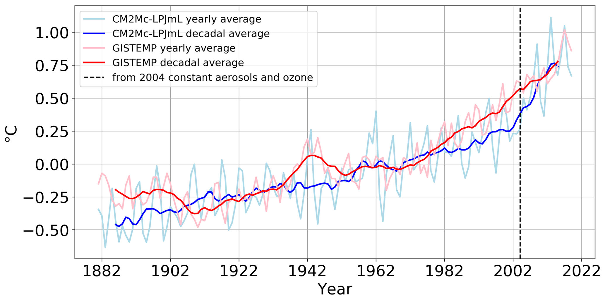
Figure 5Yearly and decadal global mean temperature anomaly (relative to the 1951–1980 reference period) of the TR experiment of CM2Mc-LPJmL compared to GISTEMP data from 1880 to 2018. Note that, from 2004 on, only greenhouse gas forcing remains, while aerosols, solar radiation and ozone are set to their corresponding 2003 values.
3.1.2 Temperature evolution over the historical period
The temperature evolution over the historical period (and hence the climate sensitivity to changes in atmospheric forcing) is evaluated by comparing the transient temperature increase in the 1880–2018 period of the TR experiment to GISTEMP evaluation data (Lenssen et al., 2019). We further evaluate the spatial impact of historical climate change without land use by comparing the years 2006–2015 of the PNV experiment with the last 10 years of the pi-Control experiment in the Supplement (Sect. S2).
The temperature evolution over the historical period from 1880 to 2018 is well captured as compared to GISTEMP evaluation data (Fig. 5). Throughout the displayed period, temperature anomalies are negative before the year 1962 and remain positive afterwards, as climate change is accelerating. While the temperature anomalies are slightly underestimated between 1980 and 2010, GISTEMP and the TR experiment both have an average global temperature increase of 0.75 ∘C in the year 2018 relative to the reference period from 1951 to 1980. Our results are also within the range of CMIP5 models (Kattsov et al., 2013; Taylor et al., 2012, Sect. S4). The interannual variability in CM2Mc-LPJmL is ca. 0.5 ∘C and, thus, larger than in the GISTEMP data (ca. 0.25 ∘C), although the decadal changes are smaller in CM2Mc-LPJmL.
In the PNV experiment, climate change is also well captured, but it is weaker than when land use is included in the model (Fig. S5).
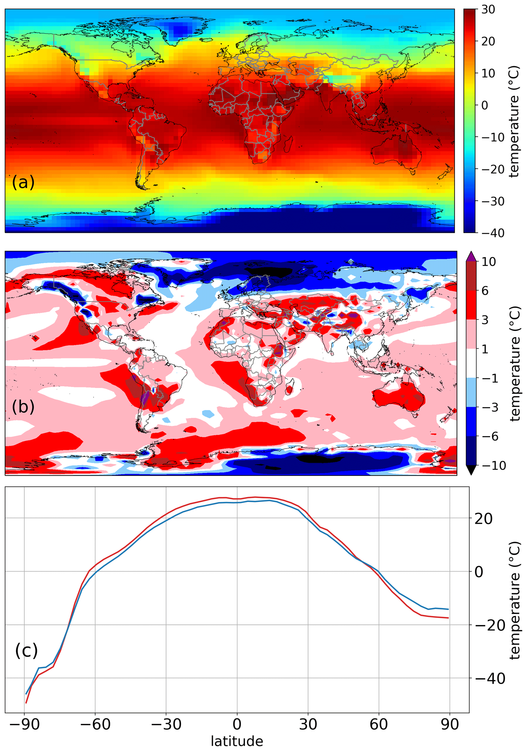
Figure 6(a) Global mean surface temperature of the TR experiment over the 1994–2003 period. (b) Surface temperature anomalies between CM2Mc-LPJmL (TR) and ERA5 data over the 1994–2003 period. (c) Latitudinal temperature mean of TR (red line) and ERA5 data (blue line) for the 1994–2003 period.
3.1.3 Surface temperature evaluation
Basic climate patterns are well captured in the annual mean surface temperature (Fig. 6a), as temperatures are increasing from polar temperatures of below −10 ∘C towards the Equator with a maximum of ca. 25–30 ∘C in the tropics. Desert regions are usually warmer, whereas mountainous regions are colder than the surrounding area. In the high latitudes, ocean cells are usually a bit warmer than land cells due to the ocean's ability to store heat.
Between 1994 and 2003, the average global temperature is 15.6 ∘C compared with 14.3 ∘C in the ERA5 data set with a NME of 0.16. While the temperatures in the tropics and temperate zone are slightly overestimated (by ca. 1 ∘C), the poles and the boreal zone show a large negative temperature bias (up to −10 ∘C) (Fig. 6b). The Southern Ocean has a significant positive temperature bias (ca. 3 ∘C on average). Large differences between CM2Mc-LPJmL and ERA5 are also visible for mountainous areas, where the temperature bias is partly due to the coarse resolution of the model not adequately capturing the orographic influence of most mountain ranges on climate (e.g., the Andes or Himalaya).
While the seasonal cycle is usually well captured in CM2Mc-LPJmL, especially in Antarctica a strong seasonal temperature bias is partly balanced out in the annual mean temperature. The temperature over Antarctica is largely overestimated during the Southern Hemisphere summer, whereas it is underestimated during the Southern Hemisphere winter (Figs. S1, S2).
The latitudinal distribution of modeled mean temperature between 1994 and 2003 (Fig. 6c) shows similar values to ERA5 data from high- to midlatitudes in the Northern Hemisphere, but a slight overestimation in parts of the temperate zone and the tropics (between 70∘ S and 40∘ N). Specifically, the cold bias in the boreal zone leads to a slight underestimation of temperature between 60 and 90∘ N.
The comparison of CM2Mc-LPJmL (pi-Control) and pi-CM2Mc-LaD (as in Galbraith et al., 2011) shows that similar biases in relation to ERA5 are present in both model versions. For example, both model versions slightly overestimate global temperature (Fig. S6). The strong regional biases compared with ERA5 data are also present in both model setups (Fig. S6) and are, therefore, not due to the implementation of LPJmL5.
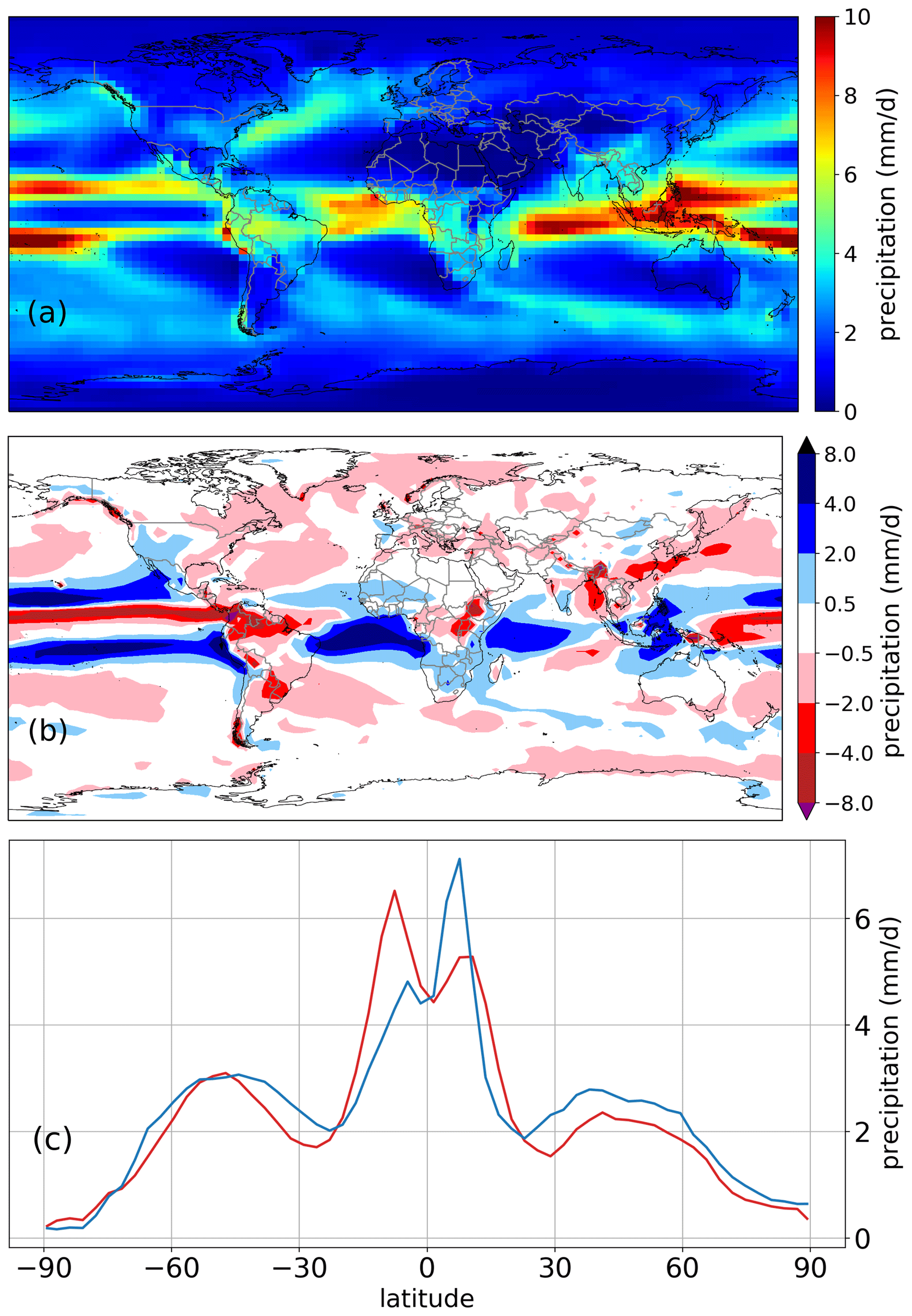
Figure 7(a) Global mean precipitation of the TR experiment for the 1994–2003 period. (b) Precipitation anomalies between CM2Mc-LPJmL (TR) and ERA5 data over the 1994–2003 period. (c) Latitudinal temperature mean of TR (red line) and ERA5 data (blue line) over the 1994–2003 period.
3.1.4 Precipitation evaluation
The spatiotemporal pattern of global precipitation is well simulated with a global average of 2.86 mm d−1 and a maximum of up to 10 mm d−1 in the tropics close to the Intertropical Convergence Zone (ITCZ; Fig. 7a). Regions with little to no vegetation, such as deserts and polar areas, receive very little precipitation throughout the year.
Precipitation biases with respect to ERA5 data are, however, stronger than temperature biases, with an NME of 0.50 compared with 0.16 for temperature (Fig. 7b). The biases are strongest at the Equator with an apparent shift of the ITCZ. While precipitation in the Pacific is underestimated directly at the Equator, it is overestimated north and south of the Equator (Fig. 7b). Moreover, northern South America shows a large negative precipitation bias.
The seasonal patterns (Figs. S3, S4) confirm the imprecise modeling of the ITCZ, which remains north and south of the Equator for a large part of the year and passes the Equator region relatively swiftly. While precipitation south of the Equator is overestimated, it is underestimated north of it.
The latitudinal annual mean precipitation between 1994 and 2003 (Fig. 7c) compares well with observations, displaying the global precipitation maximum in the tropics, local minima in the subtropics and very low values at high latitudes. The tropics, however, show a shifted maximum. While the ERA5 global precipitation maximum over the Pacific is at ca. 10∘ N and a local smaller maximum is at −10∘ S, CM2Mc-LPJmL models the global maximum at roughly −10∘ S and a smaller local maximum at ca. 10∘ N. The difference between the two maxima is less pronounced compared with ERA5.
The comparison of the results of CM2Mc-LPJmL with the original pi-CM2Mc-LaD model shows similar biases in relation to ERA5 for both model versions. Neither of the models precisely captures the behavior of the ITCZ, especially over the Pacific. Both models also show a large dry bias in northern South America (Fig. S6).

Figure 8(a) Mean global aboveground biomass of GlobBiomass evaluation data. (b) Mean global aboveground biomass of CM2Mc-LPJmL (TR) over the 2006–2015 period. (c) Difference in the aboveground biomass between CM2Mc-LPJmL and GlobBiomass evaluation data. Blue (red) denotes an overestimation (underestimation) of biomass by CM2Mc-LPJmL. (d) Latitudinal sum of aboveground biomass from CM2Mc-LPJmL (blue line, R2=0.64, NME = 0.56), stand-alone LPJmL5 (black line, R2=0.94, NME = 0.35) input data and GlobBiomass evaluation data (red line).
3.1.5 Vegetation cover and biomass
While the evaluation of temperature and precipitation is performed for the years 1994–2003, we compare average model results for aboveground biomass (AGB) and the dominant PFT for the years 2006–2015 due to availability of evaluation data.
Simulated AGB shows a good pattern overall, with the largest values in the tropics, decreasing biomass in the subtropics, and a local maximum in the temperate and boreal zone (Fig. 8d). In vegetation-free areas, such as deserts or polar regions, simulated AGB is zero or very close to zero (less than 200 g C m−2). When comparing AGB against GlobBiomass (Fig. 8a), spatial differences emerge (Fig. 8c). While simulated AGB is slightly overestimated in boreal North America and Asia, it is underestimated in the European temperate zone and in Scandinavia, extending into eastern Europe and West Siberia. In most of the other temperate, Mediterranean-type and subtropical regions, AGB matches the observed values. In the tropics, AGB is overestimated in semiarid regions, whereas wet tropical rainforests are mostly underestimated, especially the eastern Amazon. AGB shows good agreement in the seasonally dry Cerrado region in South America but appears to be overestimated in the Caatinga in northeastern Brazil. In central Australia, AGB matches observations but is overestimated in the northern part of the continent and underestimated in the southeastern part (Fig. 8c).
Figure 8d compares the latitudinal mean of CM2Mc-LPJmL and LPJmL-offline with the evaluation data. LPJmL-offline shows better performance than the coupled model, with a smaller NME (0.35 vs. 0.56) and a better R2 (0.94 vs. 0.64). While both models underestimate biomass in the tropics, biomass in the boreal zone is overestimated by CM2Mc-LPJmL and underestimated by the stand-alone LPJmL5 model compared with GlobBiomass. The LPJmL5 stand-alone version is forced by a reanalysis climatic input with a 0.5∘ spatial resolution, and the model is calibrated to this specific climate conditions; therefore, better model performance is expected. Modeled biomass is also within the range of CMIP5 models (Fig. S7).

Figure 9(a) The dominant PFT for each cell, modeled by CM2Mc-LPJmL. Cells with more than 50 % land use are masked using gray. Cells with less than 200 g C m−2 are shown using white. Full names of PFTs can be found in Appendix B. (b) The sum of squares errors of ESA CCI land cover for each PFT in each cell. Blue areas have a small error, and red areas have a large error. The error shown here is absolute; hence, areas with a low PFT cover for both model and evaluation data are small compared with areas with a large PFT cover.
The geographic distribution of dominant PFT cover in CM2Mc-LPJmL follows the spatial pattern of the biomass distribution (Fig. 9a). The tropics are mostly dominated by the evergreen tree PFT. In the tropical savanna areas, the tropical deciduous tree PFT dominates, along with the C4-grass PFT. The temperate zone is dominated by land use with some summergreen trees – most common in areas such as Europe. The boreal zone is correctly covered by boreal needle-leaved and boreal summergreen trees, and the tundra zone is covered with polar grasses. To better visualize the model error for the PFT distribution, we produced an error map that consists of the sum of the square error for each PFT per cell (Fig. 9b). In tropical rainforests, the error with respect to the evaluation data is relatively small. Drier savanna areas show a much larger error, as do parts of the temperate and the boreal zone. Areas with a small FPC fraction show a small error because the error metric takes absolute errors into account. This applies to desert regions in Africa, the Arabian Peninsula and central Australia.
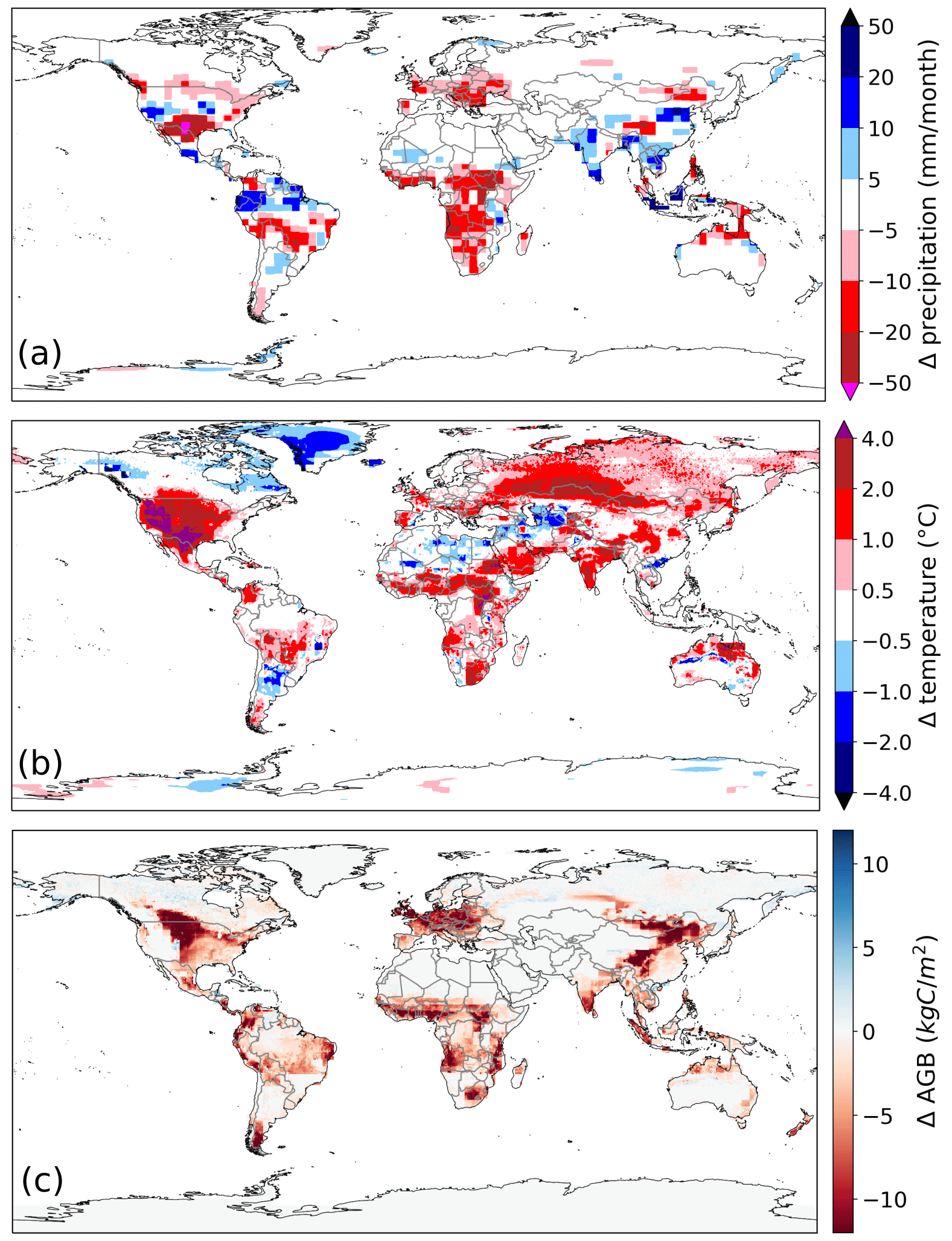
Figure 10Difference between the LU-only (2006–2015) and the pi-Control (last 10 years) experiments for (a) mean precipitation, (b) mean surface air temperature and (c) mean aboveground biomass.
3.2 Impact of land-use changes on the coupled system
In order to isolate the impact of land-use change, we kept the climate constant and allowed land use to change (LU-only, see Table 1). We compared precipitation, temperature and AGB for the years 2006–2015 of the LU-only experiment against the last 10 years of pi-Control to evaluate the absolute impact of changing land use.
Most regions with a decreasing biomass and an increasing temperature show decreasing precipitation (e.g., the Brazilian Cerrado or southern Africa). This is due to reduced evapotranspiration of agriculture and pasture compared with natural vegetation (Fig. 10a). Precipitation increases in regions where natural vegetation benefits from increased temperatures (i.e., in mountainous regions, in India and in parts of southeast Asia) (Fig. 10a).
Due to the replacement of natural vegetation with crops and managed grass, the total biomass is lower than in the pi-Control experiment in regions with large land-use areas (e.g., Europe or the USA) (Fig. 10c). As a consequence, surface temperature increases in these areas (Fig. 10b), leading to a global increase of ca. 0.5 ∘C of average land-surface air temperature. In the LU-only experiment, temperature additionally increases in regions where little to no land-use change occurred (e.g., over northern Australia and Siberia) (Fig. 10b). Over several sparsely vegetated areas, such as in the Sahara, northeastern Canada and Greenland, temperature decreases. Temperatures in tropical regions, such as in the Amazon Basin and central Africa, are unaffected, as is the temperature in most desert and polar regions. For these regions, the amount of biomass remains the same as in the pi-Control experiment (Fig. 10c).
In this study, we show the successful biophysical coupling of the whole-ecosystem DGVM LPJmL5 into the coarse-resolution version of the GFDL CM2 coupled climate model (CM2Mc), replacing the simple land-surface model of CM2Mc with LPJmL5. In order to couple the stand-alone LPJmL5 version to CM2Mc, some well-functioning model elements and structures had to be revised and modified to work in a fully coupled climate model and to meet the essential coupling variables required by the coupler and the atmosphere modules. Even though LPJmL was developed as a stand-alone DGVM, its coupling to CM2Mc does not significantly change the temperature and precipitation patterns; instead, it enables us to explore biophysical climate–vegetation feedbacks. Moreover, the resulting model is within the range of CMIP5 models as stated in Assessment Report 5 (see Fig. S7 in the Supplement and Kattsov et al., 2013).
In Sect. 4.1, we discuss the challenges of coupling LPJmL5 to CM2Mc and the evaluation of the coupled system; in Sect. 4.2, we examine the model application to simulate historical climate and land-use change; and in Sect. 4.3, we present an outlook on how the advantages of our modeling approach can be used best in future work.
4.1 Challenges of coupling LPJmL5 into CM2Mc
The results shown in Sect. 3 demonstrate that we achieved stable model performance with respect to climate–biosphere interactions after a potential natural vegetation spin-up period of 500 years. By achieving a stable climate in terms of surface temperature and precipitation, other variables in the model, such as carbon stocks of the biosphere (see Fig. S8 in the Supplement) and ocean carbon stocks, are also assumed to stabilize (although possibly on a different timescale).
The temperature and precipitation climate variables show very similar biases to CM2Mc with LaD (see Figs. 6, 7 and S6). In other words, the relatively large bias in CM2Mc in certain regions also occurs when using the prescribed and idealized vegetation cover from LaD and is, therefore, not introduced by the coupling to LPJmL. The distribution of plant functional types and aboveground biomass are well simulated in most regions (Figs. 8, 9).
The performance of the coupled LPJmL5 is directly sensitive to biases in the climate input produced by the AM2 atmosphere model. These biases can lead to a different vegetation state, which affects vegetation feedbacks to the atmosphere with possible increasing biases in AM2. This feedback loop is responsible for the deviations in our LPJmL vegetation results compared with stand-alone simulation experiments without such feedbacks to the atmosphere. In the latter case, error propagation from the climate input is avoided by forcing the model with bias-corrected climate data (Frieler et al., 2017). In our model approach, we abstained from bias or flux corrections within the coupled model to maintain more realistic feedbacks and to allow its application to future and paleoclimate conditions. Furthermore, small problems in the parameterization of important processes can lead to larger problems in the whole state of the modeled Earth system. For instance, the temperature and water cycle calculations have a strong interconnection; hence, a small error in the calculation of the water or energy cycle could lead to a runaway temperature and cause vegetation dieback for the wrong reasons. By adapting factors such as the calculation of evapotranspiration and sublimation (see Sect. 2.3.2 and 2.3.4), we managed to keep the model relatively stable.
CM2Mc, when coupled with either LaD or LPJmL5, has a positive temperature bias of 1.3 ∘C, which is within the range of published Earth system models (Kattsov et al., 2013). The temperature biases in CM2Mc are especially large in the polar and in other at least partially snow-covered regions. In the northern latitudes, a negative temperature bias led to a large vegetation mortality in areas such as Scandinavia in a previous model version (not shown). By adapting the simple snow model within LPJmL, we obtained a stable vegetation of polar grasses and boreal trees in boreal Eurasia (see Sect. 2.3.4 for methods and Fig. 9 for results). A completely revised snow model or even a parallel ice sheet model could improve the modeling performance further.
Globally, the biomass cover is captured well by CM2Mc-LPJmL (Fig. 8). However, a dry bias in northern South America led to a strong underestimation in the biomass productivity in an early version of CM2Mc-LPJmL. The modeling was improved by using the abovementioned Penman–Monteith parameterization for evapotranspiration (Sect. 2.3.2) and by increasing the tropical rooting depths and, hence, the soil water access of the trees (Sakschewski et al., 2020). Global biomass patterns are now also comparable with the stand-alone LPJmL5 version (Fig. 8d).
Additionally, the coarse resolution of AM2 contributes to the simulated climate and vegetation anomalies, which can usually be expected when running fully coupled ESMs (Galbraith et al., 2011). Although LPJmL runs in the native resolution of 0.5∘ × 0.5∘, the atmosphere and, hence, the climatic input to LPJmL has a resolution of 3∘ × 3.75∘. While this resolution is necessary for a low computational cost, it can decrease the model accuracy over regions such as mountain ranges like the Andes. The model smooths the height of the Andes to the coarse grid cell size, which leads to warmer temperatures in the high mountain areas and to a colder temperature in the low areas. Small biomes, such as the Caatinga in Brazil, have the size of a few grid cells or are even smaller than one grid cell; hence, their unique climate can not be sufficiently captured by the coarse resolution of the atmosphere model. This could be improved by using a smaller grid size, although at the expense of higher computational costs.
As LPJmL accounts for large carbon stores, such as soil carbon, a long spin-up of several thousand years is necessary to get the carbon pools into equilibrium (Schaphoff et al., 2018b). To save computation time, this spin-up has been calculated with the stand-alone LPJmL version. Due to differences in the forcing of the stand-alone LPJmL version and the fully coupled model, there is still a small offset in the beginning of the fully coupled spin-up run. After ca. 300 years, temperature and precipitation have reached a state close to an equilibrium (Fig. 4), and the model can be used for further scenarios and possible applications. Without using the multistep spin-up, as described in the methods (Sect. 2.5), the time to reach a stable state would be several times larger.
4.2 Climate and land-use change in CM2Mc-LPJmL
In addition to regional temperature patterns, the global temperature trends in historical climate and land-use change simulations are often used as another important evaluation metric, closely related to the climate sensitivity of Earth system models (Kattsov et al., 2013). Compared to GISTEMP evaluation data (Lenssen et al., 2019), the global temperature evolution over the historical period from 1860 until 2018 is well captured in CM2Mc-LPJmL (Fig. 5). The temperature increase in this period is also comparable to Kattsov et al. (2013). Therefore, the model is able to model the response of the climate system and, hence, the response of the biosphere to historical climate change.
To realistically model regional responses to climate change, the spatial temperature biases have to be taken into account. Temperature biases on land, which are sometimes up to 2 ∘C, are larger than temperature increases during historic climate change. These biases have to be considered, when interpreting results from future model runs. Furthermore, the model does not account for climate modes and extreme events (e.g., El Niño–Southern Oscillation); hence, the interannual variability is smaller than expected. The interpretability of future runs is also hampered by the uncertain effect of CO2 fertilization (Clark et al., 2013; Körner, 1993). This effect is relatively strong in LPJmL, leading to an increase in vegetation productivity at increasing CO2 and temperature. The CO2 fertilization effect under current climate has a stronger impact in LPJmL5 than heat stress in a warming climate. Activating the nitrogen cycle in LPJmL5 could reduce this strong effect by taking nitrogen limitation on vegetation productivity into account (Von Bloh et al., 2018). However, historical biomass increase resulting from the CO2 fertilization effect agrees with previous studies (e.g., Zhu et al., 2016). A decrease in biomass in the historical period occurs almost exclusively in regions with land-use expansion.
Land use and land-use management are often neglected in Earth system models, which leads to an inaccurate modeled temperature impact through land-use changes (Luyssaert et al., 2014). As only ca. 30 % of the land surface remains untouched by humans, a correct representation of land-use practices is important for modeling climate change of the 21st century (Levis, 2010). CM2Mc-LPJmL uses the advanced land-use scheme of LPJmL5, which includes various management practices (e.g., harvest and irrigation) for 12 different crop types.
By including land-use change in CM2Mc-LPJmL, natural vegetation is partially replaced by pasture and crops over time. This decreases biomass and affects the climate in three different aspects: (1) less vegetation transpires less water, which decreases the water flux to the atmosphere, cooling by latent heat, humidity and precipitation (Gkatsopoulos, 2017); (2) the albedo of crops is larger than that of closed forest, leading to a lower temperature (Unger, 2014); and (3) the roughness lengths decrease, which increases temperature (Hoffmann and Jackson, 2000). While these effects mostly consist of a cooling through larger albedo and a warming through a smaller flux of latent and sensible heat, the net effect in CM2Mc-LPJmL is a warming climate in most areas. Especially in the tropics, the latent and sensible heat fluxes outweigh a potential cooling by albedo increases. Furthermore, the biophysical effect of land-use changes is highly sensitive to changes in roughness lengths and albedo for the different PFTs and crop functional types as well as to changes in different management options, such as a different irrigation scheme (Kueppers et al., 2007).
Other studies, such as Luyssaert et al. (2014) and Alkama and Cescatti (2016), have also found a warming resulting from changes in land use and management, based on observed data. In contrast to our results, modeling studies such as Strengers et al. (2010) and Boysen et al. (2020) found a cooling in temperate and boreal regions due to the biophysical effects of land-use change. Whereas Strengers et al. (2010) used a relatively simple atmospheric model and coupling approach between the biosphere and atmosphere, Boysen et al. (2020) compared the effect of the replacement of forest with grassland for nine Earth system models. However, this methodology is different from the modeling approach in LPJmL5 where actual changes in land use and land management are captured as well as sowing, growth and harvest of 12 different crop types, and managed grassland is also explicitly simulated.
4.3 Outlook
Using the advanced land-use scheme of LPJmL5 and the capability of CM2Mc to accurately model climate change, the combined model CM2Mc-LPJmL is a powerful tool to model future trajectories of the Earth system. It allows for the calculation of various land-use change scenarios or management practices under changing climate in a computational efficient way. It is further possible to separately investigate different biophysical processes and feedbacks while forcing the model with representative concentration pathways (RCPs). Given the speed and relatively low computational cost of the model, even long-term equilibrium experiment of several hundred years can be completed within days to a few weeks.
While CM2Mc-LPJmL is fully biophysically coupled, the biogeochemical coupling is not yet included. Each sub-model accounts for a local carbon cycle and balance, but the carbon cycle is not yet closed for the whole model. For this study, we prescribed the atmospheric CO2 concentration in all model runs; therefore, a closed carbon cycle was not necessary. A fully closed carbon cycle is planned for future studies.
The key advantages of CM2Mc-LPJmL are the relatively fast and computational inexpensive atmosphere–ocean general circulation model (due to its relatively low spatial resolution) and the ability to investigate detailed feedbacks of the biosphere using the state-of-the-art DGVM LPJmL5. While LPJmL5 is constantly improved, recent new features such as a process-based nitrogen cycle (Von Bloh et al., 2018), a tillage system for land use (Lutz et al., 2019) or variable root growth (Sakschewski et al., 2020) can be integrated into the modeling framework consecutively and tested in the Earth system model. The coupled model also remains flexible for new model compartments such as a new atmosphere or a new ocean model, which are compatible with FMS. GFDL has already released the newest AM4 atmospheric model (Zhao et al., 2018) as well as MOM6, which is a state-of-the-art ocean model (Adcroft et al., 2019). Both could be integrated into the preexisting modeling framework and are expected to further reduce model bias.
In this study, we demonstrate the successful biophysical coupling of the state-of-the-art LPJmL5 DGVM into the CM2Mc coupled climate model. To do so, we replace the simple LaD static vegetation model with the LPJmL5 whole-ecosystem model. Thus, major adaptations were implemented in LPJmL5. These included the implementation of a new canopy module and a sub-daily time step in LPJmL5. The performance of the newly coupled model is similar to CM2Mc-LaD (Galbraith et al., 2011) and comparable to CMIP5 (Kattsov et al., 2013). The NME of temperature and precipitation showed good values of 0.16 and 0.50. The vegetation cover and biomass (NME of 0.56) is also well captured compared to evaluation data. Some regions, however, exhibit large temperature and precipitation biases due to the old atmosphere model and its coarse spatial resolution. Furthermore, the model shows stable performance over 750 years and reasonable reactions to climate and land-use change. The average surface temperature increases by ca. 0.75 ∘C in 2018 compared with the 1950–1980 period. Land-use expansion over the last 300 years led to a generally drier and ca. 0.5 ∘C warmer climate.
The fully coupled energy and water cycle allows for the investigation of the impact of biophysical atmosphere–biosphere feedbacks on global climate trajectories as well as the quantification of the impacts of deforestation or afforestation scenarios. CM2Mc-LPJmL might further aid in identifying tipping points and planetary boundaries, especially in the biosphere. By using LPJmL5, we can make use of functions such as its advanced land-use scheme, the sophisticated SPITFIRE process-based fire model (Thonicke et al., 2010), a representation of permafrost and state-of-the-art water cycling (Schaphoff et al., 2018b) as well as the ability to incorporate future model developments.
| Variable | Description | Unit |
| Lv | Volumetric latent heat of vaporization | MJ m−3 |
| ET0 | Potential evapotranspiration | m d−1 |
| Slope of vapor pressure curve | kPa ∘C−1 | |
| Rn | Net radiation at surface | MJ m−2 d−1 |
| G | Soil heat-flux density | MJ m−2 d−1 |
| ρa | Air density | kg m−3 |
| Cp | Specific heat of dry air | MJ kg−1 ∘C−1 |
| Saturated water vapor pressure | kPa | |
| ea | Actual water vapor pressure | kPa |
| τaν | Bulk surface aerodynamic resistance for water vapor | s m−1 |
| τs | Canopy surface resistance | s m−1 |
| λ | Latent heat of vaporization | MJ kg−1 |
| γ | Psychrometric constant | kPa ∘C−1 |
| P | Atmospheric pressure | kPa |
| μ | Ratio of molecular weight of water vapor to dry air | – |
| gp | Non-water-stressed canopy conductance | mm s−1 |
| g1 | Stomatal conductance parameter | – |
| D | Vapor pressure deficit | Pa |
| g0 | Minimum canopy conductance | mm s−1 |
| pa | Ambient partial pressure of CO2 | Pa |
| qsat | Saturation humidity | Pa |
| qca | Canopy humidity | Pa |
| Adt | Daily net daytime photosynthesis | – |
| Eq | Equilibrium evapotranspiration | mm s−1 |
| gtr | Canopy conductance for transpiration | mm s−1 |
| ge | Canopy conductance for soil evaporation | mm s−1 |
| gi | Canopy conductance for interception | mm s−1 |
| GImax | Maximum rainfall interception | mm s−1 |
| i | Fraction of rainfall stored in the canopy | – |
| fv | Vegetated grid cell fraction | – |
| Pr | Daily precipitation | mm d−1 |
| GEmax | Maximum soil-evaporation conductance | mm s−1 |
| wevap | Relative soil water content | – |
| α0 | Empirical scaling factor for soil conductance | – |
| Wr | Actual soil water | L m−3 |
| Maximum available soil water | L m−3 | |
| βph | Water available for photosynthesis | – |
| ET | Water-stressed evapotranspiration | mm s−1 |
| gc | Total canopy conductance | mm s−1 |
| T | Temperature | ∘C |
| qflux | Water flux from the canopy layer to the atmosphere | mm s−1 |
| m | Melted ice transformed to water | kg m−2 s−1 |
| LEf | Latent heat of the phase transition of ice into water | J kg−1 |
| LEv | Latent heat of the phase transition of ice into vapor | J kg−1 |
| Qsn | Energy released by snow | W m−2 |
| H | Sensible heat | W m−2 |
| Cs | Heat capacity of the soil | J kg−1 |
| Δt | Fast time step | s |
| λsnow | Thermal conductivity | W m−2 K−1 |
| Csnow | Heat capacity of snow | J m−3 K−1 |
| Variable | Description | Unit |
| zsnow | Snow depth | m |
| Qsnow | Heat flux from snow | W m−2 |
| β | Surface albedo | – |
| Fbare | Snow coverage | – |
| Fbare | Fraction of bare soil | – |
| z0 m | Roughness length | m |
| zb | Height of boundary layer under stable conditions | m |
| PFT-specific roughness length | m | |
| Es | Sublimation | mm s−1 |
| u | Wind speed | m s−1 |
| TrBE | Tropical broad-leaved evergreen tree |
| TrBR | Tropical broad-leaved raingreen tree |
| TeNE | Temperate needle-leaved evergreen tree |
| TeBE | Temperate broad-leaved evergreen tree |
| TeBS | Temperate broad-leaved summergreen tree |
| BoNE | Boreal needle-leaved evergreen tree |
| BoBS | Boreal broad-leaved summergreen tree |
| BoNS | Boreal needle-leaved summergreen tree |
| TrH | Tropical herbaceous |
| TeH | Temperate herbaceous |
| PoH | Polar herbaceous |
Assuming equilibrium conditions, the flux entering the canopy layer from soil and vegetation through evapotranspiration ET or Ein equals the flux leaving the canopy layer into the atmosphere qflux or Eout.
The water fluxes for the next time step t+1 yield
using
Using Milly and Shmakin (2002) and Eq. (7) from this paper yields the following for E:
where ρ is the air density, ra is the aerodynamic resistance, gc is the canopy conductance, qsat is the saturation humidity and qa is the actual humidity. The derivation of Eq. (C4) can be used for . Equation (C2) then yields
Rearranging this equation yields
Expanding with qa yields
Rearranging Eq. (C7) yields
Expanding with dT for the temperature change yields
which is the final form for the change in actual humidity over a time step. By using ET for Ein, qflux for Eout and for , the final form yields
MOM5 code and example configurations are publicly available via the project home page (https://mom-ocean.github.io/, last access: 30 November 2020). Further information about the CM2Mc setup and BLING is available from the Integrated Earth System Dynamics Laboratory (https://earthsystemdynamics.org/models/bling/, last access: 30 November 2020). The model code for the modified LPJmL5 version and a file with the differences from the official MOM5 code are available at https://doi.org/10.5281/zenodo.4700270 (Drüke et al., 2021). The data used for this paper are available at https://doi.org/10.5281/zenodo.4683086 (Drüke, 2021).
The supplement related to this article is available online at: https://doi.org/10.5194/gmd-14-4117-2021-supplement.
MD, KT, GF, BS, WvB and SP designed the research with input from WH and MF. WvB and SP developed the technical framework for the interface between FMS and LPJmL with input from MD and SiS. MD, WvB, SiS and SP developed equations for the water and energy cycle for the coupling interface which are not present in the stand-alone LPJmL model. MD conducted the simulations and prepared the figures. MD prepared the paper with input and feedback from all co-authors.
The authors declare that they have no conflict of interest.
Publisher's note: Copernicus Publications remains neutral with regard to jurisdictional claims in published maps and institutional affiliations.
This paper was developed within the scope of IRTG (project no. 1740/TRP 2015/50122-0), funded by the DFG/FAPESP (Markus Drüke and Kirsten Thonicke). Kirsten Thonicke and Boris Sakschewski acknowledge funding from the BMBF- and Belmont Forum-funded project “CLIMAX: Climate Services Through Knowledge Co-Production: A Euro-South American Initiative For Strengthening Societal Adaptation Response to Extreme Events” (grant no. 01LP1610A). The authors gratefully acknowledge the European Regional Development Fund (ERDF), the German Federal Ministry of Education and Research, and the Land Brandenburg for supporting this project by providing resources on the high-performance computer system at the Potsdam Institute for Climate Impact Research. Erik Gengel, who worked towards this coupling in his master's thesis, is also acknowledged. The authors are grateful to the World Climate Research Programme's Working Group on Coupled Modelling, which is responsible for CMIP, and we thank the climate modeling groups (listed in Table S1) for producing and making available their model output. For CMIP, the U.S. Department of Energy's Program for Climate Model Diagnosis and Intercomparison provides coordinating support and led development of software infrastructure in partnership with the Global Organization for Earth System Science Portals.
This paper was edited by Hisashi Sato and reviewed by two anonymous referees.
This research has been supported by the IRTG
1740 (DFG/FAPESP) (grant no. TRP 2015/50122-0) and the BMBF and Belmont Forum
(grant no. 01LP1610A).
The article processing charges for this open-access publication were covered by the Potsdam Institute for Climate Impact Research (PIK).
Adcroft, A., Anderson, W., Balaji, V., Blanton, C., Bushuk, M., Dufour, C. O., Dunne, J. P., Griffies, S. M., Hallberg, R., Harrison, M. J., Held, I. M., Jansen, M. F., John, J. G., Krasting, J. P., Langenhorst, A. R., Legg, S., Liang, Z., McHugh, C., Radhakrishnan, A., Reichl, B. G., Rosati, T., Samuels, B. L., Shao, A., Stouffer, R., Winton, M., Wittenberg, A. T., Xiang, B., Zadeh, N., and Zhang, R.: The GFDL Global Ocean and Sea Ice Model OM4.0: Model Description and Simulation Features, J. Adv. Model. Earth Sy., 11, 3167–3211, https://doi.org/10.1029/2019MS001726, 2019. a
Alkama, R. and Cescatti, A.: Climate change: Biophysical climate impacts of recent changes in global forest cover, Science, 351, 600–604, https://doi.org/10.1126/science.aac8083, 2016. a
Anav, A., Friedlingstein, P., Kidston, M., Bopp, L., Ciais, P., Cox, P., Jones, C., Jung, M., Myneni, R., and Zhu, Z.: Evaluating the land and ocean components of the global carbon cycle in the CMIP5 earth system models, J. Climate, 26, 6801–6843, https://doi.org/10.1175/JCLI-D-12-00417.1, 2013. a
Anderson, J. L., Balaji, V., Broccoli, A. J., Cooke, W. F., Delworth, T. L., Dixon, K. W., Donner, L. J., Dunne, K. A., Freidenreich, S. M., Garner, S. T., Gudgel, R. G., Gordon, C. T., Held, I. M., Hemler, R. S., Horowitz, L. W., Klein, S. A., Knutson, T. R., Kushner, P. J., Langenhost, A. R., Lau, N. C., Liang, Z., Malyshev, S. L., Milly, P. C. D., Nath, M. J., Ploshay, J. J., Ramaswamy, V., Schwarzkopf, M. D., Shevliakova, E., Sirutis, J. J., Soden, B. J., Stern, W. F., Thompson, L. A., Wilson, R. J., Wittenberg, A. T., and Wyman, B. L.: The new GFDL global atmosphere and land model AM2-LM2: Evaluation with prescribed SST simulations, J. Climate, 17, 4641–4673, https://doi.org/10.1175/JCLI-3223.1, 2004. a, b, c, d, e
Balaji, V.: The FMS Manual: A developer's guide to the GFDL Flexible Modeling System, available at: http://www.gfdl.noaa.gov/~vb/FMSManual/FMSManual.html (last access: 30 November 2020), 2002. a, b, c
Best, M. J., Pryor, M., Clark, D. B., Rooney, G. G., Essery, R. L. H., Ménard, C. B., Edwards, J. M., Hendry, M. A., Porson, A., Gedney, N., Mercado, L. M., Sitch, S., Blyth, E., Boucher, O., Cox, P. M., Grimmond, C. S. B., and Harding, R. J.: The Joint UK Land Environment Simulator (JULES), model description – Part 1: Energy and water fluxes, Geosci. Model Dev., 4, 677–699, https://doi.org/10.5194/gmd-4-677-2011, 2011. a
Bonan, G. B., Levis, S., Sitch, S., Vertenstein, M., and Oleson, K. W.: A dynamic global vegetation model for use with climate models: Concepts and description of simulated vegetation dynamics, Global Change Biol., 9, https://doi.org/10.1046/j.1365-2486.2003.00681.x, 2003. a
Bondeau, A., Smith, P. C., Zaehle, S., Schaphoff, S., Lucht, W., Cramer, W., Gerten, D., Lotze-Campen, H., Müller, C., Reichstein, M., and Smith, B.: Modelling the role of agriculture for the 20th century global terrestrial carbon balance, Global Change Biol., 13, 679–706, https://doi.org/10.1111/j.1365-2486.2006.01305.x, 2007. a, b
Boysen, L. R., Brovkin, V., Pongratz, J., Lawrence, D. M., Lawrence, P., Vuichard, N., Peylin, P., Liddicoat, S., Hajima, T., Zhang, Y., Rocher, M., Delire, C., Séférian, R., Arora, V. K., Nieradzik, L., Anthoni, P., Thiery, W., Laguë, M. M., Lawrence, D., and Lo, M.-H.: Global climate response to idealized deforestation in CMIP6 models, Biogeosciences, 17, 5615–5638, https://doi.org/10.5194/bg-17-5615-2020, 2020. a, b
Chapin, F. S., Randerson, J. T., McGuire, A. D., Foley, J. A., and Field, C. B.: Changing feedbacks in the climate-biosphere system, Front. Ecol. Environ., 6, 313–320, https://doi.org/10.1890/080005, 2008. a
Christian, H. J., Blakeslee, R. J., Boccippio, D. J., Boeck, W. L., Buechler, D. E., Driscoll, K. T., Goodman, S. J., Hall, J. M., Koshak, W. J., Mach, D. M., and Stewart, M. F.: Global frequency and distribution of lightning as observed from space by the Optical Transient Detector, J. Geophys. Res.-Atmos., 108, 4–1, https://doi.org/10.1029/2002JD002347, 2003. a
Clark, D. A., Clark, D. B., and Oberbauer, S. F.: Field-quantified responses of tropical rainforest aboveground productivity to increasing CO2 and climatic stress, 1997–2009, J. Geophys. Res.-Biogeo., 118, 783–794, https://doi.org/10.1002/jgrg.20067, 2013. a
Dee, D. P., Uppala, S. M., Simmons, A. J., Berrisford, P., Poli, P., Kobayashi, S., Andrae, U., Balmaseda, M. A., Balsamo, G., Bauer, P., Bechtold, P., Beljaars, A. C., van de Berg, L., Bidlot, J., Bormann, N., Delsol, C., Dragani, R., Fuentes, M., Geer, A. J., Haimberger, L., Healy, S. B., Hersbach, H., Hólm, E. V., Isaksen, L., Kållberg, P., Köhler, M., Matricardi, M., Mcnally, A. P., Monge-Sanz, B. M., Morcrette, J. J., Park, B. K., Peubey, C., de Rosnay, P., Tavolato, C., Thépaut, J. N., and Vitart, F.: The ERA-Interim reanalysis: Configuration and performance of the data assimilation system, Q. J. Roy. Meteor. Soc., 137, 553–597, https://doi.org/10.1002/qj.828, 2011. a
De Kauwe, M. G., Kala, J., Lin, Y.-S., Pitman, A. J., Medlyn, B. E., Duursma, R. A., Abramowitz, G., Wang, Y.-P., and Miralles, D. G.: A test of an optimal stomatal conductance scheme within the CABLE land surface model, Geosci. Model Dev., 8, 431–452, https://doi.org/10.5194/gmd-8-431-2015, 2015. a
Delworth, T. L., Broccoli, A. J., Rosati, A., Stouffer, R. J., Balaji, V., Beesley, J. A., Cooke, W. F., Dixon, K. W., Dunne, J., Dunne, K. A., Durachta, J. W., Findell, K. L., Ginoux, P., Gnanadesikan, A., Gordon, C. T., Griffies, S. M., Gudgel, R., Harrison, M. J., Held, I. M., Hemler, R. S., Horowitz, L. W., Klein, S. A., Knutson, T. R., Kushner, P. J., Langenhorst, A. R., Lee, H., Lin, S., Lu, J., Malyshev, S. L., Milly, P. C. D., Ramaswamy, V., Russell, J., Schwarzkopf, M. D., Shevliakova, E., Sirutis, J. J., Spelman, M. J., Stern, W. F., Winton, M., Wittenberg, A. T., Wyman, B., Zeng, F., and Zhang, R.: GFDL's CM2 global coupled climate models. Part I: Formulation and simulation characteristics, J. Climate, 19, 643–674, 2006. a, b, c
Drüke, M.: Output data for the GMD publication gmd-2020-436 [data set], Zenodo, https://doi.org/10.5281/zenodo.4683086, 2021. a
Drüke, M., Forkel, M., von Bloh, W., Sakschewski, B., Cardoso, M., Bustamante, M., Kurths, J., and Thonicke, K.: Improving the LPJmL4-SPITFIRE vegetation–fire model for South America using satellite data, Geosci. Model Dev., 12, 5029–5054, https://doi.org/10.5194/gmd-12-5029-2019, 2019. a, b, c
Drüke, M., Petri, S., von Bloh, W., and Schaphoff, S.: Model code for the GMD publication gmd-2020-436 (Version 1.0) [code], Zenodo, https://doi.org/10.5281/zenodo.4700270, 2021. a
Eyring, V., Bony, S., Meehl, G. A., Senior, C. A., Stevens, B., Stouffer, R. J., and Taylor, K. E.: Overview of the Coupled Model Intercomparison Project Phase 6 (CMIP6) experimental design and organization, Geosci. Model Dev., 9, 1937–1958, https://doi.org/10.5194/gmd-9-1937-2016, 2016. a
Fader, M., Rost, S., Mueller, C., Bondeau, A., and Gerten, D.: Virtual water content of temperate cereals and maize: Present and potential future patterns, J. Hydrol., 384, 218–231, https://doi.org/10.1016/j.jhydrol.2009.12.011, 2010. a, b
Fisher, R. A., Koven, C. D., Anderegg, W. R., Christoffersen, B. O., Dietze, M. C., Farrior, C. E., Holm, J. A., Hurtt, G. C., Knox, R. G., Lawrence, P. J., Lichstein, J. W., Longo, M., Matheny, A. M., Medvigy, D., Muller-Landau, H. C., Powell, T. L., Serbin, S. P., Sato, H., Shuman, J. K., Smith, B., Trugman, A. T., Viskari, T., Verbeeck, H., Weng, E., Xu, C., Xu, X., Zhang, T., and Moorcroft, P. R.: Vegetation demographics in Earth System Models: A review of progress and priorities, Global Change Biol., 24, 35–54, https://doi.org/10.1111/gcb.13910, 2018. a
Forkel, M., Carvalhais, N., Schaphoff, S., v. Bloh, W., Migliavacca, M., Thurner, M., and Thonicke, K.: Identifying environmental controls on vegetation greenness phenology through model–data integration, Biogeosciences, 11, 7025–7050, https://doi.org/10.5194/bg-11-7025-2014, 2014. a, b
Forkel, M., Drüke, M., Thurner, M., Dorigo, W., Schaphoff, S., Thonicke, K., von Bloh, W., and Carvalhais, N.: Constraining modelled global vegetation dynamics and carbon turnover using multiple satellite observations, Sci. Rep., 9, 18757, https://doi.org/10.1038/s41598-019-55187-7, 2019. a
Forrest, M., Tost, H., Lelieveld, J., and Hickler, T.: Including vegetation dynamics in an atmospheric chemistry-enabled general circulation model: linking LPJ-GUESS (v4.0) with the EMAC modelling system (v2.53), Geosci. Model Dev., 13, 1285–1309, https://doi.org/10.5194/gmd-13-1285-2020, 2020. a, b
Frieler, K., Lange, S., Piontek, F., Reyer, C. P. O., Schewe, J., Warszawski, L., Zhao, F., Chini, L., Denvil, S., Emanuel, K., Geiger, T., Halladay, K., Hurtt, G., Mengel, M., Murakami, D., Ostberg, S., Popp, A., Riva, R., Stevanovic, M., Suzuki, T., Volkholz, J., Burke, E., Ciais, P., Ebi, K., Eddy, T. D., Elliott, J., Galbraith, E., Gosling, S. N., Hattermann, F., Hickler, T., Hinkel, J., Hof, C., Huber, V., Jägermeyr, J., Krysanova, V., Marc, R., Müller Schmied, H., Mouratiadou, I., Pierson, D., Tittensor, D. P., Vautard, R., van Vliet, M., Biber, M. F., Betts, R. A., Bodirsky, B. L., Deryng, D., Frolking, S., Jones, C. D., Lotze, H. K., Lotze-Campen, H., Sahajpal, R., Thonicke, K., Tian, H., and Yamagata, Y.: Assessing the impacts of 1.5 ∘C global warming – simulation protocol of the Inter-Sectoral Impact Model Intercomparison Project (ISIMIP2b), European Geosciences Union, available at: http://eprints.nottingham.ac.uk/48771 (last access: 30 November 2020), 2017. a
Galbraith, E. D., Kwon, E. Y., Gnanadesikan, A., Rodgers, K. B., Griffies, S. M., Bianchi, D., Sarmiento, J. L., Dunne, J. P., Simeon, J., Slater, R. D., Wittenberg, A. T., and Held, I. M.: Climate variability and radiocarbon in the CM2Mc earth system model, J. Climate, 24, 4230–4254, https://doi.org/10.1175/2011JCLI3919.1, 2011. a, b, c, d, e, f, g, h, i, j, k, l
Gelfan, A. N., Pomeroy, J. W., and Kuchment, L. S.: Modeling forest cover influences on snow accumulation, sublimation, and melt, J. Hydrometeorol., 5, 785–803, https://doi.org/10.1175/1525-7541(2004)005<0785:MFCIOS>2.0.CO;2, 2004. a
Gerten, D., Schaphoff, S., Haberlandt, U., Lucht, W., and Sitch, S.: Terrestrial vegetation and water balance – hydrological evaluation of a dynamic global vegetation model, J. Hydrol., 286, 249–270, https://doi.org/10.1016/j.jhydrol.2003.09.029, 2004. a, b
Gkatsopoulos, P.: A Methodology for Calculating Cooling from Vegetation Evapotranspiration for Use in Urban Space Microclimate Simulations, Proc. Environ. Sci., 38, 477–484, https://doi.org/10.1016/j.proenv.2017.03.139, 2017. a
Goldewijk, K. K., Beusen, A., van Drecht, G., and de Vos, M.: The HYDE 3.1 spatially explicit database of human-induced global land-use change over the past 12 000 years, Global Ecol. Biogeogr., 20, 73–86, https://doi.org/10.1111/j.1466-8238.2010.00587.x, 2011. a
Green, J. K., Konings, A. G., Alemohammad, S. H., Berry, J., Entekhabi, D., Kolassa, J., Lee, J. E., and Gentine, P.: Regionally strong feedbacks between the atmosphere and terrestrial biosphere, Nat. Geosci., 10, 410–414, https://doi.org/10.1038/ngeo2957, 2017. a, b
Griffies, S. M., Gnanadesikan, A., Dixon, K. W., Dunne, J. P., Gerdes, R., Harrison, M. J., Rosati, A., Russell, J. L., Samuels, B. L., Spelman, M. J., Winton, M., and Zhang, R.: Formulation of an ocean model for global climate simulations, Ocean Sci., 1, 45–79, https://doi.org/10.5194/os-1-45-2005, 2005. a
Hajima, T., Watanabe, M., Yamamoto, A., Tatebe, H., Noguchi, M. A., Abe, M., Ohgaito, R., Ito, A., Yamazaki, D., Okajima, H., Ito, A., Takata, K., Ogochi, K., Watanabe, S., and Kawamiya, M.: Development of the MIROC-ES2L Earth system model and the evaluation of biogeochemical processes and feedbacks, Geosci. Model Dev., 13, 2197–2244, https://doi.org/10.5194/gmd-13-2197-2020, 2020. a, b
Harper, A. B., Wiltshire, A. J., Cox, P. M., Friedlingstein, P., Jones, C. D., Mercado, L. M., Sitch, S., Williams, K., and Duran-Rojas, C.: Vegetation distribution and terrestrial carbon cycle in a carbon cycle configuration of JULES4.6 with new plant functional types, Geosci. Model Dev., 11, 2857–2873, https://doi.org/10.5194/gmd-11-2857-2018, 2018. a
Heyder, U., Schaphoff, S., Gerten, D., and Lucht, W.: Risk of severe climate change impact on the terrestrial biosphere, Environ. Res. Lett., 6, 034036, https://doi.org/10.1088/1748-9326/6/3/034036, 2011. a
Hoffmann, W. A. and Jackson, R. B.: Vegetation-climate feedbacks in the conversion of tropical savanna to Grassland, J. Climate, 13, 1593–1602, https://doi.org/10.1175/1520-0442(2000)013<1593:VCFITC>2.0.CO;2, 2000. a
Huntingford, C. and Monteith, J. L.: The behaviour of a mixed-layer model of the convective boundary layer coupled to a big leaf model of surface energy partitioning, Bound.-Lay. Meteorol., 88, 87–101, https://doi.org/10.1023/A:1001110819090, 1998. a
Kattsov, V., Federation, R., Reason, C., Africa, S., Uk, A. A., Uk, T. A., Baehr, J., Uk, A. B.-s., Catto, J., Canada, J. S., and Uk, A. S.: Evaluation of climate models (AR5), Climate Change 2013 the Physical Science Basis: Working Group I Contribution to the Fifth Assessment Report of the Intergovernmental Panel on Climate Change, 9781107057, 741–866, https://doi.org/10.1017/CBO9781107415324.020, 2013. a, b, c, d, e, f
Kelley, D. I., Prentice, I. C., Harrison, S. P., Wang, H., Simard, M., Fisher, J. B., and Willis, K. O.: A comprehensive benchmarking system for evaluating global vegetation models, Biogeosciences, 10, 3313–3340, https://doi.org/10.5194/bg-10-3313-2013, 2013. a
Kim, H., Lee, M. I., Cha, D. H., Lim, Y. K., and Putman, W. M.: Improved representation of the diurnal variation of warm season precipitation by an atmospheric general circulation model at a 10 km horizontal resolution, Clim. Dynam., 53, 6523–6542, https://doi.org/10.1007/s00382-019-04943-6, 2019. a
Körner, C.: CO2 Fertilization: The Great Uncertainty in Future Vegetation Development, in: Vegetation Dynamics & Global Change, pp. 53–70, Springer US, https://doi.org/10.1007/978-1-4615-2816-6_3, 1993. a
Krinner, G., Viovy, N., de Noblet-Ducoudré, N., Ogée, J., Polcher, J., Friedlingstein, P., Ciais, P., Sitch, S., and Prentice, I. C.: A dynamic global vegetation model for studies of the coupled atmosphere-biosphere system, Global Biogeochem. Cycles, 19, 1–33, https://doi.org/10.1029/2003GB002199, 2005. a
Kueppers, L. M., Snyder, M. A., and Sloan, L. C.: Irrigation cooling effect: Regional climate forcing by land-use change, Geophys. Res. Lett., 34, 1–5, https://doi.org/10.1029/2006GL028679, 2007. a
Lenssen, N. J., Schmidt, G. A., Hansen, J. E., Menne, M. J., Persin, A., Ruedy, R., and Zyss, D.: Improvements in the GISTEMP Uncertainty Model, J. Geophys. Res.-Atmos., 124, 6307–6326, https://doi.org/10.1029/2018JD029522, 2019. a, b, c
Le Quéré, C., Moriarty, R., Andrew, R. M., Canadell, J. G., Sitch, S., Korsbakken, J. I., Friedlingstein, P., Peters, G. P., Andres, R. J., Boden, T. A., Houghton, R. A., House, J. I., Keeling, R. F., Tans, P., Arneth, A., Bakker, D. C. E., Barbero, L., Bopp, L., Chang, J., Chevallier, F., Chini, L. P., Ciais, P., Fader, M., Feely, R. A., Gkritzalis, T., Harris, I., Hauck, J., Ilyina, T., Jain, A. K., Kato, E., Kitidis, V., Klein Goldewijk, K., Koven, C., Landschützer, P., Lauvset, S. K., Lefèvre, N., Lenton, A., Lima, I. D., Metzl, N., Millero, F., Munro, D. R., Murata, A., Nabel, J. E. M. S., Nakaoka, S., Nojiri, Y., O'Brien, K., Olsen, A., Ono, T., Pérez, F. F., Pfeil, B., Pierrot, D., Poulter, B., Rehder, G., Rödenbeck, C., Saito, S., Schuster, U., Schwinger, J., Séférian, R., Steinhoff, T., Stocker, B. D., Sutton, A. J., Takahashi, T., Tilbrook, B., van der Laan-Luijkx, I. T., van der Werf, G. R., van Heuven, S., Vandemark, D., Viovy, N., Wiltshire, A., Zaehle, S., and Zeng, N.: Global Carbon Budget 2015, Earth Syst. Sci. Data, 7, 349–396, https://doi.org/10.5194/essd-7-349-2015, 2015. a
Levis, S.: Modeling vegetation and land use in models of the Earth System, Wiley Interdisciplinary Reviews: Climate Change, 1, 840–856, https://doi.org/10.1002/wcc.83, 2010. a, b
Li, W., MacBean, N., Ciais, P., Defourny, P., Lamarche, C., Bontemps, S., Houghton, R. A., and Peng, S.: Gross and net land cover changes in the main plant functional types derived from the annual ESA CCI land cover maps (1992–2015), Earth Syst. Sci. Data, 10, 219–234, https://doi.org/10.5194/essd-10-219-2018, 2018. a
Lin, S. J.: A “vertically Lagrangian” finite-volume dynamical core for global models, Mon. Weather Rev., 132, 2293–2307, https://doi.org/10.1175/1520-0493(2004)132<2293:AVLFDC>2.0.CO;2, 2004. a
Lutz, F., Herzfeld, T., Heinke, J., Rolinski, S., Schaphoff, S., von Bloh, W., Stoorvogel, J. J., and Müller, C.: Simulating the effect of tillage practices with the global ecosystem model LPJmL (version 5.0-tillage), Geosci. Model Dev., 12, 2419–2440, https://doi.org/10.5194/gmd-12-2419-2019, 2019. a
Luyssaert, S., Jammet, M., Stoy, P. C., Estel, S., Pongratz, J., Ceschia, E., Churkina, G., Don, A., Erb, K., Ferlicoq, M., Gielen, B., Grünwald, T., Houghton, R. A., Klumpp, K., Knohl, A., Kolb, T., Kuemmerle, T., Laurila, T., Lohila, A., Loustau, D., McGrath, M. J., Meyfroidt, P., Moors, E. J., Naudts, K., Novick, K., Otto, J., Pilegaard, K., Pio, C. A., Rambal, S., Rebmann, C., Ryder, J., Suyker, A. E., Varlagin, A., Wattenbach, M., and Dolman, A. J.: Land management and land-cover change have impacts of similar magnitude on surface temperature, Nat. Clim. Change, 4, 389–393, https://doi.org/10.1038/nclimate2196, 2014. a, b
Medlyn, B. E., Duursma, R. A., Eamus, D., Ellsworth, D. S., Prentice, I. C., Barton, C. V. M., Crous, K. Y., De Angelis, P., Freeman, M., and Wingate, L.: Reconciling the optimal and empirical approaches to modelling stomatal conductance, Global Change Biol., 17, 2134–2144, https://doi.org/10.1111/j.1365-2486.2010.02375.x, 2011. a
Milly, P. C. and Shmakin, A. B.: Global modeling of land water and energy balances. Part I: The land dynamics (LaD) model, J. Hydrometeorol., 3, 283–299, https://doi.org/10.1175/1525-7541(2002)003<0283:GMOLWA>2.0.CO;2, 2002. a, b, c, d, e, f, g, h, i
Monteith, J. L.: Rothamsted Repository Download, Symposia of the Society for Experimental Biology, Cambridge University Press (CUP) Cambridge, 205–234, 1965. a
Mueller, B. and Seneviratne, S. I.: Systematic land climate and evapotranspiration biases in CMIP5 simulations, Geophys. Res. Lett., 41, 128–134, https://doi.org/10.1002/2013GL058055, 2014. a
Murray, R. J.: Explicit generation of orthogonal grids for ocean models, J. Comput. Phys., 126, 251–273, https://doi.org/10.1006/jcph.1996.0136, 1996. a
Nachtergaele, F. O., van Velthuizen, H. T., and Verelst, L.: Harmonized World Soil Database, available at: http://pure.iiasa.ac.at/id/eprint/8958 (last access: 30 November 2020), 2009. a
Nyawira, S. S., Nabel, J. E. M. S., Don, A., Brovkin, V., and Pongratz, J.: Soil carbon response to land-use change: evaluation of a global vegetation model using observational meta-analyses, Biogeosciences, 13, 5661–5675, https://doi.org/10.5194/bg-13-5661-2016, 2016. a
Pokhrel, Y. N., Hanasaki, N., Wada, Y., and Kim, H.: Recent progresses in incorporating human land-water management into global land surface models toward their integration into Earth system models, Wiley Interdisciplinary Reviews: Water, 3, 548–574, https://doi.org/10.1002/wat2.1150, 2016. a, b
Prentice, I. C., Bondeau, A., Cramer, W., Harrison, S. P., Hickler, T., Lucht, W., Sitch, S., Smith, B., and Sykes, M. T.: Dynamic Global Vegetation Modeling: Quantifying Terrestrial Ecosystem Responses to Large-Scale Environmental Change, in: Terrestrial Ecosystems in a Changing World. Global Change – The IGBP Series, edited by: Canadell, J. G., Pataki, D. E., and Pitelka, L. F., Springer, Berlin, Heidelberg, https://doi.org/10.1007/978-3-540-32730-1_15, 2007. a
Quillet, A., Peng, C., and Garneau, M.: Toward dynamic global vegetation models for simulating vegetation-climate interactions and feedbacks: Recent developments, limitations, and future challenges, Environ. Rev., 18, 333–353, https://doi.org/10.1139/A10-016, 2010. a, b
Randall, D. A., Harshvardhan, and Dazlich, D. A.: Diurnal variability of the hydrologic cycle in a general circulation model, J. Atmos. Sci., 48, 40–62, https://doi.org/10.1175/1520-0469(1991)048<0040:DVOTHC>2.0.CO;2, 1991. a
Rodell, M., Houser, P. R., Jambor, U., Gottschalck, J., Mitchell, K., Meng, C.-J., Arsenault, K., Cosgrove, B., Radakovich, J., Bosilovich, M., Entin, J. K., Walker, J. P., Lohmann, D., Toll, D., Rodell, M., Houser, P. R., Jambor, U., Gottschalck, J., Mitchell, K., Meng, C.-J., Arsenault, K., Cosgrove, B., Radakovich, J., Bosilovich, M., Entin, J. K., Walker, J. P., Lohmann, D., and Toll, D.: The Global Land Data Assimilation System, B. Am. Meteorol. Soc., 85, 381–394, https://doi.org/10.1175/BAMS-85-3-381, 2004. a
Rolinski, S., Müller, C., Heinke, J., Weindl, I., Biewald, A., Bodirsky, B. L., Bondeau, A., Boons-Prins, E. R., Bouwman, A. F., Leffelaar, P. A., te Roller, J. A., Schaphoff, S., and Thonicke, K.: Modeling vegetation and carbon dynamics of managed grasslands at the global scale with LPJmL 3.6, Geosci. Model Dev., 11, 429–451, https://doi.org/10.5194/gmd-11-429-2018, 2018. a
Ronda, R. J., Haarsma, R. J., and Holtslag, A. A.: Representing the atmospheric boundary layer in climate models of intermediate complexity, Clim. Dynam., 21, 327–335, https://doi.org/10.1007/s00382-003-0338-0, 2003. a
Sakschewski, B., von Bloh, W., Drüke, M., Sörensson, A. A., Ruscica, R., Langerwisch, F., Billing, M., Bereswill, S., Hirota, M., Oliveira, R. S., Heinke, J., and Thonicke, K.: Variable tree rooting strategies improve tropical productivity and evapotranspiration in a dynamic global vegetation model, Biogeosciences Discuss. [preprint], https://doi.org/10.5194/bg-2020-97, in review, 2020. a, b
Santoro, M.: GlobBiomass – global datasets of forest biomass, PANGAEA, https://doi.org/10.1594/PANGAEA.894711, 2018. a
Santoro, M., Cartus, O., Carvalhais, N., Rozendaal, D., Avitabilie, V., Araza, A., de Bruin, S., Herold, M., Quegan, S., Rodríguez Veiga, P., Balzter, H., Carreiras, J., Schepaschenko, D., Korets, M., Shimada, M., Itoh, T., Moreno Martínez, Á., Cavlovic, J., Cazzolla Gatti, R., da Conceição Bispo, P., Dewnath, N., Labrière, N., Liang, J., Lindsell, J., Mitchard, E. T. A., Morel, A., Pacheco Pascagaza, A. M., Ryan, C. M., Slik, F., Vaglio Laurin, G., Verbeeck, H., Wijaya, A., and Willcock, S.: The global forest above-ground biomass pool for 2010 estimated from high-resolution satellite observations, Earth Syst. Sci. Data Discuss. [preprint], https://doi.org/10.5194/essd-2020-148, in review, 2020. a
Schaphoff, S., Heyder, U., Ostberg, S., Gerten, D., Heinke, J., and Lucht, W.: Contribution of permafrost soils to the global carbon budget, Environ. Res. Lett., 8, 14026, https://doi.org/10.1088/1748-9326/8/1/014026, 2013. a
Schaphoff, S., Forkel, M., Müller, C., Knauer, J., von Bloh, W., Gerten, D., Jägermeyr, J., Lucht, W., Rammig, A., Thonicke, K., and Waha, K.: LPJmL4 – a dynamic global vegetation model with managed land – Part 2: Model evaluation, Geosci. Model Dev., 11, 1377–1403, https://doi.org/10.5194/gmd-11-1377-2018, 2018a. a, b
Schaphoff, S., von Bloh, W., Rammig, A., Thonicke, K., Biemans, H., Forkel, M., Gerten, D., Heinke, J., Jägermeyr, J., Knauer, J., Langerwisch, F., Lucht, W., Müller, C., Rolinski, S., and Waha, K.: LPJmL4 – a dynamic global vegetation model with managed land – Part 1: Model description, Geosci. Model Dev., 11, 1343–1375, https://doi.org/10.5194/gmd-11-1343-2018, 2018b. a, b, c, d, e, f, g, h, i, j, k, l, m, n, o
Sitch, S., Smith, B., Prentice, I. C., Arneth, A., Bondeau, A., Cramer, W., Kaplan, J. O., Levis, S., Lucht, W., Sykes, M. T., Thonicke, K., and Venevsky, S.: Evaluation of ecosystem dynamics, plant geography and terrestrial carbon cycling in the LPJ dynamic global vegetation model, Global Change Biol., 9, 161–185, https://doi.org/10.1046/j.1365-2486.2003.00569.x, 2003. a, b
Strengers, B. J., Müller, C., Schaeffer, M., Haarsma, R. J., Severijns, C., Gerten, D., Schaphoff, S., Van Den Houdt, R., and Oostenrijk, R.: Assessing 20th century climate-vegetation feedbacks of land-use change and natural vegetation dynamics in a fully coupled vegetation-climate model, Int. J. Climatol., 30, 2055–2065, https://doi.org/10.1002/joc.2132, 2010. a, b, c, d, e
Taylor, K. E., Stouffer, R. J., and Meehl, G. A.: An overview of CMIP5 and the experiment design, B. Am. Meteorol. Soc., 93, 485–498, https://doi.org/10.1175/BAMS-D-11-00094.1, 2012. a, b
Thonicke, K., Spessa, A., Prentice, I. C., Harrison, S. P., Dong, L., and Carmona-Moreno, C.: The influence of vegetation, fire spread and fire behaviour on biomass burning and trace gas emissions: results from a process-based model, Biogeosciences, 7, 1991–2011, https://doi.org/10.5194/bg-7-1991-2010, 2010. a, b, c, d
Unger, N.: Human land-use-driven reduction of forest volatiles cools global climate, Nat. Clim. Change, 4, 907–910, https://doi.org/10.1038/nclimate2347, 2014. a
Verheijen, L. M., Brovkin, V., Aerts, R., Bönisch, G., Cornelissen, J. H. C., Kattge, J., Reich, P. B., Wright, I. J., and van Bodegom, P. M.: Impacts of trait variation through observed trait–climate relationships on performance of an Earth system model: a conceptual analysis, Biogeosciences, 10, 5497–5515, https://doi.org/10.5194/bg-10-5497-2013, 2013. a
Viterbo, P.: A review of parametrization schemes for land surface processes, Training Course Lecture Series, ECMWF, 1–49, available at: http://193.63.95.1/newsevents/training/rcourse_notes/pdf_files/Land_surface_processes.pdf (last access: 30 November 2020), 2002. a
von Bloh, W., Schaphoff, S., Müller, C., Rolinski, S., Waha, K., and Zaehle, S.: Implementing the nitrogen cycle into the dynamic global vegetation, hydrology, and crop growth model LPJmL (version 5.0), Geosci. Model Dev., 11, 2789–2812, https://doi.org/10.5194/gmd-11-2789-2018, 2018. a, b, c, d, e, f, g
Winkelmann, R., Martin, M. A., Haseloff, M., Albrecht, T., Bueler, E., Khroulev, C., and Levermann, A.: The Potsdam Parallel Ice Sheet Model (PISM-PIK) – Part 1: Model description, The Cryosphere, 5, 715–726, https://doi.org/10.5194/tc-5-715-2011, 2011. a
Zhao, M., Golaz, J. C., Held, I. M., Guo, H., Balaji, V., Benson, R., Chen, J. H., Chen, X., Donner, L. J., Dunne, J. P., Dunne, K., Durachta, J., Fan, S. M., Freidenreich, S. M., Garner, S. T., Ginoux, P., Harris, L. M., Horowitz, L. W., Krasting, J. P., Langenhorst, A. R., Liang, Z., Lin, P., Lin, S. J., Malyshev, S. L., Mason, E., Milly, P. C., Ming, Y., Naik, V., Paulot, F., Paynter, D., Phillipps, P., Radhakrishnan, A., Ramaswamy, V., Robinson, T., Schwarzkopf, D., Seman, C. J., Shevliakova, E., Shen, Z., Shin, H., Silvers, L. G., Wilson, J. R., Winton, M., Wittenberg, A. T., Wyman, B., and Xiang, B.: The GFDL Global Atmosphere and Land Model AM4.0/LM4.0: 1. Simulation Characteristics With Prescribed SSTs, J. Adv. Model. Earth Sy., 10, 691–734, https://doi.org/10.1002/2017MS001208, 2018. a
Zhou, M. C., Ishidaira, H., and Takeuchi, K.: Estimation of potential evapotranspiration over the Yellow River basin: Reference crop evaporation or Shuttleworth-Wallace?, Hydrol. Process., 21, 1860–1874, https://doi.org/10.1002/hyp.6339, 2006. a
Zhu, Z., Piao, S., Myneni, R. B., Huang, M., Zeng, Z., Canadell, J. G., Ciais, P., Sitch, S., Friedlingstein, P., Arneth, A., Cao, C., Cheng, L., Kato, E., Koven, C., Li, Y., Lian, X., Liu, Y., Liu, R., Mao, J., Pan, Y., Peng, S., Peuelas, J., Poulter, B., Pugh, T. A., Stocker, B. D., Viovy, N., Wang, X., Wang, Y., Xiao, Z., Yang, H., Zaehle, S., and Zeng, N.: Greening of the Earth and its drivers, Nat. Clim. Change, 6, 791–795, https://doi.org/10.1038/nclimate3004, 2016. a
https://mom-ocean.github.io/ (last access: 30 November 2020)
https://www.gfdl.noaa.gov/fms/ (last access: 30 November 2020)
- Abstract
- Introduction
- Methods
- Results
- Discussion
- Conclusions
- Appendix A: List of variables and parameters
- Appendix B: Abbreviation of PFTs
- Appendix C: Derivation of humidity increment
- Code and data availability
- Author contributions
- Competing interests
- Disclaimer
- Acknowledgements
- Review statement
- Financial support
- References
- Supplement