the Creative Commons Attribution 4.0 License.
the Creative Commons Attribution 4.0 License.
 | 28 Jun 2021
Constraining stochastic 3-D structural geological models with topology information using approximate Bayesian computation in GemPy 2.1
Alexander Schaaf
Miguel de la Varga
Florian Wellmann
Clare E. Bond
Structural geomodeling is a key technology for the visualization and quantification of subsurface systems. Given the limited data and the resulting necessity for geological interpretation to construct these geomodels, uncertainty is pervasive and traditionally unquantified. Probabilistic geomodeling allows for the simulation of uncertainties by automatically constructing geomodel ensembles from perturbed input data sampled from probability distributions. But random sampling of input parameters can lead to construction of geomodels that are unrealistic, either due to modeling artifacts or by not matching known information about the regional geology of the modeled system. We present a method to incorporate geological information in the form of known geomodel topology into stochastic simulations to constrain resulting probabilistic geomodel ensembles using the open-source geomodeling software GemPy. Simulated geomodel realizations are checked against topology information using an approximate Bayesian computation approach to avoid the specification of a likelihood function. We demonstrate how we can infer the posterior distributions of the model parameters using topology information in two experiments: (1) a synthetic geomodel using a rejection sampling scheme (ABC-REJ) to demonstrate the approach and (2) a geomodel of a subset of the Gullfaks field in the North Sea comparing both rejection sampling and a sequential Monte Carlo sampler (ABC-SMC). Possible improvements to processing speed of up to 10.1 times are discussed, focusing on the use of more advanced sampling techniques to avoid the simulation of unfeasible geomodels in the first place. Results demonstrate the feasibility of using topology graphs as a summary statistic to restrict the generation of geomodel ensembles with known geological information and to obtain improved ensembles of probable geomodels which respect the known topology information and exhibit reduced uncertainty using stochastic simulation methods.
- Article
(2542 KB) - Full-text XML
- BibTeX
- EndNote


Structural geomodeling is an elemental part of visualizing and quantifying geological systems (Wellmann and Caumon, 2018). Topology relationships in geological systems (e.g., how layers are connected to each other stratigraphically, or their across-fault connectivity) are important constraints for fundamental geological processes, such as fluid and heat flow (Thiele et al., 2016a, b). Each unique interpretation (model) of a geological setting has a specific topology. And as geology is not only an experimental science, but also an interpretive and historical science (Frodeman, 1995), the deduction of the geomodel – often from sparse amounts of data – can inherently lead to numerous potentially valid geological interpretations (Bond et al., 2007), which themselves can lead to equally numerous topology graphs. This aspect is compounded by the complex nature of geological systems and interpretation bias imparted by geoscientists in the explicit creation of geomodels (Bond et al., 2007; Polson and Curtis, 2010; Bond, 2015). It also leads to the creation, and favoring, of specific models that fit expectations and prior knowledge (Baddeley et al., 2004) rather than consideration of the full range of possible models. However, methodologies to create models often focus on the creation of a single deterministic model (Bond et al., 2008) and lack systematic consideration of data uncertainty (Thore et al., 2002; Tacher et al., 2006; Bardossy and Fodor, 2013). These facts call for the development of alternative approaches. The increasing development of implicit modeling algorithms (Mallet, 2004; Hillier et al., 2014; Laurent et al., 2016) allows for the creation of vast structural geomodel ensembles by making use of interpolation functions, which makes the analysis and visualization of uncertainty using probabilistic simulation approaches possible (Bistacchi et al., 2008; Suzuki et al., 2008; Wellmann et al., 2010; Lindsay et al., 2012; Wellmann and Regenauer-Lieb, 2012; Wellmann, 2013).
The mathematical nature of implicit modeling, in combination with the use of a probabilistic modeling process, often leads to geologically unsound model realizations and modeling artifacts. Additionally, the modeling algorithms only take a limited set of input data types, e.g., layer interface locations and structural orientation data, which significantly limits the amount of geological information that can be included in the modeling process. Wellmann et al. (2017) and de la Varga and Wellmann (2016) showed how Bayesian inference can be used to reduce uncertainty and modeling artifacts in both synthetic and real, implicit, structural geomodel ensembles. Their concept uses supplemental geological information (e.g., layer thicknesses or fault offsets) in the form of likelihood functions to constrain stochastic geomodel ensembles. In other words, by conditioning the probability of model parameters to some additional data, we are able to increase the overall information of the probabilistic model. Additional data can be, for example, a range of possible layer thicknesses in a depositional setting, geophysics or arguably geological knowledge in the form of valid geometrical configurations.
While the overall idea has been demonstrated in some specific cases, the general question of how to define suitable likelihood functions for specific types of observations – given specific geological systems and diverse types of prior geological knowledge – still remains.
Geological expert knowledge contains much more information that is vital to model creation, such as understanding the geological processes that result in the thickening and thinning of sedimentary deposits and their relative spatial distribution. One key knowledge-based input into geomodeling is the understanding of the kinematic evolution of the rock units into their present configuration. While kinematic modeling software exists (see Groshong et al., 2012; Brandes and Tanner, 2014, for reviews), it is limited to “end-member” kinematic models, resulting in geometrical deformations defined by few parameters not taking into account a range of other factors, not least of which being the mechanics of the different units (Butler et al., 2018). But we can capture certain kinematics using topology information – for example, the across-fault connectivity of layers, for which extensional deformation leads to fundamentally different topological relationships than compressional deformation (see Fig. 1).
We therefore hypothesize that topological information about a geological system can be used as a meaningful constraint for probabilistic 3-D geomodeling outputs.
This topological information is difficult to incorporate into the mathematical foundations of implicit modeling functions and is highly case-dependant.
The origin of topological information is generally qualitative. For this reason, choosing a likelihood function, or trying to connote any probabilistic meaning to the comparison of topological graphs, does not seem to enhance the inference (Curtis and Wood, 2004). This work, favoring model simplicity, adopts an approximate Bayesian computation (ABC) approach to compute the posterior using a distance function instead of a likelihood function.
To test this approach we designed two distinct experiments: one synthetic and one case study.
-
We construct a synthetic fault model and explore its topological uncertainty. We do this by describing our input data not as fixed parameters, but as probability distributions. We then use Monte Carlo sampling to obtain input data realizations from which geomodels are constructed. We then show how a single topology graph can be used as a summary statistic in an ABC-rejection scheme to approximate the posterior model ensemble that honors the added information.
-
To test the same ABC approach on a real-world dataset, we apply it to a model extracted from a seismic interpretation of the North Sea Gullfaks field. We also explore a more advanced sampling technique to demonstrate possibilities for reducing the computational costs of the method.
In the following section we will give an overview of the applied implicit geomodeling approach, the basic concept of Bayesian inference and its use in probabilistic geomodeling, as well as the theory behind approximate Bayesian computation. We further describe how we analyze model topology and use it as a summary statistic. We will then introduce, in detail, both the synthetic fault model and the case study, followed by a comprehensive discussion of our findings.
2.1 Implicit geomodeling
Several approaches exist for creating structural geomodels, which can be separated into three main categories: (a) interpolation, (b) kinematic methods and (c) process simulation. The interpolation of surfaces and volumes from spatial data is currently the most widely used approach in geosciences, typically performed manually by geoscientists, which requires robust knowledge of the geological setting and extensive amounts of data in order to robustly approximate reality. Additionally, highly complex structures such as extensive fault networks and repeatedly folded areas are challenging to recreate using current interpolation methods (Jessell et al., 2014; Wellmann et al., 2016; Laurent et al., 2016).
The open-source, Python-based implicit modeling package
GemPy1
(de la Varga et al., 2019) is used here. It is based on the work of
Lajaunie et al. (1997) and Calcagno et al. (2008), and it allows
the interpolation of geological interface position and plane orientation data by
using a scalar field method in combination with cokriging
(Chilès et al., 2004). For a detailed overview of the algorithm and
the functionality of GemPy, we refer the reader to
de la Varga et al. (2019).

Figure 1Idealized horst (a) and graben (b) structures with topology graph overlay, showing the difference in graph structure for different tectonic settings (modified from Fossen, 2010). The black nodes represent the centroids of the geobodies and the black edges the topology connections, together building a topology graph.
2.2 Geological topology
Topology, referring to “properties of space that are maintained under continuous deformation, such as adjacency, overlap or separation” (Thiele et al., 2016a; Crossley, 2006), is a highly relevant concept in structural geology, as it provides a useful description of the relations between stratigraphic units across layer interfaces, faults or the contact to an intrusive body. Generally, eight binary topological relationships can exist between three-dimensional objects (Egenhofer, 1990), while a total of 69 relations are possible between simple lines, surfaces and bodies (e.g., surfaces without holes; see Zlatanova, 2000). From these eight Egenhofer–Herring relationships, meets (i.e., adjacency) is the most relevant one for describing structural and stratigraphic relationships, such as the across-fault connectivity of layers (see Fig. 1). The topology relationships of geological models can be represented by an adjacency graph, which represents topological units as individual nodes and their connections by edges (see Fig. 1). The adjacency topology of geological structures is highly dependent on deformation: compressional deformation leads to different connectivities in the topology graph than extensional, but even within the same type of deformation they can lead to different topologies – as visualized by the horst and graben structures in Fig. 1. Not only does the type of deformation have an important influence on the system topology, but also the quantity – e.g., the fault throw. For an in-depth introduction and discussion of topology in geology see Thiele et al. (2016a) for the fundamental theory and Thiele et al. (2016b) and also Pakyuz-Charrier et al. (2019) for the influence of structural uncertainty on geomodel topology.
2.2.1 Computing geomodel topology
To compute the geomodel topology with the necessary computational efficiency to conduct a feasible stochastic simulation of realistic geomodels, we implemented a topology algorithm using theano
(Theano Development Team, 2016) into the core of GemPy.
This enables the topology computation to run alongside the geomodel
interpolation on graphical processing units (GPUs). As theano is a
highly optimized linear algebra library, the employed method is mainly focused on utilizing matrix operations for the computation of the geomodel topology.
When the implicit geomodel is discretized using a regular grid, it becomes a 3-D
matrix of lithology IDs L (Fig. 2a), which we use for the
calculation of the geomodel topology. For each geomodel we also have access to the 3-D Boolean matrices Fn for each fault, representing the two sides of the
respective fault by two ascending consecutive integers (Fig. 2b).
Given these two types of input data, we compute the geomodel topology as follows.
-
The lithology matrix L and the summed fault matrices , where nfault is the total number of faults in the geomodel, are combined into a matrix in which each lithology in each fault block is represented by its own unique integer, referred to as the topology labels matrix T (see Fig. 2c):
with nlith being the total number of lithology IDs in the geomodel.
-
The topology labels matrix T is then shifted twice (forward and backward) along each axis X, Y and Z. The two resulting shifted matrices S1 and S2 along each axis are then subtracted from each other to result in a difference matrix D, in which only the cells along a lithology or fault boundary are nonzero (Fig. 3).
-
The topology labels matrix T is then evaluated at all nonzero cells of D to obtain the two topology labels na and nb of each topological connection (referred to as an edge e) in the geobody, which are stored in a set of unique edges E representing the geomodel topology. For the example shown in Figs. 2 and 3 the abbreviated set is .
This method of topology calculation works on regular grids, which imposes a strong bias on the result: if the main lithological and structural features are not aligned with the grid orientation, the resulting topology graph could thus contain (or miss) connections. For a more detailed discussion on the effects of model discretization see Wellmann and Caumon (2018).

Figure 2(a) Lithology matrix L of an example 2-D geomodel that consists of four layers and a vertical fault in the center; (b) fault matrix F of the geomodel; (c) topology labels matrix T of the geomodel.
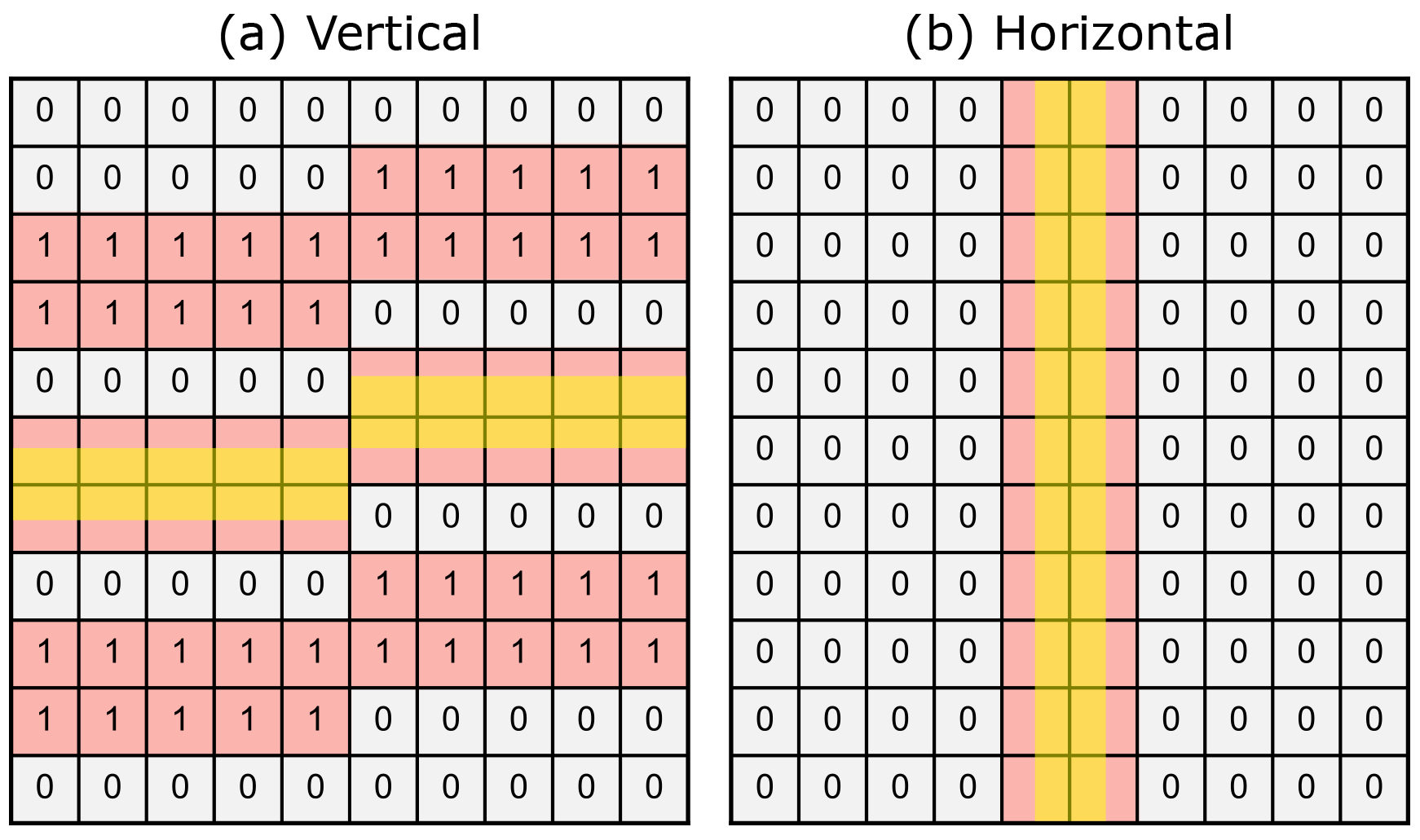
Figure 3Vertical (a) and horizontal (b) difference matrix D showing all cells (red) in the shifted matrices S1 and S2, which are next to the interface between two different layers or of any layers across a fault. The highlighted (yellow) part shows the area in which the implicit interface must be located.
2.3 Stochastic modeling approach
2.3.1 Bayesian inference
Bayesian inference is fundamentally different to the classical frequentist approach of inference. It treats probabilities as degrees of certainty of a parameter θ, which is inherently considered to be a random variable itself (Bolstad, 2009; VanderPlas, 2014). It is based on Bayes' theorem (Eq. 2), which allows updating of a given probability – the prior probability p(θ) of a parameter θ – after the occurrence of a connected event (Bolstad, 2009). This updating process relies on the use of a likelihood function p(y|θ), representing the conditional probability of the observed data y given the prior probability of the underlying parameter θ and the theoretical connection of the occurring event. It is used to condition the prior into the posterior distribution p(θ|y), which represents the degree of certainty over the parameter θ given the occurrence of the event and its observed data y.
In this paper, we consider Bayes' equation as a general way to combine conditional probabilities as in the interpretation of, for example, probabilistic graphical models (Koller et al., 2009). For use in geomodeling, the terms in Eq. (2) can be seen as (de la Varga and Wellmann, 2016; Gelman et al., 2013) follows.
-
Model parameters, θ, are model-defining parameters (e.g., layer interface positions, dip or fault parameters) used for the interpolation of the geomodel, which can be either deterministic (thus be exactly defined and known) or probabilistic. The latter represent uncertain parameters, which is expressed in the form of probability distributions (e.g., a normal distribution expressing the uncertainty of the vertical subsurface position of a layer interface). We will use θ′ as the notation for a sample from these parameter distributions.
-
Observed data: y represents additional measurements or any other source of data, which should enhance the model definition by providing additional information with the goal of reducing model uncertainty or enabling the comparison of the model to reality (e.g., by comparing geophysical potential-field measurements with the according forward simulation on the basis of a geomodel). In this work we use topology information in the form of a topology adjacency graph as the observed data. Notice that when the terms “observation” or “observed data” are used in the context of a probabilistic model, we refer to this mathematical term y instead of to the literal semantic meaning of the words.
-
Likelihood functions, p(y|θ): these form the relationship between the model parameters θ and the observed data y. Essentially, this function describes the conditional probability for observing the data y given the parameters θ (e.g., MacKay and Kay, 2003). In the case of structural modeling, this essentially means that we compute the geomodel from the input parameters θ and compare model predictions (e.g., the thickness of a certain layer at a certain position or topology adjacency graphs) with additional observed data.
While constructing meaningful likelihood functions for physical properties such as layer thickness or geobody volume from observed data is straightforward (de la Varga and Wellmann, 2016), we have no proper framework to construct them for more abstract or “soft data”, such as our understanding of the geological setting or the topology relationships of our layers across faults or unconformities. For this reason, we chose to apply methods to estimate our posterior distributions given abstract geological information without specifying a likelihood function: approximate Bayesian computation.
2.3.2 Approximate Bayesian computation
Geoscientists often have extensive implicit knowledge of geological settings (e.g., our understanding of the tectonics of a system), but only a limited amount of this knowledge can be incorporated into the geological interpolation function (Wellmann and Caumon, 2018). Additionally, it is often difficult to define formal likelihood functions for geological knowledge as required for conventional Bayesian inference methods (Wood and Curtis, 2004). A less formal but valid alternative approach is to approximate the posterior distributions using approximate Bayesian computation (ABC) methods. These methods, also referred to as likelihood-free inference methods by some (Marin et al., 2012), evaluate the distance of stochastically generated models to our additional data using one or multiple summary statistics, S, instead of a probabilistic likelihood function. While summary statistics are often measures such as the mean, mode or median of a model, they tend to be insufficient in summarizing geomodels. In this work we use the geomodel topology graph as a summary statistic of the geomodel to provide a meaningful comparison between geomodels.
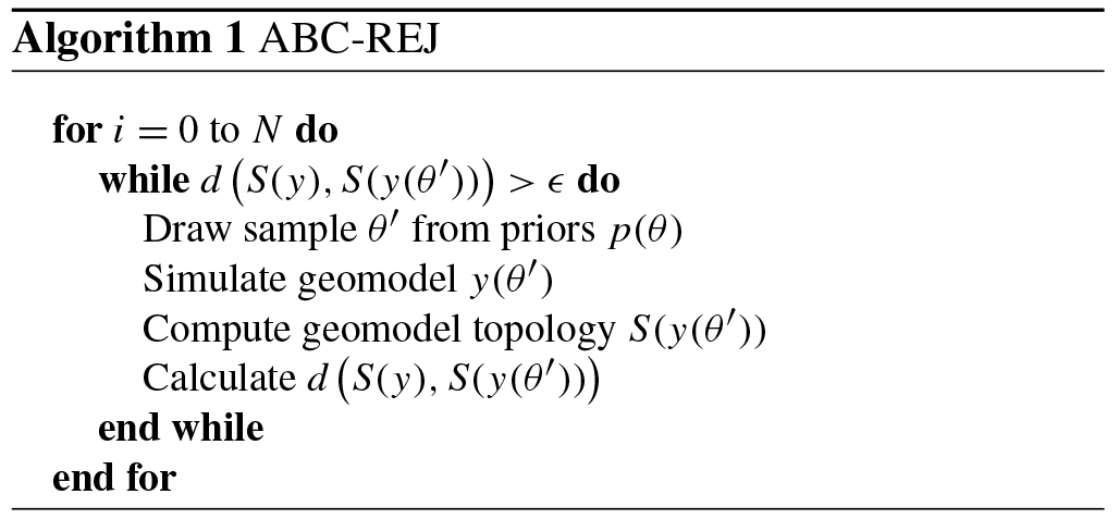
To obtain the approximate posterior distribution we need to sample from our prior parameter distributions, plug the sample values θ′ into our simulator function y (our geomodeling software), compute the summary statistic S(y(θ′)) (geomodel topology) and evaluate its distance to our observed summary statistic (data) S(y) (e.g., a geomodel topology graph). The most fundamental sampling scheme for ABC is based on rejection sampling (ABC-REJ; see Algorithm 1), for which the distance between our simulated data y(θ′) (the simulated geomodel) and observed data y (initial geomodel) is calculated using a distance function of their summary statistics (topology graphs) . The simulated model is accepted if the distance is below a user-specified error bound ϵ≥0 (Sadegh and Vrugt, 2014); otherwise, it is rejected. The accepted samples form the approximate posterior. Thus, this method circumvents the need to specify a likelihood function for our additional data, while still approximating the posterior distributions incorporating the information of both our priors and our additional information (Sunnåker et al., 2013). Within this work we use the Jaccard index (1−J) as a distance function between topology graphs.
A more advanced sampling scheme for ABC is sequential Monte Carlo sampling (ABC-SMC). In its simplest form it can be seen as an extension of rejection sampling by chaining rejection sampling simulations together (each referred to as an epoch). During the first epoch of rejection sampling, a large error threshold ϵ1 is used while sampling from the prior distributions p(θ). The accepted samples, forming the posterior distributions of the first epoch, form the updated priors of the second epoch by replacing the priors with the kernel density estimation of the posterior samples. Iteratively, with every epoch, the error threshold ϵ is reduced to the target value (e.g., ϵ=0) to obtain the final posterior sample. Thus, every epoch, the sampler “learns” from the previous epoch by adjusting the prior distributions further towards the posterior distributions. As ABC-REJ tends to suffer from potentially low computational efficiency when using low error thresholds ϵ, the iterative shrinking paired with adjustment of the prior distributions can potentially obtain the approximate posterior much more quickly. We apply this sampling scheme to our Gullfaks case study to show the potential speed-ups.
2.4 Topology distance functions
To use geomodel topology as a constraint for probabilistic geomodels in an ABC framework, we need a consistent way of comparing geomodel topologies – i.e., suitable distance functions. We consider three possible comparison methods here.
-
Presence or absence of defined connections. As the relational topology information is captured in adjacency graphs, the most fundamental approach is to check if two relevant nodes n1 and n2 (e.g., representing two regions in the model) share an edge (are adjacent) and if this edge exists in both models. This is the most simple way of comparing specific aspects of relational topology between geomodels. This approach can be viewed as a Boolean comparison that is true if the given edge exists in both models and false if not. This also enables the direct comparison of i multiple edges, which would result in a vector of i Boolean statements for each comparison .
-
Comparing entire graphs. To compare topology graphs as a whole, Thiele et al. (2016b) describe the use of the Jaccard index (Jaccard, 1912). It can be used to compare the similarity of sets by creating the ratio of the intersection and union of two graphs A and B.
For two topology graphs A and B, this means we calculate the ratio of edges (representing connected regions) shared in both (intersection: A∩B) and their total combined number of edges (union: A∪B). This ratio can be used to efficiently identify all unique topology graphs in a given ensemble, as only an identical pair of graphs results in a Jaccard index of . A comparison using the Jaccard index yields ratios of integers and thus a discrete comparison. This method also allows specifying a tolerance for model acceptance, i.e., to accept models within the range .
-
Contact area. Comparing the number of actual edge pixels (or voxels) representing the area of the contact Ae between two geobodies could yield a more granular comparison that allows us to take into account trends of the contact size. Thus, the ABC error tolerance ϵ could be used to reject geomodels wherein certain topological contact areas are above and/or below a certain value: .
In this work we demonstrate the second approach, as it allows us to directly compare entire geomodel topologies. We have chosen to compare the simulated results to a single topology graph – the initial geomodel topology. This approach was selected as a base case to demonstrate how large variations in geomodel topology observed in the stochastic simulation of input data uncertainties in geomodels (see Thiele et al., 2016b) can be constrained to a base topology (i.e., conceptual model). This of course reinforces the bias of the initial base model in the uncertainty simulation, but it allows for the reliable exploration of the uncertainty of all possible geomodels honoring the topology constraint.
2.5 Quantifying uncertainty using Shannon entropy
Stochastic simulations yield vast ensembles of geomodel realizations, and their variability (and thus uncertainty) needs to be analyzed and understood. The uncertainty of a single geological entity (e.g., a layer or a fault) can be estimated from its frequency of occurrence in each single geomodel voxel. In order to analyze the whole geomodel uncertainty at once, more sophisticated measures can be applied: the concept of Shannon entropy H can be used in a spatial context to evaluate the uncertainty of an entire geomodel ensemble at once, as described by Wellmann and Regenauer-Lieb (2012). Average model entropy collapses the uncertainty of a geomodel ensemble into a single number. It will be equal to 0 if all cells x have only one possible outcome (no uncertainty) and reach its maximum when all outcomes are equally likely for all cells of the model (maximum uncertainty).
Figure 4(a) 3-D view of the synthetic fault model, with top surfaces of the four lithologies shown and the fault surface in blue. (b) X–Z slice through the center of the discretized model showing partial input data (for visual brevity) and example standard deviations of prior parameters used for the stochastic simulation. (c) Model overlaid with its topology graph used as our summary statistic for the ABC.
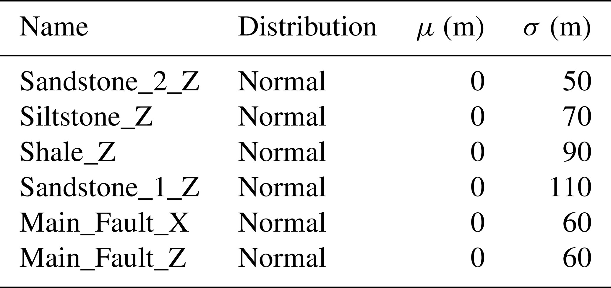
Table 1Distribution parameters for prior parameterization of the synthetic fault model.
2.6 Experiment design
2.6.1 Synthetic fault model
As a proof of concept we show how ABC can be used to incorporate geological knowledge and reasoning into an uncertain synthetic geomodel. This model represents a folded layer cake stratigraphy that is cut by a N–S-striking normal fault to represent an idealized reservoir scenario frequently encountered in the energy industry (see Fig. 4a).
The prior parameterization is schematically visualized in Fig. 4b and consists of two different kinds of uncertain parameters: (i) vertical location of the layer and fault interfaces and (ii) lateral location of the fault interface, with the specific parameterization displayed in Table 1. As this work focuses on developing and describing a novel methodology for constraining uncertain geomodels, we have chosen the uncertainty parameterization of the synthetic geomodel entirely subjectively as normal distributions increasing in uncertainty with depth. The uncertainty is individually applied to each set of surface points to preserve surface shape within each of the two fault blocks. Proper prior parameterization of uncertain geomodels is a vital branch of research on its own (e.g., Pakyuz-Charrier, 2018; Krajnovich et al., 2020) and out of the scope of this work.
Two separate simulations were run for this experiment so we can see how topology can constrain an uncertain geomodel compared to the Monte Carlo simulation of input parameter uncertainties alone.
-
A Monte Carlo simulation of the prior parameters was run to evaluate the uncertainty in the resulting geomodel ensemble consisting of 2000 generated models. This represents our “base case” uncertainty without any topological constraints. It is important to note that this simulation is only a forward uncertainty propagation and does not entail any type of inference.
-
An approximate Bayesian computation was done using the initial model topology graph (see Fig. 4c) to represent our geological knowledge. This graph is extracted from the initial geological model, which has been manually built by an expert. The assumption is that this topological graph encapsulates important aspects of the geological knowledge used during its construction, and thus geometrical configurations more similar to this graph can be considered more likely (see also Thiele et al., 2016b; Pakyuz-Charrier et al., 2019). This graph would be treated from this point on as an “observation” y due to its use as a constraint within the probabilistic model. We are employing a rejection sampling scheme (ABC-REJ) with an error tolerance of ϵ=0 to obtain 500 generated posterior models. The resulting posterior geomodel ensemble will contain only samples with matching topology graphs.
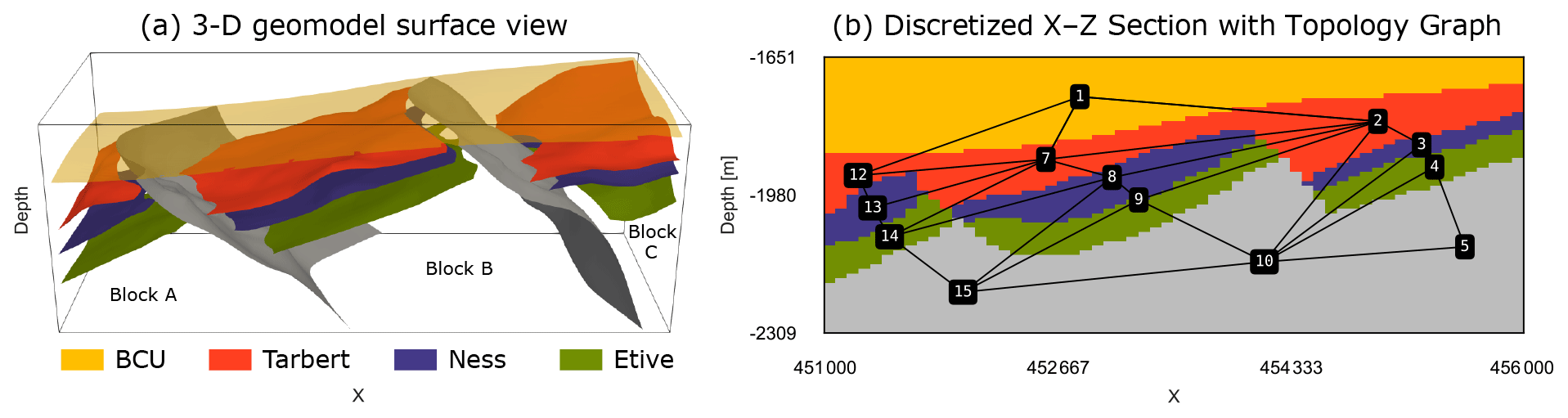
Figure 5(a) 3-D view of the Gullfaks geomodel used as the mean prior model in our case study. (b) X–Z section through the discretized geomodel with an overlaid observed topology graph showing the inter- and intra-fault block relations of geobodies.
2.6.2 Case study: the Gullfaks field
To demonstrate the applicability of the method to real datasets we apply it to a model of part of the Gullfaks field, located in the northern North Sea. The field is located in the western part of the Viking Graben and consists of the NNE–SSW-trending 10–25 km wide Gullfaks fault block (Fossen and Hesthammer, 1998). For a detailed overview of the regional and structural geology we refer to Fossen and Rørnes (1996), Fossen and Hesthammer (1998), Fossen et al. (2000), and Schaaf and Bond (2019).
For the experiment, we constructed a base geomodel (Fig. 4a)
founded in an interpretation of the training dataset provided with the seismic
interpretation software Petrel™. We have chosen a
relatively simple subset of the interpretation containing two faults, three
horizon tops (Tarbert – red, Ness – purple and Etive – green) and the Base
Cretaceous Unconformity (BCU, yellow). To create the geomodel, we exported the
corresponding seismic interpretation data from Petrel and imported them into
Python. The surface interpretations were then decimated down to 510 surface
points and 187 surface orientations via a target reduction of 80 % per
fault block or surface using the VTK-based decimation functionality of
pyvista (Sullivan and Kaszynski, 2019) to retain the best possible
surface shape while allowing fast implicit geomodel construction times in
GemPy.
Table 2Distribution parameters for prior parameterization of the Gullfaks case study.
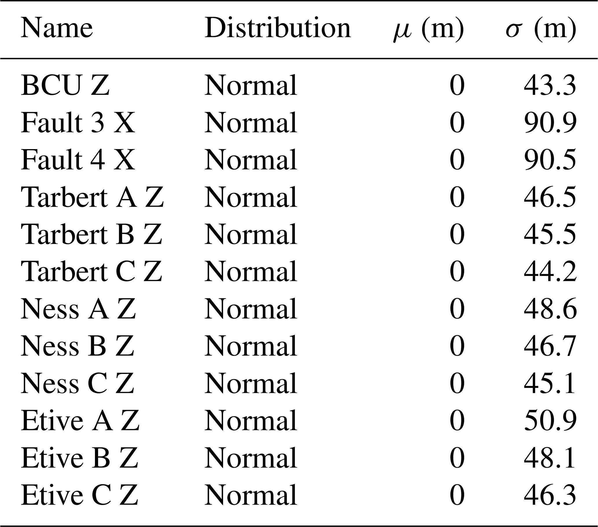
The prior parameterization consists of two different kinds of uncertain parameters: (i) vertical location of the layer interfaces within each fault block and (ii) the lateral location of the fault interfaces. This parameterization is similar to the synthetic fault model (all specifications are listed in Table 2), and all sets of surface points within each individual fault block were perturbed together to retain surface shape. This parameterization was chosen to demonstrate how even a few uncertain parameters in an uncertainty modeling workflow can lead to highly uncertain results, especially regarding the topology graphs of the resulting geomodel ensembles in real-world geomodels. We then conducted a sensitivity study of the topological spread with respect to the geomodel resolution. This allowed us to determine the appropriate geomodel resolution necessary for our experiment. Next, we performed three separate simulations to compare different approaches.
-
A Monte Carlo simulation was run of the prior uncertainty for 1000 samples to evaluate the spatial uncertainty and the topological spread of the resulting geomodel ensemble. This serves as our base case uncertainty for comparison with the following two simulations.
-
An ABC-REJ simulation was run using the initial geomodel topology graph (see Fig. 4b) to represent our geological knowledge. We used an error threshold of ϵ=0.025 for 1000 accepted posterior samples, as the threshold was small enough to constrain the posterior topology spread to the initial geomodel topology graph.
-
An ABC-SMC simulation was run using the same initial geomodel topology graph. We ran six SMC epochs using ϵ values of 0.3, 0.2, 0.1, 0.075, 0.05 and 0.025. Each epoch was run for 1000 accepted posterior samples.
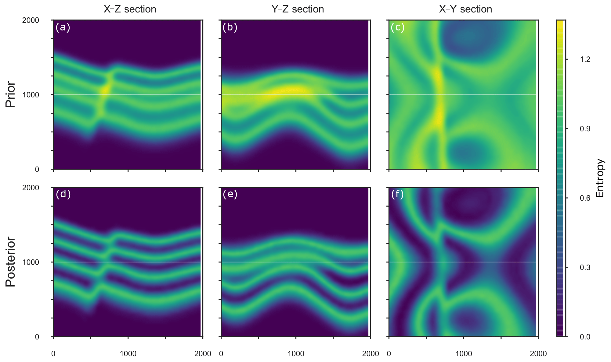
Figure 6Shannon entropy slices in the X–Z (a, d), Y–X (b, e) and X–Y plane of the prior (top, a–c) and posterior (bottom, d–f) geomodel ensemble. The white lines show the location of other respective cross sections.
3.1 Synthetic fault model
Simulating the uncertainties encoded in the prior parameterization resulted in 100 unique model topologies within the geomodel ensemble of 2000 models, with 18 topology graphs occurring at least 10 times and the most frequent 14 making up 90 % of geomodel ensemble topologies. It is also notable that the most frequent topology graph (29.5 %) is not the initial (mean prior) topology graph (15.6 %), but rather represents models wherein the shale layer (green) of the footwall shares an across-fault connection with the sandstone 2 layer (red) of the hanging wall. The uncertainty of the prior geomodel ensemble is visualized in Fig. 5a–c in X–Z, Y–Z and X–Y sections as Shannon entropy, as described in the Methodology section. All three sections through the model clearly show the uncertainty of the layer interface position and the highest uncertainty around the fault surface. In comparison, applying a single topology graph as a summary statistic to the simulation using ABC leads to significantly reduced uncertainty throughout the geomodel ensemble (see Fig. 5d–f), with average geomodel ensemble entropy being reduced from down to , which is a drop in geomodel uncertainty of nearly 30 %. Visualizing the entropy difference between the prior and the posterior geomodel ensembles shows the highest reduction in entropy for the two inner layer interfaces (see Fig. 6) and not around the fault surface. As expected, constraining the simulation using a single topology graph with an error of ϵ=0 collapses the number of geomodel ensemble topologies from 100 down to 1.
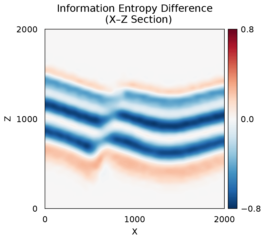
Figure 7X–Y section of entropy difference between the forward simulated entropy and the approximate posterior entropy. The plot highlights areas where the entropy was reduced (blue), increased (red) and kept constant (white).
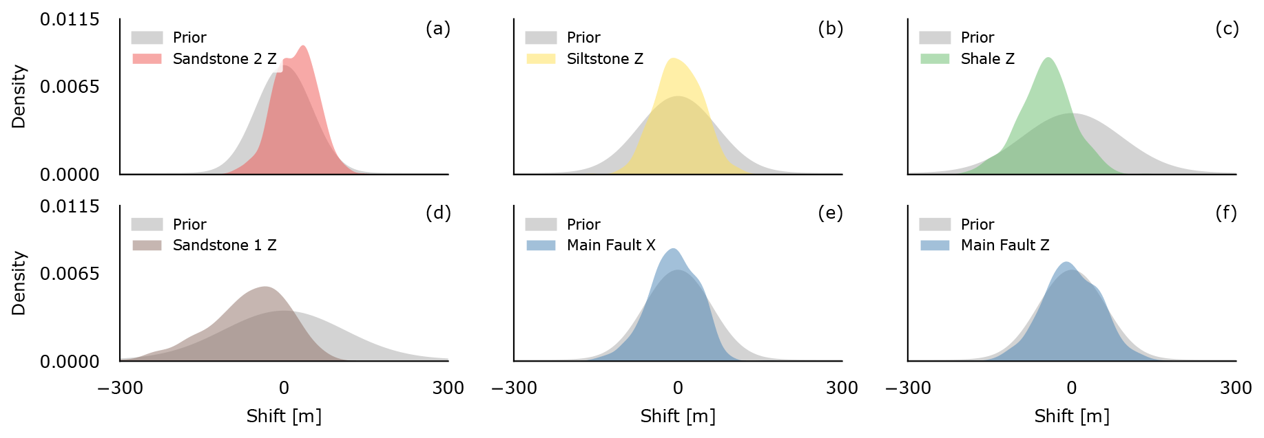
Figure 8Prior (grey) and posterior (color) kernel density estimations for the different stochastic model parameters for our synthetic fault model.
Figure 7 plots the kernel density estimations (KDEs) of the input parameter distributions of prior (grey) and posterior (colored) samples. The strongest change in the mean from prior to posterior distributions occurred for the vertical interface location perturbation priors of sandstone 2 (red), shale (green) and sandstone 1 (brown; see Fig. 7), with the first shifted to higher mean z values and the latter two shifted deeper by −72 and −53 m, respectively. Additionally, the initially normally distributed prior of sandstone 1 shows a strong negative skewness of −0.61 in the posterior distribution. The standard deviation for the siltstone and shale interface distributions was reduced by roughly 32 % and 40 %, respectively. The prior and posterior distributions for the lateral and vertical fault parameter uncertainties show no significant difference (panels e and f).
3.2 Case study: the Gullfaks field
Forward simulation of the prior uncertainties of the Gullfaks geomodel resulted in 676 unique geomodel topologies within a 1000-model ensemble, with 116 unique topologies occurring more than once. Again, the most frequent topology graph is not the initial (mean prior) topology graph. The uncertainty of an X–Z section of the forward ensemble is visualized in Fig. 9a using Shannon entropy. The section illustrates the general trend of uncertainty throughout the forward simulation: we observe the highest uncertainty surrounding the two faults in the geomodel, especially around the eastern fault. The area also shows increased uncertainty due to the interaction of layer interfaces, the fault and the vertical vicinity of the BCU.
The initial topology graph is used as a constraining summary statistic using ABC with rejection sampling (ABC-REJ) and a threshold of ϵ=0.025. The absolute threshold value will be directly proportional to the sensitivity of the model geometry with respect to the stochastic parameters. This prevents the selection of a value independent of the actual geological model under study. In this case study, the value of ϵ has been chosen empirically by performing several predictive simulations. Results were evaluated based on their correspondence to the geological setting, as judged by expert knowledge.
The results shows that this approach leads to reduced uncertainty, as exemplified by the entropy section shown in Fig. 9b. At this threshold, the approximate posterior geomodel ensemble contains only the applied initial topology graph. Using rejection sampling with such a strict threshold resulted in a very low acceptance of only 0.59 % of simulated geomodels, which required about 40 h of simulation time to obtain 1000 posterior samples2. In contrast, using a sequential Monte Carlo sampling scheme (ABC-SMC) required only 3.96 h to obtain the same number of posterior samples at the same threshold – a speed-up of 10.1. This includes the five sampling epochs using with 1000 accepted samples each, which are used to sequentially adapt the priors.
Figure 11a shows the number of unique topologies for forward simulations and each threshold of the ABC-SMC. As we iteratively lower the acceptable threshold during the SMC simulation, the simulated and accepted topologies iteratively converge towards the topology graph we used as our prior geological knowledge. The average geomodel ensemble entropy also iteratively decreases from 0.233 for the forward simulation down to 0.112 at ϵ=0.025 (see Fig. 11b), showing how fixing a probabilistic geomodel to a single topology graph can significantly reduce, or rather significantly constrain, the simulated uncertainty.
Figure 8 shows how the ABC-SMC simulation iteratively affects the probability distributions of selected probabilistic geomodel parameters with decreasing thresholds ϵ. Each row shows the consecutive epochs of the ABC-SMC simulation and corresponds to a specific ϵ. Each column describes a different stochastic parameter in the stochastic model. By applying the initial topology graph of the geomodel as our summary statistics, we can directly see here how the parameter distribution for the BCU (Fig. 8a) shifts its mean μ by 47.4 m upwards and reduces its standard deviation σ by 35.8 % to accommodate our geological knowledge about the geomodel topology. We can observe this effect in the entropy section of the posterior geomodel ensemble as well (Fig. 9b). In Fig. 10, we show the difference in entropy between the prior and approximate posterior geomodel ensemble shown in Fig. 9, where areas with decreasing entropy values are shown in blue and increasing values in red. We observe here how the BCU moves upward and increases the entropy there, while lowering entropy in the lithologies below. The parameter distributions for Tarbert B (Fig. 8b, red) and Etive B (Fig. 8c, green) show similar behavior: a shifted mean and reduced standard deviation to accommodate the topology information. We see a much stronger reduction in standard deviation for the two faults (Fig. 8d, e): 80.4 % and 80.0 % for Fault A and Fault B, respectively. This is also shown as the strongest reduction in entropy in Fig. 10.
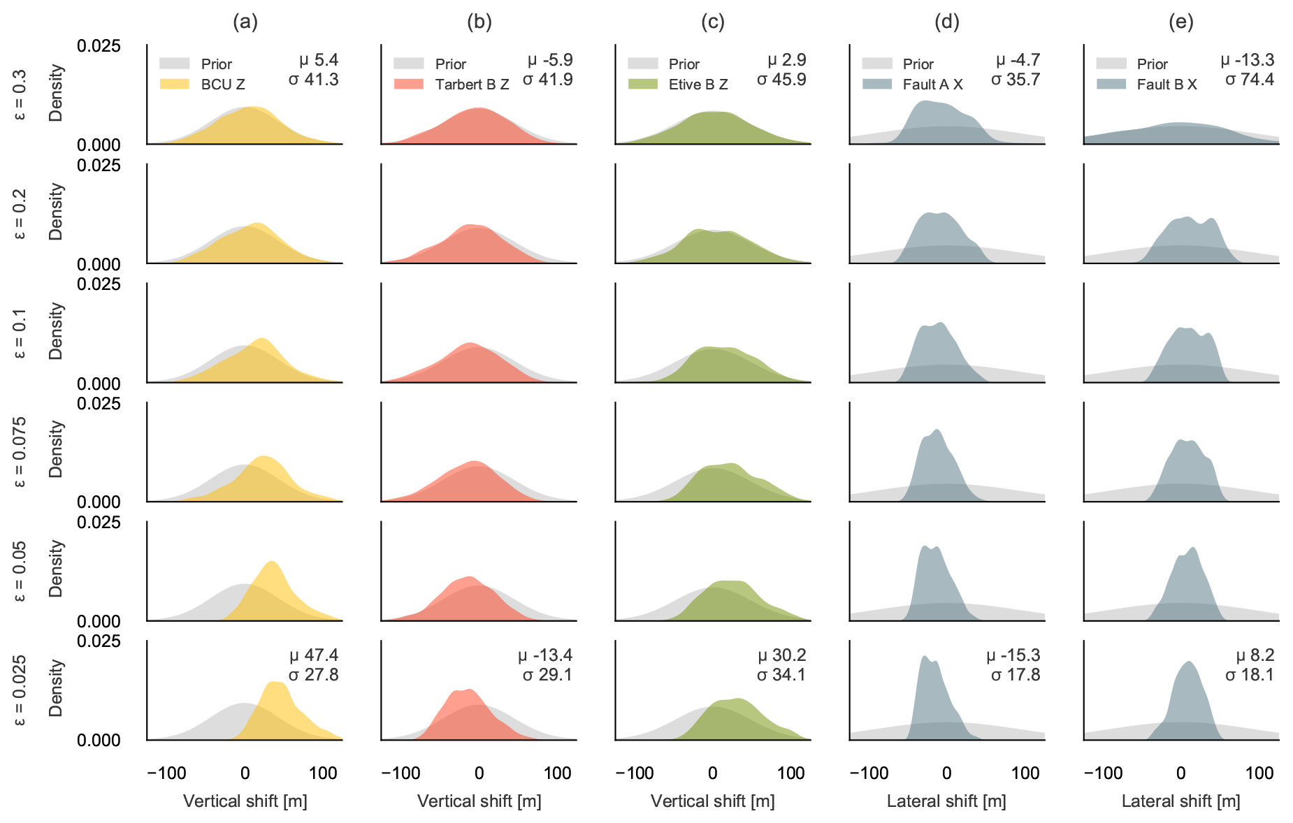
Figure 9Prior (grey) and posterior (colored) kernel density estimations for selected model parameters (a–e) for the six epochs (each row represents an epoch) of the ABC-SMC simulation of the Gullfaks case study, showing how the simulation iteratively approaches the approximate posterior distribution, which shows the possible parameter uncertainty given our topological information. The mean μ and standard deviation σ are shown for the first and last epochs.
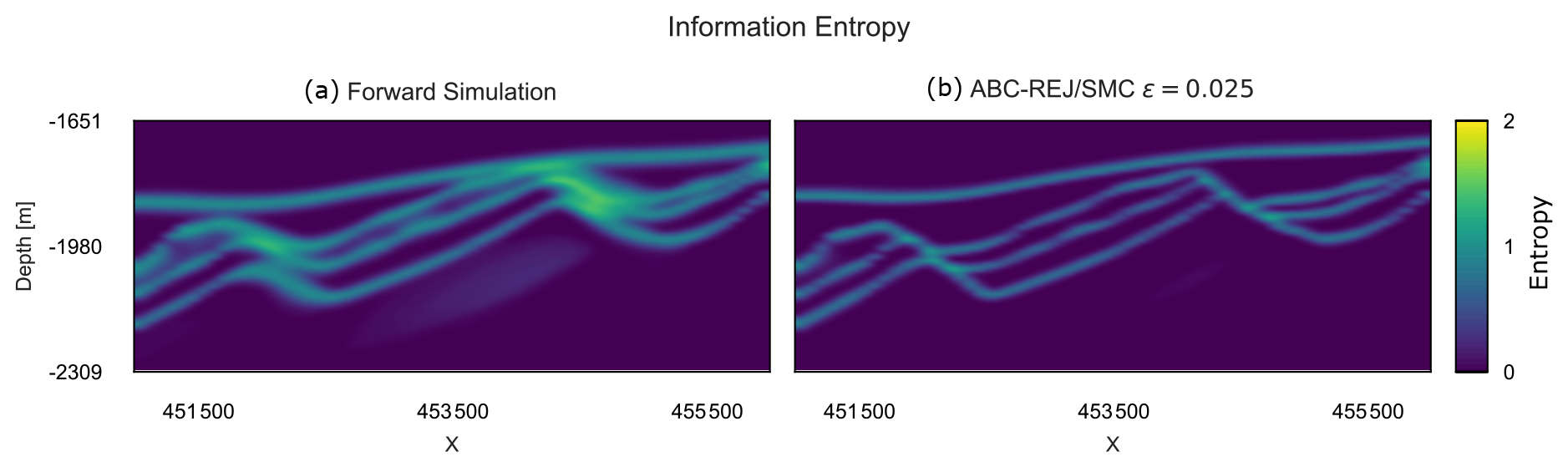
Figure 10(a) Section of the entropy block of the forward simulation for the prior uncertainty (HT=0.223). (b) Section of the entropy block of the final epoch (ϵ=0.025) of the ABC-SMC simulation (HT=0.113).
Figure 11X–Z section of entropy difference between the forward-simulated entropy and the approximate posterior entropy H (ϵ=0.025). The plot highlights areas where the entropy was reduced (blue), increased (red) and kept constant (white).
Figure 12(a) Number of unique topologies within the geomodel ensembles of each SMC epoch, showing the iterative reduction in topological uncertainty throughout the SMC simulation. (b) Average geomodel entropy of the ensembles for each epoch, showing how the reduction of topological uncertainty shown in (a) affects the total geomodel uncertainty.
We showed how topology information, as an encoding for important aspects of geological knowledge and reasoning, can be included in probabilistic geomodeling methods in a Bayesian framework. The simulation experiments for our two case studies demonstrated that we are able to approximate posterior distributions to obtain probabilistic geomodel ensembles that honor both our prior parameter knowledge and qualitative geological knowledge. If the applied topological information is meaningful, then the constrained stochastic geomodel ensemble will see a meaningful reduction in uncertainty and will subsequently allow for more precise model-based estimates and decision-making (Stamm et al., 2019). More importantly, the (approximate) Bayesian approach requires the explicit statement of the geological knowledge (here the topology information) used in the probabilistic geomodel, increasing the transparency of assumptions made during the geomodeling process and any subsequent decisions.
With our approach, we directly address a scientific challenge raised in recent work by Thiele et al. (2016b) that known topological relationships are frequently not honored during the probabilistic modeling process, thus potentially invalidating large parts of the resulting geomodel ensemble. Injecting topology information into a Bayesian approach allows us to obtain topologically valid, and hence geologically reasonable, geomodel ensembles. And, although we have only used simple topology information within this study, the demonstrated ABC approach allows us to easily scale the amount of topology information used: from simple true–false comparisons of single topology graphs to the use of a whole range of topology graphs and relationships. If a set of acceptable topologies is used, one could, for example, accept a simulated model if it matches at least one within the error tolerance.
The work of Pakyuz-Charrier et al. (2019) shows how clustering of probabilistic geomodel topologies can be used to differentiate between different modes of topologies. Their approach compares geomodel topologies by describing them as half-vectorized adjacency matrices, resulting in a binary string that can be compared using the Hamming distance (Hamming, 1950). It could be considered as a different distance metric in the ABC approach presented in this work to constrain the simulated probabilistic geomodel. And, while their work focuses on the analysis of existing probabilistic geomodel ensembles, our approach focuses on training probabilistic geomodels on topology information.
As more complex geomodels strongly increase the required parameterization to accurately describe the model domain in a probabilistic framework, constraining them with topological information could help keep this parameterization at computationally feasible levels by reducing the parameter dimensionality, while still obtaining meaningful geomodels (e.g., free of modeling artifacts caused by random perturbations of the limited input data). This would not work using an inefficient rejection sampling scheme (e.g., ABC-REJ) but would rather require the use of “adaptive” sampling algorithms to efficiently explore the posterior parameter space without wasting too much computing power on rejected models (e.g., ABC-SMC). In our Gullfaks case study, we have not only shown the efficacy of the method in a real-world example, but have also demonstrated the stark increase in computational efficiency when using advanced sampling techniques. The SMC sampler used in our work requires manual setting of the acceptance thresholds, which directly influence the algorithm's efficiency in acquiring samples of the approximate posterior distribution. Adaptive SMC methods automatically tune acceptance thresholds to increase sampling efficiency “on the fly” to minimize computation time and avoid manual (subjective) selection of thresholds (Del Moral et al., 2012).
Sadegh and Vrugt (2014) describe a more complex ABC algorithm based on Differential Evolution Adaptive Metropolis (DREAM-ABC) and demonstrate its much higher efficiency in approximating the posterior. It might be of particular interest for the approximate inference of complex structural geomodels with topology constraints, as it has shown promise to very efficiently explore high-dimensional (read: large amount of prior parameters) and multi-modal parameter spaces. When using multiple topology graphs (which are discrete) in an ABC framework, the posterior parameter space may potentially become multi-modal, which poses significant challenges for traditional Markov chain-based samplers (Feroz and Hobson, 2008). The approach by Sadegh and Vrugt (2014) is based on combining multiple Markov chains, which natively supports parallel computing and would thus allow for a high scalability of the approach to complex, computationally intensive geomodels.
Alternatively, Bayesian optimization for likelihood-free inference (BOLFI; Gutmann and Corander, 2016) could be worth considering for complex structural geomodels. The method abstracts the simulator and/or implicit function into a statistical surrogate model between the priors and the summary statistics and then attempts to minimize their distance, with the potential to significantly reduce the number of needed computations of the geomodel. Overall, the spatial and discrete nature of geomodels and the use of discrete summary statistics pose unique challenges for sampling algorithms, requiring further research to identify algorithms that can confidently converge and minimize the high computational cost of probabilistic 3-D geomodels.
The method demonstrated the effect of topology information on geomodel uncertainty – showing how well the parameterization of a probabilistic geomodel fits our geological assumptions. The acceptance rates during sampling could potentially be used as a proxy for the validity of our assumptions: low acceptance rates could reveal a bad fit between our model and our added geological knowledge and reasoning. Using entropy-difference plots, the effect of geological assumptions on geomodel uncertainty can be analyzed spatially, e.g., how it changes around faults and other structures in the geomodel ensemble.
-
We have shown how to use approximate Bayesian computation to constrain probabilistic geomodels so that the approximate posterior incorporates known topology information.
-
The method enables additional geological knowledge and reasoning to be explicitly encoded and incorporated into probabilistic geomodel ensembles, potentially increasing the transparency of the modeling assumptions.
-
As opposed to standard MC with rejection, the implemented SMC approach makes the use of ABC feasible in realistic settings. Further research into using more advanced sampling schemes could provide additional speed-ups in obtaining the posterior geomodel ensemble, which is especially relevant for computationally more expensive complex geomodels with large parameterizations.
AS was responsible for the data curation, investigation, validation and visualization. Conceptualization, design and development of the research's methodology were done by AS, MdlV and FW. Formal analysis and software development were done by AS and MdlV. Supervision, research resources and funding acquisition were provided by CB and FW. AS was responsible for writing the original draft, while all authors contributed to the review and editing process.
The authors declare that they have no conflict of interest.
Publisher's note: Copernicus Publications remains neutral with regard to jurisdictional claims in published maps and institutional affiliations.
We would like to thank Total E&P UK in Aberdeen for funding this research. We also thank Fabian Stamm for providing the wonderful synthetic geomodel used in this paper. We are grateful for the constructive reviews from Ashton Krajnovich and an anonymous reviewer for helping us improve this paper.
This research was conducted within the scope of a Total E&P UK-funded postgraduate research project.
This paper was edited by Thomas Poulet and reviewed by Ashton Krajnovich and one anonymous referee.
Baddeley, M. C., Curtis, A., and Wood, R.: An introduction to prior information derived from probabilistic judgements: elicitation of knowledge, cognitive bias and herding, Geological Society, London, Special Publications, 239, 15–27, 2004. a
Bardossy, G. and Fodor, J.: Evaluation of Uncertainties and Risks in Geology: New Mathematical Approaches for Their Handling, Springer Science & Business Media, 2013. a
Bistacchi, A., Massironi, M., Dal Piaz, G. V., Dal Piaz, G., Monopoli, B., Schiavo, A., and Toffolon, G.: 3D Fold and Fault Reconstruction with an Uncertainty Model: An Example from an Alpine Tunnel Case Study, Comput. Geosc., 34, 351–372, https://doi.org/10.1016/j.cageo.2007.04.002, 2008. a
Bolstad, W. M.: Understanding Computational Bayesian Statistics, John Wiley & Sons, 2009. a, b
Bond, C., Gibbs, A., Shipton, Z., and Jones, S.: What Do You Think This Is? “Conceptual Uncertainty” in Geoscience Interpretation, GSA Today, 17, 4, https://doi.org/10.1130/GSAT01711A.1, 2007. a, b
Bond, C. E.: Uncertainty in structural interpretation: Lessons to be learnt, J. Struct. Geol., 74, 185–200, 2015. a
Bond, C. E., Shipton, Z. K., Gibbs, A. D., and Jones, S.: Structural models: optimizing risk analysis by understanding conceptual uncertainty, First Break, 26, 6, https://doi.org/10.3997/1365-2397.2008006, 2008. a
Brandes, C. and Tanner, D. C.: Fault-related folding: A review of kinematic models and their application, Earth-Sci. Rev., 138, 352–370, 2014. a
Butler, R. W., Bond, C. E., Cooper, M. A., and Watkins, H.: Interpreting structural geometry in fold-thrust belts: Why style matters, J. Struct. Geol., 114, 251–273, 2018. a
Calcagno, P., Chilès, J. P., Courrioux, G., and Guillen, A.: Geological Modelling from Field Data and Geological Knowledge: Part I. Modelling Method Coupling 3D Potential-Field Interpolation and Geological Rules, Phys. Earth Planet. In., 171, 147–157, https://doi.org/10.1016/j.pepi.2008.06.013, 2008. a
Chilès, J. P., Aug, C., Guillen, A., and Lees, T.: Modelling the Geometry of Geological Units and Its Uncertainty in 3D From Structural Data: The Potential-Field Method, Proceedings of international symposium on orebody modelling and strategic mine planning, Perth, Australia, 22, 24 pp., 2004. a
Crossley, M. D.: Essential Topology, Springer Science & Business Media, 2006. a
Curtis, A. and Wood, R.: Optimal Elicitation of Probabilistic Information from Experts, Geological Society, London, Special Publications, 239, 127–145, https://doi.org/10.1144/GSL.SP.2004.239.01.09, 2004. a
de la Varga, M. and Wellmann, J. F.: Structural Geologic Modeling as an Inference Problem: A Bayesian Perspective, Interpretation, 4, SM1–SM16, https://doi.org/10.1190/INT-2015-0188.1, 2016. a, b, c
de la Varga, M., Schaaf, A., and Wellmann, F.: GemPy 1.0: open-source stochastic geological modeling and inversion, Geosci. Model Dev., 12, 1–32, https://doi.org/10.5194/gmd-12-1-2019, 2019. a, b
Del Moral, P., Doucet, A., and Jasra, A.: An Adaptive Sequential Monte Carlo Method for Approximate Bayesian Computation, Stat. Comput., 22, 1009–1020, https://doi.org/10.1007/s11222-011-9271-y, 2012. a
Egenhofer, M. J.: Categorizing binary topological relations between regions, lines, and points in geographic databases, Santa Barbara CA National Center for Geographic Information and Analysis Technical Report, 9, 76 pp., 1990. a
Feroz, F. and Hobson, M. P.: Multimodal Nested Sampling: An Efficient and Robust Alternative to Markov Chain Monte Carlo Methods for Astronomical Data Analyses, Mon. Not. R. Astron. Soc., 384, 449–463, https://doi.org/10.1111/j.1365-2966.2007.12353.x, 2008. a
Fossen, H.: Structural Geology, Cambridge University Press, 1st Edn., 2010. a
Fossen, H. and Hesthammer, J.: Structural Geology of the Gullfaks Field, Northern North Sea, Geological Society, London, Special Publications, 127, 231–261, https://doi.org/10.1144/GSL.SP.1998.127.01.16, 1998. a, b
Fossen, H. and Rørnes, A.: Properties of Fault Populations in the Gullfaks Field, Northern North Sea, J. Struct. Geol., 18, 179–190, https://doi.org/10.1016/S0191-8141(96)80043-5, 1996. a
Fossen, H., Odinsen, T., Færseth, R. B., and Gabrielsen, R. H.: Detachments and Low-Angle Faults in the Northern North Sea Rift System, Geological Society, London, Special Publications, 167, 105–131, https://doi.org/10.1144/GSL.SP.2000.167.01.06, 2000. a
Frodeman, R.: Geological Reasoning: Geology as an Interpretive and Historical Science, Geol. Soc. Am. Bull., 107, 960–0968, https://doi.org/10.1130/0016-7606(1995)107<0960:GRGAAI>2.3.CO;2, 1995. a
Gelman, A., Carlin, J. B., Stern, H. S., Dunson, D. B., Vehtari, A., and Rubin, D. B.: Bayesian Data Analysis, Chapman and Hall/CRC, 675 pp., https://doi.org/10.1201/b16018, 2013. a
Groshong, R., Bond, C., Gibbs, A., Ratcliff, R., and Wiltschko, D.: Preface: Structural balancing at the start of the 21st century: 100 years since Chamberlin, J. Struct. Geol., 41, 1–5, 2012. a
Gutmann, M. U. and Corander, J.: Bayesian Optimization for Likelihood-Free Inference of Simulator-Based Statistical Models, J. Mach. Learn. Res., 17, 1–47, 2016. a
Hamming, R. W.: Error detecting and error correcting codes, The Bell system technical journal, 29, 147–160, 1950. a
Hillier, M. J., Schetselaar, E. M., de Kemp, E. A., and Perron, G.: Three-Dimensional Modelling of Geological Surfaces Using Generalized Interpolation with Radial Basis Functions, Math. Geosci., 46, 931–953, https://doi.org/10.1007/s11004-014-9540-3, 2014. a
Jaccard, P.: The Distribution of the Flora in the Alpine Zone.1, New Phytologist, 11, 37–50, https://doi.org/10.1111/j.1469-8137.1912.tb05611.x, 1912. a
Jessell, M., Aillères, L., de Kemp, E., Lindsay, M., Wellmann, F., Hillier, M., Laurent, G., Carmichael, T., and Martin, R.: Next Generation Three-Dimensional Geologic Modeling and Inversion, in: Building Exploration Capability for the 21st Century, Society of Economic Geologists, https://doi.org/10.5382/SP.18.13, 2014. a
Koller, D., Friedman, N., and Bach, F.: Probabilistic Graphical Models: Principles and Techniques, MIT Press, 2009. a
Krajnovich, A., Zhou, W., and Gutierrez, M.: Uncertainty assessment for 3D geologic modeling of fault zones based on geologic inputs and prior knowledge, Solid Earth, 11, 1457–1474, https://doi.org/10.5194/se-11-1457-2020, 2020. a
Lajaunie, C., Courrioux, G., and Manuel, L.: Foliation Fields and 3D Cartography in Geology: Principles of a Method Based on Potential Interpolation, Math. Geol., 29, 571–584, https://doi.org/10.1007/BF02775087, 1997. a
Laurent, G., Ailleres, L., Grose, L., Caumon, G., Jessell, M., and Armit, R.: Implicit Modeling of Folds and Overprinting Deformation, Earth Planet. Sc. Lett., 456, 26–38, https://doi.org/10.1016/j.epsl.2016.09.040, 2016. a, b
Lindsay, M. D., Aillères, L., Jessell, M. W., de Kemp, E. A., and Betts, P. G.: Locating and Quantifying Geological Uncertainty in Three-Dimensional Models: Analysis of the Gippsland Basin, Southeastern Australia, Tectonophysics, 546–547, 10–27, https://doi.org/10.1016/j.tecto.2012.04.007, 2012. a
MacKay, D. J. C. and Kay, D. J. C. M.: Information Theory, Inference and Learning Algorithms, Cambridge University Press, 2003. a
Mallet, J.-L.: Space – Time Mathematical Framework for Sedimentary Geology, Math. Geol., 36, 1–32, https://doi.org/10.1023/B:MATG.0000016228.75495.7c, 2004. a
Marin, J.-M., Pudlo, P., Robert, C. P., and Ryder, R. J.: Approximate Bayesian Computational Methods, Stat. Comput., 22, 1167–1180, https://doi.org/10.1007/s11222-011-9288-2, 2012. a
Pakyuz-Charrier, E.: Uncertainty Is an Asset: Monte Carlo Simulation for Uncertainty Estimation in Implicit 3D Geological Modelling [PhD Thesis], University of Western Australia, 2018. a
Pakyuz-Charrier, E., Jessell, M., Giraud, J., Lindsay, M., and Ogarko, V.: Topological analysis in Monte Carlo simulation for uncertainty propagation, Solid Earth, 10, 1663–1684, https://doi.org/10.5194/se-10-1663-2019, 2019. a, b, c
Polson, D. and Curtis, A.: Dynamics of Uncertainty in Geological Interpretation, J. Geol. Soc., 167, 5–10, https://doi.org/10.1144/0016-76492009-055, 2010. a
Sadegh, M. and Vrugt, J. A.: Approximate Bayesian Computation Using Markov Chain Monte Carlo Simulation: DREAM (ABC), Water Resour. Res., 50, 6767–6787, https://doi.org/10.1002/2014WR015386, 2014. a, b, c
Schaaf, A.: Code and Data for Constraining stochastic 3-D structural geological models with topology information using Approximate Bayesian Computation [dataset], Zenodo, https://doi.org/10.5281/zenodo.3820075, 2020. a
Schaaf, A. and Bond, C. E.: Quantification of uncertainty in 3-D seismic interpretation: implications for deterministic and stochastic geomodeling and machine learning, Solid Earth, 10, 1049–1061, https://doi.org/10.5194/se-10-1049-2019, 2019. a
Stamm, F. A., de la Varga, M., and Wellmann, F.: Actors, actions, and uncertainties: optimizing decision-making based on 3-D structural geological models, Solid Earth, 10, 2015–2043, https://doi.org/10.5194/se-10-2015-2019, 2019. a
Sullivan, C. and Kaszynski, A.: PyVista: 3D Plotting and Mesh Analysis through a Streamlined Interface for the Visualization Toolkit (VTK), Journal of Open Source Software, 4, 1450, https://doi.org/10.21105/joss.01450, 2019. a
Sunnåker, M., Busetto, A. G., Numminen, E., Corander, J., Foll, M., and Dessimoz, C.: Approximate Bayesian Computation, PLoS Comput. Biol., 9, e1002803, https://doi.org/10.1371/journal.pcbi.1002803, 2013. a
Suzuki, S., Caumon, G., and Caers, J.: Dynamic Data Integration for Structural Modeling: Model Screening Approach Using a Distance-Based Model Parameterization, Comput. Geosci., 12, 105–119, https://doi.org/10.1007/s10596-007-9063-9, 2008. a
Tacher, L., Pomian-Srzednicki, I., and Parriaux, A.: Geological Uncertainties Associated with 3-D Subsurface Models, Comput. Geosci., 32, 212–221, https://doi.org/10.1016/j.cageo.2005.06.010, 2006. a
Theano Development Team: Theano: A Python Framework for Fast Computation of Mathematical Expressions, arXiv, arXiv:1605.02688 [cs], May 2016. a
Thiele, S. T., Jessell, M. W., Lindsay, M., Ogarko, V., Wellmann, J. F., and Pakyuz-Charrier, E.: The Topology of Geology 1: Topological Analysis, J. Struct. Geol., 91, 27–38, 2016a. a, b, c
Thiele, S. T., Jessell, M. W., Lindsay, M., Wellmann, J. F., and Pakyuz-Charrier, E.: The Topology of Geology 2: Topological Uncertainty, J. Struct. Geol., 91, 74–87, https://doi.org/10.1016/j.jsg.2016.08.010, 2016b. a, b, c, d, e, f
Thore, P., Shtuka, A., Lecour, M., Ait-Ettajer, T., and Cognot, R.: Structural Uncertainties: Determination, Management, and Applications, Geophysics, 67, 840–852, https://doi.org/10.1190/1.1484528, 2002. a
VanderPlas, J.: Frequentism and Bayesianism: A Python-Driven Primer, arXiv, arXiv:1411.5018 [astro-ph], November 2014. a
Wellmann, J. F.: Information Theory for Correlation Analysis and Estimation of Uncertainty Reduction in Maps and Models, Entropy, 15, 1464–1485, https://doi.org/10.3390/e15041464, 2013. a
Wellmann, J. F. and Caumon, G.: 3-D Structural Geological Models: Concepts, Methods, and Uncertainties, Adv. Geophys., 59, 1–121, 2018. a, b, c
Wellmann, J. F. and Regenauer-Lieb, K.: Uncertainties Have a Meaning: Information Entropy as a Quality Measure for 3-D Geological Models, Tectonophysics, 526–529, 207–216, https://doi.org/10.1016/j.tecto.2011.05.001, 2012. a, b
Wellmann, J. F., Horowitz, F. G., Schill, E., and Regenauer-Lieb, K.: Towards Incorporating Uncertainty of Structural Data in 3D Geological Inversion, Tectonophysics, 490, 141–151, https://doi.org/10.1016/j.tecto.2010.04.022, 2010. a
Wellmann, J. F., Thiele, S. T., Lindsay, M. D., and Jessell, M. W.: pynoddy 1.0: an experimental platform for automated 3-D kinematic and potential field modelling, Geosci. Model Dev., 9, 1019–1035, https://doi.org/10.5194/gmd-9-1019-2016, 2016. a
Wellmann, J. F., de la Varga, M., Murdie, R. E., Gessner, K., and Jessell, M.: Uncertainty Estimation for a Geological Model of the Sandstone Greenstone Belt, Western Australia – Insights from Integrated Geological and Geophysical Inversion in a Bayesian Inference Framework, Geological Society, London, Special Publications, SP453.12, https://doi.org/10.1144/SP453.12, 2017. a
Wood, R. and Curtis, A.: Geological Prior Information and Its Applications to Geoscientific Problems, Geological Society, London, Special Publications, 239, 1.2–14, https://doi.org/10.1144/GSL.SP.2004.239.01.01, 2004. a
Zlatanova, S.: On 3D Topological Relationships, in: Proceedings 11th International Workshop on Database and Expert Systems Applications, 913–919, https://doi.org/10.1109/DEXA.2000.875135, 2000. a
URL: https://github.com/cgre-aachen/gempy (last access: 26 June 2021)
The experiment was run on consumer-grade hardware and leveraging GPU computation: Intel Core i5-8600 K @ 3.60 GHz, Nvidia GeForce RTX 2070 8 GB GDDR6, 16 GB DDR4 RAM @ 2133 MHz.