the Creative Commons Attribution 4.0 License.
the Creative Commons Attribution 4.0 License.
 | 22 Jun 2021
Towards an improved treatment of cloud–radiation interaction in weather and climate models: exploring the potential of the Tripleclouds method for various cloud types using libRadtran 2.0.4
Nina Črnivec
Bernhard Mayer
The representation of unresolved clouds in radiation schemes of coarse-resolution weather and climate models has progressed noticeably over the past years. Nevertheless, a lot of room remains for improvement, as the current picture is by no means complete. The main objective of the present study is to advance the cloud–radiation interaction parameterization, focusing on the issues related to model misrepresentation of cloud horizontal inhomogeneity. This subject is addressed with the Tripleclouds radiative solver, the fundamental feature of which is the inclusion of the optically thicker and thinner cloud fraction. The research challenge is to optimally set the pair of cloud condensates characterizing the two cloudy regions and the corresponding geometrical split of layer cloudiness. A diverse cloud field data set was collected for the analysis, comprising case studies of stratocumulus, cirrus and cumulonimbus. The primary goal is to assess the validity of the global cloud variability estimate along with various condensate distribution assumptions. More sophisticated parameterizations are subsequently explored, optimizing the treatment of overcast as well as extremely heterogeneous cloudiness. The radiative diagnostics including atmospheric heating rate and net surface flux are consistently studied using the Tripleclouds method, evaluated against a three-dimensional radiation computation. The performance of Tripleclouds mostly significantly surpasses the calculation on horizontally homogeneous cloudiness. The effect of horizontal photon transport is further quantified. The overall conclusions are intrinsically different for each particular cloud type, encouraging endeavors to enhance the use of cloud-regime-dependent methodologies in next-generation atmospheric models. This study, highlighting the Tripleclouds potential for three essential cloud types, signifies the need for more research examining a broader spectrum of cloud morphologies.
- Article
(5345 KB) - Full-text XML
- BibTeX
- EndNote


1.1 General background
The fundamental role of clouds and their interaction with radiation in weather and climate can hardly be overemphasized (e.g., Boucher et al., 2013; Stevens and Bony, 2013; Bony et al., 2015). Clouds are complex phenomena, since they exhibit an immense variety of shapes and sizes (Randall et al., 2003) and highly variable degrees of inhomogeneity (Shonk et al., 2010; Boutle et al., 2014; Hill et al., 2012, 2015). When interacting with solar and thermal radiation, the most common effects are radiatively induced cooling at cloud top and warming at cloud base, which promotes convective instabilities within the cloud (Webster and Stephens, 1980). This radiative destabilization of the cloud layer is impelled primarily by thermal radiation, whereas during daytime solar radiation generally has a stabilizing tendency (Črnivec and Mayer, 2019). In the boundary layer, the atmosphere and thereby clouds are directly affected by the Earth's surface, via the transition of heat, moisture and momentum (Baur et al., 2018). The net (difference between downward and upward) surface radiative flux is a crucial component of surface energy budget (Manabe, 1969). All in all, radiatively induced temperature changes in clouds and at the surface are firmly linked to a broad range of atmospheric moist thermodynamic, turbulent and microphysical processes, e.g., formation of precipitation (Harrington et al., 2000; Klinger et al., 2019). A skillful representation of these coupled processes in numerical models poses many grand challenges to atmospheric scientists across the world (Schneider et al., 2017).
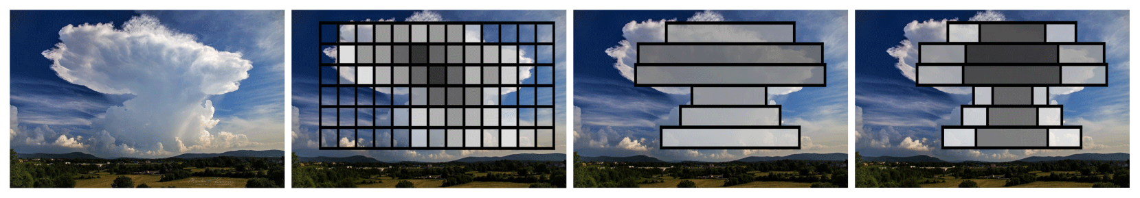
Figure 1First panel: an explosive storm near Divača, Slovenia (Marko Korošec Weather Photography; http://www.markokorosec.net, last access: 12 April 2021). Second panel: a representation of such storm in a cloud-resolving model (lighter/darker gray shading denotes smaller/larger optical thickness). Third panel: a traditional storm representation in coarse-resolution weather and climate models. Fourth panel: the Tripleclouds methodology. Note that the schematics are illustrative and that operational models employ finer vertical resolution.
The present study aspires to make progress on the treatment of cloud–radiation interaction in coarse-resolution weather and climate models, often referred to as the general circulation models (GCMs). Over the past decades, large-eddy simulation (LES) and cloud-resolving models (CRMs) (e.g., Klemp and Wilhelmson, 1978; Tao and Simpson, 1993; Khairoutdinov and Randall, 2003; Stevens et al., 2005) have established themselves as a well-acknowledged tool in cloud physics research (Guichard and Couvreaux, 2017). Short-term global predictions using direct LES/CRM simulations extending up to a few months or even years are beginning to be feasible (Bretherton and Khairoutdinov, 2015). Long-term climate projections utilizing coupled atmosphere–ocean systems in a direct high-resolution mode, however, will not be possible for the next couple of decades even on most powerful supercomputers (Schneider et al., 2017). Similarly, despite remarkable advancements in numerical weather prediction (NWP), which is burdened by the users' demand for real-time forecasts, global NWP at a subkilometer scale will stay challenging in the near future (Bauer et al., 2015).
Bearing the above-mentioned limitations in mind, there remains an ongoing scientific effort to improve traditional physical parameterization schemes, which lie at heart of every weather and climate model. To that end, LES and CRM models provide valuable high-resolution 3-D cloud field data, on which cloud–radiation interplay can be studied either offline (e.g., Jakub and Mayer, 2015; Klinger and Mayer, 2016; Črnivec and Mayer, 2019) or interactively (e.g., Jakub and Mayer, 2017; Klinger et al., 2017; Hartmann et al., 2018). In addition, stochastic cloud models (STMs) allow for quick generation of realistic 3-D cloud structures (e.g., model introduced by Di Giuseppe and Tompkins, 2003a, for stratocumulus; Evans and Wiscombe, 2004, for cumulus; Hogan and Kew, 2005, for cirrus). Whereas the disadvantage of stochastic models compared to LES or CRMs might be that interactive studies of cloud–radiative feedbacks are not possible, our present work is restricted to offline radiation experiments based on cloud data stemming from diverse LES, CRM and STM models.
A number of studies took advantage of this approach in the past. They often compared radiative transfer experiments performed on a pregenerated well-resolved cloud field (Fig. 1, second panel) including the exact 3-D radiation calculation (such as the Monte Carlo technique, Mayer, 2009), the independent column approximation (ICA, Stephens et al., 1991) and the GCM-type radiation calculation. The latter was carried out on the derived horizontally homogeneous cloud representation, where fractional cloudiness was assumed to overlap vertically in accordance with the maximum-random rule (Geleyn and Hollingsworth, 1979) – a configuration which persisted in the majority of GCMs for many decades (Fig. 1, third panel).
In this way, the radiative transfer was extensively studied for cumulus (Davies, 1978; Kobayashi, 1988; Welch and Wielicki, 1989), stratocumulus (Cahalan et al., 1994, 1995; Zuidema and Evans, 1998; Di Giuseppe and Tompkins, 2003a) and cirrus (Carlin et al., 2002; Hogan and Kew, 2005; Zhong et al., 2008; Fauchez et al., 2014), as well as deep convective and anvil clouds (Barker et al., 1999; Fu et al., 2000; Di Giuseppe and Tompkins, 2003b, 2005), although some of the earliest work used either very idealized cuboid, single-layered or 2-D clouds. Moreover, some of these studies assessed solely either the ICA or the subgrid cloud variability error and therefore did not shed any light on their relative contribution. Nevertheless, it was commonly found that classic 3-D radiative effects associated with horizontal photon flow manifest most pronouncedly in areas of notable horizontal gradients of optical properties and are thus regularly related to cloud-side boundaries. But also the in-cloud horizontal variations of optical depth were found to impact 3-D radiative transfer and especially the GCM-type approximation. Due to aforementioned reasons, conflicting claims can be found in the literature regarding the magnitude and sign of these errors. A better understanding of these effects is required to advance the parameterization of cloud–radiation interaction.
1.2 Focus of this study
The present study aims to reinforce earlier studies by establishing 3-D benchmarks and further exploring the validity of ICA for various cloud types. In particular, we intend to assess the ICA suitability when the GCM resolution refines to the mesoscale 𝒪(10–100 km). Di Giuseppe and Tompkins (2003b), as an illustration, showed that 3-D radiative effects increase as the GCM resolution approaches the mesoscale. In addition, we strive to investigate more realistic cloud morphologies, as we applied finer horizontal grid spacing in cloud-generating models compared to the previous research (e.g., Di Giuseppe and Tompkins, 2003b; Hogan and Kew, 2005; Zhong et al., 2008). Furthermore, we aim to consistently analyze atmospheric heating rate and net surface flux, which has received little attention in the previous debates.
The novelty and therefore the prime focus of the current work, however, is the utilization of the Tripleclouds (TC) radiative solver for use in GCMs. While an alternative technique known as the McICA (Pincus et al., 2003) is currently operationally employed in the majority of coarse-resolution models, the TC scheme is attractive because it is free of stochastic noise. The TC method was primarily suggested by Shonk and Hogan (2008) (henceforth abbreviated to SH08) and operates with two regions in each vertical model layer to represent the cloud: one region represents the optically thicker part of layer cloudiness, while the other region represents the remaining optically thinner part. The added value of the Tripleclouds scheme compared to its GCM predecessor using homogeneous cloudiness is thus the capability of accounting for horizontal cloud heterogeneity in the simplest possible and therefore computationally efficient manner. Following the idea of SH08, a second cloudy region has recently been incorporated into the δ-Eddington two-stream method with maximum-random overlap assumption for partial cloudiness by Črnivec and Mayer (2020). The insertion of a second cloudy region in the two-stream framework requires an extension of vertical overlap rules. This task was accomplished by exploiting the core-shell model for convective clouds (Heus and Jonker, 2008; Heiblum et al., 2019), where the convective core characterized by updraft and condensate loading is positioned in the geometrical center of the cloud, enclosed by the shell related to downdrafts and condensate evaporation. In the terminology of radiative transfer, the maximum-random overlap was thus retained for the entire fractional cloudiness and additionally applied for the optically thicker segment. This extended vertical overlap formulation implicitly places the optically thicker cloudy region towards the cloud interior in the horizontal plane, whereas the other optically thinner region covers the cloud periphery, as depicted in Fig. 1 (fourth panel).
In the study by Črnivec and Mayer (2020), the TC scheme was at first evaluated on a broken shallow cumulus, where it proved to be a significant improvement compared to the GCM approach on homogeneous clouds. Herein, we extend the work of Črnivec and Mayer (2020) by examining additional case studies of stratocumulus, cirrus and cumulonimbus, since cloud horizontal heterogeneity strongly depends on cloud type (Pincus et al., 1999; Oreopoulos and Cahalan, 2005; Shonk et al., 2010; Shonk and Hogan, 2010; Boutle et al., 2014; Hill et al., 2012, 2015). These case studies were deliberately chosen in such a way that cloud vertical arrangement tends towards the assumed maximally overlapped scenario. This enables us to focus on radiative effects associated with cloud horizontal inhomogeneity, while eliminating the error arising from the misrepresentation of assumed vertical overlap as would be expected to occur in conditions with strong vertical wind shear (Naud et al., 2008; Di Giuseppe and Tompkins, 2015).
Once two-stream radiative fluxes have been imposed onto a system of three-region atmospheric layers, the research challenge is to optimally set the pair of liquid ice water content (LWC IWC) characterizing the two cloudy regions and the corresponding geometrical split of layer cloudiness. The answer to the posed scientific question is critically dependent on the characteristic of the subgrid cloud horizontal variability. The latter is conveniently defined by the fractional standard deviation (FSD) of cloud condensate as well as the shape of condensate distribution. The parameter FSD (e.g., of LWC) is defined as the standard deviation (σLWC) divided by the mean (), whereby only the non-zero values in the horizontal LWC distribution are considered. Since this information is generally not available in GCMs, Shonk et al. (2010) estimated a global FSD based upon diverse cloud observational studies. The prime objective of the present study is to assess the validity of the global FSD estimate in the TC radiative solver for three inherently contrasting cloud types in conjunction with various assumptions for condensate distribution, which are commonly applied in cloud modeling (Gaussian, gamma, lognormal). Along the above lines, a further goal of the study is to inspect the actual cloud condensate distribution based on high-resolution LES/CRM data, as this is the keystone for a well-designed self-consistent TC parameterization. The majority of previous studies examining cloud condensate distribution adopted cloud data simulated on smaller domains with coarser grid spacing. The final aim of the study is to explore more sophisticated FSD parameterizations, characterizing systematic departures from the global mean. These refined TC configurations refer to distinctive improvements for overcast and extremely heterogeneous cloudiness. Together with the parent study of Črnivec and Mayer (2020), this work presents the first usage of Tripleclouds to consistently study the cloud-layer heating rate and net surface flux.
The remainder of this paper is structured as follows: the cloud data and methodology are presented in Sect. 2. The results of the radiative transfer experiments are discussed in Sect. 3. Section 4 concludes with a brief summary and outlook.
2.1 Cloud field data
Input data for radiative transfer experiments is a set of 3-D highly resolved inhomogeneous cloud fields, defined in terms of LWC and IWC distributions. These differing cloud cases comprise a wide range of inhomogeneity observed in nature. In the following, each cloud type is characterized briefly.
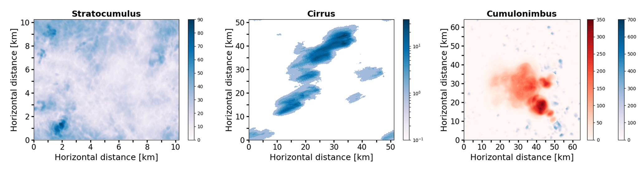
Figure 2Vertically integrated visible optical thickness of selected cloud field case studies. Note that in the case of cumulonimbus, the blue/red shading denotes optical thickness of liquid/ice water content.
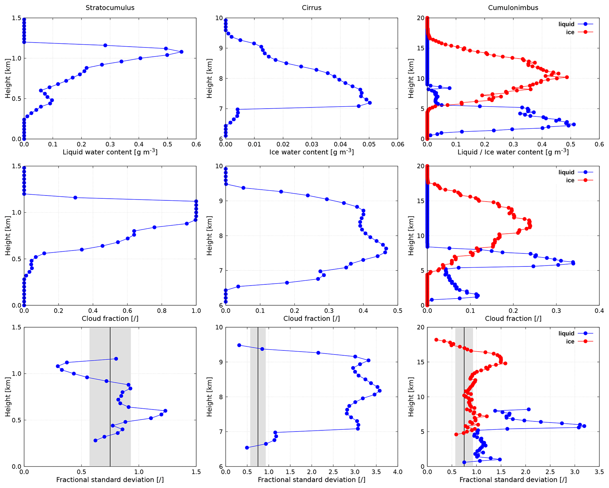
Figure 3Characterization of selected cloud field case studies in terms of averaged LWC IWC (top row), cloud fraction (middle row) and fractional standard deviation of LWC IWC (bottom row), whereby the vertical black line shows the mean global FSD estimate and the gray-shaded area denotes its uncertainty (Shonk et al., 2010).
2.1.1 Stratocumulus
The stratocumulus was simulated with the University of California, Los Angeles large-eddy simulation (UCLA-LES) model (Stevens et al., 2005). The simulation relates to the Atlantic Stratocumulus Transition Experiment (ASTEX; Albrecht et al., 1995), conducted over the northeast Atlantic Ocean in June 1992. The case study thereby exemplifies a marine boundary layer stratocumulus, exhibiting sporadic convective cells embedded in the stratus layer (Agee et al., 1973; Atkinson and Zhang, 1996; Wood and Hartmann, 2006). Observational studies show that directional and magnitude vertical shear is small in mesoscale cellular convection (Agee et al., 1973). The horizontal domain size is 10.24×10.24 km2, with the vertical extent of the domain being 4 km. A constant model grid spacing of 40 m is applied in all three (x, y, z) directions. Figure 2 (left) visualizes the cloud field in terms of vertically integrated optical thickness. Vertical profiles of averaged LWC, cloud fraction (defined by LWC > 10−3 g m−3) and FSD are shown in Fig. 3 (left). The overcast stratocumulus scene is topped slightly above 1 km height. The FSD, although roughly centered around the global estimate, strongly depends on the position within the cloud layer: it exhibits a maximum (1.2) in the lowest portion of the cloud layer and a minimum (0.3) in its uppermost radiatively important region.
To gain further insight about the subgrid cloud variability, the theoretical distributions (Gaussian, gamma, lognormal) were fitted to the actual LWC distribution in each vertical layer, so that they had the same mean and standard deviation as the actual data. The goodness of fit was assessed with the Kolmogorov–Smirnov test. The investigation revealed that the actual LWC distribution throughout the majority of the upper portion of the cloud, where radiative effect is maximal, is best approximated with the lognormal distribution (best fit in five-eighths of the top layers), followed by the gamma distribution which performs similarly well.
2.1.2 Cirrus
The cirrus was generated with the stochastic cloud model (Cloudgen) of Hogan and Kew (2005), described also in Zhong et al. (2008). The speciality of this 3-D cirrus fractal model is its capability to generate structural features unique to cirrus clouds: realistic fallstreak geometry and shear-induced mixing. The model input parameters are based on the statistics derived from radar observations in southern England (Hogan et al., 2003; Hogan and Illingworth, 2003). We chose the cirrus uncinus case study of 24 June 1999, which is the first of the three cases discussed by Hogan and Kew (2005) and subsequently also by Zhong et al. (2008)1 and was adopted herein as it is the case with smallest vertical wind shear. The horizontal domain size is 51.2×51.2 km2 with a grid spacing of 100 m. The vertical extent of the domain is 7 km using constant vertical grid spacing of 109 m. Figure 2 (middle) visualizes the cloud field in terms of vertically integrated optical thickness. Vertical profiles of averaged IWC, cloud fraction (defined by IWC > 10−3 g m−3) and FSD are shown in Fig. 3 (middle). The degree of cloud horizontal heterogeneity is largest in the central part of the cloud layer, with FSD exceeding 3.5. The cirrus layer is thus by far not uniform; rather, it exhibits cellular structures (“generating cells”), which would in reality be associated with convective motions. The latter produce higher supersaturations (Heymsfield, 1977) and increase cirrus ice crystal residence time (Mitchell, 1994), which leads to an increased IWC within the cells. The layer IWC of the present cirrus is lognormally distributed, as this is the intrinsic Cloudgen property.
2.1.3 Cumulonimbus
The cumulonimbus was simulated with the Goddard Cumulus Ensemble cloud-resolving model (GCE-CRM), described in detail by Tao and Simpson (1993) and more recently by Tao et al. (2003). The simulation relates to the convective event observed on 23 February 1999 during the Tropical Rainfall Measuring Mission (Simpson et al., 1988, 1996) Large-Scale Biosphere-Atmosphere (TRMM-LBA) experiment in the Amazon. The horizontal domain size is 64.0×64.0 km2, with the vertical extent of the domain being 23 km, which is sufficient to allow the growth of tropical cirrus anvil. A grid spacing of 250 m is applied in each horizontal direction and 200 m in the vertical direction. The simulation is described by Lang et al. (2007) and briefly by Zinner et al. (2008). Due to light environmental winds (Fig. 2b of Lang et al., 2007), the convection was rather weakly organized.2 Figure 2 (right) visualizes the cloud field in terms of vertically integrated optical thickness. Vertical profiles of averaged LWC and IWC, the corresponding cloud fraction, as well as FSD are shown in Fig. 3 (right). The case study is characterized by three distinct cloud layers: a liquid-phase region extending from 0.8 to 4.4 km consisting of shallow cumuli, a mixed-phase stratiform region located between 4.4 and 8.2 km, and an ice-phase region extending from 8.2 to 17.4 km height, encompassing the cumulonimbus deep convective core and the anvil. Remarkably, the stratiform layer is highly heterogeneous, with the maximum FSD of the liquid phase exceeding 3.2. The maximum FSD in the bottommost cumuliform region as well as in the uppermost anvil region reaches approximately half of this value.
The comparison of theoretical distributions with actual LWC IWC distributions reveals the following findings: the assumption of Gaussianity is void for the present cumulonimbus scenario and in each vertical layer either gamma or lognormal distribution was classified as the best fit. Thus, throughout the majority of the liquid region, the actual LWC distribution is best approximated with the gamma distribution (best fit in 58 % of layers). In the mixed-phase region, the LWC distribution is best approximated with the lognormal distribution (best fit in 85 % of layers), whereas the IWC distribution is best approximated with the gamma distribution (best fit in 85 % of layers). In the ice region, the IWC distribution is best approximated with the gamma distribution within the bottommost 30 % and uppermost 13 % of the region (best fit in all cases), while within the remaining central part the lognormal distribution appears to be the optimal approximation (best fit in 58 % of layers).
2.2 Configuring Tripleclouds experiments
2.2.1 Baseline Tripleclouds experiments
To utilize the TC radiative solver, a pair of LWC IWC values defining the two cloudy regions has to be generated in each vertical layer. We refer solely to the liquid phase in the remainder of this section, since analogous considerations apply to the ice phase. Thus, the LWC values characterizing the optically thin and thick cloudy region are referred to as the LWCcn (Cloud thiN) and LWCck (Cloud thicK). Based on the analysis of high-resolution cloud radar data, SH08 showed that TC performs well for top-of-the-atmosphere (TOA) radiative fluxes when the LWCcn is chosen to be the value corresponding to the 16th percentile of the observed LWC distribution, whereas the LWCck is determined under conservation constraints of the in-cloud mean LWC (denoted as ):
This method is referred to as the “lower percentile (LP) method” and utilizes a “split percentile (SP)” of 50, implying that cloudiness in each vertical layer is divided through a median of distribution into two equal parts.
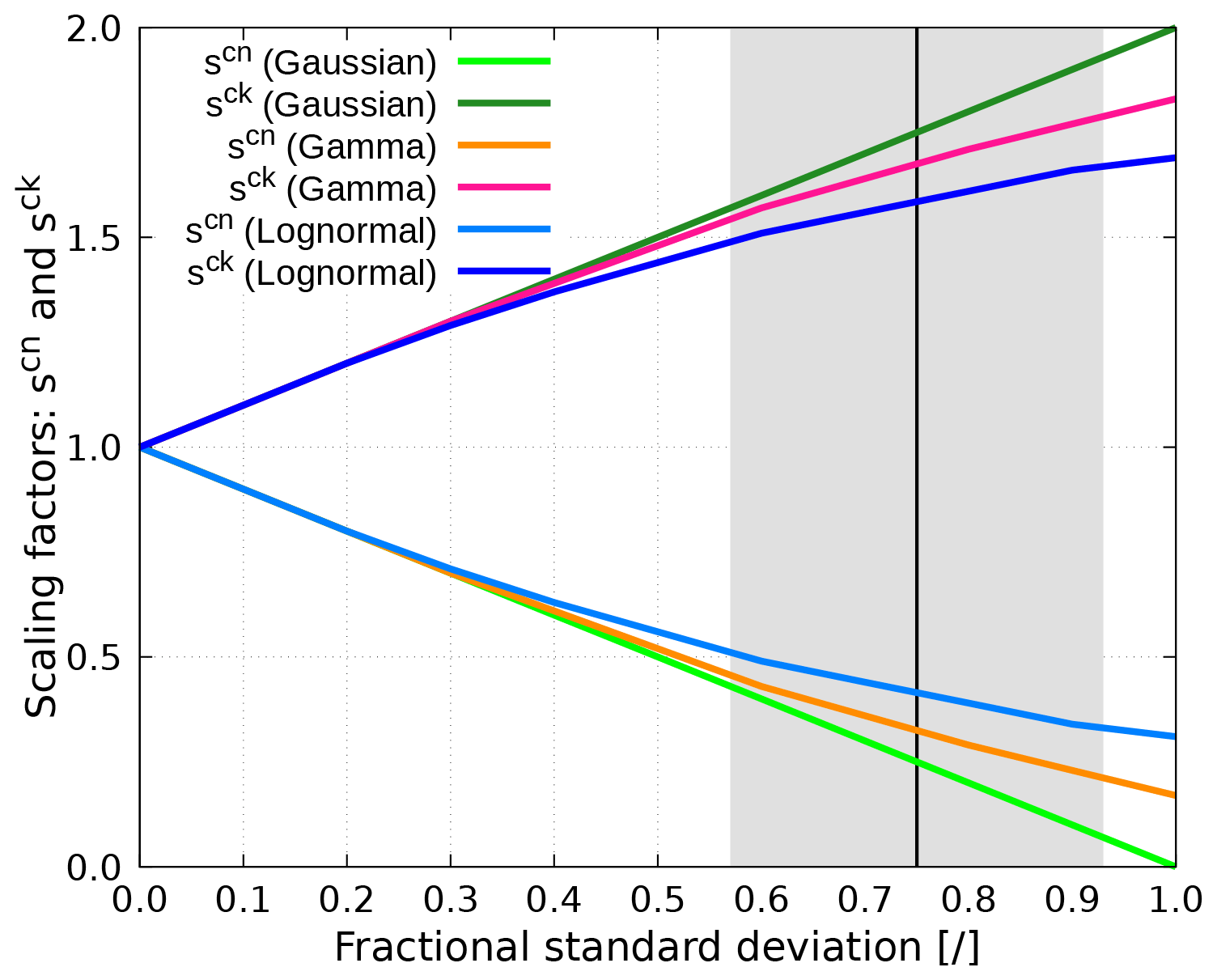
Figure 4Scaling factors (scn, sck) of for Gaussian, gamma and lognormal distributions. The black line and the gray area represent mean global FSD and its uncertainty.
When the TC solver resides in a host GCM model, however, the details about the underlying LWC variability are not known; therefore, several assumptions have to be introduced. To obtain the pair (LWCcn, LWCck) from , which is indeed available in a GCM, we introduce the so-called -scaling factors for the optically thin and thick cloudy regions. These are termed scn and sck and fulfill the following relationships:
Different parameters to define the degree of cloud horizontal inhomogeneity are employed in the existing literature and numerical models (e.g., Cahalan et al., 1994; Smith and Del Genio, 2001; Carlin et al., 2002; Rossow et al., 2002; Oreopoulos and Cahalan, 2005). A frequently used parameter is the previously introduced fractional standard deviation of LWC. The FSD is a convenient measure, since it accounts for a strong correlation between and σLWC (Smith and Del Genio, 2001; Carlin et al., 2002; Hill et al., 2012). Based on a comprehensive review of numerous observational studies encompassing diverse cloud data sets, Shonk et al. (2010) converted various variability measures into a single globally applicable FSD parameter. Its mean value and uncertainty are
When TC is employed in a host GCM, moreover, an assumption about the shape of LWC distribution has to be made. To this end, we test three assumptions for subgrid cloud condensate distribution: Gaussian distribution, which traditionally prevailed in many models due to its simplicity, as well as more realistic gamma (supported by Barker et al., 1996; Pincus et al., 1999; Carlin et al., 2002; Rossow et al., 2002) and lognormal distribution (supported by Pincus et al., 1999; Hogan and Illingworth, 2003). For a Gaussian distribution, the 16th percentile (suggested by SH08) is given by
although caution needs to be taken as this expression becomes unphysical for FSD > 1. Similarly, according to Hogan et al. (2019), for a gamma distribution, the 16th percentile is approximated by
Finally, according to Hogan et al. (2016), for a lognormal distribution,
For any FSD value, the scn defined with Eq. (6) or (7) lies in the range between 0 and 1. The desired conservation of implies , where the layer cloudiness is geometrically halved. The approach outlined above, utilizing any of the selected distributional assumptions to generate the LWC pair, is referred to as the “FSD method” in the remainder of this paper. The resulting -scaling factors for Gaussian, gamma and lognormal distributions as a function of FSD are shown in Fig. 4. It is apparent that in the region of the global FSD estimate, the pair (LWCcn, LWCck) exhibits a large sensitivity to the assumed form of LWC distribution. This signifies the meaningfulness to pose a question, whether different condensate distribution assumptions significantly affect radiative quantities when global FSD is applied as a proxy for cloud internal variability.
In order to verify (or discard) the validity of the global FSD estimate for heating rates and surface fluxes, we applied its mean value of 0.75 (abbreviated to “G”) in the baseline TC(FSD) experiments together with all three distributional assumptions. In addition to the baseline calculations performed on each cloud type, we aimed to explore more advanced TC configurations, specifically targeting to optimize the treatment of the overcast stratocumulus and highly heterogeneous cirrus. The optimization methodology is described in the following.
2.2.2 Optimization for overcast cloud scenarios
It was previously pointed out that in the uppermost radiatively important overcast part of the stratocumulus, the actual FSD is smaller than the introduced global estimate. This might be partially attributed to the fact that overcast grid boxes do not contain cloud edges, which generally contribute to increased variability. Mixing of cloudy and cloud-free air at the edges of clouds, namely, tends to decrease the mean LWC as well as increase the spread of LWC, both acting to increase the FSD. A grid box excluding cloud edges will therefore have lower FSD. To that end, we test the parametric FSD relationship for liquid cloud inhomogeneity proposed by Boutle et al. (2014), denoted as B14, developed based on a rich combination of satellite, in situ and ground-based observations. This parameterization takes into account that variability is generally dependent on grid box horizontal size (x [km]) and cloud fraction (C). It exhibits a discontinuity at C=1 capturing the aforementioned cloud edge effect:
where
The optimized TC experiment using the FSD parametrization of B14 assumes the LWC is lognormally distributed.
2.2.3 Optimization for highly heterogeneous cloud scenarios
The key point worth mentioning when highly heterogeneous scenes such as the cirrus are tackled with the TC solver is that the split percentile of 50 (geometrically halving layer cloudiness when allocating optically thin and thick portions of the cloud) is not the best choice (Hogan et al., 2019). The examination of IWC distribution in each vertical layer of the present cirrus indeed reveals that these are highly skewed (with a modal value close to zero and a long tail with rarely occurring high IWC). Therefore, it seems reasonable to allocate a larger portion of the cloud to the optically thinner region. This concurrently implies increasing the weighting of IWCcn and decreasing the weighting of IWCck, whereby the latter is shifted to a higher value to conserve the layer mean. In order to discern the optimum geometrical partitioning of the cirrus into two parts, we carried out multiple experiments with global FSD, gradually increasing the SP from 50 to 99 (the limit of 100 coincides with the horizontally homogeneous cloud representation). Further, we aimed to evaluate the parameterization for ice cloud inhomogeneity of Hill et al. (2015), denoted as H15, developed on the basis of CloudSat (Stephens et al., 2002, 2008) data products. All optimized TC experiments model the subgrid IWC distribution as lognormal.
2.3 Setup of radiative transfer calculations
The radiative transfer simulations were carried out with the libRadtran software (Emde et al., 2016). For consistency, the calculation setup is the same as in Črnivec and Mayer (2020). Here, we summarize basic parameter settings and provide additional information regarding the treatment of the ice phase, which was absent in our preceding study. Thus, except for 3-D fields of LWC and IWC as well as the assigned effective radii (parameterized following Bugliaro et al., 2011), all atmospheric conditions are assumed to be horizontally homogeneous and correspond to the US standard atmosphere (Anderson et al., 1986). The domain extends vertically up to a height of 120 km, which is considered to be the TOA. In the lowest portion of the domain where clouds are located, we preserved the original high-resolution vertical grid as inherited from the parent cloud model and interpolated the background standard atmospheric conditions onto this grid. It should be reminded that solely LWC and IWC were used as input for radiation calculations to define the cloud fields, while other hydrometeor categories (i.e., precipitation-sized particles, such as rain, snow and graupel) were excluded from the analysis. Optical properties of water droplets (assumed to be spherical) were prescribed following the parameterization of Hu and Stamnes (1993). Optical properties of ice crystals were specified based on the parameterization of Yang et al. (2000), assuming habit of hexagonal columns. Solar zenith angle (SZA) was varied between 0∘ (overhead Sun), 30∘ and 60∘, whereby downward flux at TOA corresponds to 1365, 1182 and 683 W m−2. At the surface, the temperature of 288.2 K implies upward flux of 389.5 W m−2 according to the Stefan–Boltzmann law. The surface was assumed to have a constant albedo of 0.25 in the solar spectral range, whereas in the thermal spectral range it was assumed to be black (albedo of 0).
Table 1 summarizes the radiation experiments carried out in this study. The benchmark experiment was performed using the 3-D Monte Carlo radiative model MYSTIC (Mayer, 2009). The horizontal extent of the domain matched that of each individual cloud field case study. Periodic boundary conditions were applied in the 3-D configuration. In addition, the Monte Carlo experiment in ICA mode was carried out, which is the same as the 3-D experiment, except that periodic boundary conditions are imposed at each grid column. The 3-D and ICA experiment were both performed on the high-resolution cloud grid, with the result subsequently horizontally averaged across the domain. The difference between the ICA and 3-D results was used to assess the impact of horizontal photon transport on domain-averaged (GCM-scale) radiative quantities. Whereas the exact number of traced photons depends on the particular cloud case, it was held sufficiently high, so that the Monte Carlo noise of domain-averaged quantities was kept below 0.1 %. Moreover, we performed a GCM-type calculation on a layer-averaged fractional cloud using the δ-Eddington two-stream method with maximum-random overlap assumption for partial cloudiness, which was recently implemented into libRadtran (Črnivec and Mayer, 2019). The Tripleclouds solver was employed in conjunction with the LP method based on the observed condensate distribution and the FSD method utilizing the distribution assumption in various configurations as outlined in Sect. 2.2.

For each experiment, we diagnosed atmospheric heating rate and net surface flux in the solar and thermal part of the spectrum, as well as their total (integrated) effect. The error is measured by the absolute error (Eq. 9) and relative error (Eq. 10) and for the heating rate profile additionally by the cloud-layer RMSE (Eq. 11):
where x represents the 3-D benchmark and y represents the outcome of either the ICA, GCM or any TC experiment. The cloud-layer RMSE denotes the RMSE evaluated throughout the vertical extent of the cloud layer of each particular cloud field case study.
We discuss the atmospheric heating rate and net surface flux for each cloud type. The results of the 3-D, ICA, GCM and baseline TC experiments are presented first, whereas subsequently the optimized TC experiments are highlighted.
3.1 Stratocumulus
3.1.1 Atmospheric heating rate
Figure 5 (top row) shows the radiative heating rate in the benchmark 3-D experiment for the stratocumulus cloud. There is large absorption of solar radiation in the cloud layer, resulting in the maximum heating rate of about 53, 47 and 27 K d−1 at SZA of 0, 30 and 60∘, respectively. The peak heating rates are concentrated in the uppermost part of the cloud layer, since both cloud fraction and LWC increase from cloud base towards cloud top. In the thermal spectral range, the cloud layer is subjected to strong cooling, reaching a peak of almost −140 K d−1 at the same height where maximum solar heating is attained. These large heating and cooling rates are partially a manifestation of high vertical resolution (Di Giuseppe and Tompkins, 2003a). The total heating rate, a physically relevant quantity during daytime, is dominated by thermal cooling. This persistent cloud-top radiative cooling is a typical feature of marine stratocumulus-topped boundary layers (STBLs; Wood, 2012). It drives convective instability and controls turbulence within the underlying mixed layer (Randall, 1980; Deardorff, 1981; Stevens et al., 1999), when adequately coupled to a dynamical model. The radiative errors could therefore importantly affect the evolution of the stratocumulus layer itself.
The examination of radiative errors (Fig. 5, bottom row) reveals that these are maximized in the uppermost part of the stratocumulus layer as well. The disparity between the ICA and 3-D is minor: a maximum difference of −0.2 K d−1 is observed in the solar spectral range for SZA of 60∘ (cloud-side illumination effect; Jakub and Mayer, 2015, 2016). In the thermal spectral range, the ICA underestimates the amount of 3-D cooling by about 2.5 K d−1 in the uppermost grid point of the cloud layer (cloud-side cooling effect; Klinger and Mayer, 2014, 2016). These comparatively small ICA errors are attributed to the minor cloud-top topography (difference between the nearby local height maximum and minimum; Zuidema and Evans, 1998) of the present stratocumulus. The radiative transfer, namely, acts to smooth out structures at spatial scales smaller than the photon mean free path, with the latter corresponding to several hundred meters in STBLs (Marshak et al., 1995).
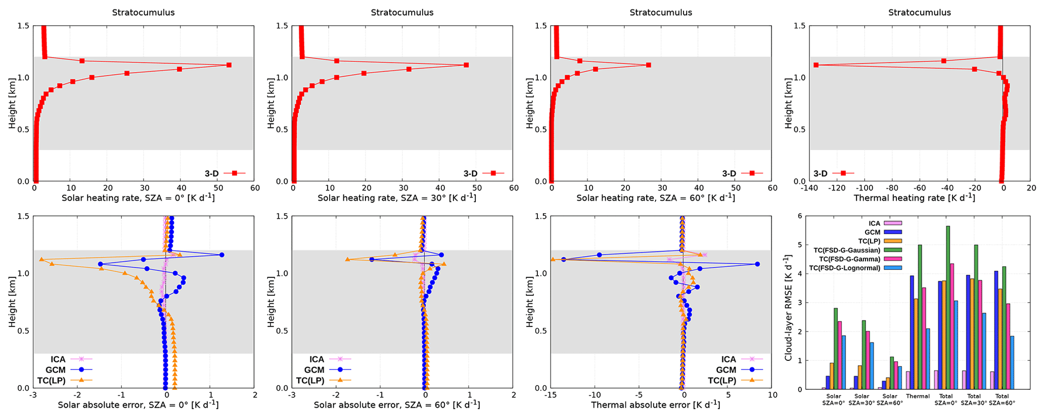
Figure 5Radiative heating rate for the stratocumulus cloud. The gray-shaded area denotes the cloud layer.
The GCM error exhibits a pronounced vertical gradient within the cloud layer: in the uppermost part of the cloud layer, the GCM solar heating rate is too high, while in the region underneath it is too low (at all SZAs). In the thermal spectral range, the opposite is the case, but the error is quantitatively larger and dominates the daytime error. Thus, the GCM boosts radiatively driven destabilization of the stratocumulus layer during daytime and nighttime. It overestimates cooling in the uppermost region of the layer by −14 K d−1 and it overestimates warming in the region underneath by up to 9 K d−1. The physical explanation for the GCM bias arising from homogeneous cloudiness is given by Črnivec and Mayer (2020).
In the baseline Tripleclouds experiments, the solar error is increased compared to that of the GCM. This is most notable when using the FSD method, since the global FSD introduces excessive heterogeneity in the radiatively important upper part of the cloud layer. In the thermal spectral range, the TC in most configurations outperforms the GCM. Further, the TC appears to be strongly sensitive to the assumed condensate distribution, highlighting its importance, with the lognormality assumption performing best. It is worth noting that, although the TC with global FSD degrades the solar error, it is still more accurate than the GCM during all nighttime and daytime conditions, when LWC lognormality is assumed. In particular, nocturnal cloud-layer RMSE is reduced from about 3.9 K d−1 to only 2.1 K d−1. The largest daytime improvement is observed at SZA of 60∘, where RMSE is reduced from 4.1 K d−1 to solely 1.8 K d−1.
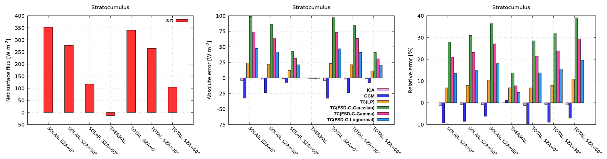
Net surface flux
Figure 6 shows the net surface flux underneath the stratocumulus. The ICA error is small during daytime and nighttime, maximized at overhead Sun (up to −5 W m−2 or −2 %). This is essentially attributed to the photon cloud-side escape effect (Várnai and Davies, 1999), where preferential forward scattering on cloud droplets increases 3-D surface downward radiation (Wissmeier et al., 2013). An increased solar absorption in the homogeneous GCM cloudiness implies reduced transmittance and hence underestimated daytime net surface flux. The error is largest at overhead Sun (−33 W m−2 or −9 %) and decreases with increasing SZA, whereas at nighttime the GCM error is minor.
When the TC(LP) is applied, the net flux error is mostly slightly reduced, whereas in TC(FSD) baseline experiments the error is increased compared to the GCM. The latter finding is consistent with previous considerations, where it was pointed out that global FSD introduces excessive inhomogeneity to the radiatively important part of the stratocumulus, unrealistically reducing the absorption of solar radiation within the cloud layer. The corresponding increased cloud-layer transmittance, as we demonstrated herein, has important implications for the surface budget; therefore, proposed optimization is highlighted in the next section.
It should finally be noted that also the assumed maximum overlap of optically thicker cloudy regions could result in a somewhat excessive transmission towards the surface (compared to the situation in a GCM). The vertical decorrelation length of in-cloud heterogeneities is typically assumed to be half that of cloud boundaries (Shonk et al., 2010). If this phenomenon was implemented in the TC scheme, it would block more of the solar radiation and reduce the positive surface net flux error.
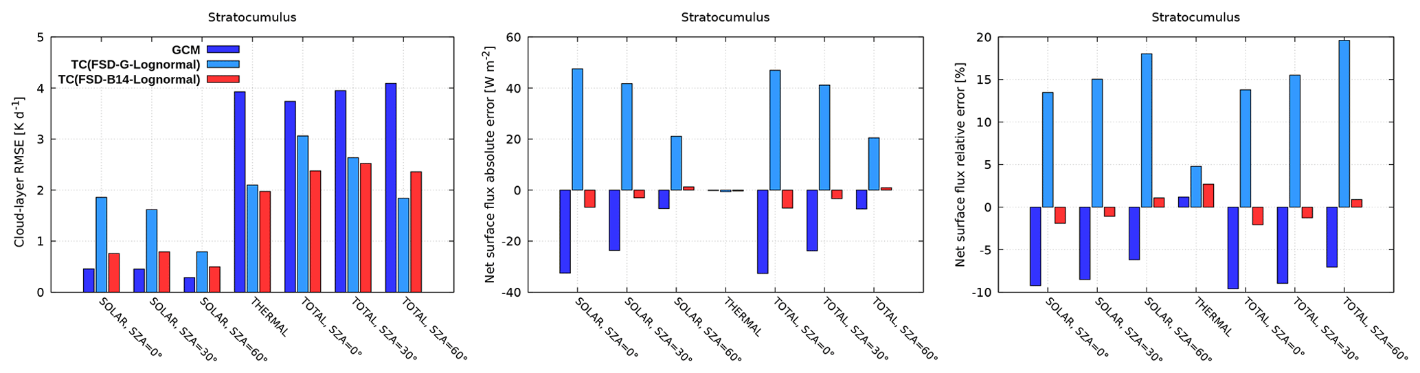
3.1.2 Optimization for overcast cloud scenarios
Figure 7 shows the results of the GCM calculation, the Tripleclouds in its baseline lognormal configuration with the global FSD estimate as well as the corresponding refined TC experimentation where the FSD within the stratocumulus layer is parameterized according to B14. The nighttime and daytime cloud-layer RMSE (Fig. 7, left) in the refined TC experiment is generally slightly reduced (except at low Sun) compared to its counterpart in the baseline configuration and remains considerably lower than that in the GCM for all nighttime/daytime conditions. Most importantly, the net surface flux error (Fig. 7, middle and right), which in the baseline TC setup was even larger than in the GCM experiment, is significantly reduced in the refined Tripleclouds venture.
3.2 Cirrus
Figure 8 (top row) shows the radiative heating rate in the benchmark 3-D experiment for the cirrus cloud. The solar absorption in the ice layer results in a maximum heating rate of about 3.6, 3.3 and 2.2 K d−1 at SZA of 0, 30 and 60∘, respectively. The height where this maximum heating is reached stays the same for all SZAs and corresponds to the height of maximum cloud fraction (7.6 km). In the thermal spectral range, a peak cooling of −2.9 K d−1 is attained higher up in the cloud layer (at 8.7 km; effective cloud top; above this height cloud fraction rapidly decreases), followed by a peak warming of 1.5 K d−1 located at the height of maximum IWC (7.1 km; effective cloud base; below this height, IWC is sharply reduced). In contrast to the stratocumulus, solar heating and thermal cooling observed on the cirrus are more evenly distributed throughout the cloud layer, whereas thermal warming remains confined to a shallow region at cloud base. The daytime heating rate is governed by the stronger thermal effect, although solar heating largely compensates thermal cooling. Compared to the stratocumulus, the heating rate on the cirrus is overall much lower. Nevertheless, it should be kept in mind that the net heating rate in the upper troposphere and lower stratosphere (UTLS) is close to zero (Haigh, 1984), which makes this region highly sensitive to small radiative errors.
The 3-D solar effects (Fig. 8, bottom row) are present at all SZAs and maximized at 60∘ (cloud-side illumination), where the ICA error of −0.1 K d−1 is observed throughout the majority of the cloud layer. In the thermal spectral range, the ICA error is negligible. Similar results were found by Zhong et al. (2008) (recall that the latter investigated the same midlatitude cirrus, although on a coarser grid), who also showed that domain-averaged ICA and 3-D heating rates agree within 0.1 K d−1 in both the longwave and the shortwave.
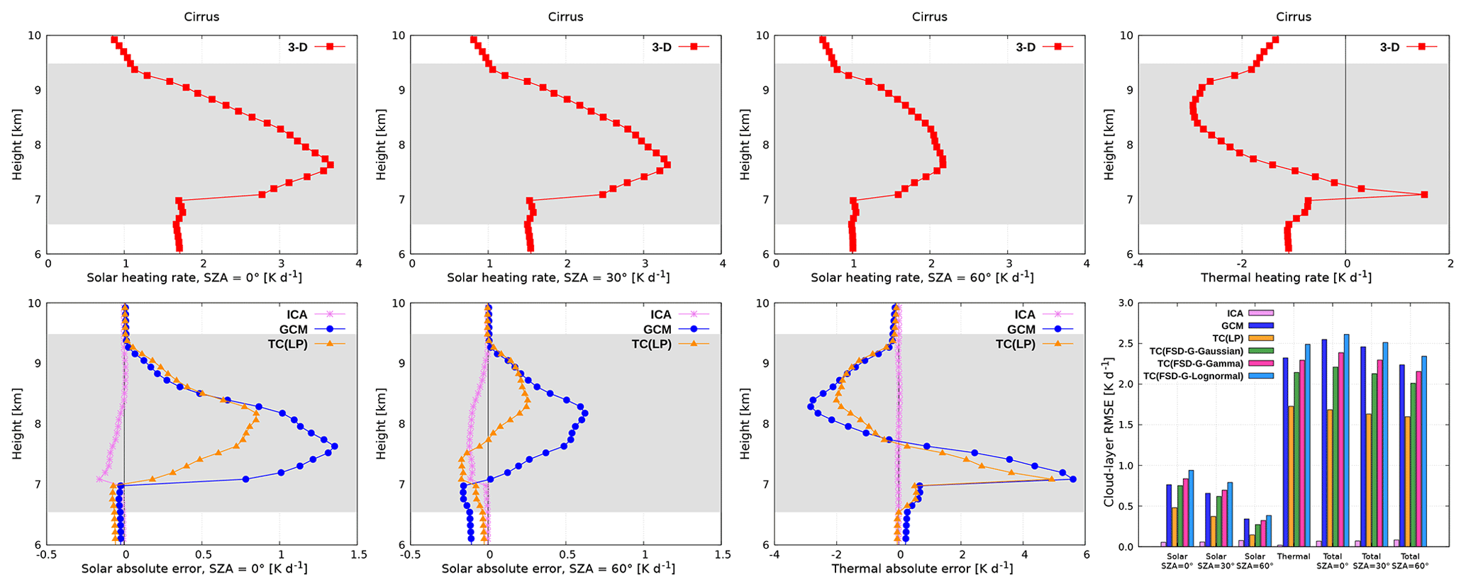
Figure 8Radiative heating rate for the cirrus cloud. The gray-shaded area denotes the cloud layer.
In the GCM, the solar heating rate is overestimated by up to 1.4, 1.2 and 0.7 K d−1 at SZA of 0, 30 and 60∘, respectively. The height where this maximum error is observed corresponds to the height of maximum benchmark heating. In the thermal spectral range, the GCM error enhances radiatively driven destabilization of the cirrus layer by an overestimation of top cooling by 2.8 K d−1 and a substantial overestimation of base warming (error exceeding 5.6 K d−1). The thermal GCM error is in close agreement with that observed by Zhong et al. (2008), whereas the solar GCM error is by a factor of 2 to 3 smaller. The latter finding indicates the potential dependence of GCM errors on the initial cloud grid resolution, which could affect the TC experiments as well and has to be more thoroughly examined in the future. The daytime GCM error profile closely resembles that of its nighttime counterpart, such that the radiatively driven destabilization of the cirrus layer is persistently substantially escalated.
Among the baseline Tripleclouds experiments, the TC(LP) performs best, reducing the GCM error in the solar, thermal and total spectral range at all SZAs. Despite the fact that the actual IWC is lognormally distributed, the TC(FSD) performs best with the Gaussianity assumption. The latter implies the largest difference between the IWC pair defining the two cloudy regions (Fig. 4), partially accounting for the missing inhomogeneity provided by global FSD.

3.2.1 Net surface flux
Figure 9 shows the net surface flux underneath the cirrus. The ICA underestimates the 3-D benchmark, primarily due to the aforementioned cloud-side escape, although this phenomenon is less noticeable for optically thin cirrus (error held below −3 W m−2 or −1 %). The GCM, on the contrary, reveals large errors. Whereas the absolute error is largest at high Sun (−33 W m−2 at SZA of 0 and 30∘ during daytime), the relative error is maximized at SZA of 60∘ on account of a strongly reduced benchmark. Insufficient surface nighttime cooling in the GCM implies an error of 5.5 W m−2 (−6 %).
All Tripleclouds baseline experiments perform better than the GCM. The largest amelioration is observed at nighttime, where the TC(LP) practically depletes the entire error, while TC(FSD) experiments generally halve the GCM error. Nevertheless, alternative arrangements for better TC utilization are investigated next.
3.2.2 Optimization for highly heterogeneous cloud scenarios
Figure 10 (top row) shows the cloud-layer RMSE and net surface flux error using TC with different FSD parameterizations (global estimate, H15) for three selected splitting events. The latter are characterized by the SP of 50 (baseline), 75 and 90 (allocating three-fourths and nine-tenths of layer cloudiness to the optically thinner region). For comparison, the GCM experiment is shown as well. It is apparent that there is a considerable sensitivity to the choice of geometrical splitting, with the most asymmetrical split (matching the SP of 90) performing best in all cases. It is worth noting that, at a given splitting event, the experiments where the FSD is parameterized according to H15 mostly lead to degraded results compared to those with global FSD (in particular at best-split scenario with SP of 90). Thus, although the parameterization of H15 incorporates height dependence of horizontal variability (via cloud fraction), it underestimates the actual FSD being even smaller than the global estimate (Fig. 10, middle row, left), which brings the aforementioned radiative degradation. Further research oriented towards advanced retrievals of high cloud inhomogeneity is therefore firmly advocated. Vertical profiles of solar and thermal heating rate in TC experiments with global FSD for the aforementioned splitting events are further compared with the GCM in Fig. 10. For highly asymmetrical splitting, the cloud–radiative error throughout the majority of the cirrus layer is significantly reduced.
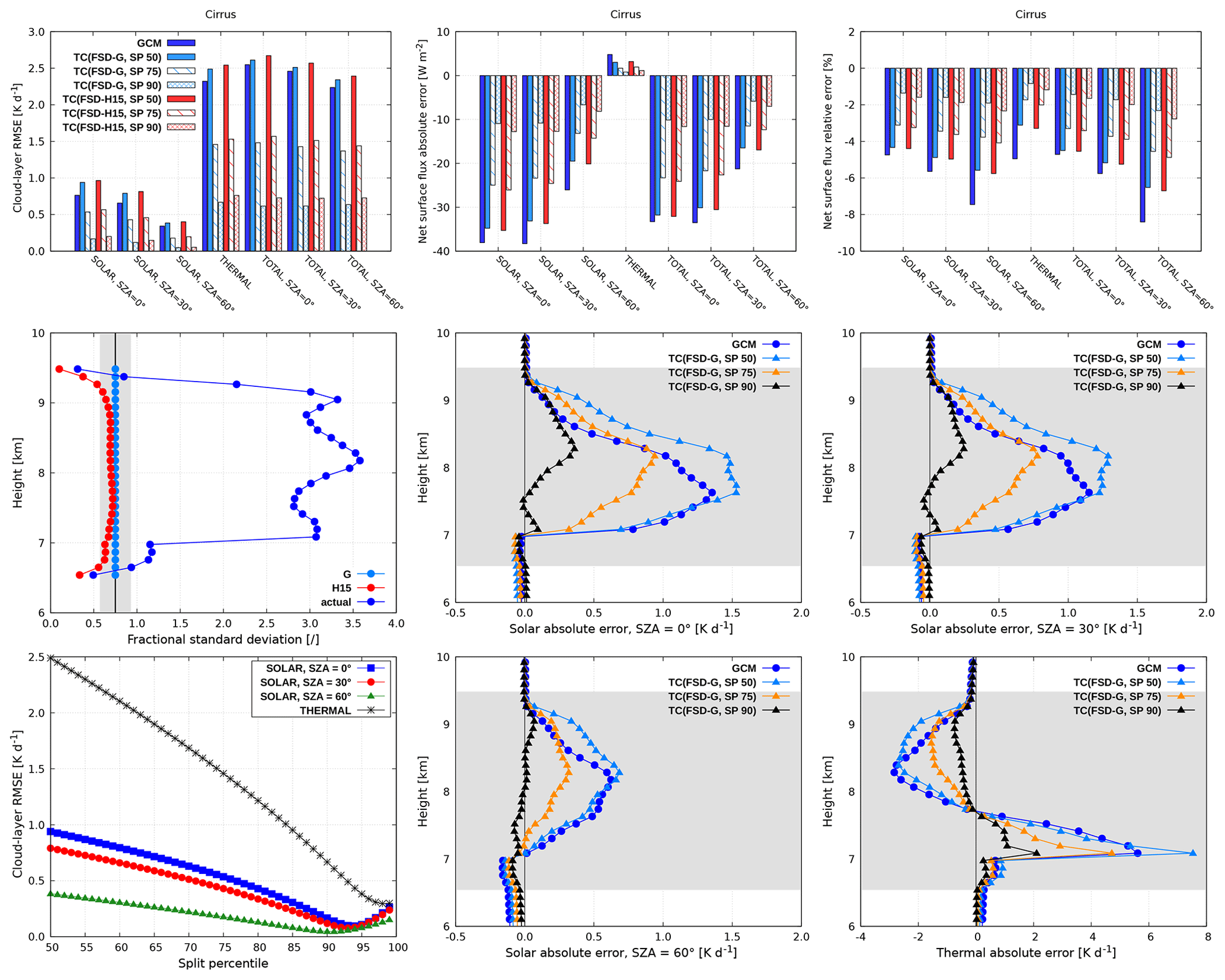
Figure 10Optimizations for cirrus (subgrid variability is modeled lognormally in all TC experiments shown).
Figure 10 (bottom left) shows the cloud-layer RMSE of TC experiments with global FSD for the entire range of splitting events. In the solar part of the spectrum, the optimum SP minimizing the error indeed lies around 90 (the exact value depends on SZA). Increasing the SP beyond this optimum value degrades the heating rate in the cirrus layer. In the thermal part, on the contrary, the RMSE practically monotonically decreases as the SP is increased. Hence, the thermal RMSE exhibits a minimum when the TC is configured so that the entire layer cloudiness is attributed to the optically thinner region (horizontally homogeneous cloud representation with an effective IWC equal to IWCcn). This indicates that for extremely heterogeneous scenes, such as the present cirrus, the radiation scheme employed in a weather or climate model could alternate between the Tripleclouds in the solar spectral range and the computationally more efficient GCM solver using homogeneous clouds in the thermal spectral range, albeit with scaled IWC (effectively the traditional scaling factor method). Finally, in more detailed future studies additionally considering vertical overlap issues, it should be kept in mind that the fixing of cloud horizontal inhomogeneity and vertical overlap should be addressed concurrently to avoid the problem of compensating errors (Shonk and Hogan, 2010).
3.3 Cumulonimbus
Figure 11 (top row) shows the radiative heating rate in the benchmark 3-D experiment for the cumulonimbus cloud. There is a strong absorption of solar radiation in the cirrus anvil, reaching a peak value of 4.4, 3.8 and 2.4 K d−1 at SZA of 0, 30 and 60∘, respectively. The observed spikes in heating rate are due to the bubbling appearance of the anvil. Underneath the main absorption layer in the upper portion of the anvil, there is a shadowed region with reduced heating rate. A second, although much smaller, maximum (partially due to the aforementioned shielding effect of the anvil) of solar heating rate is observed in the mixed-phase stratiform region, followed by a third local maximum in the liquid phase region. In the thermal spectral range, there is a peak cooling of −3.9 K d−1 in the upper part of the anvil and a peak warming of 0.7 K d−1 at its bottom, driving convective destabilization within the ice layer. Similarly, a peak cooling of −1.8 K d−1 is observed at the top of the stratiform layer, followed by a region of locally increased heating rate at its bottom. In the liquid-phase region, the thermal profile exhibits many spikes, indicating different cloud-top heights of small cumuli where cooling is maximized, followed by a region of locally increased heating rate at the uniform cumulus base height. The daytime heating rate profile is shaped by the stronger thermal radiative effect, although solar heating partially compensates thermal cooling. This solar stabilizing tendency is largest within the anvil and generally decreases with descending Sun. All in all, the three distinct maxima observed throughout the vertical extent of the present deep convective scenario are in accordance with the trimodal structure of tropical clouds (Johnson et al., 1999; Haynes and Stephens, 2007; Su et al., 2008; Fu et al., 2018).
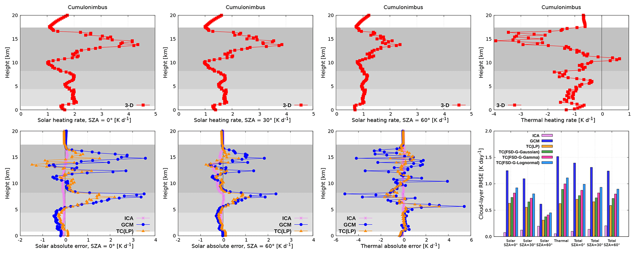
Figure 11Radiative heating rate for the cumulonimbus cloud. The gray-shaded area denotes the cloud layer. The liquid region is shaded light gray, the mixed-phase region is shaded middle gray, and the ice region is shaded dark gray.
We find that 3-D solar radiative transfer has a non-negligible effect at all SZAs (Fig. 11, bottom row). In particular, heating rate differences between ICA and 3-D of about −0.5 K d−1 (up to −30 %) are observed at SZA of 60∘ and extend throughout the majority of the ice region. These differences exceed those reported by Di Giuseppe and Tompkins (2003b), which in turn surpass those previously documented by Barker et al. (1999) and Fu et al. (2000) for solar radiation in deep convective clouds. In the underlying stratiform layer, the ICA error is comparatively small, but it increases again in the bottommost region of shallow cumuli due to their increased side area, where 3-D radiative effects are maximized (Črnivec and Mayer, 2019). A similar picture is identified in the thermal spectral range, where the maximal ICA error of 0.1 K d−1 is observed in the anvil and the cumuliform region, whereas in the stratiform layer the 3-D effect is limited.
In both the solar and thermal spectral ranges, the GCM reveals large errors within the anvil portion and even larger errors in the stratiform layer underneath (Fig. 11, bottom row). The latter are, as expected, a manifestation of considerable horizontal inhomogeneity observed in the stratiform region (recall that its actual FSD is 2 times larger than that of the anvil), which implies that the horizontally homogeneous cloud assumption is violated more in the stratiform region than in the anvil. If the stratiform layer had not been partially shielded by the anvil, the errors therein would be even larger. For overhead Sun, for example, we observe an overestimation of solar heating by up to 3.6 K d−1 in the anvil region and 3.5 K d−1 in the stratiform region. Thermal GCM error of cloud-top cooling up to −4.2 K d−1 and that of cloud-base warming up to 3.9 K d−1 is observed within the anvil. Within the stratiform region, thermal cooling is overestimated, with an error of −5.2 K d−1, and thermal warming is overestimated by 5.4 K d−1 in the GCM configuration. This indicates a significant need for proper TC usage when treating deep convection.
All Tripleclouds baseline experiments yield a significant reduction of solar, thermal and total heating rate error when compared to the GCM. The TC(LP) experiment performs best, reducing the cloud-layer RMSE 2- to 3-fold. As an illustration, thermal RMSE of 1.5 K d−1 is reduced to solely 0.6 K d−1. Although the actual LWC and IWC are better approximated with either lognormal or gamma distribution, the assumption of Gaussianity works best in practice. The reason for this is similar as was the case for the cirrus case study: the actual FSD of the cumulonimbus is mostly larger than the global estimate. As the assumed Gaussianity implies the largest difference between the LWC IWC pair, it partly accounts for the missing inhomogeneity degree introduced by global FSD. It is worth noting that, within the stratiform layer (the liquid phase of which is markedly heterogeneous with FSD similar to that of the cirrus case), TC(FSD) experiments represent a considerable improvement compared to the GCM. This could be partially due to radiatively important effect of ice within the stratiform mixed-phase region: the actual FSD of ice is in close proximity to the global estimate, thus acting to reduce the overall TC error in this region.
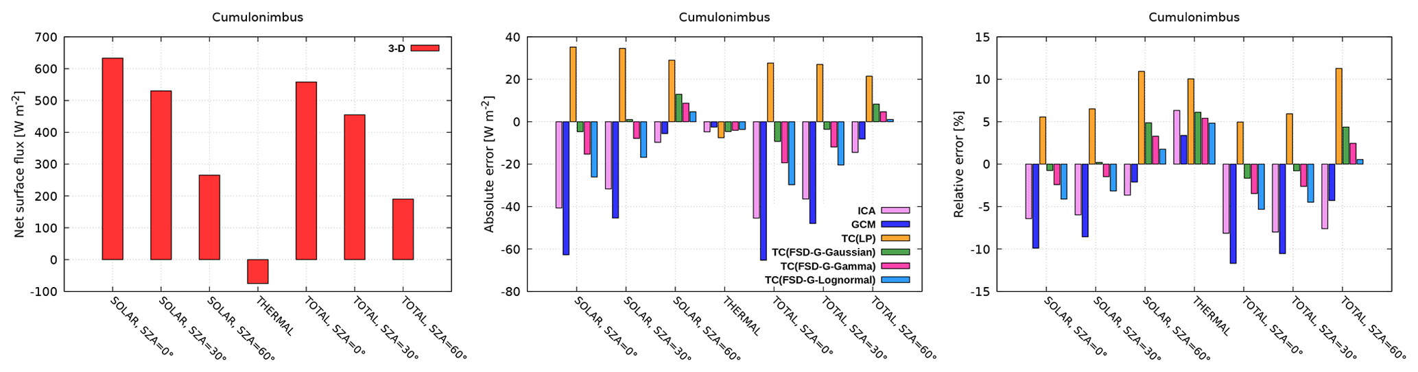
3.3.1 Net surface flux
Figure 12 shows the net surface flux underneath the cumulonimbus. The 3-D radiative effects at the surface are by far largest for the cumulonimbus case, which is a consequence of its large aspect ratio. The daytime net flux in the ICA is underestimated at all SZAs (maximal error of −45 W m−2 or −8 % at overhead Sun), principally due to the cloud-side escape mechanism. The opposing 3-D effect is related to side illumination, where the effective cloud cover (Hinkelman et al., 2007) increases with descending Sun. This casts an elongated shadow, reducing the 3-D net flux, although for the towering cumulonimbus geometry the side escape dominates also at SZA of 60∘. This extensive role of 3-D radiative transfer is consistent with the findings of Di Giuseppe and Tompkins (2005), who showed that the solar error is an asymmetrical function of cloud cover, with the maximum attained at anvil coverage of 30 %–40 %. The majority of previous studies on deep convective systems documented smaller surface ICA error, mostly due to a vast anvil representative of organized convection. For isolated thunderstorms or largely unorganized convection, the greater ICA error as reported herein is presumably more appropriate. According to Rickenbach and Rutledge (1998), such cases constituted about 50 % of all convective events observed during the Tropical Ocean – the Global Atmosphere Coupled Ocean – Atmosphere Response Experiment (TOGA-COARE, Webster and Lukas, 1992). The nighttime surface cooling in the ICA is stronger than in the 3-D radiative transfer (error of −5 W m−2 or 6 %), since realistic cloud-side emission increases downward radiation at the surface (Schäfer et al., 2016).
All deficiencies of the ICA manifest in the GCM as well. Nevertheless, the daytime GCM error is even larger (−65 W m−2 or −12 % at overhead Sun). The horizontally homogeneous GCM cloud emits a greater radiation amount towards the surface compared to the heterogeneous cloudiness in the ICA, leading to a reduced nighttime error.
The baseline Tripleclouds method leads to a significantly improved daytime net flux compared to its representation in the GCM, especially in conjunction with the FSD method. In particular, the GCM error at overhead Sun is reduced by a factor of up to 6. At SZA of 60∘, the daytime GCM error is practically entirely depleted as it is reduced by a factor of 8 when TC is applied with the lognormal assumption. The TC slightly degrades nocturnal surface budget compared to the GCM, although for the lognormal assumption this degradation is marginal (relative error increased by 1 %).
The fact that all TC solar calculations have a positive bias with respect to the ICA can be partly also due to the assumed overlap being too maximal. This leads to an increased amount of direct solar radiation reaching the ground in the TC calculation compared to that in the ICA. It should however be kept in mind that the partial effective treatment of 3-D radiative effects (e.g., cloud-side escape) in the TC scheme simultaneously leads to an increased diffuse surface radiation compared to its counterpart in the ICA. Future studies should try to disentangle and quantify these effects.
In overall summary, the baseline Tripleclouds setup performed well for the apparently most complex deep convective scenario. Nevertheless, improved configurations should be further sought in the future. It would be especially intriguing to contemplate how to better treat the mixed-phase region, where the actual FSD of liquid phase is extremely large. Thus similar optimizations as for the cirrus case study could be introduced, although in the mixed-phase region of the present cumulonimbus, where the actual FSD of ice is close to the global estimate, caution needs to be taken when asymmetrically splitting the cloud fraction.
This study aims to advance the conceptual understanding of radiative transfer in marine stratocumulus, midlatitude cirrus and tropical deep convective clouds. The focus is laid on the issues related to misrepresentation of cloud horizontal inhomogeneity in coarse-resolution weather and climate models, which are tackled with the aid of the Tripleclouds radiative solver. The TC method, primarily introduced by SH08, is an approach accounting for horizontal cloud inhomogeneity by using two regions in each vertical layer to represent the cloud (as opposed to one which is the convention of traditional cloud models). One of these regions is utilized to represent the optically thicker portion of the cloud, whereas the other region represents the residual optically thinner portion. The challenge is to properly set the pair of liquid ice water content defining the two cloudy regions and divide the layer cloudiness geometrically in the corresponding two parts. The primary objective of the present work was to evaluate the global FSD estimate together with different assumptions for cloud condensate distribution, which are commonly applied in models. The TC concept was recently integrated in the efficient δ-Eddington two-stream radiation scheme (Črnivec and Mayer, 2020) and was used herein to answer these questions within the scope of the libRadtran library. For our study, we chose three intrinsically contrasting cloud types which should reflect diverse cloud conditions occurring globally. These high-resolution cloud field data allow us to gain important insights about small-scale cloud variability and give the opportunity to compare the actual modeled variability with the global estimate or other existing parameterizations. For each cloud type, various TC experiments were evaluated against a 3-D benchmark calculation. These results were compared with the GCM computation utilizing homogeneous layer cloudiness which can be viewed as the upper limit for the tolerable TC error. Moreover, the ICA approximation was compared with the 3-D benchmark to quantify the error related to neglected horizontal photon transport. A systematic investigation of cloud-layer heating rate and net surface flux error was provided for each selected cloud case.
It was found that in the majority of applications, the ICA is significantly more accurate than the GCM experiment. This indicates a large potential for Tripleclouds, which reduces the error related to unresolved cloud structure, but not to horizontal photon transport. Regarding the optimal TC configuration, which aims to minimize the radiative error, the exact conclusions depend on each particular cloud type. In general, the simplest TC arrangement using a globally constant FSD and geometrically halving the layer cloudiness worked best for the apparently most complex deep convective scenario. In the case of stratocumulus and cirrus, an improved TC performance was highly desired. To that end, the second objective of the present study was to assess recent advanced FSD parameterizations, characterizing systematic departures from global mean cloud variability observed for liquid and ice phase. For the stratocumulus, an optimization in terms of a parametric FSD relationship portraying reduced horizontal variability at overcast conditions lead to a substantially improved TC realization. For extremely heterogeneous cirrus, on the other hand, allocating the greater portion to the optically thinner part of the cloud (e.g., approximately of layer cloudiness in the solar part of the spectrum) proved to be of crucial importance in the TC settings, eliminating the vast majority of GCM errors. These findings are in support of cloud regime dependent approaches, which ought to be used in radiation schemes of next-generation atmospheric models. Whereas current GCMs do not explicitly predict cloud meteorological regimes (e.g., whether model cloudiness appears in the form of cumulus or stratocumulus), they have the ability to diagnose cloud type based on temperature and humidity fields (Norris, 1998). An alternative is to consider the physical processes responsible for cloud formation as imprinted in the parameterization schemes activated to generate cloudiness within a model grid box (e.g., shallow convection as opposed to large-scale saturation). We thereby propose that the TC configuration should be adequately adjusted according to cloud type.
This work provides the physical understanding of radiative errors, in particular those stemming from neglected cloud horizontal heterogeneity, for three fundamentally contrasting cloud cases. This is a necessary first step for properly setting the TC parameters in its possible future operational usage. A more comprehensive documentation of radiative errors would necessitate the examination of the full parameter space of in-cloud horizontal variability and cloud geometry. As an illustration, Črnivec and Mayer (2019) investigated the 3-D, ICA and NWP-type radiative transfer for an evolving shallow cumulus and showed that the errors depend on the stage of cloud field life cycle. Although Črnivec and Mayer (2019) examined radiative errors at the resolution of regional NWP models, similar problematics is expected at coarser resolution of larger-scale models as well. A natural extension of the present study therefore appears to be the examination of the full ASTEX data set. The transition from solid stratocumulus to trade cumulus or stratocumulus breakup (Albrecht et al., 1995; Bretherton and Wyant, 1997) seems appealing to study with Tripleclouds, since it is often associated with increased horizontal heterogeneity (Wang and Lenschow, 1995; Wood, 2012). Whereas in the current study a single stratocumulus was investigated, the future work should distinguish between clean (marine) and polluted (continental) cases. For the ASTEX field experiment, namely, substantial variations in clean and polluted air masses were reported, which affected both cloud properties and drizzle. Furthermore, in order to properly consider clouds in sheared environments, the vertical overlap rules in the present TC implementation have to be generalized. Finally, if the subgrid horizontal photon transport is to be accounted for in a proficient manner, the two-stream equations need to be extended to include terms representing the in-layer horizontal radiative energy exchange between the cloud and the cloud-free part of the grid box as well as that between the optically thicker and thinner parts of the cloud. We currently investigate some of these topics, which will be addressed in a forthcoming study.
The radiative transfer package (libRadtran 2.0.4) is available at https://doi.org/10.5281/zenodo.4262916 (Črnivec and Mayer, 2020b) under the GNU General Public License v2. The Zenodo repository additionally archives data for the stratocumulus, cirrus and cumulonimbus clouds, as well as the MYSTIC benchmark radiation data, which are accessible under Creative Commons Attribution 4.0 International License (CC BY 4.0). The scripts to process the cloud data and to perform the radiative transfer simulations are available at the same repository under CC BY 4.0 as well.
NC conceived the study, processed the cloud data, performed radiative transfer simulations and evaluated the results. BM upgraded the Tripleclouds implementation within libRadtran to include the ice-phase cloud processing for the purpose of this research. NC prepared the paper draft, whereby BM provided valuable input for its final version.
The authors declare that they have no conflict of interest.
This research contributes to the project “B4 – Radiative heating and cooling at cloud scale and its impact on dynamics” of the Transregional Collaborative Research Center “Waves to Weather”. We acknowledge Marko Korošec Weather Photography (http://www.markokorosec.net, last access: 12 April 2021) for the stunning thunderstorm photo. We thank Fabian Jakub for providing the stratocumulus data, Robin Hogan and Sophia Schäfer for providing the cirrus data, and Tobias Zinner for providing the cumulonimbus data. We thank Lina Boljka for providing insightful literature, as well as Mihail Manev for proofreading the paper and providing helpful comments. Finally, we would like to thank both reviewers, namely Robin Hogan and Hartwig Deneke, for their constructive comments, which substantially improved the quality of our paper.
This research has been supported by the Deutsche Forschungsgemeinschaft (DFG) (grant no. SFB/TRR 165 Waves To Weather).
This paper was edited by Sylwester Arabas and reviewed by Robin Hogan and Hartwig Deneke.
Agee, E. M., Chen, T. S., and Dowell, K. E.: A review of mesoscale cellular convection, B. Am. Meteorol. Soc., 54, 1004–1012, https://doi.org/10.1175/1520-0477(1973)054<1004:AROMCC>2.0.CO;2, 1973. a, b
Albrecht, B. A., Bretherton, C. S., Johnson, D., Scubert, W. H., and Frisch, A. S.: The Atlantic Stratocumulus transition experiment – ASTEX, B. Am. Meteorol. Soc., 76, 889–904, https://doi.org/10.1175/1520-0477(1995)076<0889:TASTE>2.0.CO;2, 1995. a, b
Anderson, G. P., Clough, S. A., Kneizys, F. X., Chetwynd, J. H., and Shettle, E. P.: AFGL Atmospheric Constituent Profiles (0–120 km), Tech. Rep., AFGL (OPI), Hanscom Air Force Base, Massachusetts, USA, AFGL-TR-86-0110, 1986. a
Atkinson, B. W. and Zhang, J. W.: Mesoscale shallow convection in the atmosphere, Rev. Geophys., 34, 403–431, https://doi.org/10.1029/96RG02623, 1996. a
Barker, H. W., Wielicki, B. A., and Parker, L.: A parameterization for computing grid-averaged solar fluxes for inhomogeneous marine boundary layer clouds, Part II: Validation using satellite data, J. Atmos. Sci., 53, 2304–2316, https://doi.org/10.1175/1520-0469(1996)053<2304:APFCGA>2.0.CO;2, 1996. a
Barker, H. W., Stephens, G. L., and Fu, Q.: The sensitivity of domain averaged solar fluxes to assumptions about cloud geometry, Q. J. Roy. Meteor. Soc., 125, 2127–2152, https://doi.org/10.1002/qj.49712555810, 1999. a, b
Bauer, P., Thorpe, A., and Brunet, G.: The quiet revolution of numerical weather prediction, Nature, 525, 47–55, 2015. a
Baur, F., Keil, C., and Craig, G. C.: Soil moisture-precipitation coupling over Central Europe: Interactions between surface anomalies at different scales and the dynamical implication, Q. J. Roy. Meteor. Soc., 144, 2863–2875, 2018. a
Bony, S., Stevens, B., Frierson, D. M. W., Jakob, C., Kageyama, M., Pincus, R., Shepherd, T. G., Sherwood, S. C., Siebesma, A. P., Sobel, A. H., Watanabe, M., and Webb, M. J.: Clouds, circulation and climate sensitivity, Nat. Geosci., 8, 261–268, https://doi.org/10.1038/ngeo2398, 2015. a
Boucher, O., Randall, D., Artaxo, P., Bretherton, C., Feingold, G., Forster, P., Kerminen, V.-M., Kondo, Y., Liao, H., Lohmann, U., Rasch, P., Satheesh, S. K., Sherwood, S., Stevens, B., and Zhang, X. Y.: Clouds and aerosols, in: Climate Change 2013: The Physical Science Basis, Cambridge University Press, Cambridge, UK, https://doi.org/10.1017/CBO9781107415324.016, 2013. a
Boutle, I. A., Abel, S. J., Hill, P. G., and Morcrette, C. J.: Spatial variability of liquid cloud and rain: observations and microphysical effects, Q. J. Roy. Meteor. Soc., 140, 583–594, https://doi.org/10.1002/qj.2140, 2014. a, b, c
Bretherton, C. S. and Khairoutdinov, M. F.: Convective self‐aggregation feedbacks in near‐global cloud‐resolving simulations of an aquaplanet, J. Adv. Model. Earth Sy., 7, 1765–1787, https://doi.org/10.1002/2015MS000499, 2015. a
Bretherton, C. S. and Wyant, M. C.: Moisture transport, lower-tropospheric stability, and decoupling of cloud-topped boundary layers, J. Atmos. Sci., 54, 148–167, https://doi.org/10.1175/1520-0469(1997)054<0148:MTLTSA>2.0.CO;2, 1997. a
Bugliaro, L., Zinner, T., Keil, C., Mayer, B., Hollmann, R., Reuter, M., and Thomas, W.: Validation of cloud property retrievals with simulated satellite radiances: a case study for SEVIRI, Atmos. Chem. Phys., 11, 5603–5624, https://doi.org/10.5194/acp-11-5603-2011, 2011. a
Cahalan, R. F., Ridgway, W., Wiscombe, W. J., Bell, T. L., and Snider, J. B.: The albedo of fractal stratocumulus clouds, J. Atmos. Sci., 51, 2434–2455, https://doi.org/10.1175/1520-0469(1994)051<2434:TAOFSC>2.0.CO;2, 1994. a, b
Cahalan, R. F., Silberstein, D., and Snider, J. B.: Liquid water path and plane-parallel albedo bias during ASTEX, J. Atmos. Sci., 52, 3002–3012, https://doi.org/10.1175/1520-0469(1995)052<3002:LWPAPP>2.0.CO;2, 1995. a
Carlin, B., Fu, Q., Lohmann, U., Mace, G. G., Sassen, K., and Comstock, J. M.: High-cloud horizontal inhomogeneity and solar albedo bias, J. Climate, 15, 2321–2339, https://doi.org/10.1175/1520-0442(2002)015<2321:HCHIAS>2.0.CO;2, 2002. a, b, c, d
Črnivec, N. and Mayer, B.: Quantifying the bias of radiative heating rates in numerical weather prediction models for shallow cumulus clouds, Atmos. Chem. Phys., 19, 8083–8100, https://doi.org/10.5194/acp-19-8083-2019, 2019. a, b, c, d, e, f
Črnivec, N. and Mayer, B.: The incorporation of the Tripleclouds concept into the δ-Eddington two-stream radiation scheme: solver characterization and its application to shallow cumulus clouds, Atmos. Chem. Phys., 20, 10733–10755, https://doi.org/10.5194/acp-20-10733-2020, 2020a. a, b, c, d, e, f, g
Črnivec, N. and Mayer, B.: Code and data for GMD article: “Towards an improved treatment of cloud-radiation interaction in weather and climate models: exploring the potential of the Tripleclouds method for various cloud types using libRadtran 2.0.4”, Zenodo, https://doi.org/10.5281/zenodo.4262916, 2020b. a
Davies, R.: The effect of finite geometry on the three-dimensional transfer of solar irradiance in clouds, J. Atmos. Sci., 35, 1712–1725, 1978. a
Deardorff, J. W.: On the distribution of mean radiative cooling at the top of a stratocumulus-capped mixed layer, Q. J. Roy. Meteor. Soc., 107, 191–202, https://doi.org/10.1002/qj.49710745112, 1981. a
Di Giuseppe, F. and Tompkins, A. M.: Effect of spatial organization on solar radiative transfer in three-dimensional idealized stratocumulus cloud fields, J. Atmos. Sci., 60, 1774–1794, https://doi.org/10.1175/1520-0469(2003)060<1774:EOSOOS>2.0.CO;2, 2003a. a, b, c
Di Giuseppe, F. and Tompkins, A. M.: Three-dimensional radiative transfer in tropical deep convective clouds, J. Geophys. Res.-Atmos., 108, 4741, https://doi.org/10.1029/2003JD003392, 2003b. a, b, c, d
Di Giuseppe, F. and Tompkins, A. M.: Impact of cloud cover on solar radiative biases in deep convective regimes, J. Atmos. Sci., 62, 1989–2000, https://doi.org/10.1175/JAS3442.1, 2005. a, b
Di Giuseppe, F. and Tompkins, A. M.: Generalizing cloud overlap treatment to include the effect of wind shear, J. Atmos. Sci., 72, 2865–2876, https://doi.org/10.1175/JAS-D-14-0277.1, 2015. a
Emde, C., Buras-Schnell, R., Kylling, A., Mayer, B., Gasteiger, J., Hamann, U., Kylling, J., Richter, B., Pause, C., Dowling, T., and Bugliaro, L.: The libRadtran software package for radiative transfer calculations (version 2.0.1), Geosci. Model Dev., 9, 1647–1672, https://doi.org/10.5194/gmd-9-1647-2016, 2016. a
Evans, K. F. and Wiscombe, W. J.: An algorithm for generating stochastic cloud fields from radar profile statistics, Atmos. Res., 72, 263–289, https://doi.org/10.1016/j.atmosres.2004.03.016, 2004. a
Fauchez, T., Cornet, C., Szczap, F., Dubuisson, P., and Rosambert, T.: Impact of cirrus clouds heterogeneities on top-of-atmosphere thermal infrared radiation, Atmos. Chem. Phys., 14, 5599–5615, https://doi.org/10.5194/acp-14-5599-2014, 2014. a
Fu, Q., Cribb, M. C., Barker, H. W., Krueger, S. K., and Grossman, A.: Cloud geometry effects on atmospheric solar absorption, J. Atmos. Sci., 57, 1156–1168, https://doi.org/10.1175/1520-0469(2000)057<1156:CGEOAS>2.0.CO;2, 2000. a, b
Fu, Q., Smith, M., and Yang, Q.: The impact of cloud radiative effects on the tropical tropopause layer temperatures, Atmosphere-Basel, 9, 377, https://doi.org/10.3390/atmos9100377, 2018. a
Geleyn, J. F. and Hollingsworth, A.: An economical analytical method for the computation of the interaction between scattering and line absorption of radiation, Contrib. Atmos. Phys., 52, 1–16, 1979. a
Guichard, F. and Couvreaux, F.: A short review of numerical cloud-resolving models, Tellus A, 69, 1373578, https://doi.org/10.1080/16000870.2017.1373578, 2017. a
Haigh, J. D.: Radiative heating in the lower stratosphere and the distribution of ozone in a two‐dimensional model, Q. J. Roy. Meteor. Soc., 110, 167–185, https://doi.org/10.1002/qj.49711046312, 1984. a
Harrington, J. Y., Feingold, G., and Cotton, W. R.: Radiative impacts on the growth of a population of drops within simulated summertime arctic stratus, J. Atmos. Sci., 57, 766–785, https://doi.org/10.1175/1520-0469(2000)057<0766:RIOTGO>2.0.CO;2, 2000. a
Hartmann, D. L., Gasparini, B., Berry, S. E., and Blossey, P. N.: The life cycle and net radiative effect of tropical anvil clouds, J. Adv. Model. Earth Sy., 10, 3012–3029, https://doi.org/10.1029/2018MS001484, 2018. a
Haynes, J. M. and Stephens, G. L.: Tropical oceanic cloudiness and the incidence of precipitation: Early results from CloudSat, Geophys. Res. Lett., 34, L09811, https://doi.org/10.1029/2007GL029335, 2007. a
Heiblum, R. H., Pinto, L., Altaratz, O., Dagan, G., and Koren, I.: Core and margin in warm convective clouds – Part 1: Core types and evolution during a cloud's lifetime, Atmos. Chem. Phys., 19, 10717–10738, https://doi.org/10.5194/acp-19-10717-2019, 2019. a
Heus, T. and Jonker, H. J. J.: Subsiding shells around shallow cumulus clouds, J. Atmos. Sci., 65, 1003–1018, https://doi.org/10.1175/2007JAS2322.1, 2008. a
Heymsfield, A. J.: Precipitation development in stratiform ice clouds: A microphysical and dynamical study, J. Atmos. Sci., 34, 367–381, https://doi.org/10.1175/1520-0469(1977)034<0367:PDISIC>2.0.CO;2, 1977. a
Hill, P. G., Hogan, R. J., Manners, J., and Petch, J. C.: Parametrizing the horizontal inhomogeneity of ice water content using CloudSat data products, Q. J. Roy. Meteor. Soc., 138, 1784–1793, https://doi.org/10.1002/qj.1893, 2012. a, b, c
Hill, P. G., Morcrette, C. J., and Boutle, I. A.: A regime‐dependent parametrization of subgrid‐scale cloud water content variability, Q. J. Roy. Meteor. Soc., 141, 1975–1986, https://doi.org/10.1002/qj.2506, 2015. a, b, c
Hinkelman, L. M., Evans, K. F., Clothiaux, E. E., Ackerman, T. P., and Stackhouse Jr., P. W.: The effect of cumulus cloud field anisotropy on domain-averaged solar fluxes and atmospheric heating rates, J. Atmos. Sci., 64, 3499–3520, https://doi.org/10.1175/2010JCLI3752.1, 2007. a
Hogan, R. J. and Illingworth, A. J.: Parameterizing ice cloud inhomogeneity and the overlap of inhomogeneities using cloud radar data, J. Atmos. Sci., 60, 756–767, https://doi.org/10.1175/1520-0469(2003)060<0756:PICIAT>2.0.CO;2, 2003. a, b
Hogan, R. J. and Kew, S. F.: A 3D stochastic cloud model for investigating the radiative properties of inhomogeneous cirrus clouds, Q. J. Roy. Meteor. Soc., 131, 2585–2608, https://doi.org/10.1256/qj.04.144, 2005. a, b, c, d, e, f, g
Hogan, R. J., Bouniol, D., Ladd, D. N., O'Connor, E. J., and Illingworth, A. J.: Absolute calibration of 94/95-GHz radars using rain, J. Atmos. Ocean. Tech., 20, 572–580, 2003. a
Hogan, R. J., Schäfer, S. A. K., Klinger, C., and Mayer, B.: Representing 3-D cloud radiation effects in two-stream schemes: 2. Matrix formulation and broadband evaluation, J. Geophys. Res.-Atmos., 121, 8583–8599, https://doi.org/10.1002/2016JD024875, 2016. a
Hogan, R. J., Fielding, M. D., Barker, H. W., Villefranque, N., and Schäfer, S. A.: Entrapment: An important mechanism to explain the shortwave 3D radiative effect of clouds, J. Atmos. Sci., 76, 2123–2141, https://doi.org/10.1175/JAS-D-18-0366.1, 2019. a, b
Hu, Y. X. and Stamnes, K.: An accurate parameterization of the radiative properties of water clouds suitable for use in climate models, J. Climate, 6, 728–742, https://doi.org/10.1175/1520-0442(1993)006<0728:AAPOTR>2.0.CO;2, 1993. a
Jakub, F. and Mayer, B.: A three-dimensional parallel radiative transfer model for atmospheric heating rates for use in cloud resolving models – The TenStream solver, J. Quant. Spectrosc. Ra., 163, 63–71, https://doi.org/10.1016/j.jqsrt.2015.05.003, 2015. a, b
Jakub, F. and Mayer, B.: 3-D radiative transfer in large-eddy simulations – experiences coupling the TenStream solver to the UCLA-LES, Geosci. Model Dev., 9, 1413–1422, https://doi.org/10.5194/gmd-9-1413-2016, 2016. a
Jakub, F. and Mayer, B.: The role of 1-D and 3-D radiative heating in the organization of shallow cumulus convection and the formation of cloud streets, Atmos. Chem. Phys., 17, 13317–13327, https://doi.org/10.5194/acp-17-13317-2017, 2017. a
Johnson, R. H., Rickenbach, T. M., Rutledge, S. A., Ciesielski, P. E., and Schubert, W. H.: Trimodal Characteristics of Tropical Convection, J. Atmos. Sci., 12, 2397–2418, https://doi.org/10.1175/1520-0442(1999)012<2397:TCOTC>2.0.CO;2, 1999. a
Khairoutdinov, M. F. and Randall, D. A.: Cloud resolving modeling of the ARM Summer 1997 IOP: Model formulation, results, uncertainties, and sensitivities, J. Atmos. Sci., 60, 607–625, https://doi.org/10.1175/1520-0469(2003)060<0607:CRMOTA>2.0.CO;2, 2003. a
Klemp, J. B. and Wilhelmson, R. B.: The simulation of three-dimensional convective storm dynamics, J. Atmos. Sci., 35, 1070–1096, https://doi.org/10.1175/1520-0469(1978)035<1070:TSOTDC>2.0.CO;2, 1978. a
Klinger, C. and Mayer, B.: Three-dimensional Monte Carlo calculation of atmospheric thermal heating rates, J. Quant. Spectrosc. Ra., 144, 123–136, https://doi.org/10.1016/j.jqsrt.2014.04.009, 2014. a
Klinger, C. and Mayer, B.: The neighboring column approximation (NCA) – A fast approach for the calculation of 3D thermal heating rates in cloud resolving models, J. Quant. Spectrosc. Ra., 168, 17–28, https://doi.org/10.1016/j.jqsrt.2015.08.020, 2016. a, b
Klinger, C., Mayer, B., Jakub, F., Zinner, T., Park, S.-B., and Gentine, P.: Effects of 3-D thermal radiation on the development of a shallow cumulus cloud field, Atmos. Chem. Phys., 17, 5477–5500, https://doi.org/10.5194/acp-17-5477-2017, 2017. a
Klinger, C., Feingold, G., and Yamaguchi, T.: Cloud droplet growth in shallow cumulus clouds considering 1-D and 3-D thermal radiative effects, Atmos. Chem. Phys., 19, 6295–6313, https://doi.org/10.5194/acp-19-6295-2019, 2019. a
Kobayashi, T.: Parameterization of reflectivity for broken cloud fields, J. Atmos. Sci., 45, 3034–3045, 1988. a
Lang, S., Tao, W.-K., Ciffeli, R., Olson, W., Halverson, J., Rutledge, S., and Simpson, J.: Improving simulations of convective systems from TRMM LBA: Easterly and Westerly Regimes, J. Atmos. Sci., 64, 1141–1164, https://doi.org/10.1175/JAS3879.1, 2007. a, b
Manabe, S.: Climate and ocean circulation: 1. The atmospheric circulation and the hydrology of the earth's surface, Mon. Weather Rev., 97, 739–774, 1969. a
Marshak, A., Davis, A., Wiscombe, W., and Cahalan, R.: Radiative smoothing in fractal clouds, J. Geophys. Res.-Atmos., 100, 26247–26261, https://doi.org/10.1029/95JD02895, 1995. a
Mayer, B.: Radiative transfer in the cloudy atmosphere, EPJ Web Conf., 1, 75–99, https://doi.org/10.1140/epjconf/e2009-00912-1, 2009. a, b
Mitchell, D. L.: A Model Predicting the Evolution of Ice Particle Size Spectra and Radiative Properties of Cirrus Clouds, Part I: Microphysics, J. Atmos. Sci., 51, 797–816, https://doi.org/10.1175/1520-0469(1994)051<0797:AMPTEO>2.0.CO;2, 1994. a
Naud, C. M., Del Genio, A., Mace, G. G., Benson, S., Clothiaux, E. E., and Kollias, P.: Impact of dynamics and atmospheric state on cloud vertical overlap, J. Climate, 21, 1758–1770, https://doi.org/10.1175/2007JCLI1828.1, 2008. a
Norris, J. R.: Low cloud type over the ocean from surface observations, Part I: Relationship to surface meteorology and the vertical distribution of temperature and moisture, J. Atmos. Sci., 11, 369–382, https://doi.org/10.1175/1520-0442(1998)011<0369:LCTOTO>2.0.CO;2, 1998. a
Oreopoulos, L. and Cahalan, R. F.: Cloud inhomogeneity from MODIS, J. Climate, 18, 5110–5124, https://doi.org/10.1175/JCLI3591.1, 2005. a, b
Pincus, R., McFarlane, S. A., and Klein, S. A.: Albedo bias and the horizontal variability of clouds in subtropical marine boundary layers: Observations from ships and satellites, J. Geophys. Res.-Atmos., 104, 6183–6191, https://doi.org/10.1029/1998JD200125, 1999. a, b, c
Pincus, R., Barker, H. W., and Morcrette, J.-J.: A fast, flexible, approximate technique for computing radiative transfer in inhomogeneous cloud fields, J. Geophys. Res.-Atmos., 108, 4376, https://doi.org/10.1029/2002JD003322, 2003. a
Randall, D. A.: Conditional Instability of the First Kind Upside-Down, J. Atmos. Sci., 37, 125–130, https://doi.org/10.1175/1520-0469(1980)037<0125:CIOTFK>2.0.CO;2, 1980. a
Randall, D. A., Khairoutdinov, M., Arakawa, A., and Grabowski, W.: Breaking the cloud parameterization deadlock, B. Am. Meteorol. Soc., 84, 1547–1564, https://doi.org/10.1175/BAMS-84-11-1547, 2003. a
Rickenbach, T. M. and Rutledge, S. A.: Convection in TOGA COARE: Horizontal scale, morphology, and rainfall production, J. Atmos. Sci., 55, 2715–2729, https://doi.org/10.1175/1520-0469(1998)055<2715:citchs>2.0.co;2, 1998. a
Rossow, W. B., Delo, C., and Cairns, B.: Implications of the observed mesoscale variations of clouds for the Earth's radiation budget, J. Climate, 15, 557–585, https://doi.org/10.1175/1520-0442(2002)015<0557:IOTOMV>2.0.CO;2, 2002. a, b
Schäfer, S. A. K.: What is the global impact of 3-D cloud-radiation interactions? Doctoral dissertation, University of Reading, Reading, UK, 138 pp., 2016. a
Schäfer, S. A. K., Hogan, R. J., Klinger, C., Chiu, J. C., and Mayer, B.: Representing 3-D cloud radiation effects in two-stream schemes: 1. Longwave considerations and effective cloud edge length, J. Geophys. Res.-Atmos., 121, 8567–8582, https://doi.org/10.1002/2016JD024876, 2016. a
Schneider, T., Teixeira, J., Bretherton, C. S., Brient, F., Pressel, K. G., Schär, C., and Siebesma, A. P.: Climate goals and computing the future of clouds, Nat. Clim. Change, 7, 3–5, https://doi.org/10.1038/nclimate3190, 2017. a, b
Shonk, J. K. P. and Hogan, R. J.: Tripleclouds: An efficient method for representing horizontal cloud inhomogeneity in 1D radiation schemes by using three regions at each height, J. Climate, 21, 2352–2370, https://doi.org/10.1175/2007JCLI1940.1, 2008. a
Shonk, J. K. P. and Hogan, R. J.: Effect of improving representation of horizontal and vertical cloud structure on the Earth's global radiation budget, Part II: The global effects, Q. J. Roy. Meteor. Soc., 136, 1205–1215, https://doi.org/10.1002/qj.646, 2010. a, b
Shonk, J. K. P., Hogan, R. J., Edwards, J. M., and Mace, G. G.: Effect of improving representation of horizontal and vertical cloud structure on the Earth's global radiation budget, Part I: Review and parameterization, Q. J. Roy. Meteor. Soc., 136, 1191–1204, https://doi.org/10.1002/qj.647, 2010. a, b, c, d, e, f
Simpson, J., Adler, R. F., and North, G. R.: A proposed Tropical Rainfall Measuring Mission (TRMM) satellite, B. Am. Meteorol. Soc., 69, 278–295, https://doi.org/10.1175/1520-0477(1988)069<0278:APTRMM>2.0.CO;2, 1988. a
Simpson, J., Kummerow, C., Tao, W.-K., and Adler, R. F.: On the Tropical Rainfall Measuring Mission, Meteorol. Atmos. Phys., 60, 19–36, 1996. a
Smith, S. A. and Del Genio, A. D.: Analysis of aircraft, radiosonde, and radar observations in cirrus clouds observed during FIRE II: The interactions between environmental structure, turbulence, and cloud microphysical properties, J. Atmos. Sci., 58, 451–461, 2001. a, b
Stephens, G. L., Gabriel, P. M., and Tsay, S.-C.: Statistical radiative transport in one-dimensional media and its application to the terrestrial atmosphere, Transport Theor. Stat., 20, 139–175, https://doi.org/10.1080/00411459108203900, 1991. a
Stephens, G. L., Vane, D. G., Boain, R. J., Mace, G. G., Sassen, K., Wang, Z., Illingworth, A. J., O'Connor, E. J., Rossow, W. B., Durden, S. L., Miller, S. D., Austin, R. T., Benedetti, A., Mitrescu, C., and CloudSat Science Team: The CloudSat mission and the A-Train: A new dimension of space-based observations of clouds and precipitation, B. Am. Meteorol. Soc., 83, 1771–1790, https://doi.org/10.1175/BAMS-83-12-1771, 2002. a
Stephens, G. L., Vane, D. G., Tanelli, S., Im, E., Durden, S. L., Rokey, M., Reinke, D., Partain, P., Mace, G. G., Austin, R., L'Ecuyer, T., Haynes, J. M., Lebsock, M., Suzuki, K., Waliser, D., Wu, D., Kay, J., Gettelmann, A., Wang, Z., and Marchand, R.: CloudSat mission: Performance and early science after the first year of operation, J. Geophys. Res.-Atmos., 113, D00A18, https://doi.org/10.1029/2008JD009982, 2008. a
Stevens, B. and Bony, S.: What are climate models missing?, Science, 340, 1053–1054, 2013. a
Stevens, B., Moeng, C.-H., and Sullivan, P. P.: Large-eddy simulations of radiatively driven convection: Sensitivities to the representation of small scales, J. Atmos. Sci., 56, 3963–3984, https://doi.org/10.1175/1520-0469(1999)056<3963:LESORD>2.0.CO;2, 1999. a
Stevens, B., Moeng, C.-H., Ackerman, A. S., Bretherton, C. S., Chlond, A., de Roode, S., Edwards, J., Golaz, J.-C., Jiang, H., Khairoutdinov, M., Kirkpatrick, M. P., Lewellen, D. C., Lock, A., Müller, F., Stevens, D. E., Whelan, E., and Zhu, P.: Evaluation of large-eddy simulations via observations of nocturnal marine stratocumulus, Mon. Weather Rev., 133, 1443–1462, https://doi.org/10.1175/MWR2930.1, 2005. a, b
Su, H., Jiang, J. H., Vane, D. G., and Stephens, G. L.: Observed vertical structure of tropical oceanic clouds sorted in large‐scale regimes, Geophys. Res. Lett., 35, L24704, https://doi.org/10.1029/2008GL035888, 2008. a
Tao, W.-K. and Simpson, J.: Goddard cumulus ensemble model, Part I: Model description, Terr. Atmos. Ocean. Sci., 4, 35–72, 1993. a, b
Tao, W.-K., Simpson, J., Baker, D., Braun, S., Chou, M.-D., Ferrier, B., Johnson, D., Khain, A., Lang, S., Lynn, B., Shie, C.-L., Starr, D., Sui, C.-H., Wang, Y., and Wetzel, P.: Microphysics, radiation and surface processes in the Goddard Cumulus Ensemble (GCE) model, Meteorol. Atmos. Phys., 82, 97–137, 2003. a
Várnai, T. and Davies, R.: Effects of cloud heterogeneities on shortwave radiation: Comparison of cloud-top variability and internal heterogeneity, J. Atmos. Sci., 56, 4206–4224, https://doi.org/10.1175/1520-0469(1999)056<4206:EOCHOS>2.0.CO;2, 1999. a
Wang, S. and Lenschow, D. H.: An observational study of the role of penetrating cumulus in a marine stratocumulus-topped boundary layer, J. Atmos. Sci., 52, 2902–2922, https://doi.org/10.1175/1520-0469(1995)052<2778:AOSOTR>2.0.CO;2, 1995. a
Webster, P. J. and Lukas, R.: TOGA COARE: The Coupled Ocean-Atmosphere Response Experiment, B. Am. Meteorol. Soc., 73, 1377–1416, https://doi.org/10.1175/1520-0477(1992)073<1377:TCTCOR>2.0.CO;2, 1992. a
Webster, P. J. and Stephens, G. L.: Tropical upper-tropospheric extended clouds: Inferences from winter MONEX, J. Atmos. Sci., 37, 1521–1541, https://doi.org/10.1175/1520-0469(1980)037<1521:TUTECI>2.0.CO;2, 1980. a
Welch, R. M. and Wielicki, B. A.: Reflected fluxes for broken clouds over a Lambertian surface, J. Atmos. Sci., 46, 1384–1395, 1989. a
Wissmeier, U., Buras, R., and Mayer, B.: paNTICA: A fast 3D radiative transfer scheme to calculate surface solar irradiance for NWP and LES models, J. Appl. Meteorol. Clim., 52, 1698–1715, https://doi.org/10.1175/JAMC-D-12-0227.1, 2013. a
Wood, R.: Stratocumulus clouds, Mon. Weather Rev., 140, 2373–2423, https://doi.org/10.1175/MWR-D-11-00121.1, 2012. a, b
Wood, R. and Hartmann, D. L.: Spatial variability of liquid water path in marine boundary layer clouds: The importance of mesoscale cellular convection, J. Climate, 19, 1748–1764, 2006. a
Yang, P., Liou, K. N., Wyser, K., and Mitchell, D.: Parameterization of the scattering and absorption properties of individual ice crystals, J. Geophys. Res.-Atmos., 105, 4699–4718, https://doi.org/10.1029/1999JD900755, 2000. a
Zhong, W., Hogan, R. J., and Haigh, J. D.: Three-dimensional radiative transfer in midlatitude cirrus clouds, Q. J. Roy. Meteor. Soc., 134, 199–215, https://doi.org/10.1002/qj.182, 2008. a, b, c, d, e, f, g
Zinner, T., Marshak, A., Lang, S., Martins, J. V., and Mayer, B.: Remote sensing of cloud sides of deep convection: towards a three-dimensional retrieval of cloud particle size profiles, Atmos. Chem. Phys., 8, 4741–4757, https://doi.org/10.5194/acp-8-4741-2008, 2008. a
Zuidema, P. and Evans, K. P.: On the validity of independent pixel approximation for boundary layer clouds observed during ASTEX, J. Geophys. Res.-Atmos., 103, 6059–6074, https://doi.org/10.1029/98JD00080, 1998. a, b
It should be noted, however, that the studies of Hogan and Kew (2005) and Zhong et al. (2008) use coarser horizontal grid spacing (1.56 km). We adopted the cirrus data from Schäfer (2016), where the simulation of Hogan and Kew (2005) had been rerun with higher resolution (horizontal grid spacing of 50 m), whereby we eventually smeared the data onto the grid with a horizontal grid spacing of 100 m to facilitate the Monte Carlo radiative transfer simulations.
The fact that the deep convective cloud is practically not sheared makes it a perfect target to study the performance of our current Tripleclouds implementation, which is not yet capable of representing an arbitrary vertical overlap.