A discontinuous Galerkin finite-element model for fast channelized lava flows v1.0

Lava flows present a significant natural hazard to communities around volcanoes and are typically slow-moving (<1 to 5 cm s⁻¹) and laminar. Recent lava flows during the 2018 eruption of Kīlauea volcano, Hawai'i, however, reached speeds as high as 11 m s⁻¹ and were transitional to turbulent. The Kīlauea flows formed a complex network of braided channels departing from the classic rectangular channel geometry often employed by lava flow models. To investigate these extreme dynamics we develop a new lava flow model that incorporates nonlinear advection and a nonlinear expression for the fluid viscosity. The model makes use of novel discontinuous Galerkin (DG) finite-element methods and resolves complex channel geometry through the use of unstructured triangular meshes. We verify the model against an analytic test case and demonstrate convergence rates of $\mathcal{P}+\mathrm{1}/\mathrm{2}$ for polynomials of degree 𝒫. Direct observations recorded by unoccupied aerial systems (UASs) during the Kīlauea eruption provide inlet conditions, constrain input parameters, and serve as a benchmark for model evaluation.

1 Introduction

On 3 May 2018, Kīlauea volcano on the island of Hawai'i began to erupt from new fissures in the lower East Rift Zone at the center of the Leilani Estates subdivision. Before ceasing in early August 2018, the lava flows destroyed over 650 structures and caused significant damage to infrastructure and essential facilities. During the second half of the eruption, the flow field established a complex braided channel system (which is common to many basaltic flows), originating from fissure number 8 (see Fig. 1). The “Fissure 8” flows were unique in the fact that they produced channelized flows reaching speeds as high as 15 m s⁻¹ (Patrick et al., 2019). These high speeds, coupled with channel geometry (e.g., constrictions) produced Reynolds numbers (Re>3000) that were significantly higher than typical lava flows. To investigate these extreme dynamics we develop a new channelized lava flow computer model named a discontinuous Galerkin finite-element model for fast channelized lava flows version 1.0.

This paper is organized as follows. In Sect. 1.1–1.3, we present the motivation for this work, as well as background on the mathematical tools we employ. In Sect. 2, we present the mathematical model and the bottom stress calculation and detail its nuances. We present the discontinuous Galerkin (DG) numerical discretization of the mathematical model in Sect. 3 and verify the model in Sect. 4. In Sect. 5, we evaluate the model against observations of lava flows from the 2018 eruption of Kīlauea volcano. We present misfit errors and root-mean-square errors (RMSEs) for the velocity field from a braided channel section of Fissure 8 and provide quantitative insight into physical quantities of the lava flow field in this area, including its thickness and viscosity. We close the paper in Sect. 6 with some discussion and conclusions.

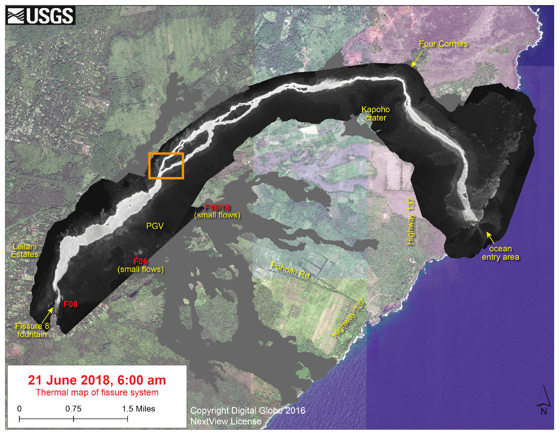
Figure 1 A satellite image (colored, in the background, by DigitalGlobe) overlaid with a thermal aerial orthomosaic (grayscale) where the white and light gray areas reveal the path of the Fissure 8 flow channel as it was on 21 June 2018. Data and map by USGS. The orange rectangle depicts the area of UAS site 8 from where the video we analyzed was captured on 22 June 2018. The flat gray areas south of the active flow channel demarcate the areas inundated by lava during the early stages of the eruption. The top of the image is north. PGV is the Puna Geothermal Ventures power plant that was heavily impacted by the lava.

1.1 Motivation

Typical “operational” lava flow models simulate unconfined lava flow in a 2D plan view (e.g., SCIARA, Crisci et al., 2004; MAGFLOW, Vicari et al., 2007; LavaPL, Connor et al., 2012; VOLCFLOW, Kelfoun and Vargas, 2015) using either cellular automata or depth-averaged equations in an effort to forecast the area of land inundated by the lava. It is often difficult, however, for these models to accurately reproduce the complicated braided channel network such as those created by Fissure 8. These braided channel networks are common in natural flows (e.g., Dietterich and Cashman, 2014), and understanding the evolution of the velocity, rheology, and temperature fields (e.g. in response to pulsating effusion) within these channels is critical to hazard mitigation (Patrick et al., 2019). Direct measurements of lava properties in situ is usually extremely difficult and dangerous. Modeling lava dynamics within the bounds of an established channel can help to better understand material properties of the flowing lava and inform models and decisions.

Previous attempts to model channelized lava flows have made use of simple heuristic formulas such as Jeffreys equation for laminar flows (Harris and Rowland, 2015) or Chezy approximations for higher-speed flows (Baloga et al., 1995). While convenient, the use of these equations has largely been dictated by the fact that it has been difficult to obtain the physical data necessary for advanced modeling efforts (e.g., channel domain boundaries, inlet boundary conditions, topography). However, with the advent of unoccupied aerial systems (UASs, or “drones”) and their ability to survey active lava fields, we now have access to the data required by sophisticated numerical methods.

1.2 Shallow-water equations for fast lava flows

Commensurate with this development in observational capabilities, we introduce a numerical method for modeling fast-moving lava flows in complex channels. The high Reynolds number associated with these lava flows, coupled with the fact that the total length of the flows (on the order of kilometers) is much greater than the flow depth (on the order of meters), means that the dynamics can be well approximated by two-dimensional depth-integrated equations for mass, momentum, and energy. In particular, we utilize a system of dynamical equations known as the “shallow water equations” (Saint-Venant, 1851), which quantify average horizontal velocities and the depth of flow. These equations are traditionally used to model free surface flows in coastal oceanic regions, estuaries, and rivers (Dawson and Mirabito, 2008), although they have been used to model debris flows (George and Iverson, 2014) and lava flows (Costa and Macedonio, 2005) as well. The main assumption in the shallow water theory is that the fluid pressure is hydrostatic; gravitational acceleration dominates vertical accelerations in the fluid, and the pressure is calculated via the vertical momentum equation. The formulation of the shallow water equations that we utilize is designed specifically for advection-dominated flows (Kubatko et al., 2006), and the pressure gradient term is formulated so that the dynamical equations are well balanced; steady states are preserved, and no artificial motion is induced by numerical artifacts (see Conroy, 2014, for a full derivation of the dynamical equations from conservation principles).

Lava flows are distinct from hydrological free surface flows in the sense that lava transfers heat to its surroundings; as lava effuses from a vent it cools along lateral flow boundaries and can form solid walls (“levees”) that prevent the lava from spreading to nearby regions. If lava effusion extends for several days, long channels may form that efficiently transport lava from the vent to the flow front. The speed at which the lava flows through the channel system depends on the viscosity of the lava, which in turn is highly dependent on the temperature and chemical composition of the lava (e.g., Griffiths, 2000). The presence of crystals and/or bubbles in the lava can make its viscosity non-Newtonian (Manga et al., 1998; Mader et al., 2013) and thus strongly dependent on stress gradients and the thermal properties of the lava. To reflect this strong dependence on temperature, we solve a depth-integrated energy equation that quantifies the thermal evolution of the lava as it interacts with its environment. The depth-integrated energy equation is coupled to the shallow water equations through a thermally dependent nonlinear stress term that reflects the rheology of the lava and can account for the presence of crystals and/or bubbles in the lava flow.

The logistical key to using shallow water equations to model lava flow dynamics rests on the development of the non-Newtonian bottom stress term. Typical friction drag laws do not take into account the viscosity of the fluid (due to the assumption that the fluids inertial acceleration is much greater than its internal resistance). However, in our particular case the flow is not fully turbulent; internal resistance needs to be taken into account in some fashion. Thus, we express the stress at the bottom boundary as a function of the temperature and the vertical stress gradient (which is a function on the vorticity). We solve a thermal boundary layer problem to calculate the temperature at the bottom boundary and utilize the vorticity to determine a virtual length scale over which the interior velocity goes from the depth-averaged value to zero. This results in a bottom stress approximation that is void of a friction factor (e.g., Manning's n) and allows scientists to study physical properties of the lava that are difficult to measure directly (e.g., viscosity). For example, application of the model to the Kīlauea 2018 Fissure 8 lava flows reveals that the lava behaved as a shear thickening fluid due to the high bubble content (≈ 50 %) with a large capillary number, which agrees well with the recent lab experiments of Lev et al. (2020).

1.3 The discontinuous Galerkin finite-element method

Because closed-form analytic solutions do not exist to the nonlinear shallow water equations and energy equation, we construct approximate solutions to these equations using discontinuous Galerkin (DG) finite-element methods (Cockburn and Shu, 2001), which have been used to successfully model other geophysical fluid flows including coastal ocean circulation (Kärnä et al., 2018), hurricanes (Dawson et al., 2011), avalanches (Patra et al., 2006), and debris flows (Conroy and George, 2021). The DG finite-element method differs from continuous Galerkin (CG) finite-element methods in that the DG method solves an integral (or weak) form of the mathematical equations over individual elements and utilizes a solution space that is discontinuous across element boundaries. This allows the DG method to resolve steep gradients that form in the numerical solution, such as the thermodynamic gradients that form at lava channel wall boundaries. Even though the DG method is discontinuous it still conserves mass both locally and globally by utilizing a numerical flux function (introduced by finite-volume methods; see LeVeque (2002) for instance) that takes the discontinuous state of physical properties at element boundaries and creates a consistent flow of information from element to element (Cockburn and Shu, 2001).

Further, the DG method has been shown to be highly parallelizable using high-performance computing (e.g., Kubatko et al., 2009, and Patra et al., 2006) and it is amenable to unstructured numerical meshes. The latter feature is important when resolving geometrically complex boundaries of a given fluid domain, such as the flow fields commonly produced by basaltic flows. For instance, the lava flows that effused from Fissure 8 formed a complicated network of braided channels, with multiple locations of branching and merging. In addition, obstructions such as large lava rafts or preexisting structures caused local disruptions in the flow field, making it difficult to evaluate the dynamics using a simplified one-dimensional channelized model, such as those that use a classical rectangular channel geometry (Harris and Rowland, 2015). To account for these complexities, our new lava flow model discretizes the lava channel domain with an unstructured triangular mesh. This reduces model error as it pertains to a representation of the lava flow domain and is important when reproducing localized flow features of the lava field, such as the jet visible in Fig. 4.

Model verification consists of solving an analytic test case using forcing functions that we choose to exactly satisfy the equations of motion, and results indicate that for smooth solutions the method converges to the exact solution at a rate of $\mathcal{P}+\mathrm{1}/\mathrm{2}$ for polynomials of degree 𝒫.

2 Mathematical model

Fluid flow on sloped terrain can be quantified in a Cartesian coordinate (x, y, z) system over a time-dependent domain Ω(t)∈ℝ³ by solving Eulerian conservation equations of mass, linear momentum, and energy,

$$\begin{array}{}\text{(1)}& {\displaystyle }& {\displaystyle \frac{\partial \mathit{\rho }}{\partial t}}+\mathrm{\nabla }\cdot \left(\mathit{\rho }\mathit{u}\right)=\mathrm{0},\text{(2)}& {\displaystyle }& {\displaystyle \frac{\partial }{\partial t}}\left(\mathit{\rho }\mathit{u}\right)+\mathit{\rho }\mathit{u}\cdot \mathrm{\nabla }\mathit{u}+\mathrm{\nabla }p-{\left({\mathrm{\nabla }}^{\prime }\mathit{\tau }\right)}^{\prime }={\mathit{f}}_{\text{b}},\text{(3)}& {\displaystyle }& {\displaystyle }\mathit{\rho }{c}_p{\displaystyle \frac{\partial T}{\partial t}}+\mathit{\rho }{c}_p\left(\mathit{u}\cdot \mathrm{\nabla }T\right)-\mathrm{\nabla }\cdot \mathit{q}=\dot{q}.\end{array}$$

In Eqs. (1)–(3), ρ is the fluid density, $\mathit{u}=(u,v,w{)}^{\prime }$ is the fluid velocity vector, $\mathrm{\nabla }={\left(\frac{\partial }{\partial x},\frac{\partial }{\partial y},\frac{\partial }{\partial z}\right)}^{\prime }$ is the gradient operator, p is the pressure, and τ is the stress term,

$$\begin{array}{}\text{(4)}& \mathit{\tau }=\left[\begin{array}{ccc}{\mathit{\tau }}_{xx}& {\mathit{\tau }}_{xy}& {\mathit{\tau }}_{xz}\\ {\mathit{\tau }}_{yx}& {\mathit{\tau }}_{yy}& {\mathit{\tau }}_{yz}\\ {\mathit{\tau }}_{zx}& {\mathit{\tau }}_{zy}& {\mathit{\tau }}_{zz}\end{array}\right].\end{array}$$

We denote the x component of gravitational acceleration that is tangential to the sloped surface by g_x; g_y is the y component of gravitational acceleration that is tangential to the sloped surface, and g_z is gravitational acceleration that is normal to the sloped surface. Collectively, these terms form the body force vector f_b= (g_x, g_y, g_z)^′ acting on the fluid. T is the temperature of the fluid, c_p is the specific heat capacity of the fluid, $\mathit{q}={\left(k_T\frac{\partial T}{\partial x},k_T\frac{\partial T}{\partial y},k_T\frac{\partial T}{\partial z}\right)}^{\prime }$ is the heat flux through the fluid (k_T is a conduction heat transfer coefficient that measures the spread of heat within the fluid), and $\dot{q}$ quantifies the generation and dissipation of heat within the fluid.

Equations (1) and (2), taken together, are the Navier–Stokes equations and quantify the force dynamics acting on the fluid (see Conroy, 2014, for a derivation from first principles). Equation (3) is the thermal energy equation: it quantifies the transport of energy through the fluid due to internal temperature gradients and differences between the fluid temperature and the temperature of the surrounding medium (see Moran et al., 2003, for instance). To apply Eqs. (1)–(4) to channelized lava flow we need to supplement them with appropriate boundary conditions and define the stress matrix τ. Here, we assume that the system of equations given by Eqs. (1)–(3) are subject to the following kinematic, dynamic, and thermal boundary conditions:

• Channel wall boundary condition:
  no normal flow $\mathit{u}\cdot \widehat{\mathit{n}}=\mathrm{0}$;
  no pressure gradient, $\partial p/\partial \widehat{\mathit{n}}=\mathrm{0}$;
  slip velocity, $\mathit{u}\cdot \widehat{\mathit{t}}=f({\mathit{\tau }}_{\text{wall}},{\mathit{\sigma }}_{\text{wall}})$;
  heat loss via conduction, $\mathit{q}\cdot \widehat{\mathit{n}}=\left(k_T/h_{\text{w}}\right)\left(T-T_{\text{wall}}\right)$.

• Inlet boundary condition:
  prescribed velocity, $\mathit{u}\cdot \widehat{\mathit{n}}=\text{prescribed}$;
  prescribed pressure, p=prescribed;
  prescribed heat content, ρc_pT=prescribed.

• Outlet boundary condition:
  zero change in normal velocity, $\partial \mathit{u}/\partial \widehat{\mathit{n}}=\mathrm{0}$;
  zero change in pressure, $\partial p/\partial \widehat{\mathit{n}}=\mathrm{0}$;
  zero change in heat content, $\mathit{\rho }{c}_p\partial T/\partial \widehat{\mathit{n}}=\mathrm{0}$.

• Free surface boundary condition at z=ζ:
  no relative normal flow,
  $\partial \mathit{\zeta }/\partial t=-u(\partial \mathit{\zeta }/\partial x)-v\partial (\mathit{\zeta }/\partial y)+w$;
  atmospheric pressure, p=p_atm;
  surface shear stress, ${\mathit{\tau }}_{{\text{s}}_x}=-{\mathit{\tau }}_{xx}(\partial \mathit{\zeta }/\partial x)-{\mathit{\tau }}_{yx}(\partial \mathit{\zeta }/\partial y)+{\mathit{\tau }}_{zx}$, ${\mathit{\tau }}_{{\text{s}}_y}=-{\mathit{\tau }}_{xy}(\partial \mathit{\zeta }/\partial x)-{\mathit{\tau }}_{yy}(\partial \mathit{\zeta }/\partial y)+{\mathit{\tau }}_{zy}$;
  heat loss via radiation and convection,
  $\mathit{q}\cdot \widehat{\mathit{n}}=\mathit{ϵ}{\mathit{\sigma }}_B\left(T^{\mathrm{4}}-T_{\text{atm}}^{\mathrm{4}}\right)+k_{\text{c}}{\left(T-T_{\text{atm}}\right)}^{\frac{\mathrm{4}}{\mathrm{3}}}$.

• Bottom boundary condition at $z=-h$:
  no slip velocity, u=0;
  bottom shear stress, ${\mathit{\tau }}_{{\text{b}}_x}={\mathit{\tau }}_{xx}(\partial h/\partial x)+{\mathit{\tau }}_{yx}(\partial h/\partial y)+{\mathit{\tau }}_{zx}$, ${\mathit{\tau }}_{{\text{b}}_y}={\mathit{\tau }}_{xy}(\partial h/\partial x)+{\mathit{\tau }}_{yy}(\partial h/\partial y)+{\mathit{\tau }}_{zy}$;
  heat loss via conduction, $\mathit{q}\cdot \widehat{\mathit{n}}=(k_{\text{b}}/h_{\text{b}})\left(T-T_{\text{ground}}\right)$.

In the boundary conditions above, $\widehat{\mathit{n}}$ is the unit normal vector to the wall boundary, outlet boundary, inlet boundary, moving free surface, and bottom boundary, respectively; $\widehat{\mathit{t}}$ is the unit tangential vector to the wall; τ_wall is the tangential shear stress at the wall; and σ_wall is the normal stress at the wall. We denote the temperature at the wall by T_w, k_w is the thermal conductivity of the wall, and h_w is the thickness of the thermal boundary layer through which heat is conducted from the lava flow to the wall. We measure the free surface, ζ, relative to a steady depth of flow, h(x,y), that serves as the zero datum in the z direction (see Fig. 2). The surface forces acting on the free surface consist of the atmospheric pressure, p_atm, along with a surface shear stress applied by the wind ${\mathit{\tau }}_{\text{s}}=({\mathit{\tau }}_{{\text{s}}_x},{\mathit{\tau }}_{{\text{s}}_y}{)}^{\prime }$. Heat transfer from the lava surface to the surrounding atmosphere is dominantly due to radiation and air convection, where ϵ is the emissivity of the lava, σ_B is the Stefan–Boltzmann constant, T_atm is the temperature of the surrounding atmosphere, and k_c is the convection heat transfer coefficient. The main resisting force in dense shallow mass high-speed flows comes from the bottom stress, ${\mathit{\tau }}_{\text{b}}=({\mathit{\tau }}_{{\text{b}}_x},{\mathit{\tau }}_{{\text{b}}_y}{)}^{\prime }$, which is a function of the temperature of the lava at the basal boundary, where T_ground is the temperature of the ground and h_b is the depth of the thermal boundary layer through which heat is transferred from the lava to the ground.

Figure 2 A vertical cross section along the center line of the flow, showing the coordinates (x and z, with y the across-flow direction) and the heat transfer mechanisms considered in the model (conduction to the base, advection by the flow, and heat loss by radiation and convection at the surface).

Theoretically, we could define τ and solve Eqs. (1)–(3) along with the prescribed boundary conditions to model channelized lava flows. In practice, however, we need to simplify Eqs. (1)–(3) to make the solution more tractable. More specifically, we assume the following: (i) the lava flow field is incompressible, (ii) vertical accelerations in the lava are dominated by gravity, (iii) lava flow lengths are much greater than the flow depth, and (iv) horizontal flow speeds are large enough that stress gradients are dominated by the first two columns of the stress matrix τ.

Assumption (i) reduces the conservation of mass equation to $\mathrm{\nabla }\cdot \mathit{u}=\mathrm{0}$, while assumptions (ii) and (iv) reduce the z-momentum equation to

$${\displaystyle \frac{\partial p}{\partial z}}=\mathit{\rho }{g}_z,$$

which we can leverage to determine the pressure. Integrating from the free surface ζ down to a given z coordinate yields

$$\begin{array}{}\text{(5)}& p=p_{\text{atm}}+\mathit{\rho }{g}_z\left(\mathit{\zeta }-z\right).\end{array}$$

We assume that gradients in p_atm are negligible and the horizontal pressure gradient in Eq. (2) becomes

$$\stackrel{\mathrm{‾}}{\mathrm{\nabla }}p=\stackrel{\mathrm{‾}}{\mathrm{\nabla }}\left(\mathit{\rho }{g}_z\mathit{\zeta }\right),$$

where $\stackrel{\mathrm{‾}}{\mathrm{\nabla }}={\left(\frac{\partial }{\partial x},\frac{\partial }{\partial y}\right)}^{\prime }$. We further simplify the mathematical model and eliminate the vertical dimension by integrating $\mathrm{\nabla }\cdot \mathit{u}=\mathrm{0}$ and Eqs. (2) and (3) over the depth of the lava flow (from −h to ζ). We then apply Leibniz's integral rule, utilize the free-surface and bottom boundary conditions, assume the density is constant, and simplify the resulting expression to arrive at the following depth-integrated equations:

$$\begin{array}{}\text{(6)}& {\displaystyle \frac{\partial H}{\partial t}}+{\displaystyle \frac{\partial }{\partial x}}\left(H\stackrel{\mathrm{‾}}{u}\right)+{\displaystyle \frac{\partial }{\partial y}}\left(H\stackrel{\mathrm{‾}}{v}\right)=\mathrm{0},\text{(7)}& {\displaystyle }\begin{array}{rl}& {\displaystyle \frac{\partial H\stackrel{\mathrm{‾}}{u}}{\partial t}}+{\displaystyle \frac{\partial }{\partial x}}\left(H{\stackrel{\mathrm{‾}}{u}}^{\mathrm{2}}\right)+{\displaystyle \frac{\partial }{\partial y}}\left(H\stackrel{\mathrm{‾}}{u}\stackrel{\mathrm{‾}}{v}\right)+H{\displaystyle \frac{\partial }{\partial x}}\left(g_z\mathit{\zeta }\right)+H{g}_x=\\ & {\displaystyle \frac{\mathrm{1}}{\mathit{\rho }}}\left({\mathit{\tau }}_{{\text{s}}_x}-{\mathit{\tau }}_{{\text{b}}_x}+f_x\right),\end{array}\text{(8)}& {\displaystyle }\begin{array}{rl}& {\displaystyle \frac{\partial H\stackrel{\mathrm{‾}}{v}}{\partial t}}+{\displaystyle \frac{\partial }{\partial x}}\left(H\stackrel{\mathrm{‾}}{u}\stackrel{\mathrm{‾}}{v}\right)+{\displaystyle \frac{\partial }{\partial y}}\left(H{\stackrel{\mathrm{‾}}{v}}^{\mathrm{2}}\right)+H{\displaystyle \frac{\partial }{\partial y}}\left(g_z\mathit{\zeta }\right)+H{g}_y=\\ & {\displaystyle \frac{\mathrm{1}}{\mathit{\rho }}}\left({\mathit{\tau }}_{{\text{s}}_y}-{\mathit{\tau }}_{{\text{b}}_x}+f_y\right),\end{array}\text{(9)}& {\displaystyle \frac{\partial H\stackrel{\mathrm{‾}}{T}}{\partial t}}+{\displaystyle \frac{\partial }{\partial x}}\left(H\stackrel{\mathrm{‾}}{u}\stackrel{\mathrm{‾}}{T}\right)+{\displaystyle \frac{\partial }{\partial y}}\left(H\stackrel{\mathrm{‾}}{v}\stackrel{\mathrm{‾}}{T}\right)=q_{\text{s}}+q_{\text{b}}+\stackrel{\mathrm{‾}}{\mathrm{\nabla }}\cdot {\stackrel{\mathrm{‾}}{q}}_i+\dot{\stackrel{\mathrm{‾}}{q}},\end{array}$$

where f_x and f_y are the x component and y component of the depth-averaged gradient of the shear stresses acting on vertical fluid planes, q_s is the heat flux through the free surface, q_b is the heat flux at the bottom boundary, $\stackrel{\mathrm{‾}}{\mathrm{\nabla }}\cdot {\stackrel{\mathrm{‾}}{q}}_i$ quantifies depth-averaged internal conduction, and $\dot{\stackrel{\mathrm{‾}}{q}}$ represents depth-averaged internal heat generation and dissipation. The depth-averaged velocity, $\stackrel{\mathrm{‾}}{\mathit{u}}=(\stackrel{\mathrm{‾}}{u},\stackrel{\mathrm{‾}}{v})$, and depth-averaged temperature, $\stackrel{\mathrm{‾}}{T}$, are defined as

$$\begin{array}{}\text{(10)}& {\displaystyle }\stackrel{\mathrm{‾}}{u}={\displaystyle \frac{\mathrm{1}}{H}}\underset{-h}{\overset{\mathit{\zeta }}{\int }}u\text{d}z,\text{(11)}& {\displaystyle }\stackrel{\mathrm{‾}}{v}={\displaystyle \frac{\mathrm{1}}{H}}\underset{-h}{\overset{\mathit{\zeta }}{\int }}v\text{d}z,\text{(12)}& {\displaystyle }\stackrel{\mathrm{‾}}{T}={\displaystyle \frac{\mathrm{1}}{H}}\underset{-h}{\overset{\mathit{\zeta }}{\int }}T\text{d}z.\end{array}$$

The above system of depth-integrated equations (Eqs. 6–9) can be further simplified due to the dynamics of high-speed flows. More specifically, f_x and f_y are negligible in high-speed flows except at no-slip and small-slip velocity boundary conditions where large stress gradients form due to the decay of the velocity field to a value of zero (or near zero). In our quantitative analysis of UAS footage from the 2018 Kīlauea eruption, lava flow velocities at channel wall boundaries were much greater than zero, and therefore we utilize a slip (no-flow) channel wall boundary condition and neglect f_x and f_y in this initial version of the model (see Rao and Rajagopai, 1999, for an in depth investigation on channel wall boundary conditions in terms of the slip versus no-slip condition). The surface stress terms $({\mathit{\tau }}_x,{\mathit{\tau }}_y{)}^{\prime }$ in the depth-integrated equations account for wind stress on the lava flow, which we assume to be negligible due to the ratio of the density of air to the density of lava being much less than one. We include the effect of heat conduction at the channel wall boundaries, but we neglect heat conduction in the interior of the lava due to the high speed of the flow, and we set $\stackrel{\mathrm{‾}}{\mathrm{\nabla }}\cdot {\stackrel{\mathrm{‾}}{q}}_i=\mathrm{0}$. Internal heat generation and dissipation can be significant in lava flows with a high crystal content (Griffiths, 2000) and in lava flows in closed tubes (Costa and Macedonio, 2005). The Fissure 8 lava flows were hot with limited crust cover, and samples indicate that the crystal content was low in the channel section that we apply the model to (Gansecki et al., 2019), and therefore we neglect $\dot{\stackrel{\mathrm{‾}}{q}}$ in the current model but plan to include it in future releases.

It can be noted that the pressure gradient terms, $(\mathrm{1}/\mathit{\rho })\stackrel{\mathrm{‾}}{\mathrm{\nabla }}p={\left(H\frac{\partial }{\partial x}\left(g_z\mathit{\zeta }\right),H\frac{\partial }{\partial x}\left(g_z\mathit{\zeta }\right)\right)}^{\prime }$, in Eqs. (7) and (8) are non-conservative product terms that can lead to entropy-violating numerical fluxes if care is not taken in evaluating them numerically (see LeVeque, 2002, for instance). To circumvent this issue, we make use of the fact $H(x,y,t)=\mathit{\zeta }(x,y,t)+h(x,y)$ and rewrite Eqs. (7) and (8) in the conservative form (Kubatko et al., 2006),

$$\begin{array}{}\text{(13)}& {\displaystyle \frac{\partial \mathit{\zeta }}{\partial t}}+{\displaystyle \frac{\partial }{\partial x}}\left(H\stackrel{\mathrm{‾}}{u}\right)+{\displaystyle \frac{\partial }{\partial y}}\left(H\stackrel{\mathrm{‾}}{v}\right)=\mathrm{0},\text{(14)}& {\displaystyle }\begin{array}{rl}& {\displaystyle \frac{\partial H\stackrel{\mathrm{‾}}{u}}{\partial t}}+{\displaystyle \frac{\partial }{\partial x}}\left(H{\stackrel{\mathrm{‾}}{u}}^{\mathrm{2}}+P\right)+{\displaystyle \frac{\partial }{\partial y}}\left(H\stackrel{\mathrm{‾}}{u}\stackrel{\mathrm{‾}}{v}\right)+H{g}_x\\ & =g\mathit{\zeta }{\displaystyle \frac{\partial h}{\partial x}}-{\displaystyle \frac{{\mathit{\tau }}_{{\text{b}}_x}}{\mathit{\rho }}},\end{array}\text{(15)}& {\displaystyle }\begin{array}{rl}& {\displaystyle \frac{\partial H\stackrel{\mathrm{‾}}{v}}{\partial t}}+{\displaystyle \frac{\partial }{\partial x}}\left(H\stackrel{\mathrm{‾}}{u}\stackrel{\mathrm{‾}}{v}\right)+{\displaystyle \frac{\partial }{\partial y}}\left(H{\stackrel{\mathrm{‾}}{v}}^{\mathrm{2}}+P\right)+H{g}_y\\ & =g\mathit{\zeta }{\displaystyle \frac{\partial h}{\partial y}}-{\displaystyle \frac{{\mathit{\tau }}_{{\text{b}}_y}}{\mathit{\rho }}},\end{array}\text{(16)}& {\displaystyle \frac{\partial H\stackrel{\mathrm{‾}}{T}}{\partial t}}+{\displaystyle \frac{\partial }{\partial x}}\left(H\stackrel{\mathrm{‾}}{u}\stackrel{\mathrm{‾}}{T}\right)+{\displaystyle \frac{\partial }{\partial y}}\left(H\stackrel{\mathrm{‾}}{v}\stackrel{\mathrm{‾}}{T}\right)=q_{\text{s}}+q_{\text{b}},\end{array}$$

where $P=\frac{\mathrm{1}}{\mathrm{2}}{g}_z\left(H^{\mathrm{2}}-h^{\mathrm{2}}\right)$ is the pressure flux and $\partial h/\partial x$ and $\partial h/\partial y$ quantify the gradient in the steady reference depth of flow that ζ is measured relative to. We supplement the system of equations given by Eqs. (13)–(16) with initial conditions along with the channel wall, inlet, and outlet boundary conditions. It can be noted that the depth-integrated mass and momentum equations given by Eqs. (13)–(15) are well studied in the literature and are commonly used to model shallow mass flows such as coastal ocean circulation and hurricane storm surge; see, for example, Dawson et al. (2011) and Kubatko et al. (2006). The addition of the energy equation complicates the solution of Eqs. (14) and (15) due to the fact that the bottom stress term, ${\mathit{\tau }}_{\text{b}}=({\mathit{\tau }}_{{\text{b}}_x},{\mathit{\tau }}_{{\text{b}}_y}{)}^{\prime }$, is now a function of both nonlinear velocity gradients and temperature.

2.1 Quantifying the bottom stress term

In the equations of motion (Eqs. 14 and 15), we define the bottom stress term using a Herschel–Bulkley model (Herschel and Bulkley, 1926),

$$\begin{array}{}\text{(17)}& {\mathit{\tau }}_{\text{b}}={\mathit{\tau }}_{zx}=\mathit{\mu }{\displaystyle \frac{\partial \mathit{u}}{\partial z}}+{\mathit{\tau }}_{\text{yield}}\left[\text{sgn}\left({\displaystyle \frac{\partial \mathit{u}}{\partial z}}\right)\right],\end{array}$$

where ${\mathit{\tau }}_{\text{b}}={\mathit{\tau }}_{zx}=({\mathit{\tau }}_{zx},{\mathit{\tau }}_{zy}{)}^{\prime }$, τ_yield is the yield strength of the fluid, sgn denotes the sign of the argument, and μ is the nonlinear viscosity, defined as

$$\begin{array}{}\text{(18)}& \mathit{\mu }=\mathcal{K}{\left|{\displaystyle \frac{\partial \mathit{u}}{\partial z}}\right|}^{n-\mathrm{1}}.\end{array}$$

The symbol 𝒦 in Eq. (18) represents the consistency of the lava and can be modeled solely as a function of temperature, while the power law exponent, n, is typically a function of the particle content (crystals and/or bubbles) of the lava (which in turn can be a function of temperature); see Castruccio et al. (2010) and Castruccio et al. (2014) for example. We quantify the temperature dependency of the lava consistency (𝒦) in a fashion similar to Sonder et al. (2006) and use the Vogel–Fulcher–Tammann (VFT) silicate melt model of Giordano et al. (2008),

$$\begin{array}{}\text{(19)}& \log \left({\displaystyle \frac{\mathcal{K}}{{\mathcal{K}}_{\mathrm{0}}}}\right)=A+{\displaystyle \frac{B}{T\left(\text{K}\right)-C}},\end{array}$$

where A is the value of $\log \mathcal{K}/{\mathcal{K}}_{\mathrm{0}}$ at infinite temperature, 𝒦₀ is a constant set to 1 sⁿ⁻¹, and B and C are parameters that depend on the composition of the lava. The model assumes that A is a constant for all silicate melts regardless of composition, and thus it represents the high temperature limit for silicate melt viscosity. Once the parameter A is fixed then the parameters B and C are determined via a linear ensemble of combinations of oxide components and a subordinate number of multiplicative oxide cross terms; see Giordano et al. (2008) for the full details of the model.

The power law exponent of the viscosity term quantifies the effect that stress gradients have on the material properties of the fluid. A value of n=1 corresponds to a Newtonian fluid, while n<1 or n>1 corresponds to a non-Newtonian fluid. If n>1 then the fluid viscosity increases with increasing shear rate (shear thickening), while if n<1 the fluid viscosity decreases with increasing shear rate (known as shear thinning). Typically, if the lava is sufficiently hot and degassed, then the lava stress can be modeled with a Newtonian approximation and n=1. However, if bubbles and/or crystals are present in the lava (depending on the lava source and the amount of degassing that has occurred), then these structures will deform and realign under an applied shear stress. This consequently causes the viscosity of the lava to become thinner in some situations and thicker in others depending on how the structures rearrange. Lava flows with a high crystal content are typically pseudo-plastic and shear thinning; the crystal structure of the lava resists the flow of the lava and the lava will not flow unless a yield strength is surpassed. In this case, the lava will continue to flow more readily as the shear stress increases. The opposite tends to occur when a lava flow has a high bubble content at higher capillary numbers; large stress gradients in the flow cause the bubbles to rearrange in a fashion that increases the viscosity and the lava behaves as a shear thickening fluid.

The bottom stress term is a function of the velocity gradient evaluated at the bottom boundary, which we do not have access to in the depth-averaged equations, and therefore we define the bottom stress in terms of the depth-averaged velocity as

$$\begin{array}{}\text{(20)}& \begin{array}{rl}& {\mathit{\tau }}_{{\text{b}}_x}\equiv \stackrel{\mathrm{‾}}{\mathit{\mu }}{\displaystyle \frac{\stackrel{\mathrm{‾}}{\mathit{u}}}{{\mathit{\delta }}_z}}+{\mathit{\tau }}_{\text{yield}}\left[\text{sgn}\left({\displaystyle \frac{\stackrel{\mathrm{‾}}{\mathit{u}}}{{\mathit{\delta }}_z}}\right)\right]\\ & \approx \mathit{\mu }{\displaystyle \frac{\partial \mathit{u}}{\partial z}}+{\mathit{\tau }}_{\text{yield}}\left[\text{sgn}\left({\displaystyle \frac{\partial \mathit{u}}{\partial z}}\right)\right],\end{array}\end{array}$$

where

$$\begin{array}{}\text{(21)}& \stackrel{\mathrm{‾}}{\mathit{\mu }}=\mathcal{K}{\left|{\displaystyle \frac{\stackrel{\mathrm{‾}}{\mathit{u}}}{{\mathit{\delta }}_z}}\right|}^{n-\mathrm{1}}.\end{array}$$

It can be noted that in the expression above, ${\mathit{\delta }}_z=({\mathit{\delta }}_{z_x},{\mathit{\delta }}_{z_y}{)}^{\prime }$, is a measure of a virtual length over which the shear stress is applied. We determine δ_z by taking into account the vorticity of the lava flow field, which is defined as

$$\begin{array}{}\text{(22)}& \mathit{\omega }=\left({\displaystyle \frac{\partial w}{\partial y}}-{\displaystyle \frac{\partial v}{\partial z}}\right)\widehat{i}+\left({\displaystyle \frac{\partial w}{\partial x}}-{\displaystyle \frac{\partial u}{\partial z}}\right)\widehat{j}+\left({\displaystyle \frac{\partial u}{\partial y}}-{\displaystyle \frac{\partial v}{\partial x}}\right)\widehat{k},\end{array}$$

where $\widehat{i}$, $\widehat{j}$, and $\widehat{k}$ are unit vectors in the x, y, and z directions, respectively. We solve an auxiliary problem over a pseudo-depth of the lava that consists of an upper mixed layer where $\mathit{u}(x,y,z)\equiv \stackrel{\mathrm{‾}}{\mathit{u}}(x,y)$ and a lower layer where $(\partial u/\partial z,\partial v/\partial z{)}^{\prime }\gg (\partial w/\partial x,\partial w/\partial y{)}^{\prime }$. We assume that the vorticity in the upper layer is equal to the vorticity in the bottom layer (in terms of magnitude) at the coordinate point where $\partial \mathit{u}/\partial z\ne \mathrm{0}$ (i.e., at the interface between the two layers). This allows us to calculate the vorticity in the upper layer and then use this value to determine δ_z. In other words, we answer the following question: given a measure of the vorticity associated with the depth-averaged velocity field, what is the associated length scale over which the depth-averaged velocity must decay to a value of zero (the bottom boundary condition) to ensure that the internal vorticity of the flow is conserved? It can be noted that an implicit assumption in depth-integrated models is that internal friction in the vertical is null compared to the friction at flow boundaries. This, along with assumption (i) and a constant density, implies conservation of vorticity about the $\widehat{i}$ and $\widehat{j}$ directions except at flow boundaries). The key to this approach relies on calculating a measure for the vertical velocity in the upper layer, which we achieve by making use of the kinematic boundary condition,

$$\begin{array}{}\text{(23)}& {\left.{\displaystyle \frac{\partial \mathit{\zeta }}{\partial t}}+u{\displaystyle \frac{\partial \mathit{\zeta }}{\partial x}}\right|}_{z=\mathit{\zeta }}{\left.+v{\displaystyle \frac{\partial \mathit{\zeta }}{\partial y}}\right|}_{z=\mathit{\zeta }}{\left.=w\right|}_{z=\mathit{\zeta }},\end{array}$$

coupled with the depth-integrated continuity Eq. (13) to obtain a measure of the vertical velocity w. More specifically, expanding derivatives in Eq. (13), solving for $\partial \mathit{\zeta }/\partial t$, while substituting this result into Eq. (23) and noting that in the upper layer $(\stackrel{\mathrm{‾}}{u},\stackrel{\mathrm{‾}}{v},\stackrel{\mathrm{‾}}{w})\equiv \left(u\right(\mathit{\zeta }),v(\mathit{\zeta }),w(\mathit{\zeta }\left)\right)$ yields

$$\begin{array}{}\text{(24)}& \stackrel{\mathrm{‾}}{w}=\mathit{\zeta }{\displaystyle \frac{\partial \stackrel{\mathrm{‾}}{u}}{\partial x}}+\mathit{\zeta }{\displaystyle \frac{\partial \stackrel{\mathrm{‾}}{v}}{\partial y}}.\end{array}$$

The relevant vorticity terms in Eq. (22) include the $\widehat{i}$ and $\widehat{j}$ components. By definition, $\partial \stackrel{\mathrm{‾}}{u}/\partial z=\partial \stackrel{\mathrm{‾}}{v}/\partial z=\mathrm{0}$ over the upper layer so that the vorticity component about the x axis is $\partial \stackrel{\mathrm{‾}}{w}/\partial y$ and the vorticity component about the y axis is $\partial \stackrel{\mathrm{‾}}{w}/\partial x$. Because the bottom boundary condition is modeled as a rigid wall where u=0 and the fluid is incompressible, a vorticity layer forms in the fluid near the solid boundary that resists the local rotation of the fluid (this is the reason why the rigid boundary does not deform). The vorticity created at the boundary resists the rotation of the interior and is equal to $\partial v/\partial z$ about the x axis and $\partial u/\partial z$ about the y axis (see Schlichting et al., 1968). Now, if we assume that each vorticity component over the bulk of the flow is equal to each vorticity component in the boundary layer at the coordinate point where $(\partial u/\partial z,\partial v/\partial z{)}^{\prime }$ is no longer equal to zero, then the virtual length over which the shear stress is applied is given by

$$\begin{array}{}\text{(25)}& {\mathit{\delta }}_{z_x}={\displaystyle \frac{\stackrel{\mathrm{‾}}{u}}{\partial \stackrel{\mathrm{‾}}{w}/\partial x}}\text{and}{\mathit{\delta }}_{z_y}={\displaystyle \frac{\stackrel{\mathrm{‾}}{v}}{\partial \stackrel{\mathrm{‾}}{w}/\partial y}}.\end{array}$$

It can be noted that as $(\partial \stackrel{\mathrm{‾}}{w}/\partial x,\partial \stackrel{\mathrm{‾}}{w}/\partial y)$ goes to 0, the vertical stress in the fluid goes to 0. We can rewrite expression (Eq. 25) solely in terms of the depth-averaged variables using Eq. (24):

$$\begin{array}{}\text{(26)}& \begin{array}{rl}& {\mathit{\delta }}_{z_x}=\stackrel{\mathrm{‾}}{u}{\left[{\displaystyle \frac{\partial }{\partial x}}\left(\mathit{\zeta }{\displaystyle \frac{\partial \stackrel{\mathrm{‾}}{u}}{\partial x}}+\mathit{\zeta }{\displaystyle \frac{\partial \stackrel{\mathrm{‾}}{v}}{\partial y}}\right)\right]}^{-\mathrm{1}}\text{and}\\ & {\mathit{\delta }}_{z_y}=\stackrel{\mathrm{‾}}{v}{\left[{\displaystyle \frac{\partial }{\partial y}}\left(\mathit{\zeta }{\displaystyle \frac{\partial \stackrel{\mathrm{‾}}{u}}{\partial x}}+\mathit{\zeta }{\displaystyle \frac{\partial \stackrel{\mathrm{‾}}{v}}{\partial y}}\right)\right]}^{-\mathrm{1}}.\end{array}\end{array}$$

It can be noted that even though we do not explicitly include horizontal shear stresses in the Kīlauea simulations presented in Sect. 5 (due to the high Re number), the virtual length used to quantify the bottom stress as defined in Eq. (26) is a function of horizontal shear within the fluid. Further, we wish to emphasize that the virtual length, δ_z, is non-physical and is not necessarily less than the lava flow thickness (H); it merely is a measure to ensure that $(\stackrel{\mathrm{‾}}{\mathit{u}}-\mathit{0})/{\mathit{\delta }}_z\approx \partial \mathit{u}/\partial z$ at the bottom boundary in a fashion that conserves internal vorticity, i.e., it ensures that the interior of the flow field is irrotational about the $\widehat{i}$ and $\widehat{j}$ coordinate axis.

2.2 Heat transfer

As soon as lava effuses from an active vent it begins to degas and transfer heat to its surroundings. Lava cools through the mechanisms of radiation, conduction, and convection in the air above it (we neglect heating from viscous dissipation, which is small compared to heat loss through radiation and conduction for the low-viscosity flows we are considering here, e.g., Harris and Rowland, 2001). We quantify heat loss due to radiation via Stefan's law (Griffiths, 2000),

$$\begin{array}{}\text{(27)}& q_{\text{s}}={\displaystyle \frac{\mathit{ϵ}{\mathit{\sigma }}_B}{\mathit{\rho }{c}_p}}\left({\stackrel{\mathrm{‾}}{T}}^{\mathrm{4}}-T_{\text{atm}}^{\mathrm{4}}\right),\end{array}$$

where ϵ is the emissivity of the lava, σ_B is the Stefan–Boltzmann constant, and T_atm is the temperature of the surrounding atmosphere in degrees Kelvin. When lava temperatures fall below the solidus (e.g., ∼ 950 C for Kīlauea lavas), buoyancy-driven convection in the air above the lava becomes the dominant mode of heat transfer at the lava surface instead of radiation (due to crust formation) (Griffiths, 2000). In this case we set q_s in the energy equation to

$$\begin{array}{}\text{(28)}& q_{\text{s}}=k_{\text{c}}{\left(\stackrel{\mathrm{‾}}{T}-T_{\text{atm}}\right)}^{\mathrm{4}/\mathrm{3}},\end{array}$$

where k_c is a heat transfer coefficient (e.g., Patrick et al., 2004). We quantify heat transfer from the lava to the ground via conduction (Patrick et al., 2004),

$$\begin{array}{}\text{(29)}& q_{\text{b}}=k_{\text{b}}\left(\stackrel{\mathrm{‾}}{T}-T_{\text{ground}}\right),\end{array}$$

where T_ground=f(x) is the temperature of the ground in contact with the lava flow field and k_b measures the thermal conductivity of the ground. We utilize Eq. (29) to determine the temperature near the bottom boundary of lava flow field which we use to evaluate the nonlinear viscosity in the bottom stress term in the equations of motion. More specifically, we can rewrite Eq. (29) in terms of a depth-dependent thermal boundary layer temperature, T(z),

$$\begin{array}{}\text{(30)}& {\displaystyle \frac{\partial T}{\partial z}}={\displaystyle \frac{{\stackrel{\mathrm{̃}}{k}}_{\text{b}}}{h_{\text{b}}}}\left(T-T_{\text{ground}}\right),\end{array}$$

where ${\stackrel{\mathrm{̃}}{k}}_{\text{b}}$ is the thermal boundary layer conductivity constant and h_b(x,y) is the thickness of the thermal boundary layer (see Fig. 2). We solve Eq. (30) over the thermal boundary layer defined in the z direction from $z=z_{\text{b}}(x,y)$ to $z=-h(x,y)$ by setting z_b(x,y) to a relative zero. We then integrate Eq. (30) over a thermal boundary coordinate defined from $\stackrel{\mathrm{̃}}{z}=\mathrm{0}$ to $\stackrel{\mathrm{̃}}{z}=-h_{\text{b}}(x,y)$. It can be noted that the relationship between $\stackrel{\mathrm{̃}}{z}$ and z is given by $\stackrel{\mathrm{̃}}{z}=z-z_{\text{b}}$ so that $h_{\text{b}}=h-z_{\text{b}}$. Equation (30) is a non-homogeneous, constant coefficient ordinary differential equation that has the following solution:

$$\begin{array}{}\text{(31)}& T\left(\stackrel{\mathrm{̃}}{z}\right)=\left(T_{\text{int}}-T_{\text{ground}}\right)\exp \left({\displaystyle \frac{{\stackrel{\mathrm{̃}}{k}}_{\text{b}}}{h_{\text{b}}}}\stackrel{\mathrm{̃}}{z}\right)+T_{\text{ground}},\end{array}$$

which gives an expression for the temperature profile over the thermal boundary layer of the lava ($\stackrel{\mathrm{̃}}{z}\in [\mathrm{0},-h_{\text{b}}]$). Evaluating Eq. (31) at $\stackrel{\mathrm{̃}}{z}=-h_{\text{b}}$ and setting the interior temperature (T_int) to the depth-integrated value ($\stackrel{\mathrm{‾}}{T}$), we have

$$\begin{array}{}\text{(32)}& T{|}_{\stackrel{\mathrm{̃}}{z}=-h_{\text{b}}}=\left(\stackrel{\mathrm{‾}}{T}-T_{\text{ground}}\right)\exp \left(-{\stackrel{\mathrm{̃}}{k}}_{\text{b}}\right)+T_{\text{ground}}.\end{array}$$

We use this temperature to evaluate the consistency in the bottom stress approximation,

$$\begin{array}{}\text{(33)}& \mathcal{K}{|}_{z=-h}=\mathcal{K}\left(T{|}_{\stackrel{\mathrm{̃}}{z}=-h_{\text{b}}}\right).\end{array}$$

The greater the thermal conductivity of the boundary layer, the closer the boundary temperature is to the ground temperature; however, in general, there is usually a steep gradient in the temperature at the interface between the boundary of the flowing lava and the ground that the lava is conducting heat to. It can be noted that we also use an analogous approach to calculate the temperature of the lava at channel wall boundaries.

2.3 Steady reference depth of flow h

We have two options to calculate the steady reference depth of flow (h) of the lava that we use as a zero datum to measure the free surface from. Our particular choice depends on the inflow data available to the model. For instance, if a full set of temporally varying inflow data is available, we set h equal to the time average thickness associated with the data, i.e.,

$$\begin{array}{}\text{(34)}& h={\displaystyle \frac{\mathrm{1}}{\left(t_{\text{f}}-t_{\text{i}}\right)}}\underset{t_{\text{i}}}{\overset{t_{\text{f}}}{\int }}{\displaystyle \frac{{\mathbf{Q}}_{\text{in}}\cdot \widehat{\mathit{n}}}{{\text{w}}_{\text{in}}}}\left({\mathit{u}}_{\text{in}}\cdot \widehat{\mathit{n}}\right)\text{d}t,\end{array}$$

where ${\mathbf{Q}}_{\text{in}}\cdot \widehat{\mathit{n}}$ is the inflow flux normal to the boundary and w_in is the width of the inflow boundary normal to the flow. If, however, the only inflow data available to the model is a set of time-averaged data, then we set h to the solution of the steady, linear system of equations associated with the full nonlinear system of equations given by Eqs. (13)–(16).

3 Numerical discretization

To develop our numerical methods, we rewrite the system of Eqs. (1) in the compact form,

$$\begin{array}{}\text{(35)}& {\displaystyle \frac{\partial U^{\left(i\right)}}{\partial t}}+\mathrm{\nabla }\cdot {\mathbf{F}}^{\left(i\right)}\left(\mathit{U}\right)=S^{\left(i\right)}\left(\mathit{U}\right),i=\mathrm{1},\mathrm{2},\mathrm{3},\mathrm{4},\end{array}$$

where U⁽ⁱ⁾, F⁽ⁱ⁾, and S⁽ⁱ⁾ are the i-th row entries of the vectors U, S, and the flux function matrix F, defined as

$$\begin{array}{rl}& \mathit{U}=\left[\begin{array}{r}H\\ H\stackrel{\mathrm{‾}}{u}\\ H\stackrel{\mathrm{‾}}{v}\\ H\stackrel{\mathrm{‾}}{T}\end{array}\right],\\ & \mathbf{F}=\left[\begin{array}{cc}H\stackrel{\mathrm{‾}}{u},& H\stackrel{\mathrm{‾}}{v}\\ H{\stackrel{\mathrm{‾}}{u}}^{\mathrm{2}}+P,& H\stackrel{\mathrm{‾}}{u}\stackrel{\mathrm{‾}}{v}\\ H\stackrel{\mathrm{‾}}{u}\stackrel{\mathrm{‾}}{v},& H{\stackrel{\mathrm{‾}}{v}}^{\mathrm{2}}+P\\ H\stackrel{\mathrm{‾}}{u}\stackrel{\mathrm{‾}}{T},& H\stackrel{\mathrm{‾}}{v}\stackrel{\mathrm{‾}}{T}\end{array}\right],\\ & \mathit{S}=\left[\begin{array}{c}\mathrm{0}\\ -g_{x}H+g\mathit{\zeta }\frac{\partial h}{\partial x}-\frac{{\mathit{\tau }}_{{\text{b}}_x}}{\mathit{\rho }}\\ -g_{y}H+g\mathit{\zeta }\frac{\partial h}{\partial y}-\frac{{\mathit{\tau }}_{{\text{b}}_y}}{\mathit{\rho }}\\ q_{\text{s}}+q_{\text{b}}\end{array}\right],\end{array}$$

where $P=\frac{\mathrm{1}}{\mathrm{2}}{g}_z\left(H^{\mathrm{2}}-h^{\mathrm{2}}\right)$.

3.1 Finite-element partition

To apply a DG spatial discretization to our mathematical model (Eq. 35) over a lava flow channel (see Fig. 5, for example), we begin by introducing a partition of the two-dimensional domain Ω. The complexities of the domain boundary, ∂Ω, are such that an unstructured finite-element partition (or mesh) is necessary to properly capture its intricacies. More specifically, we obtain unstructured triangulations (that we denote by 𝒯_h) of the channel domain Ω via an automatic mesh generator known as ADMESH⁺ (Conroy et al., 2012). ADMESH⁺ solves a number of differential equations to calculate a mesh size function that determines local element sizes based on the curvature of the boundary, channel width, and changes in the topography and domain slope to create a high-quality unstructured simplex mesh (the elements are close to equilateral triangles). The only input required by the program is a list of points defining the boundary and the topography of the domain.

3.2 A weak form and the semi-discrete equations

Given the finite-element partition, 𝒯_h, of the domain Ω, we obtain a weak form of Eq. (35) if we first multiply Eq. (35) by a sufficiently smooth test function $\mathit{\psi }(x,y)\in \mathcal{V}$, integrate over each element Ω_j∈𝒯_h, and then integrate the flux term by parts,

$$\begin{array}{}\text{(36)}& \begin{array}{rl}& \underset{{\mathrm{\Omega }}_j}{\int }{\displaystyle \frac{\partial U^{\left(i\right)}}{\partial t}}\mathit{\psi }\text{d}A-\underset{{\mathrm{\Omega }}_j}{\int }{\mathbf{F}}^{\left(i\right)}\cdot \mathrm{\nabla }\mathit{\psi }\text{d}A+\underset{\partial {\mathrm{\Omega }}_j}{\int }\left({\mathbf{F}}^{\left(i\right)}\cdot \widehat{\mathit{n}}\right)\mathit{\psi }\text{d}S=\\ & \underset{{\mathrm{\Omega }}_j}{\int }{S}^{\left(i\right)}\mathit{\psi }\text{d}A,U^{\left(i\right)},\mathit{\psi }\in \mathcal{V},\end{array}\end{array}$$

for $i=\mathrm{1},\mathrm{2},\mathrm{3},\mathrm{4}$ and $j=\mathrm{1},\mathrm{\dots },\mathcal{N}$, where 𝒩 is the total number of elements of the triangulation 𝒯_h. In the equation above, $\widehat{\mathit{n}}$ is the outward unit normal to the element boundary ∂Ω_j. Rather than seek solutions to Eq. (36), we search for solutions in the finite dimensional subspace of functions defined as

$$\begin{array}{}\text{(37)}& {\mathcal{V}}_{hp}=\left\{\mathit{\psi }:\mathit{\psi }\left|{}_{{\mathrm{\Omega }}_j}\right.\in {\mathcal{P}}_{\mathrm{\ell }}\left({\mathrm{\Omega }}_j\right),\forall {\mathrm{\Omega }}_j\right\},\end{array}$$

where 𝒫_ℓ demarcates the space of polynomials of at most degree ℓ that is not necessarily continuous across element boundaries. In other words, given a set of basis functions $\mathit{\varphi }={\left({\mathit{\varphi }}_{\mathrm{0}},{\mathit{\varphi }}_{\mathrm{1}},\mathrm{\dots },{\mathit{\varphi }}_{\mathrm{\ell }}\right)}^{\prime }$, we express the trial solution ($U_h^{\left(i\right)}\in {\mathcal{V}}_{hp}$) and test function (ψ_h∈𝒱_hp) as

$$\begin{array}{}\text{(38)}& U_h^{\left(i\right)}{|}_{{\mathrm{\Omega }}_j}=\sum _{l=\mathrm{0}}^{\mathrm{\ell }}{U}_l^{\left(i\right)}\left(t\right){\mathit{\varphi }}_l\left(\mathbf{x}\right),\end{array}$$

and

$$\begin{array}{}\text{(39)}& {\mathit{\psi }}_h{|}_{{\mathrm{\Omega }}_j}=\sum _{l=\mathrm{0}}^{\mathrm{\ell }}{\mathit{\psi }}_l\left(t\right){\mathit{\varphi }}_l\left(\mathbf{x}\right),\end{array}$$

where ${\left(U_{\mathrm{0}}^{\left(i\right)},U_{\mathrm{1}}^{\left(i\right)},\mathrm{\dots },U_{\mathrm{\ell }}^{\left(i\right)}\right)}^{\prime }$ are the time-dependent degrees of freedom of the finite-element solution and $i=\mathrm{1},\mathrm{2},\mathrm{3},\mathrm{4}$. We use products of Jacobi polynomials of degree ℓ, ${\left\{{\mathcal{P}}_l\right\}}_{l=\mathrm{0}}^{\mathrm{\ell }}$, as the basis for 𝒱_hp. The orthogonal triangular basis is defined in terms of a “collapsed coordinate” system that results in a matrix-free implementation of the method; see Kubatko et al. (2006) for more details. Substituting $U_h^{\left(i\right)}$ and ψ_h into Eq. (36), we arrive at the discrete weak form of the problem: find $U_h^{\left(i\right)}\in {\mathcal{V}}_{hp}$ such that for all test functions ψ_h∈𝒱_hp for $i=\mathrm{1},\mathrm{2},\mathrm{3},\mathrm{4}$, the expression,

$$\begin{array}{}\text{(40)}& \begin{array}{rl}& \underset{{\mathrm{\Omega }}_j}{\int }{\displaystyle \frac{\partial U_h^{\left(i\right)}}{\partial t}}{\mathit{\psi }}_h\text{d}A-\underset{{\mathrm{\Omega }}_j}{\int }{\mathbf{F}}^{\left(i\right)}\left({\mathit{U}}_h\right)\cdot \mathrm{\nabla }{\mathit{\psi }}_h\text{d}A+\underset{\partial {\mathrm{\Omega }}_j}{\int }\left({\widehat{\mathbf{F}}}^{\left(i\right)}\cdot \widehat{\mathit{n}}\right){\mathit{\psi }}_h\text{d}S\\ & =\underset{{\mathrm{\Omega }}_j}{\int }{S}^{\left(i\right)}\left({\mathit{U}}_h\right){\mathit{\psi }}_h\text{d}A,\end{array}\end{array}$$

holds over each element Ω_j∈𝒯_h, where S⁽ⁱ⁾(U_h) is the source term evaluated in 𝒱_hp and ${\widehat{\mathbf{F}}}^{\left(i\right)}$ is a suitably chosen numerical flux.

3.2.1 Numerical flux

The space of functions defined by Eq. (37) is not necessarily continuous across element boundaries, and thus can be dual-valued (see Fig. 3, for example). To remedy this inconsistency, we replace the dual-valued flux in Eq. (36) with a so-called numerical flux ($\widehat{\mathbf{F}}$) that makes use of the left and right limits of the trial solution to produce a single-valued flux across a given element's boundary.

Figure 3 Jump in numerical solution U_h at an element edge ∂Ω_j.

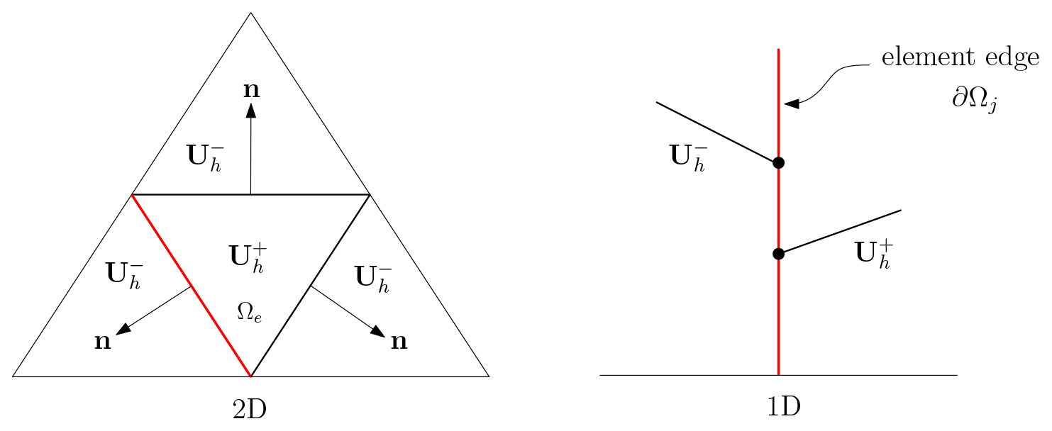
More specifically, given an arbitrary function w_h∈𝒱_hp at an element boundary point x_i, we set the left and right limits of the function to $w_h^{-}\equiv w_h\left({\mathbf{x}}_i^{-}\right)$ and $w_h^{+}\equiv w_h\left({\mathbf{x}}_i^{+}\right)$, respectively. In this work we utilize the local Lax–Friedrichs (LLF) flux, which defines the numerical flux operator as

$$\begin{array}{}\text{(41)}& \begin{array}{rl}& {\widehat{\mathbf{F}}}^{\left(i\right)}\cdot \widehat{\mathit{n}}\\ & ={\displaystyle \frac{\mathrm{1}}{\mathrm{2}}}\left({\mathbf{F}}^{(i,+)}+{\mathbf{F}}^{(i,-)}\right)\cdot \widehat{\mathit{n}}-{\displaystyle \frac{\mathrm{1}}{\mathrm{2}}}\left|{\mathit{\lambda }}_{\text{max}}\right|\left(U_h^{(i,+)}-U_h^{(i,-)}\right),\\ & \text{for}i=\mathrm{1},\mathrm{2},\mathrm{3},\mathrm{4},\end{array}\end{array}$$

where λ_max is the maximum eigenvalue of the normal (to the element edges) Jacobian matrix. When solutions to Eq. (35) are sufficiently smooth, we can rewrite Eq. (35) in the quasi-linear form,

$$\begin{array}{}\text{(42)}& {\displaystyle \frac{\partial \mathit{U}}{\partial t}}+{\mathbf{J}}_x{\left(\mathit{U}\right)}_x+{\mathbf{J}}_{\text{y}}{\left(\mathit{U}\right)}_y=\mathit{S},\end{array}$$

where the Jacobian matrices $\left({\mathbf{J}}_{ij}=\frac{\partial F_i}{\partial x_j}\right)$ are

$${\mathbf{J}}_x=\left[\begin{array}{cccccc}\mathrm{0}& \mathrm{1}& & \mathrm{0}& & \mathrm{0}\\ & & & & & \\ g_{z}H-{\stackrel{\mathrm{‾}}{u}}^{\mathrm{2}}& \mathrm{2}\stackrel{\mathrm{‾}}{u}& & \mathrm{0}& & \mathrm{0}\\ & & & & & \\ -\stackrel{\mathrm{‾}}{u}\stackrel{\mathrm{‾}}{v}& \stackrel{\mathrm{‾}}{v}& & \stackrel{\mathrm{‾}}{u}& & \mathrm{0}\\ & & & & & \\ -\stackrel{\mathrm{‾}}{u}\stackrel{\mathrm{‾}}{T}& \stackrel{\mathrm{‾}}{T}& & \mathrm{0}& & \stackrel{\mathrm{‾}}{u}\end{array}\right],$$

and

$${\mathbf{J}}_{\text{y}}=\left[\begin{array}{cccccc}\mathrm{0}& \mathrm{0}& & \mathrm{1}& & \mathrm{0}\\ & & & & & \\ -\stackrel{\mathrm{‾}}{u}\stackrel{\mathrm{‾}}{v}& \stackrel{\mathrm{‾}}{v}& & \stackrel{\mathrm{‾}}{u}& & \mathrm{0}\\ & & & & & \\ g_{z}H-{\stackrel{\mathrm{‾}}{v}}^{\mathrm{2}}& \mathrm{0}& & \mathrm{2}\stackrel{\mathrm{‾}}{v}& & \mathrm{0}\\ & & & & & \\ -\stackrel{\mathrm{‾}}{v}\stackrel{\mathrm{‾}}{T}& \mathrm{0}& & \stackrel{\mathrm{‾}}{T}& & \stackrel{\mathrm{‾}}{v}\end{array}\right].$$

The so-called “normal Jacobian matrix” is then defined by

$$\begin{array}{}\text{(43)}& {\mathbf{J}}_{\text{n}}={\mathbf{J}}_x{n}_x+{\mathbf{J}}_{\text{y}}{n}_y,\end{array}$$

where n_x and n_y are the x and y components of the normal edge vector $\widehat{\mathit{n}}$. In general, if J is a square (m×m) matrix with m real eigenvalues, then it can be decomposed into its eigensystem,

$$\begin{array}{}\text{(44)}& {\mathbf{J}}_x={\mathcal{R}}_{\left(x\right)}{\mathbf{\Lambda }}_{\left(x\right)}{\mathcal{R}}_{\left(x\right)}^{-\mathrm{1}},\text{and}{\mathbf{J}}_y={\mathcal{R}}_{\left(y\right)}{\mathbf{\Lambda }}_{\left(y\right)}{\mathcal{R}}_{\left(y\right)}^{-\mathrm{1}},\end{array}$$

where ℛ_(⋅) is the matrix of right eigenvectors, Λ_(⋅) is the diagonal matrix of eigenvalues, and ${\mathcal{R}}_{(\cdot )}^{-\mathrm{1}}$ is the matrix of left eigenvectors (LeVeque, 2002). To determine Λ_(x) and Λ_(y) we solve for the roots of det$\left({\mathbf{J}}_{(\cdot )}-\mathit{\lambda }\mathcal{I}\right)=\mathrm{0}$, which gives the following eigenvalues,

$$\begin{array}{}\text{(45)}& \begin{array}{rl}& {\mathit{\lambda }}_{\mathrm{1},\mathrm{2}}=\stackrel{\mathrm{‾}}{u}{n}_x+\stackrel{\mathrm{‾}}{v}{n}_y,\\ & {\mathit{\lambda }}_{\mathrm{3}}=\left(\stackrel{\mathrm{‾}}{u}+\sqrt{g_{z}H}\right)n_x+\left(\stackrel{\mathrm{‾}}{v}+\sqrt{g_{z}H}\right)n_y,\\ & {\mathit{\lambda }}_{\mathrm{4}}=\left(\stackrel{\mathrm{‾}}{u}-\sqrt{g_{z}H}\right)n_x+\left(\stackrel{\mathrm{‾}}{v}-\sqrt{g_{z}H}\right)n_y.\end{array}\end{array}$$

Each eigenvector (${\mathit{r}}_i^{(\cdot )}$) can be determined by solving $({\mathbf{J}}_{(\cdot )}-{\mathit{\lambda }}_i\mathbf{I}){\mathit{r}}_i=\mathbf{0}$, where I is the identity matrix, 0 is a vector of zeros, and ${\mathcal{R}}_{(\cdot )}=\left[{\mathit{r}}_{\mathrm{1}}^{(\cdot )},{\mathit{r}}_{\mathrm{2}}^{(\cdot )},{\mathit{r}}_{\mathrm{3}}^{(\cdot )},{\mathit{r}}_{\mathrm{4}}^{(\cdot )}\right]$. Solving for the eigenvectors we have

$${\mathcal{R}}_{\left(x\right)}=\left[\begin{array}{ccccccc}\mathrm{0}& & \mathrm{0}& & \mathrm{1}/\stackrel{\mathrm{‾}}{T}& & \mathrm{1}/\stackrel{\mathrm{‾}}{T}\\ \mathrm{0}& & \mathrm{0}& & (\stackrel{\mathrm{‾}}{u}+\sqrt{g_{z}H})/\stackrel{\mathrm{‾}}{T}& & (\stackrel{\mathrm{‾}}{u}-\sqrt{g_{z}H})/\stackrel{\mathrm{‾}}{T}\\ \mathrm{1}& & \mathrm{0}& & \stackrel{\mathrm{‾}}{v}/\stackrel{\mathrm{‾}}{T}& & \stackrel{\mathrm{‾}}{v}/\stackrel{\mathrm{‾}}{T}\\ \mathrm{0}& & \mathrm{1}& & \mathrm{1}& & \mathrm{1}\end{array}\right],$$

and

$${\mathcal{R}}_{\left(\text{y}\right)}=\left[\begin{array}{ccccccc}\mathrm{0}& & \mathrm{0}& & \mathrm{1}/\stackrel{\mathrm{‾}}{T}& & \mathrm{1}/\stackrel{\mathrm{‾}}{T}\\ \mathrm{1}& & \mathrm{0}& & \stackrel{\mathrm{‾}}{u}/\stackrel{\mathrm{‾}}{T}& & \stackrel{\mathrm{‾}}{u}/\stackrel{\mathrm{‾}}{T}\\ \mathrm{0}& & \mathrm{0}& & (\stackrel{\mathrm{‾}}{v}+\sqrt{g_{z}H})/\stackrel{\mathrm{‾}}{T}& & (\stackrel{\mathrm{‾}}{v}-\sqrt{g_{z}H})/\stackrel{\mathrm{‾}}{T}\\ \mathrm{0}& & \mathrm{1}& & \mathrm{1}& & \mathrm{1}\end{array}\right].$$

We use the full eigensystem in the slope-limiting process that stabilizes the method for polynomials of degree greater than or equal to one (Cockburn and Shu, 2001), and we set λ_max in the LLF flux to the maximum value of $({\mathit{\lambda }}_{\mathrm{1}},{\mathit{\lambda }}_{\mathrm{2}},{\mathit{\lambda }}_{\mathrm{3}},{\mathit{\lambda }}_{\mathrm{4}})$.

It can be noted that to mathematically close the solution method of the discrete DG system of equations we need to numerically evaluate expression (Eq. 26) to determine δ_z. More specifically, we discretize Eq. (26) using a local discontinuous Galerkin (LDG) method (Cockburn and Chi-Wang, 1998) analogous to the method used in Conroy and Kubatko (2016) to evaluate second-order derivative terms (see Conroy, 2014, for a detailed discussion on application of the LDG method to shallow mass geophysical fluid flows).

3.3 Strong stability-preserving Runge–Kutta time discretizations

Application of the DG spatial operator to Eq. (40) results in a system of ordinary differential equations (ODEs) for each element,

$$\begin{array}{}\text{(46)}& {\stackrel{\mathrm{̃}}{\mathbf{M}}}_j^{\left(i\right)}{\displaystyle \frac{\text{d}{\stackrel{\mathrm{̃}}{\mathit{U}}}_j^{\left(i\right)}}{\text{d}t}}={\mathbf{b}}_j^{\left(i\right)},i=\mathrm{1},\mathrm{2},\mathrm{3},\mathrm{4}\text{and}j=\mathrm{1},\mathrm{\dots },\mathcal{N},\end{array}$$

where 𝒩 is the number of elements in 𝒯_h, ${\stackrel{\mathrm{̃}}{\mathit{U}}}_j^{\left(i\right)}={\left(U_{j,\mathrm{0}}^{\left(i\right)},U_{j,\mathrm{1}}^{\left(i\right)},\mathrm{\dots },U_{j,\mathrm{\ell }}^{\left(i\right)}\right)}^{\prime }$ are vectors of the degrees of freedom (i.e., the polynomial basis coefficients), and ${\mathbf{b}}_j^{\left(i\right)}={\left({\mathit{R}}_{j,\mathrm{0}}^{\left(i\right)},{\mathit{R}}_{j,\mathrm{1}}^{\left(i\right)},\mathrm{\dots },{\mathit{R}}_{j,\mathrm{\ell }}^{\left(i\right)}\right)}^{\prime }$ with,

$$\begin{array}{}\text{(47)}& \begin{array}{rl}{\mathit{R}}_{j,l}^{\left(i\right)}=& \underset{{\mathrm{\Omega }}_j}{\int }{\mathbf{F}}_j^{\left(i\right)}\cdot \mathrm{\nabla }{\mathit{\varphi }}_l\text{d}A-\underset{\partial {\mathrm{\Omega }}_j}{\int }\left({\widehat{\mathbf{F}}}_j^{\left(i\right)}\cdot \mathit{n}\right){\mathit{\varphi }}_l\text{d}S\\ & +\underset{{\mathrm{\Omega }}_j}{\int }{S}_j^{\left(i\right)}{\mathit{\varphi }}_l\text{d}A.\end{array}\end{array}$$

${\stackrel{\mathrm{̃}}{\mathbf{M}}}_j^{\left(i\right)}$ is the mass matrix,

$${\stackrel{\mathrm{̃}}{\mathbf{M}}}_j^{\left(i\right)}=\left[\begin{array}{cccccc}\underset{{\mathrm{\Omega }}_j}{\int }{\mathit{\varphi }}_{\mathrm{1}}{\mathit{\varphi }}_{\mathrm{1}}\text{d}A& \mathrm{0}& & \mathrm{\dots }& & \mathrm{0}\\ & & & & & \\ \mathrm{0}& \underset{{\mathrm{\Omega }}_j}{\int }{\mathit{\varphi }}_{\mathrm{2}}{\mathit{\varphi }}_{\mathrm{2}}\text{d}A& & \mathrm{0}& & \mathrm{⋮}\\ & & & & & \\ \mathrm{⋮}& \mathrm{0}& & \mathrm{\ddots }& & \mathrm{0}\\ & & & & & \\ \mathrm{0}& \mathrm{\dots }& & \mathrm{0}& & \underset{{\mathrm{\Omega }}_j}{\int }{\mathit{\varphi }}_{\mathrm{\ell }}{\mathit{\varphi }}_{\mathrm{\ell }}\text{d}A\end{array}\right],$$

which is diagonal due to the choice of basis. Left multiplying (Eq. 46) by the inverse of the mass matrix, we have

$$\begin{array}{}\text{(48)}& \begin{array}{rl}& {\displaystyle \frac{\text{d}{\stackrel{\mathrm{̃}}{\mathit{U}}}^{\left(i\right)}}{\text{d}t}}={\left({\stackrel{\mathrm{̃}}{\mathbf{M}}}_j^{\left(i\right)}\right)}^{-\mathrm{1}}{\mathbf{b}}_j^{\left(i\right)}={\mathcal{L}}_{hp}\left(\stackrel{\mathrm{̃}}{\mathit{U}}\right),\\ & \text{with}i=\mathrm{1},\mathrm{2},\mathrm{3},\mathrm{4},\text{and}j=\mathrm{1},\mathrm{\dots },\mathcal{N},\end{array}\end{array}$$

where ℒ_hp is the DG spatial operator. We evaluate the integrals in Eq. (47) using numerical integration rules of sufficiently high degree (Kubatko et al., 2006) and discretize Eq. (48) with so-called strong stability-preserving (SSP) Runge–Kutta (RK) methods (Kubatko et al., 2014). The unknown polynomial basis coefficients that define the solution over a given element, Ω_j, are advanced in time from t_m to t_m+1 via

1. Set ${\stackrel{\mathrm{̃}}{\mathit{U}}}_{\mathrm{0}}^{\left(i\right)}\leftarrow {\stackrel{\mathrm{̃}}{\mathit{U}}}_m^{\left(i\right)}$, for $i=\mathrm{1},\mathrm{2},\mathrm{3},\mathrm{4}$.

2. For each stage $r=\mathrm{1},\mathrm{2},\mathrm{\dots },\mathcal{S}$, set

   $$\begin{array}{rl}& {\stackrel{\mathrm{̃}}{\mathit{U}}}_r^{\left(i\right)}\leftarrow {\mathrm{\Pi }}_h\left(\sum _{s=\mathrm{1}}^r{\mathit{\alpha }}_{rs}{\mathbf{w}}^{rs}\right),\\ & {\mathbf{w}}^{rs}={\stackrel{\mathrm{̃}}{\mathit{U}}}_{s-\mathrm{1}}^{\left(i\right)}+{\displaystyle \frac{{\mathit{\beta }}_{rs}}{{\mathit{\alpha }}_{rs}}}\mathrm{\Delta }t{\mathbf{L}}_h\left({\stackrel{\mathrm{̃}}{\mathit{U}}}_{s-\mathrm{1}},t_m+{\mathit{\delta }}_{\text{s}}\mathrm{\Delta }t\right).\end{array}$$

3. Finally, set ${\stackrel{\mathrm{̃}}{\mathit{U}}}_{m+\mathrm{1}}^{\left(i\right)}\leftarrow {\stackrel{\mathrm{̃}}{\mathit{U}}}_{\mathcal{S}}^{\left(i\right)}$.

It can be noted that Π_h is a slope limiter that dampens overshoots and undershoots at solution discontinuities when polynomial approximations greater than 0 are used for the basis (Cockburn and Shu, 2001), 𝒮 is the number of stages of the RK method, δ_sΔt is a sub-time step of the time step Δt, and the α_rs and β_rs are coefficients that define the RK method. In particular, α_rs and β_rs conform to the following constraints:

1. α_rs=0 if and only if β_rs=0;

2. α_rs≥0 and β_rs≥0;

3. ${\sum }_{s=\mathrm{1}}^r{\mathit{\alpha }}_{rs}=\mathrm{1}$.

Because we use explicit RK methods, the time step of the model is limited by a CFL condition; see Kubatko et al. (2014) for more details.

Table 1 L² errors using 𝒫₀ for $({\mathit{\zeta }}_h,{\stackrel{\mathrm{‾}}{u}}_h,{\stackrel{\mathrm{‾}}{v}}_h,{\stackrel{\mathrm{‾}}{T}}_h)$.

Table 2 L² errors using 𝒫₁ for $({\mathit{\zeta }}_h,{\stackrel{\mathrm{‾}}{u}}_h,{\stackrel{\mathrm{‾}}{v}}_h,{\stackrel{\mathrm{‾}}{T}}_h)$.

Table 3 L² errors using 𝒫₂ for $({\mathit{\zeta }}_h,{\stackrel{\mathrm{‾}}{u}}_h,{\stackrel{\mathrm{‾}}{v}}_h,{\stackrel{\mathrm{‾}}{T}}_h)$.

4 Verification

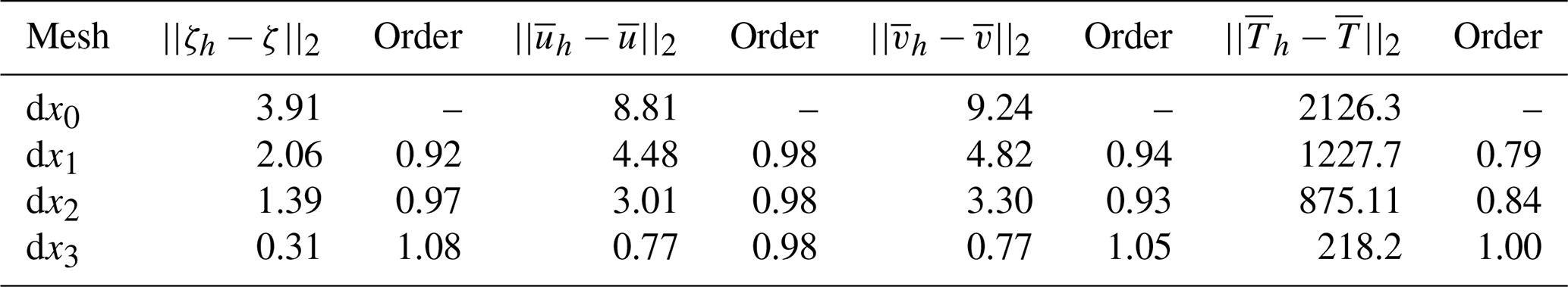
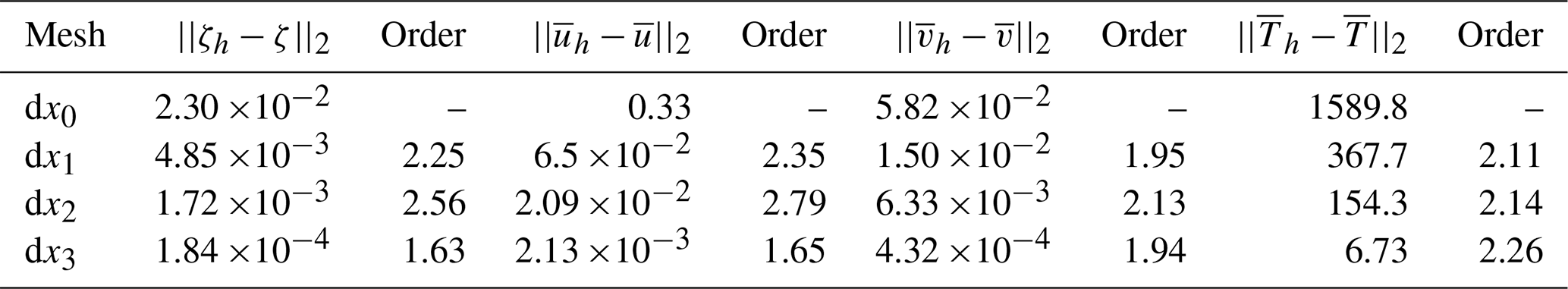
Verification of the DG solution of the mass and momentum equations in the depth-averaged and full three-dimensional case is well documented and can be found in Conroy and Kubatko (2016), Dawson and Aizinger (2005), and Kubatko et al. (2006). To verify our DG solution method for the fully coupled mass, momentum, and energy (depth-averaged) equations, we solve a test problem that is designed to model a free surface wave propagating through a lava channel using the method of manufactured solutions (see Griffiths, 2000, for a discussion on free surface waves in lava channels at high Re number and Le Moigne et al. (2020) for a detailed investigation on standing waves in lava flow channels). We choose $\stackrel{\mathrm{‾}}{u}$, $\stackrel{\mathrm{‾}}{v}$, and H so that the depth-averaged mass equation is satisfied exactly. Specifically, we define

$$\begin{array}{}\text{(49)}& \begin{array}{rl}& \stackrel{\mathrm{‾}}{u}=\widehat{u}\exp \left(-x\right),\\ & \stackrel{\mathrm{‾}}{v}=\widehat{v}\exp (-kx),\\ & H=h+\widehat{\mathit{\zeta }}\exp \left(\text{i}\mathit{\omega }t\right),\end{array}\end{array}$$

with h= constant, $\widehat{u}=$ constant, $\widehat{v}=\widehat{u}ky$, and $\widehat{\mathit{\zeta }}=\exp (-\text{i}\mathit{\omega }\widehat{x})$ where $\widehat{x}=\exp \left(kx\right)/\left(k\widehat{u}\right)$. The dynamical solution consists of a wave propagating in a direction perpendicular to the y axis with wave number $k=\mathrm{5.0}\times {\mathrm{10}}^{-\mathrm{3}}$ m⁻¹ and frequency $\mathit{\omega }=\mathrm{2.0}\times {\mathrm{10}}^{-\mathrm{3}}$ s⁻¹. These values were chosen based on velocity and lava flow thickness data recorded by Patrick et al. (2019) during the pulsing effusion regime associated with Fissure 8 during the 2018 Kīlauea event. We then set

$$\begin{array}{}\text{(50)}& \stackrel{\mathrm{‾}}{T}=\widehat{T}\exp (-k_{T}x),\end{array}$$

with $\widehat{T}=(y^{\mathrm{2}}+T_{\text{wall}})$ and substitute Eqs. (49) and (50) into the mathematical model (Eqs. 13–16) and evaluate the derivative terms using MATLAB's symbolic package. The remainder terms associated with the x momentum equation and the energy equation are then set as artificial source terms that force the numerical solution to be Eqs. (49) and (50). The numerical domain consists of a rectangular channel defined by the Cartesian coordinates x₀=0.0 m, x_L=200.0 m, y₀=0.0 m, y_L=30.0 m. We assume symmetry about the centerline (at y=15 m) and only solve the equations over the half-width of the channel. It can be noted that even though the solutions are guaranteed to remain smooth for all time t (because of the forcing functions), the numerical solution is by no means trivial due to the coupling of the equations through the viscosity. We use four different triangular meshes for the verification of the model. The element size of each mesh is 7.50 m (the so-called dx₀ mesh), 3.75 m (dx₁), 2.50 m (dx₂), and 0.625 m (dx₃), respectively. Results are displayed in Tables 1–3, where it can be noted that the method converges to the analytic solution at a rate of approximately $\mathrm{\ell }+\mathrm{1}/\mathrm{2}$. Further, using 𝒫₂ polynomials on the coarsest mesh gives lower errors than 𝒫₀ polynomials on the finest mesh. It can be noted that for a given computational mesh, a higher-order polynomial approximation will result in a greater computational expense. However, the goal of using high-order polynomial approximations is to use coarser meshes, which results in better computational efficiency in terms of the number of degrees of freedom necessary to achieve a certain level of accuracy (high-order local polynomials produce more accurate results more efficiently than low-order methods). This is explicitly shown in the works of Kubatko et al. (2006), Kubatko et al. (2009), and Conroy et al. (2018).

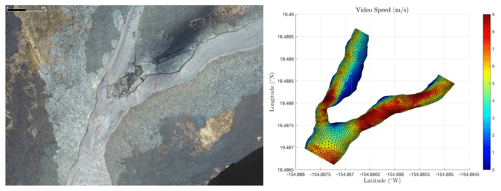
Figure 4 (Left) Zoomed in view of the section of the braided channel system established by Fissure 8 modeled in this work, near UAS site 8 (See Fig. 1). UAS photo by Ryan Perroy, University of Hawai’i-Hilo. (Right) Map view of the lava surface velocity measured using Optical Flow from videos captured by UAS on 22 June 2018. Colors represent magnitude in m/s. Also shown is the finite-element mesh used to evaluate the model.

5 Evaluation: recent eruption of Kīlauea volcano

We evaluate our model using data captured during the 2018 eruption of Kīlauea volcano, Hawai'i. The East Rift Zone of Kīlauea has erupted repeatedly in historical times and continuously since 1983 (Heliker and Mattox, 2003; Wolfe, 1988). A new eruption of unusually large magnitude began on 3 May 2018 in the lower part of the East Rift Zone, with fissures opening in the middle of a residential area (Neal et al., 2019). More than 20 fissures opened during the first 12 d of the eruption, erupting slow-moving, unusually high-viscosity lava at low effusion rates. The behavior changed on 18 May, when much hotter and less viscous lava reached the surface. Advance rates and flow lengths increased, widely impacting property and infrastructure. Complete evacuation orders followed within days. Starting on 28 May, activity focused at Fissure 8, located in the heart of the Leilani Estate subdivision. Fissure 8 remained the source of lava for the remainder of the eruption until its abrupt stop on 4 August. The lava that erupted from Fissure 8 soon established a channel that flowed north and east of the vent, forming a moderately branched channel network 4 km from the vent. The flow field exhibited transitions between flow types: a clear transition from pahoehoe to `a`a surface texture occurred downslope and is apparent on the thermal map (see Fig. 1). Overall, the Fissure 8 lava covered an area of 25 km² and supplied at least 1 ³ of lava (out of at least 1.2 total) over 70 d.

5.1 Observational data

During the 2018 Kīlauea eruption, unoccupied aerial systems (UASs) captured a comprehensive time series of overhead videos of channelized lava (the Fissure 8 flow). The videography campaign was purposefully designed to collect data for “remote rheometry” by hovering above specific sites spaced 200–1300 m apart along the length of the open channel and revisiting them throughout the duration of the eruption.

The proximal (near-vent) sites record pahoehoe lava with little crust cover, while the distal sites capture behavior entirely in the `a`a flow regime. Sites within the braided section of the flow recorded video over parallel channels. Over 500 hover videos at the channel sites were acquired over the course of the Fissure 8 eruption between 30 May and 5 August. In this paper, we focus on videos collected at UAS site 8, capturing a junction point where the main channel split into two branches; see Fig. 4.

5.1.1 Velocity field measurements

We analyze the UAS hover videos using the optical flow technique (Horn and Schunck, 1981; Sun et al., 2010) Optical flow is a well-known computer vision technique used to measure velocities of imaged objects based on the motion of brightness within an image sequence or between frames of a video. Lev et al. (2012) used Optical flow to measure the two-dimensional surface velocities of laboratory-scale basaltic lava flows. We follow the same technique as in Lev et al. (2012), tuning parameters to the specifics of the Kīlauea 2018 UAS footage; see Fig. 4. Length scales for video analysis and channel geometry data are provided from camera lens information and the recorded UAS flight altitude and refined using co-registered digital elevation and orthomosaic images produced from additional UAS data collected at the same or very close time.

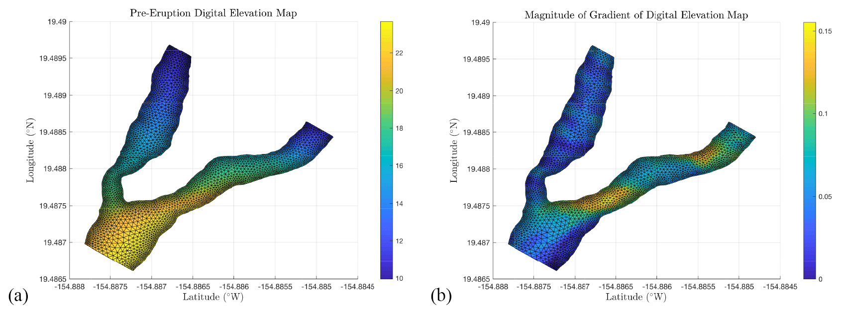
Figure 5 Finite-element partition of the modeled section of the braided channel system. Colors corresponds to (a) topography elevation in meters and (b) the magnitude of the gradient of the topography.

Figure 6 Map view of modeled speed using a value of (a) n=1 and (b) n=2 in the viscosity model. Colors represent velocity magnitude in meters per second.

5.2 Model input

We provide our model with a channel geometry, assumed material properties, inlet velocity, and observed temperature. We use topography data from a pre-eruption digital elevation maps (data from the USGS National Elevation Dataset, with a spatial resolution of 10 m/pixel, USGS, 2002) to calculate the gradient of topography (see Fig. 5). We set the inlet velocity equal to values measured from the UAS video analyzed by optical flow (Fig. 4). Channel edge geometry is obtained from the velocity field (|u|>=0) combined with visible identification of channel boundaries in the UAS image. Figure 5 shows the meshed model domain, with colors depicting the elevation and ground slope used to set up the model.

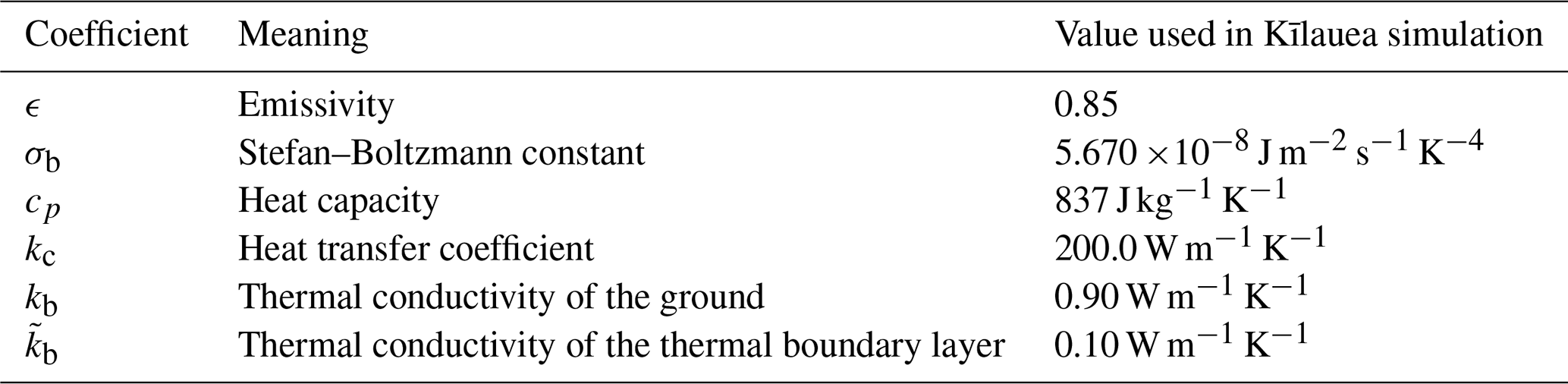
We set the lava density to ρ=1350 kg m⁻³, which, with a nominal gas-free density of Hawaiian basalts of 2700 kg m⁻³ translates to 50 % vesicularity. We set the channel inlet temperature to $\stackrel{\mathrm{‾}}{T}=\mathrm{1152}$ ^∘C and wall and basal temperatures to T_wall=1010 ^∘C and T_ground=477 ^∘C, respectively. The rheological constants in Eq. (19) are set to $A=-\mathrm{4.550}$, B=5805.30, and C=607.80. These values were calculated using the calculator by Giordano et al. (2008) and are specific for the composition of the basalt that erupted during June 2018 from Fissure 8 as measured by XRF analysis (Gansecki et al., 2019). See Table 4 for the coefficient values used in the heat transfer module. It can be noted that because the lava temperature never falls below 950 ^∘C in the Kīlauea simulations, surface heat loss is solely due to radiation.

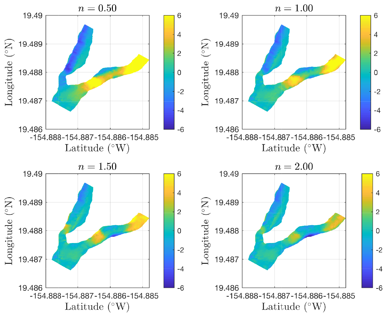
Figure 7 Map view of the difference between modeled lava speed and surface speed obtained from UAS video capture for various power law exponents. Colors represent difference in meters per second.

Table 4 Value of thermal coefficients.

5.3 Model results

All model simulations were executed on a Macbook Pro using Intel's Fortran compiler and on average took 56 min to execute using a time step dt=0.05 s. The finite-element partition of the braided channel system (shown in Fig. 5) consists of 6908 elements with a maximum element size of 8 m and a minimum element size of 1 m. The model's initial conditions were set to the solution of a linearized form of Eqs. (13)–(16) with ζ=0 and h=10 m. Inlet conditions are steady in time, and we set τ_yield=0 in the Herschel–Bulkley model and time step the nonlinear system of Eqs. (13)–(16) to steady state.

Figure 6 shows the lava velocities calculated for the entire domain by our model using exponent values in the viscosity model (Eq. 18) of n=1 (Newtonian) and n=2 (shear-thickening). Key features of the observed flow field, such as the increase in speed after the constriction in the northern branch and the stagnation at the channel split point, are present in both figures. The overall magnitude of the velocity – up to 9 m s⁻¹ – is also in agreement with the observations.

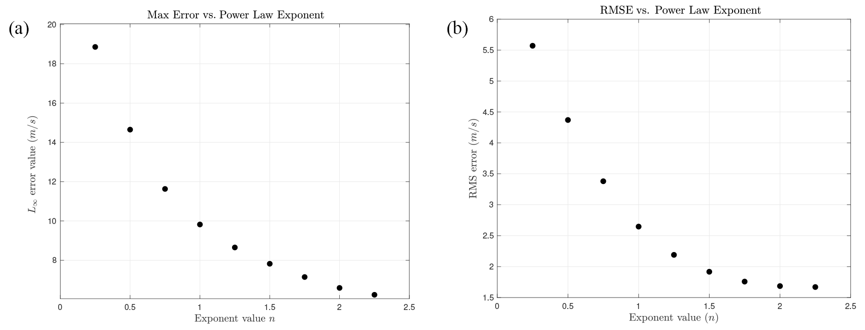
Figure 8 (a) Maximum error in model speed versus power law exponent. (b) Root-mean-square error in model speed versus power law exponent.

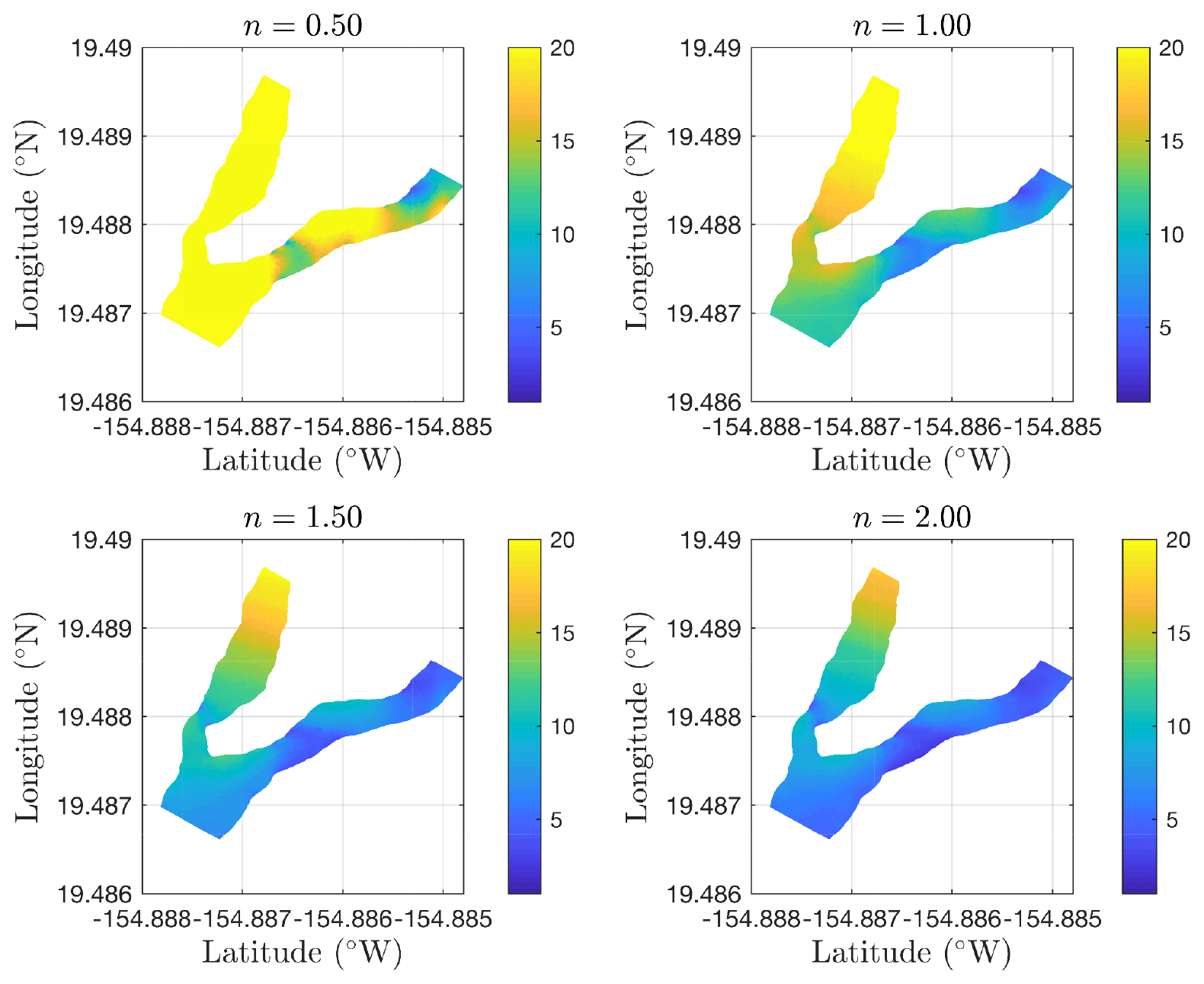
Figure 9 Map view of the modeled lava thickness for various power law exponents. Colors represent lava thickness in meters. Notice that the lava becomes thinner as the value of n increases.

5.4 Discussion

We evaluate the quality of the fit between the model and the observations by comparing the modeled speed with the observed speed for different power law exponent (n) values shown in Fig. 7. Two areas of relatively large error are clear in the southern branch. We attribute these mostly to uncertainties in the underlying topography data. We use a coarse pre-eruption digital elevation map (DEM) for an area where the overall slopes are very gradual (2–3^∘). The mesh and model resolution is very high compared to the coarseness of the DEM (only 10 DEM grid points across the model), which can lead to inaccuracies in slope estimates. In addition, the DEM is from before the eruption, while the velocity data were captured a few weeks after the channel was established. It is possible that by that time some lava had already deposited on the bottom of the channel and modified the topography.

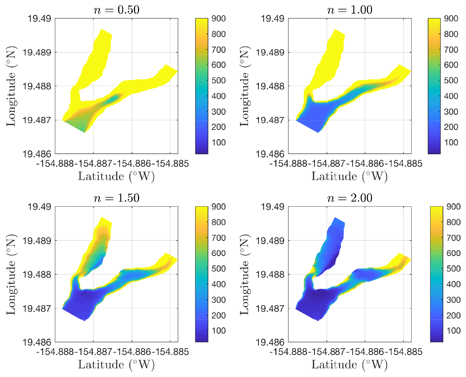
Figure 10 Map view of the effective modeled lava viscosity for various power law exponents. Colors represent viscosity (in Pascal seconds).

An additional source of misfit could be due to the bottom stress calculation. We calculate the thickness of the virtual layer over which the velocity transitions from the depth-integrated velocity to a value of zero (at the bottom boundary) via a two-layer model of vorticity. The two layers correspond to a mixed upper layer and a non-mixed bottom layer where the lava is losing heat due to conduction. While this approach seems to be valid in terms or reproducing lava flow thicknesses observed by USGS surveys (USGS Hawaii Volcano Observatory, 2019), which place lava thicknesses between 5 and 15 m, (alternative methods produce flows that are 3 times too thick), the two-layer model is still a simplification of reality that most likely introduces some errors.

Further, because we are limited to surface speed observations our error metrics will unavoidably have a misfit in them due to the fact that modeled speeds are depth-averaged. This effect will be small in regions of the channel where the Reynolds number is high because the lava speed will be more uniform over its thickness. However, in areas where the Reynolds number is low(er), model speeds will be lower than observations. This is because the section of channel we modeled has minimal crust cover, and therefore there is zero stress at the top boundary of the lava flow, meaning that lava speed should reach a maximum at the surface. This effect is evident in the northern portion of the northern channel and the portion of the southern channel between −154.886 and −154.8855^∘ W.

An interesting aspect of the model worth drawing attention to is how a change in the value of n in the viscosity model affects numerical results. Figures 7 and 8 reveal that the overall fit improves with increasing n values, which corresponds to shear-thickening in our model. Similarly, the thicknesses predicted by our model for larger power law exponent values (Fig. 9) are closer to the range of thicknesses (5–15 m) measured by USGS survey (USGS Hawaii Volcano Observatory, 2019), and the apparent viscosity calculated by our model (shown in Fig. 10) for large n values is similar to rough estimates by the USGS (Weston Thelen, personal communication, 2018).

The lower error measures produced by our model for shear-thickening behavior is a departure from other studies that find lava to behave as a shear-thinning fluid (e.g., Castruccio et al., 2010; Costa et al., 2009; Pinkerton, 1995). The disparity can most likely be attributed to differences in the particle content of the lava; in the studies of Castruccio et al. (2010), Costa et al. (2009), and Pinkerton (1995), the crystal and bubble content of the lava studied was low (< 20 %), whereas samples taken from the Fissure 8 flow during and after the eruption show a wide range of crystallinity and vesicularity, often with very high vesicle fraction of over 50 % (Halverson et al., 2020). The improved overall fit of our model for higher n values is most likely due to this high vesicle fraction and is consistent with the lab experiments of Smith (1997) and Lev et al. (2020) that show high bubble content can produce shear-thickening behavior. In fact, in the experiments of Sayag and Worster (2013), shear-thickening behavior for a constant volume of fluid (as in our investigation) produce flow thicknesses that are less than the shear-thinning case, which is visible in our results in Fig. 9. We conjecture that the increase in the viscosity is due to the fact that as the strain rate increases, the bubbles re-arrange in a fashion that makes it harder for the lava to flow. This effect should be especially pronounced in areas where the strain rate is high (think of the stress associated with solid boundaries in turbulence and how the vorticity created at these boundaries could cause bubbles to run into each other, impeding the flow). This effect is apparent in Fig. 10 for the case n=2, where the effective viscosity is low except in regions of high strain and high(er) Reynolds number, such as near the constriction in the northern channel, at the channel walls where the slope is high in the southern channel, and at the bend area in the southern channel. In the future we will explore mathematical relationships that allow n to be a function of the bubble and crystal content of the lava and examine the sensitivity of the model to non-Newtonian rheological parameters. We plan to infer the best-fitting values for these parameters for a range of locations and times for the Fissure 8 lava flow.

6 Conclusions

We present a novel numerical model for quantifying high-speed lava flows in complex channels. The mathematical model consists of depth-averaged equations of mass, momentum, and energy, and the equations are closed via a nonlinear viscosity model. Because we use discontinuous Galerkin methods to discretize the mathematical model, we are able to capture non-smooth transitions that can occur in lava flows, e.g., jumps in temperature, shear, and viscosity; see Fig. 10. We overcome a major limitation to many depth-integrated models in terms of the need to use an adjustable friction coefficient by solving a heat transfer boundary layer problem coupled with a calculation for the thickness of a virtual layer over which the velocity transitions from the depth-integrated velocity to a value of zero (at the bottom boundary) via a two-layer model of vorticity. This novel approach results in lava flow thicknesses that are in the range of observed values as compared to simple linear schemes that produce flow thicknesses that are 3 times too thick. Further, the use of unstructured triangular meshes allows the model to accurately resolve complex braided channel systems that are commonly produced by basaltic lava flows. This was demonstrated on a section of the complex braided channel system that was created by the Fissure 8 flow from the 2018 Kīlauea lower East Rift Zone eruption, with model results matching observational results quantitatively well. Future work will include using the new versatile model as a tool to infer lava properties and flux during volcanic crises.

Appendix A: List of symbols

Symbol	Name	Definition
A	consistency constant	see Sect. 2.1
Aw	wetted area	Aw=wH
αrs	Runge–Kutta coefficient	see Sect. 3.3
B	consistency constant	see Sect. 2.1
b	discrete DG spatial matrix	see Sect. 3.3
βrs	Runge–Kutta coefficient	see Sect. 3.3
C	consistency constant	see Sect. 2.1
dA	differential area	–
$\text{d}{x}_{\mathrm{0}},\mathrm{\dots },\text{d}{x}_{\mathrm{3}}$	mesh size in verification test case	–
Δt	numerical time step	–
δsΔt	sub-time-step in Runge–Kutta method	see Sect. 3.3
δz	length of virtual bottom boundary layer	${\mathit{\delta }}_z=({\mathit{\delta }}_{zx},{\mathit{\delta }}_{zy}{)}^{\prime }$
ϵ	emissivity of lava	see Table 4
F	flux function matrix	see Eq. (35)
$\widehat{F}$	numerical flux function	see Eq. (41)
fb	body force vector	${\mathit{f}}_{\text{b}}={\left(g_x,g_y,g_z\right)}^{\prime }$
fx	x comp. of depth-integrated horizontal shear stress	$f_x={\int }_{-h}^{\mathit{\zeta }}\frac{\partial {\mathit{\tau }}_{xx}}{\partial x}+\frac{\partial {\mathit{\tau }}_{yx}}{\partial y}\text{d}z$
fy	y comp. of depth-integrated horizontal shear stress	$f_y={\int }_{-h}^{\mathit{\zeta }}\frac{\partial {\mathit{\tau }}_{xy}}{\partial x}+\frac{\partial {\mathit{\tau }}_{yy}}{\partial y}\text{d}z$
gx, gy, gz	x, y, z components of gravitational acceleration	–
H	total depth of flow	$H=\mathit{\zeta }+h$
ℋ	Hilbert space	infinite dimensional space with finite energy
h	steady reference depth of flow	see Sect. 2.3
hb	depth of bottom thermal boundary layer	see Sect. 2.2
hw	thickness of thermal boundary layer	–
I	identity matrix	$\left[\begin{array}{cccc}\mathrm{1}& \mathrm{0}& \mathrm{0}& \mathrm{0}\\ \mathrm{0}& \mathrm{1}& \mathrm{0}& \mathrm{0}\\ \mathrm{0}& \mathrm{0}& \mathrm{1}& \mathrm{0}\\ \mathrm{0}& \mathrm{0}& \mathrm{0}& \mathrm{1}\end{array}\right]$
i	index counter for equations in Eqs. (13)–(16)	$i=\mathrm{1},\mathrm{\dots },\mathrm{4}$
$\widehat{i}$	unit vector in x coordinate direction	–
i	imaginary number	$i=\sqrt{-\mathrm{1}}$
J	Jacobian matrix	see Sect. 3.2.1
Jx	Jacobian matrix in x direction	see Sect. 3.2.1
Jy	Jacobian matrix in y direction	see Sect. 3.2.1
j	index counter for the set of elements in 𝒯h	$j=\mathrm{1},\mathrm{\dots },\mathcal{N}$
$\widehat{j}$	unit vector in y coordinate direction	–
𝒦	lava consistency	Pa s
𝒦0	lava consistency constant	sn−1
k	free surface wave number	m−1
$\widehat{k}$	unit vector in z coordinate direction	–
kb	thermal conductivity of ground	see Table 4
${\stackrel{\mathrm{̃}}{k}}_{\text{b}}$	thermal conductivity of bottom boundary layer	see Table 4
kc	convection constant	see Table 4
kT	heat transfer coefficient
L2	L2 error norm	$\left|\right|\cdot |{|}_{\mathrm{2}}={\left({\int }_{{\mathrm{\Omega }}_j}{\left(\mathit{U}-{\mathit{U}}_h\right)}^{\mathrm{2}}\text{d}A\right)}^{\mathrm{1}/\mathrm{2}}$
ℒhp	right hand side of ODE	see Sect. 3.3
Λ( )	diagonal matrix of eigenvalues	see Sect. 3.2.1
λ	an eigenvalue of J	see Sect. 3.2.1
λmax	maximum eigenvalue of J	see Sect. 3.2.1

Symbol	Name	Definition
l	degree of freedom index for polynomial basis	see Sect. 3
ℓ	degree of polynomial basis	see Sect. 3
$\stackrel{\mathrm{̃}}{\mathbf{M}}$	finite-element mass matrix	see Sect. 3.3
m	number of eigenvalues of J	see Sect. 3.2.1
μ	viscosity	Pa s
𝒩	number of elements in 𝒯h	–
n	viscosity power law exponent	see Sect. 2.1
$\widehat{\mathit{n}}$	normal vector	vector perpendicular to a plane
Ωj	element j in 𝒯h	–
ω	vorticity	see Eq. (23)
ω	free surface wave frequency	s−1
P	pressure flux	$P=\frac{\mathrm{1}}{\mathrm{2}}{g}_z\left(H^{\mathrm{2}}-h^{\mathrm{2}}\right)$
𝒫	polynomial space for basis functions	see Sect. 3
Pw	wetted perimeter	$P_w=w+\mathrm{2}H$
p	pressure	Pa
∂Ω	channel domain boundary	–
∂Ωj	boundary of element j in 𝒯h	–
Πh	slope limiter	see Cockburn and Shu (2001)
ϕ	basis functions	combinations of Jacobi polynomials
ψ	test function	ψ∈𝒱
ψh	finite-element approximation of ψ	see Eq. (39)
ψl	polynomial coefficients of ψh	see Eq. (39)
Qin	channel inflow flux	m3 s−1
q	heat flux	$\mathit{q}={\left(k_T\frac{\partial T}{\partial x},k_T\frac{\partial T}{\partial y},k_T\frac{\partial T}{\partial z}\right)}^{\prime }$
$\dot{\mathit{q}}$	internal heat generation and dissipation	–
$\dot{\stackrel{\mathrm{‾}}{q}}$	internal heat generation and dissipation	–
qb	bottom heat flux	see Sect. 2.2
${\stackrel{\mathrm{‾}}{q}}_i$	depth-integrated internal heat flux	–
qs	surface heat flux	see Sect. 2.2
R	vector of DG spatial operator	see Sect. 3.3
ℛ( )	matrix of right eigenvectors of J	see Sect. 3.2.1
${\mathcal{R}}_{\left(\right)}^{-\mathrm{1}}$	matrix of left eigenvectors of J	see Sect. 3.2.1
Re	Reynold's number	$\mathit{Re}=\frac{\mathit{\rho }\left|\right|\mathit{u}\left|\right|A_{\text{w}}}{\mathit{\mu }{P}_w}$
r	eigenvector of J	see Sect.  3.2.1
ρ	density	kg m−3
r, s	index counters in Runge–Kutta time-stepper	–
S	source vector	see Eq. (35)
𝒮	number of Runge–Kutta stages	–
sgn()	sign of argument	–
σb	Stefan–Boltzmann constant	see Table 4
σwall	normal stress vector at wall	$(-\widehat{\mathit{n}}\mathit{\tau }{)}^{\prime }$
T	temperature	K
$\stackrel{\mathrm{‾}}{T}$	depth-averaged temperature	$\stackrel{\mathrm{‾}}{T}=\frac{\mathrm{1}}{H}{\int }_{-h}^{\mathit{\zeta }}T\text{d}z$
$\widehat{T}$	amplitude of $\stackrel{\mathrm{‾}}{T}$ in verification test	see Sect. 4
𝒯h	finite-element triangulation of Ω	${\mathcal{T}}_h={\left\{{\mathrm{\Omega }}_j\right\}}_{j=\mathrm{1}}^{\mathcal{N}}$
Tatm	atmospheric temperature	K
Tground	ground temperature	K
t	time	s
$\widehat{\mathit{t}}$	tangential vector	vector parallel to a plane
ti	initial time in averaging window	s
tf	final time in averaging window	s

Symbol	Name	Definition
τ	stress tensor	see Sect. 2
τb	bottom stress vector	${\mathit{\tau }}_{\text{b}}={\left({\mathit{\tau }}_{{\text{b}}_x},{\mathit{\tau }}_{{\text{b}}_y}\right)}^{\prime }$
τs	surface stress vector	${\mathit{\tau }}_{\text{s}}={\left({\mathit{\tau }}_{{\text{s}}_x},{\mathit{\tau }}_{{\text{s}}_y}\right)}^{\prime }$
σwall	normal stress vector at wall	$(-\widehat{\mathit{n}}\mathit{\tau }{)}^{\prime }$
(  )′	transpose operator	$(u,v,w{)}^{\prime }=\left[\begin{array}{c}u\\ v\\ w\end{array}\right]$
U	solution vector	see Eq. (35)
$\stackrel{\mathrm{̃}}{\mathit{U}}$	vector of polynomial coefficients (degrees of freedom)	see Sect. 3.3
Uh	finite-element approximation of U	see Eq. (38)
Ul	polynomial coefficients of Uh	see Eq. (38)
u	depth dependent velocity	$\mathit{u}=(u,v,w{)}^{\prime }$
$\left|\right|\mathit{u}\left|\right|$	magnitude of velocity	$\left|\right|\mathit{u}\left|\right|=(u^{\mathrm{2}}+v^{\mathrm{2}}+w^{\mathrm{2}}{)}^{\mathrm{1}/\mathrm{2}}$
$\stackrel{\mathrm{‾}}{\mathit{u}}$	depth-averaged velocity vector	$\stackrel{\mathrm{‾}}{\mathit{u}}={\left(\frac{\mathrm{1}}{H}{\int }_{-h}^{\mathit{\zeta }}u\text{d}z,\frac{\mathrm{1}}{H}{\int }_{-h}^{\mathit{\zeta }}v\text{d}z\right)}^{\prime }$
u	x component of velocity	$u=\text{d}x/\text{d}t$
$\widehat{u}$	amplitude of $\stackrel{\mathrm{‾}}{u}$ in verification test	see Sect. 4
𝒱	admissible space of functions	𝒱∈ℋ
𝒱hp	finite dimensional subspace	𝒱h∈𝒱
v	y component of velocity	$v=\text{d}y/\text{d}t$
$\widehat{v}$	amplitude of $\stackrel{\mathrm{‾}}{v}$ in verification test	see Sect. 4
w	z component of velocity	$w=\text{d}z/\text{d}t$
$\stackrel{\mathrm{‾}}{w}$	measure of depth-averaged vertical velocity	see Eq. (24)
$\stackrel{\mathrm{̃}}{\mathbf{w}}$	right-hand-side function in RK method	see Sect. 3.3
win	channel width at inlet	–
x	Cartesian coordinate	$\mathbf{x}=(x,y,z{)}^{\prime }$
x0, xL	x coordinate of inlet and outlet boundaries	–
y0, yL	y coordinate of channel walls	–
$\stackrel{\mathrm{̃}}{z}$	thermal boundary layer coordinate	$\stackrel{\mathrm{̃}}{z}\in \left[\mathrm{0},-h_{\text{b}}\right]$
zb	z coordinate where thermal boundary layer begins	see Sect. 2.2
ζ	free surface elevation	$\mathit{\zeta }=H-h$
$\widehat{\mathit{\zeta }}$	amplitude of surface elevation in verification test	see Sect. 4
τyield	yield strength of lava	–
∇	gradient operator	$\mathrm{\nabla }={\left(\frac{\partial }{\partial x},\frac{\partial }{\partial y},\frac{\partial }{\partial z}\right)}^{\prime }$
$\stackrel{\mathrm{‾}}{\mathrm{\nabla }}$	horizontal gradient operator	$\stackrel{\mathrm{‾}}{\mathrm{\nabla }}={\left(\frac{\partial }{\partial x},\frac{\partial }{\partial y}\right)}^{\prime }$
0	vector of zeros	${\left(\mathrm{0},\mathrm{\dots },\mathrm{0}\right)}^{\prime }$